Phonon influence on the measurement of spin states in double quantum dots using the quantum point contact

Abstract

We study the influence of phonon scattering on the noise characteristics of a quantum point contact coupled to a two-electron system in a double quantum dot, as proposed for a singlet-triplet measurement scheme in a double-dot system. We point out that at low temperatures phonon-induced relaxation to the ground state suppresses transitions to doubly occupied singlet states which are the source of detectable current fluctuations in this measurement scheme. Thus, for a relatively strong electron-phonon interaction present in the system, the two configurations display the same noise characteristics. In this way, coupling to phonons reduces the distinguishability between the singlet and triplet configurations. Under such conditions, the proposed measurement scheme is no longer valid even though the times of the measurement-induced decoherence of an initial singlet-triplet superposition and of the localization into the singlet or triplet subspace remain essentially unchanged.

I Introduction

One of the most promising proposals for solid-state qubit implementation is based on the utilization of the spin states of electrons confined in quantum dots (QDs). The original idea of coding the qubit in the two states of a single electron spinloss98 still inspires a lot of interest, since relatively long spin coherence times have been reported, and the experimental techniques for the preparation, manipulation, and readout of such qubits are being rapidly developednowack07 ; greilich09 ; kim11 . The study of two electron spin states in double QDs (DQDs) is a natural extension of the problem, which serves to examine two-qubit coherence and inter-qubit interactionscoish05 ; johnson05 ; pfund07 ; stepanenko12 ; maune12 . Furthermore, to facilitate electrical control of electron-spin qubits, two-spin encoding has been proposedlevy02 ; petta05 ; taylor07 , which involves spin-singlet and spin-triplet configurations serving as the $|0\rangle$ and $|1\rangle$ qubit states. This approach proves to be promising as well, as is seen, e.g., in the recent demonstration of entanglement between two singlet-triplet qubitsshulman12 .

The quantum point contactbeenakker91 (QPC) measurement of charge states in a lateral DQD defined by gate potentials in a two dimensional electron gas involves monitoring the current flowing through the QPC which depends on the occupation of the QDs due to a Coulomb interaction between the electrons confined in the QD and electrons traveling through the QPCbarrett06 ; stace04 . This measurement scenario is a realization of the so called weak measurementnielsen00 , where the measured system is only weakly coupled to the measuring device. Contrary to the projective measurement, this measurement is not instantaneous, as both the localization of the QD states into the measurement basis and acquiring the data needed to distinguish between the basis states take time. Apart from the measurement time, another relevant factor is the attainable distinguishability of states, since even after an infinitely long measurement time it may not be possible to completely distinguish between the measurement basis states. On the other hand, a weak measurement is typically less destructive to the measured system than an instantaneous projective measurement. Furthermore, such a measurement is the only option in many involved quantum systems which are hard to access experimentally. Hence, the QD-QPC measurement setup is commonly used experimentally to study QD occupations at very low temperaturesaverin05a ; meunier06 ; rogge05 ; barthel09 ; cassidy07 ; bylander05 ; elzerman04 . As we have previously shown, phonon effects do not interfere with the charge measurement in any significant waymarcinowski11 , since while they strongly affect the coherence times of QD states, phonons do not affect the localization times or the distinguishability between the measurement basis states in this setup.

The measurement of spin states of electrons confined in QDs is much more complicated and typically involves spin-to-charge conversion prior to a QPC measurement of the chargemeunier06 ; cassidy07 ; elzerman04 ; petta05 . An alternative scheme for the direct measurement of the spin symmetry (singlet–triplet) of two-electron states confined in a DQD was proposed in Ref. [barrett06, ]. Here, the quality of the measurement relies on QPC current noise being different for the singlet and triplet spin symmetries. The disparity of current fluctuations is due to the fact that, according to Pauli exclusion principle, states with both electrons localized in the same QD are allowed in the spin-singlet configuration, but not for spin-triplet case. Hence, the electron charge distribution will fluctuate during the measurement process due to the QD-QPC interaction only if the electrons are in the spin-singlet state, leading to enhanced QPC current noise for this spin configuration.

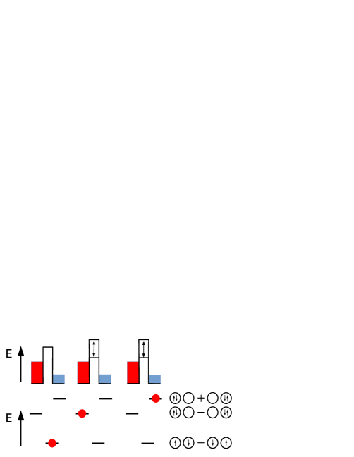
Figure 1: Schematic representation of the changes of the QPC barrier height due to Coulomb interaction with different spatial configurations of the three spatially distinct DQD spin singlet states. The top part shows the QPC barrier height corresponding to the occupation of the DQD represented in the bottom part of the figure. The two doubly occupied states are superpositions of configurations with charges adjacent or remote from the QPC which results in fluctuations of the QPC barrier.

In this paper, we study the interplay of phonon-induced effects on two-electron DQD spin states and the QPC measurement of these states in the high bias regime. In this setup, phonon-assisted interdot tunneling processes at low temperatures lead to relaxation of electrons in the spin-singlet configuration to their lowest energy state grodecka08a (with the two electrons located in different dots to minimize the repulsive Coulomb interaction), which should strongly affect the distinguishability between the singlet and triplet states. As we find out, while the additional, phonon-induced decoherence channel obviously increases the rate of dephasing of singlet-triplet superpositions, it affects neither the time needed for the measured state to localize in the singlet or triplet state (“collapse” of the state vector) nor the data acquisition time needed to perform the measurement. We show, however, that phonon-assisted transitions counteract the enhanced QPC current fluctuations in the case of the singlet state by suppressing the occupation fluctuations. Thus, the carrier-phonon interaction leads to a reduced distinguishability of two-electron spin states. When the strength of the phonon-QD interaction is comparable to the strength of the QPC-QD coupling, the measurement process is completely suppressed and an extension of the measurement time cannot yield any improvement on the quality of the measurement.

The paper is organized as follows. In Sec. II, we introduce the system and define the model to be studied. In Sec. III, we derive the quantum master equation in Lindblad form for the dynamics of the DQD-QPC system with the electron-phonon interaction included. In Sec. IV, we introduce the stochastic simulation method in the conditional density matrix formalism, which allows us to perform simulations of single measurement runs. The general results are presented in Sec. V, while the noise characteristics are discussed in Sec. VI. Sec. VII concludes the paper.

II The system and the Hamiltonian

We consider two electrons confined in a gate defined lateral DQD composed of two identical QDs coupled to a QPC, following Ref. [barrett06, ]. The QPC is located near one of the dots (say, right) in such a way that the current flowing through the QPC is only affected by the occupation of this one dot. We assume that the electrons are in the ground state manifold of single electron orbital states and that the excited states are energetically far beyond the double charging energy. Because of this assumption, only six two-electron states are taken into account. The four lower energy states involve electrons confined in separate QDs, one with singlet spin symmetry and three with triplet spin symmetries. Due to the Coulomb repulsion energy, the other two states which are superpositions of doubly occupied QD states and must have singlet spin symmetry due to the Pauli exclusion principle, are energetically separated from the other two-electron states considered. The electrons tunneling through the QPC interact with the electrons in the right QD due to the dependence of the QPC tunneling barrier on the occupation of the right dot (the larger this occupation, the higher the tunneling barrier). When the QD electrons are in one of the lower energy states, the height of the QPC tunneling barrier is robust and the current flowing through the QPC is Poissonian (the noise is characteristic for noninteracting electrons travelling through a time-independent potential barrier). The situation is different when the DQD is in one of the higher singlet states which are superpositions of doubly occupied states, because the height of the tunneling barrier is different when both electrons are in the right dot and when both electrons are in the left dot (see Fig. 1). The resulting fluctuations of the barrier height lead to an enhancement of the QPC current noise. Since the interaction between the DQD and the QPC cannot change the electron spin symmetry, only the low energy singlet state is coupled to higher energy states. Hence, if the DQD is in the triplet state the QPC current noise remains Poissonian throughout the evolution, but if the DQD is in the singlet state, the QPC induces DQD transitions between different singlet states, which leads to different noise characteristics (and much greater current noise). This difference in the magnitude and the statistical characteristics of the QPC current noise allows one to distinguish between the DQD triplet and singlet states, and is the basis of the measurement scheme proposed in Ref. [barrett06, ]. In order for the non-elastic tunneling events at the QPC to provide sufficient energy for inducing a transition to a doubly occupied state, the QPC has to be operated in the high bias regime, that is, the difference between the chemical potentials in the source and drain must be larger than the double charging energy. Apart from this requirement, no fine tuning of the bias voltage is needed, in contrast to the spin-charge conversion protocols reilly07 .

Since QDs are solid state systems, we include the coupling between the confined electrons and vibrations of the surrounding crystal lattice (phonons), especially that the time scales of phonon-related processes in such a system are comparable to the times over which QPC current traces are observedmarcinowski11 ; cassidy07 ; bylander05 . The interaction between the DQD electrons and the phonon environment cannot change the spin symmetry of the DQD state (similarly as the DQD-QPC interaction), hence, it does not couple singlet and triplet states. In fact, as shown later, phonons induce exactly the same transitions as the DQD-QPC interaction and at low temperatures phonon emission from the DQD is expected to suppress the QPC induced singlet-singlet transitions. Since the transitions to higher (singlet) energy states result in the increased QPC current which serves to distinguish between the singlet and triplet DQD configurations, such a suppression leads to a diminished distinguishability between the states and consequently can undermine the usefulness of the measurement scheme.

The Hamiltonian of the system is given by

$$H_{\mathrm{tot}}=H_{{\mathrm{DQD}}}+H_{{\mathrm{leads}}}+H_{{\mathrm{tun}}}+H_{{\mathrm{ph}}}+H_{{\mathrm{e-ph}}}.$$

The first term describes two electrons in the DQD structurebarrett06 ; roszak09

$$H_{{\mathrm{DQD}}}=\Delta\sum_{\sigma=\uparrow,\downarrow}(a_{R\sigma}^{\dagger}a_{L\sigma}+a_{L\sigma}^{\dagger}a_{R\sigma})+U\sum_{i=R,L}n_{i\downarrow}n_{i\uparrow},$$

where $\Delta$ is the amplitude of the tunneling between the dots, $a_{i\sigma}$, $a_{i\sigma}^{\dagger}$ are the annihilation and creation operators of an electron in dot $i=\mathrm{R,L}$ with spin $\sigma=$ $\uparrow,\downarrow$, $n_{i\sigma}=a_{i\sigma}^{\dagger}a_{i\sigma}$ gives the number of electrons with spin $\sigma$ in dot $i$, and $U$ is the Coulomb charging energy for adding a second electron to a QD.

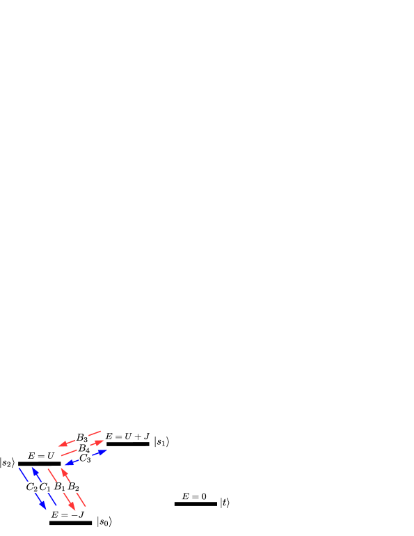
Figure 2: Schematic representation of the energy levels of the system and the allowed transitions between $H_{{\mathrm{DQD}}}$ eigenstates induced by the interaction of electrons in the DQD with the QPC ($C_{i}$ operators, blue arrows) and with the phonon reservoir ($B_{i}$ operators, red arrows).

The eigenstates of $H_{{\mathrm{DQD}}}$ are

$$|t_{0}~{}\!\rangle = \frac{1}{\sqrt{2}}(|\uparrow\downarrow\rangle+|\downarrow\uparrow\rangle),$$ (1a)

$$|t_{+}\rangle = |\uparrow\uparrow\rangle,$$ (1b)

$$|t_{-}\rangle = |\downarrow\downarrow\rangle,$$ (1c)

$$|s_{0}\rangle = \xi^{\prime}\Big{(}|\uparrow\downarrow\rangle-|\downarrow\uparrow\rangle\Big{)}-\xi\Big{(}|d_{L}\rangle+|d_{R}\rangle\Big{)},$$ (1d)

$$|s_{1}\rangle = \xi\Big{(}|\uparrow\downarrow\rangle-|\downarrow\uparrow\rangle\Big{)}+\xi^{\prime}\Big{(}|d_{L}\rangle+|d_{R}\rangle\Big{)},$$ (1e)

$$|s_{2}\rangle = \frac{1}{\sqrt{2}}\Big{(}|d_{L}\rangle-|d_{R}\rangle\Big{)},$$ (1f)

where $|\sigma\sigma^{\prime}\rangle=a^{\dagger}_{L\sigma}a^{\dagger}_{R\sigma^{\prime}}|0\rangle$ denote singly occupied states, and $|d_{i}\rangle=a^{\dagger}_{i\uparrow}a^{\dagger}_{i\downarrow}|0\rangle$, $i=L,R$, are doubly occupied states. The parameters are equal to $\xi=1/\sqrt{2}\sin(\theta/2)$ and $\xi^{\prime}=1/\sqrt{2}\cos(\theta/2)$, where $\theta=\mathrm{atan}(4\Delta/U)$. The triplet states are degenerate in zero magnetic field, and their eigenenergy is chosen as zero. The singlet state eigenenergies are then, respectively, $-J,U,U+J$, where $J=1/2(\sqrt{U^{2}+16\Delta^{2}}-U)$ is the exchange splitting between lowest energy singlet and triplet states (see Fig. 2).

The second term describes the QPC leadsgurvitz96 ; stace04 ; barrett06 ; goan01 ,

$$H_{{\mathrm{leads}}}=\hbar\sum_{p,\sigma}\omega_{Sp}a_{Sp\sigma}^{\dagger}a_{Sp\sigma}+\hbar\sum_{p,\sigma}\omega_{Dp}a^{\dagger}_{Dp\sigma}a_{Dp\sigma},$$ (2)

where $\hbar\omega_{np}$ is the energy of an electron in lead $n=\mathrm{S,D}$ (source, drain) and in mode $p$, $a_{np\sigma}$, $a_{np\sigma}^{\dagger}$ are the corresponding electron annihilation and creation operators with the additional distinction of spin $\sigma$. The third term describes the tunneling of electrons through the QPCstace04 ; barrett06 ; goan01 ,

$$H_{{\mathrm{tun}}}=\sum_{p,q,\sigma}(T_{pq}+\chi_{pq}n_{R})a_{Sp\sigma}^{\dagger}a_{Dq\sigma}+\mbox{H.c.}$$ (3)

It consists of two parts: electron tunneling independent of the DQD is described by the constants $T_{pq}$, while $\chi_{pq}$ quantifies the tunneling dependent on the Coulomb interaction of QPC electrons with electrons in the DQD. This depends on the total number of electrons in the right dot, $n_{\mathrm{R}}=n_{\mathrm{R}\uparrow}+n_{\mathrm{R}\downarrow}$. The tunneling constants are assumed to be slowly varying over the energy range where tunneling is allowedgurvitz96 ; barrett06 , hence we make the assumption $T_{pq}\approx T$ and $\chi_{pq}\approx\chi$. We assume that the QPC operates in the high bias regime, that is, the chemical potential offset between the leads is large enough to induce transitions to doubly excited states barrett06 .

The last two terms in the Hamiltonian describe the energy of the free phonons,

$$H_{{\mathrm{ph}}}=\sum_{\bm{k},\lambda}\hbar\omega_{\bm{k},\lambda}b_{\bm{k},\lambda}^{\dagger}b_{\bm{k},\lambda},$$ (4)

and the interaction between phonons and electrons confined in the DQDkrummheuer02 ; vagov02a ; vagov03 ; grodecka05a ; roszak10 ,

$$H_{{\mathrm{e-ph}}}=\sum_{\sigma,i}\sum_{\bm{k},\lambda}F_{i}^{(\lambda)}(\bm{k})a_{i\sigma}^{\dagger}a_{i\sigma}(b_{\bm{k},\lambda}+b_{-\bm{k},\lambda}^{\dagger}).$$ (5)

In Eqs (4) and (5), $b_{\bm{k},\lambda}$ and $b_{\bm{k},\lambda}^{\dagger}$ are phonon annihilation and creation operators for a phonon from branch $\lambda$ with wave vector $\bm{k}$, $\hbar\omega_{\bm{k},\lambda}$ are the corresponding energies, $F_{\mathrm{L/R}}^{(\lambda)}(\bm{k})=F^{(\lambda)}(\bm{k})e^{\pm ik_{x}D/2}$ are electron-phonon coupling constants, and $D$ is the inter-dot distance. We include deformation potential and piezoelectric couplings. The coupling constants for the longitudinal ($\lambda=l$) and transverse ($\lambda=t_{1,2}$) acoustic phonon branches are mahan00 ; mahan72 ; roszak09 ; roszak05b ,

$$F^{(l)}(\bm{k})=\sqrt{\frac{\hbar}{2\rho_{c}v\omega_{\bm{k},l}}}\left[\sigma k-i\frac{de}{\varepsilon_{0}\varepsilon_{s}}M_{l}(\hat{\bm{k}})\right]\mathcal{F}(\bm{k})$$ (6)

and

$$F^{(t_{1},t_{2})}(\bm{k})=-i\sqrt{\frac{\hbar}{2\rho_{c}v\omega_{k,t}}}\frac{de}{\varepsilon_{0}\varepsilon_{s}}M_{t_{1},t_{2}}(\hat{\bm{k}})\mathcal{F}(\bm{k}),$$ (7)

respectively, where $e$ denotes the electron charge, $\rho_{c}$ is the crystal density, $v$ is the normalization volume for the phonon modes, $d$ is the piezoelectric constant, $\varepsilon_{0}$ is the vacuum permittivity, $\varepsilon_{s}$ is the static relative dielectric constant, and $\sigma$ is the deformation potential constant. The functions $M_{\lambda}$ depend on the orientation of the phonon wave vector. For the zinc-blende structure they are given bymahan72

$$M_{\lambda}(\hat{\bm{k}})=2[\hat{k}_{x}\hat{k}_{y}(\hat{e}_{\lambda,\bm{k}})_{z}+\hat{k}_{y}\hat{k}_{z}(\hat{e}_{\lambda,\bm{k}})_{x}+\hat{k}_{z}\hat{k}_{x}(\hat{e}_{\lambda,\bm{k}})_{y}],$$

where $\hat{\bm{k}}=\bm{k}/k$ and $\hat{e}_{\lambda,\bm{k}}$ are unit polarization vectors. The form factors $\mathcal{F}(\bm{k})$ depend on wave-function geometry and are given by

$$\mathcal{F}(\bm{k})=\int\mathrm{d}^{3}\bm{r}\psi^{*}(\bm{r})e^{i\bm{k}\cdot\bm{r}}\psi(\bm{r}),$$

where $\psi(\bm{r})$ is the envelope wave function of an electron centered at $\bm{r}=0$.

III Lindblad Master equation

To describe DQD dynamics averaged over a large number of repetitions of the measurement procedure it is convenient to use the quantum master equation (QME) approach in Lindblad form (Markov approximation). The problem is relatively involved due to the interaction of our system of interest (the DQD) with two reservoirs, a bosonic and a fermionic one. Since we assume that these reservoirs are uncorrelated with each other, they can be treated separately, yielding unconvoluted terms in the QMEbreuer02 ,

$$\dot{\rho}(t) = -\frac{i}{\hbar}[H_{{\mathrm{DQD}}},\rho]$$

$$+\frac{1}{\hbar^{2}}\left(\sum_{i}^{3}C_{i}\rho C_{i}^{\dagger}-\sum_{i}^{3}\frac{1}{2}(C_{i}^{\dagger}C_{i}\rho+\rho C_{i}^{\dagger}C_{i})\right)$$

$$+\frac{1}{\hbar^{2}}\left(\sum_{i}^{4}B_{i}\rho B_{i}^{\dagger}-\sum_{i}^{4}\frac{1}{2}(B_{i}^{\dagger}B_{i}\rho+\rho B_{i}^{\dagger}B_{i})\right).$$

Here, the first term on the right side of the equation describes the free DQD evolution, while the Lindblad operators $C_{i}$ relate to the DQD-QPC interaction, and $B_{i}$ describe phonon-related effects.

The Lindblad operators $C_{i}$ may be obtained following Ref. [barrett06, ] in the Born-Markov and rotating wave approximations (RWA) and assuming independence of the tunneling rates on the initial and final electron state within the relevant energy regime. The operators are of the formbarrett06

$$C_{1} = \nu\sqrt{\frac{V-(U+J)}{\hbar}}\sin\frac{\theta}{2}|s_{2}\rangle\!\langle s_{0}|,$$

$$C_{2} = \nu\sqrt{\frac{V+(U+J)}{\hbar}}\sin\frac{\theta}{2}|s_{0}\rangle\!\langle s_{2}|,$$

$$C_{3} = \sqrt{\frac{V}{\hbar}}\left[(\mathcal{T}+\nu)\mathbb{I}+\nu\cos\frac{\theta}{2}\left(|s_{1}\rangle\!\langle s_{2}|+|s_{2}\rangle\!\langle s_{1}|\right)\right],$$

where $V=(\mu_{S}-\mu_{D})$ is the QPC bias, $\mathcal{T}=\sqrt{4\pi g_{L}g_{R}}T$ is the unconditional tunneling constant related to $T_{pq}$ of Eq. (3) and $\nu=\sqrt{4\pi g_{L}g_{R}}$ is a constant stemming from tunneling conditioned on the occupation of the right QD (related to $\chi_{pq}$), where $g_{i}$ is the density of states of the $i$-th lead ($i=L,R$). $C_{1}$ and $C_{2}$ describe inelastic transitions which involve energy transfer between the DQD and QPC electrons accompanied by transitions between the low energy state $|s_{0}\rangle$ and high energy states (blue arrows in Fig 2). The quasi-elastic transition between states of similar energy $|s_{1}\rangle$ and $|s_{2}\rangle$ is represented by the Lindblad operator $C_{3}$; this operator also describes the fully elastic processes corresponding to electrons tunneling through the QPC without disturbing the DQD state (which are also possible in a spin-triplet DQD state).

To describe the electron-phonon interaction it is convenient to rewrite the appropriate Hamiltonian (Eq. (5)) in the basis of DQD eigenstatesroszak09 , Eqs. (1),

$$H_{\mathrm{e-ph}} = \sqrt{2}\left[\xi^{\prime}(|s_{1}\rangle\!\langle s_{2}|+|s_{2}\rangle\!\langle s_{1}|)\right.$$

$$\left.-\xi(|s_{0}\rangle\!\langle s_{2}|+|s_{2}\rangle\!\langle s_{0}|)\right](\widehat{F}_{L}-\widehat{F}_{R}),$$

where the operators are $\widehat{F}_{\mathrm{L/R}}=\sum_{\bm{k},\lambda}F^{(\lambda)}_{\mathrm{L/R}}(\bm{k})(b_{\bm{k},\lambda}+b_{-\bm{k},\lambda}^{\dagger})$.

Following the standard methodbreuer02 we obtain the phonon Lindblad operators in the Born-Markov and RWA approximations (schematically represented by red arrows in Fig. 2),

$$B_{1} = \sqrt{\gamma_{02}}|s_{0}\rangle\!\langle s_{2}|,$$

$$B_{2} = \sqrt{\gamma_{20}}|s_{2}\rangle\!\langle s_{0}|=\sqrt{\gamma_{02}e^{-(U+J)/k_{B}T}}|s_{2}\rangle\!\langle s_{0}|,$$

$$B_{3} = \sqrt{\gamma_{12}}|s_{1}\rangle\!\langle s_{2}|=\sqrt{\gamma_{21}~{}e^{-J/k_{B}T}}|s_{1}\rangle\!\langle s_{2}|,$$

$$B_{4} = \sqrt{\gamma_{21}}|s_{2}\rangle\!\langle s_{1}|,$$

where the transition rates are $\gamma_{ij}=2\pi R_{ij}(\omega_{ij})$, with the relevant spectral densities of the phonon reservoir defined asroszak05b

$$R_{02}(\omega) = \frac{8\xi^{2}}{N}\sum_{\bm{k},\lambda}|F^{(\lambda)}(\bm{k})|^{2}\sin^{2}\frac{k_{x}D}{2}$$

$$\times\left[(n_{\bm{k}}+1)\delta(\omega-\omega_{k})+n_{\bm{k}}\delta(\omega+\omega_{k})\right],$$

$$R_{21}(\omega) = \frac{8\xi^{\prime 2}}{N}\sum_{\bm{k},\lambda}|F^{(\lambda)}(\bm{k})|^{2}\sin^{2}\frac{k_{x}D}{2}$$

$$\times\left[(n_{\bm{k}}+1)\delta(\omega-\omega_{k})+n_{\bm{k}}\delta(\omega+\omega_{k})\right],$$

where $n_{\bm{k}}$ denotes the Bose distribution and $R_{ij}(\omega)=R_{ji}(\omega)$. The energy differences between the states are equal to $\hbar\omega_{02}=-\hbar\omega_{20}=U+J$ and $\hbar\omega_{21}=-\hbar\omega_{12}=J$. Note that phonon related processes involve exactly the same pairs of singlet states as transitions related to the QPC (see Fig. 2). In the zero-temperature limit, $\gamma_{20}=\gamma_{12}=0$.

Solving the QME given by Eq. (III) in the long time limit results in distinct steady states in the spin-singlet subspace and the spin-triplet subspace. The triplet steady state $\rho_{\infty}^{(\mathrm{t})}$ can be any superposition of the triplet states. The singlet steady state is equal to

$$\rho_{\infty}^{(\mathrm{s})} = \frac{1}{N}\left[(A_{+}^{2}+\gamma_{02})(A_{0}^{2}+\gamma_{21})|s_{0}\rangle\!\langle s_{0}|\right.$$

$$+(A_{0}^{2}+\gamma_{12})(A_{-}^{2}+\gamma_{20})|s_{1}\rangle\!\langle s_{1}|$$

$$+\left.(A_{-}^{2}+\gamma_{20})(A_{0}^{2}+\gamma_{21})|s_{2}\rangle\!\langle s_{2}|\right],$$

where

$$N = (A_{+}^{2}+\gamma_{02})(A_{0}^{2}+\gamma_{21})+(A_{0}^{2}+\gamma_{12})(A_{-}^{2}+\gamma_{20})$$

$$+(A_{-}^{2}+\gamma_{20})(A_{0}^{2}+\gamma_{21}),$$

$$A_{\pm} = \nu\sqrt{(V\pm J\pm U)/\hbar}\sin(\theta/2),$$

$$A_{0} = \nu\sqrt{V/\hbar}\cos(\theta/2).$$

Hence, the singlet steady state depends explicitly on the strengths of the phonon-couplings relative to the QPC coupling strengths.

IV The method of stochastic simulation

Modern experimental techniques allow one to observe single system evolutionsbylander05 ; cassidy07 ; gustavsson08 which cannot be reproduced by the QME approach. In our system, this entails the situation when, beginning with the same spin singlet-triplet superposition state, the DQD system may end up in either the triplet state or a singlet-only superposition due to the measurement executed by the QPC. Furthermore, the evolution between initial and final states is prone to variation on different runs even if the two states are always the same. To describe such a physical process probabilistic elements need to be introduced into the evolution meystre07 ; breuer02 ; goan01 ; goan01a ; stace04 ; barrett06 ; wiseman01 .

To model a single measurement run one introduces a conditional density matrix (state) $\rho_{\mathrm{c}}(t)$ that depends on the history of counting events (corresponding to electron tunnelings through the QPC in our case) and a counting process $N(t)$, corresponding to the number of electrons that have passed through the QPC. The stochastic equation describing the conditional state (in the interaction picture) has the formgoan01a

$$\rho_{\mathrm{c}}(t+dt) = \frac{\rho_{\mathrm{c}}-(i/\hbar)dt[H_{\mathrm{eff}},\rho_{\mathrm{c}}]_{*}+\mathcal{L}_{\mathrm{ph}}[\rho_{\mathrm{c}}]dt}{1-P_{1}}\left(1-dN\right)$$ (12)

$$+\frac{\sum_{i}C_{i}\rho_{\mathrm{c}}C_{i}^{{\dagger}}}{P_{1}}dN,$$

where $[H_{\mathrm{eff}},\rho]_{*}=H_{\mathrm{eff}}\rho-\rho H_{\mathrm{eff}}^{{\dagger}}$, with the non-hermitian operator

$$H_{\mathrm{eff}}=-\frac{i\hbar}{2}\sum_{i}C_{i}^{\dagger}C_{i},$$

and

$$\mathcal{L}_{\mathrm{ph}}[\rho]=\frac{1}{\hbar^{2}}\left[\sum_{i}B_{i}\rho B_{i}^{\dagger}-\sum_{i}\frac{1}{2}(B_{i}^{\dagger}B_{i}\rho+\rho B_{i}^{\dagger}B_{i})\right]$$

is the Lindblad generator accounting for the electron-phonon interaction. The increment of the counting process, $dN$, can be zero or one, depending on whether an electron tunneling event was observed in the time interval $dt$. The statistics of this increment is defined by the probability of a tunneling event (conditional on the history of the measurement events) $P_{1}=P_{\mathrm{c}}[dN=1]=\sum_{i}\mathrm{Tr}~{}C_{i}^{{\dagger}}C_{i}\rho_{c}dt$. The dissipative contribution described by $\mathcal{L}_{\mathrm{ph}}$ appears as a result of averaging over the unobserved phonon scattering events and corresponds to the fact that the conditional density matrix describes only one subsystem of the interacting carrier-phonon system. Some of the terms proportional to $dNdt$ (that could formally be omitted to obtain the equation in its most common formgoan01 ; goan01a ; stace04 ; barrett06 ; wiseman01 ) are kept in Eq. (12) for clarity of interpretation.

Thus, the first term in Eq. (12) describes the evolution in the absence of electron tunneling events. This evolution is described by the deterministic equation

$$\left.\dot{\rho_{\mathrm{c}}}(t)\right|_{\mathrm{det}} = \frac{\rho_{\mathrm{c}}-(i/\hbar)[H_{\mathrm{eff}},\rho_{\mathrm{c}}]_{*}+\mathcal{L}_{\mathrm{ph}}[\rho_{\mathrm{c}}]}{1-P_{1}}-\rho$$

$$\approx -\frac{i}{\hbar}[H_{\mathrm{eff}},\rho_{\mathrm{c}}]_{*}+\mathcal{L}_{\mathrm{ph}}[\rho_{\mathrm{c}}]+\sum_{i}\mathrm{Tr}~{}C_{i}^{{\dagger}}C_{i}\rho_{\mathrm{c}}$$

(neglecting terms on the order of $(dt)^{2}$). This equation is satisfied by $\rho_{\mathrm{c}}=\tilde{\rho_{\mathrm{c}}}/(\mathrm{Tr}~{}\tilde{\rho}_{\mathrm{c}})$, where the unnormalized conditional density matrix $\tilde{\rho}_{\mathrm{c}}$ evolves according to

$$\left.\dot{\tilde{\rho_{c}}}(t)\right|_{\mathrm{det}}=-\frac{i}{\hbar}[H_{\mathrm{eff}},\tilde{\rho}_{\mathrm{c}}]_{*}+\mathcal{L}_{\mathrm{ph}}[\tilde{\rho}_{\mathrm{c}}].$$ (13)

Clearly, the trace of $\rho_{\mathrm{c}}$ decreases under the evolution described by Eq. (13),

$$\frac{d}{dt}\mathrm{Tr}~{}\tilde{\rho}_{\mathrm{c}}(t)=-P_{1}(t)\mathrm{Tr}~{}\tilde{\rho}_{\mathrm{c}}(t).$$ (14)

The second term in Eq. (12), which contributes if a tunneling event has taken place ($dN=1$), corresponds to a discontinuous change of the system state (a jump).

The conditional density matrix thus follows the continuous evolution described by Eq. (13) interrupted by jumps corresponding to electron flow through the QPC. In order to simulate this piecewise continuous evolution we generalize the method of finding the cumulative distribution function $F(t)$ for the random jump time $t$ proposed for stochastic wave function simulationsbreuer02 ; gardiner04 . We note that the survival probability $\tilde{F}(t)=1-F(t)$ satisfies the same Eq. (14) as $\mathrm{Tr}~{}\tilde{\rho}_{\mathrm{c}}$. Both these quantities are equal to 1 at the initial time of the deterministic evolution interval. Hence, $F(t)=1-\mathrm{Tr}~{}\tilde{\rho}_{\mathrm{c}}$. Based on this, the conditional evolution can be simulated by solving the deterministic equation for the unnormalized conditional density matrix (which, in this case, can in principle be done analytically) and finding the next jump time by generating a random number according to the known cumulative distribution function.

V Results

The stochastic method presented in the previous section allows us to model single realizations of the evolution and subsequently to analyze the current flowing through the QPC in a given realization. In the absence of phonons, the noise characteristics of this current may serve to distinguish the spin-singlet and spin-triplet DQD statesbarrett06 , hence, the interaction between QPC and dot electrons can be regarded as a measurement of two-electron DQD spin states by the QPC. Since we are dealing with a solid state system, one can expect that phonon-related effects will disturb this measurement process.

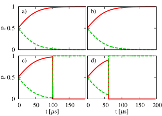
Figure 3: Exemplary singlet (green, dashed) and triplet (red, solid) probability time-evolutions for final triplet (a, b) and singlet (c, d) states, without (a, c) and with the phonon interaction (b, d).

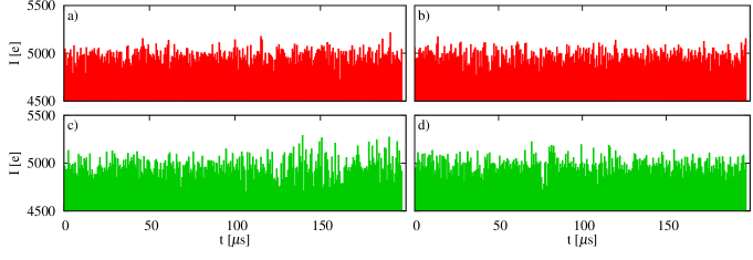
Figure 4: QPC current as a histogram of tunneling events for triplet (a, b) and singlet (c, d) states, without (a, c) and with the phonon interaction (b, d). The time interval used for the histogram is 0.66 $\mu$s.

In the following, parameters corresponding to GaAs structures are usedbarrett06 ; loss98 . The DQD energies are $U=1$ meV and $J=0.1$ meV, and the QPC bias is taken to be $V=2$ meV. Unless stated otherwise, the QPC tunneling parameters are fixed at $\mathcal{T}=4\cdot 10^{-2}$ and $\nu=9\cdot 10^{-4}$. The material parameters relevant for the calculation of the spectral density of the phonon reservoir areroszak09 $c_{L}=5100$ m/s, $c_{t}=2800$ m/s, $\epsilon_{s}=13.2$, $d=0.16$ C/m², $\sigma=-8.0$ eV and $\rho_{c}=5369$ kg/m³. Two-dimensional Gaussian single-electron wave functions were used with 170 nm full width at half maximum of the probability density, and the distance between the dots was set to $D=250$ nm. This yielded zero-temperature phonon transition rates $\gamma_{02}=1.15\cdot 10^{-3}$ ns^-1 and $\gamma_{21}=6.01\cdot 10^{-8}$ ns^-1 ($\gamma_{20}=\gamma_{12}=0$). The choice of QPC parameters corresponds to the phonon interaction being roughly $2.5$ times stronger than the QPC interaction, meaning that $\sqrt{\gamma_{02}}=2.5\nu\sqrt{V/\hbar}$.

The results presented in this and the following Section are all taken in the zero temperature limit. This is because experimental realizations of QPC measurements are performed at temperatures that do not exceed $0.1$ K, leading to extremely low phonon transition rates from lower to higher energy states.

Fig. 3 shows exemplary time evolutions of the probability of finding the DQD in a spin-singlet state (green, dashed lines) or a spin-triplet state (red, solid) for an initial equal superposition state

$$|\Psi\rangle=\frac{1}{\sqrt{2}}(|s\rangle+|t\rangle),$$ (15)

where $|t\rangle$ can be any superposition of the triplet states, Eqs (1a)-(1c), and

$$|s\rangle=\cos\frac{\theta}{2}|s_{0}\rangle+\sin\frac{\theta}{2}|s_{1}\rangle=\frac{1}{\sqrt{2}}(|\uparrow\downarrow\rangle-|\downarrow\uparrow\rangle),$$ (16)

as in Ref. [barrett06, ]. The top panels show instances where the final state is a spin-triplet (the measurement outcome was the triplet state), while the bottom-panel evolutions ended up in the spin-singlet state (the measurement outcome was the singlet state). The electron-phonon interaction is included only in the right panels; the phonon influence on coherence and localization is studied in more detail later on. As seen, regardless of the presence of the electron-phonon coupling, the continuous evolution leads to DQD localization in the triplet spin state (see Fig. 3 a, b), while for there to be a measurement of a singlet spin state, the occurrence of a quantum jump is required.

The simulation results for the QPC currents corresponding to the final singlet and triplet states are shown in Fig. 4. Even through the evolutions depicted in Fig. 3 show no clear difference between the phonon and no-phonon cases, in the phonon-free situation in Fig. 4 (left panels) a difference in the magnitude of the current fluctuations (noise) can be seen between the singlet and triplet case, while no such distinction is evident in the current when the phonon influence is included. For the realistic choice of material parameters, QPC and DQD properties, and for our choice of counting time step, the differences are relatively small, but still a period of time (after about $110$ microseconds) when the DQD electrons occupy higher energy singlet states resulting in increased current fluctuations can be seen (Fig. 4 c). When the phonon coupling is included (Fig. 4 b, d) this distinction is diminished (to the level that no time period of increased fluctuations can be seen with the “bare eye”), so the measurement effect is suppressed.

Clearly, such observations based on the informal analysis of the current noise trace are to a large extent subjective and cannot form the base for rigorous conclusions on the measurement outcome or for assessing the role of phonon-induced dissipation. In order to provide a firm ground for such a discussion, the quantitative noise characteristics, needed to fully describe phonon influence on the distinguishability of the spin-singlet and spin-triplet states in the QPC spin measurement setup, are studied in the next section.

The most obvious effect of coupling to phonons can be seen in the dynamics of coherence between singlet and triplet states expressed by the normalized amplitudes of the off-diagonal density matrix elements averaged over many realizations of single measurement simulations. The coherence time between the triplet and the $|s_{2}\rangle$ singlet states, $\tau_{s_{2}}=40.62$ $\mu$s, is over an order of magnitude longer than the other two coherence times, which are $\tau_{s_{0}}=1.03$ $\mu$s for $|s_{0}\rangle$ and $T_{s_{1}}=1.20$ $\mu$s for $|s_{1}\rangle$. Furthermore, phonon influence (Fig. 5 b) also strongly varies depending on the particular coherence in question, leaving the triplet $|s_{1}\rangle$ singlet coherence time unchanged, slightly influencing the long $|s_{2}\rangle$ coherence, the time of which is now $\tau_{s_{2}}=40.55$ $\mu$s, and cutting the coherence time of $|s_{0}\rangle$ almost by half, leaving $\tau_{s_{2}}=0.54$ $\mu$s. This is because different phonon transition rates $\gamma_{ij}$ govern the evolution of different coherences, and the rates significantly differ from one another. The coherence between a triplet and the $|s_{0}\rangle$ singlet is influenced both by the strong transition from $|s_{2}\rangle$ to $|s_{0}\rangle$ and the weaker transition from $|s_{1}\rangle$ to $|s_{2}\rangle$, hence phonon influence on the coherence times is big. The triplet–$|s_{1}\rangle$ coherence is only related to transitions from $|s_{0}\rangle$ to $|s_{2}\rangle$ and $|s_{2}\rangle$ to $|s_{1}\rangle$ which are very weak at low temperatures and do not occur at zero temperature, while the $|s_{2}\rangle$ coherence depends on the transition rates from $|s_{1}\rangle$ to $|s_{2}\rangle$ and $|s_{0}\rangle$ to $|s_{2}\rangle$, of which the first is small and the second is negligible in the low temperature range.

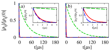
Figure 5: Normalized singlet-triplet coherences without phonon influence (a) and with phonon influence (b); $|\langle t|\rho|s_{0}\rangle|$: red solid lines, $|\langle t|\rho|s_{1}\rangle|$: green dashed lines, and $|\langle t|\rho|s_{2}\rangle|$: blue dash-dotted lines. Inset: short-time evolution.

While the dephasing rates are the most common characteristics of open system dynamics, from the point of view of the measurement process the time of localization into one of the measurement basis states (the “collapse” of the system state) is of more interest. To quantify how fast the DQD system reaches the singlet or triplet subspaces, we introduce a measure of localization analogous to the degree of localization used in the description of charge measurement goan01a . It determines the timescales on which the QPC measurement on the DQD spin states is performed. For the singlet-triplet measurement, the observable quantifying the localization is $\langle z^{2}\rangle$, where

$$z=\sum_{i}\langle t_{i}|\rho_{\mathrm{c}}|t_{i}\rangle-\sum_{i}\langle s_{i}|\rho_{\mathrm{c}}|s_{i}\rangle$$

and the averaging is performed over many simulated measurement runs. The quantity is equal to zero when the occupation of the singlet and triplet subspaces is equal and grows with the absolute value of the difference between the two occupations, reaching unity when the DQD state is either a fully triplet or a fully singlet state. Since the singlet subspace is the orthogonal complement of the triplet subspace, the degree of localization can be described using the probability of finding the system in the triplet state, which gives $z=1-2\langle t|\rho|t\rangle$. The blue dotted line in Fig. 6 shows the localization, $\langle z^{2}(t)\rangle$, for the initial equal superposition state [Eq. (15)] for which $\langle z^{2}(0)\rangle=0$. The red solid line and green dashed lines depict the evolution of localization for the same set of data, on which a post-selection into the set of measurement runs that yielded a singlet outcome (red solid) and the set that yielded a triplet outcome (green dashed) was performed. Although the localization occurs on the scale of tens of microseconds regardless of the measurement outcome, the localization is significantly faster when a singlet is measured, with localization time $\tau_{\mathrm{loc}}^{(\mathrm{s})}=20$ $\mu$s, than when triplet is measured, with localization time $\tau_{\mathrm{loc}}^{(\mathrm{t})}=46$ $\mu$s. This is because a quantum jump is needed to localize in the spin-singlet, and the occurrence of jumps shortens the localization time (as seen in Fig. 3). If no post-selection is made then localization time is $\overline{\tau}_{\mathrm{loc}}=35$ $\mu$s. As expectedmarcinowski11 , phonons have no effect on the localization times as long as they are not monitored (meaning that no measurement is performed on the phonon subsystem).

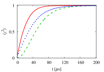
Figure 6: Localization of the DQD state with singlet post-selection (red solid line), triplet post-selection (green dashed) and with no state post-selection (blue dotted).

As can be seen from the above discussion, the phonon-induced dissipation destroys coherence but does not change the localization time, which depends only on the coupling to the measurement device. The major phonon effect, from the point of view of the measurement, is the reduction of QPC current noise in the DQD singlet state due to the phonon induced suppression of transitions to the excited singlet states which are responsible for the increased singlet current noise.

VI Noise characteristics

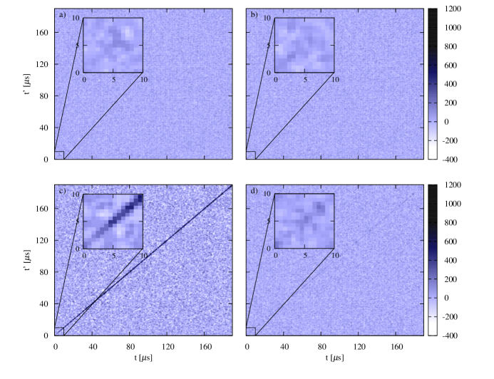
Figure 7: Current-current correlation function $G(t,t^{\prime})-G(t=t^{\prime})$ of initial equal superposition state for the triplet (a, b) and singlet (c, d) measurement outcomes without (a, c) and with the phonon interaction (b, d). Insets: Detail at short times.

Although the destructive phonon effects might already be seen in the QPC current noise of single evolutions, a general noise characteristic is much more revealingblanter01 . Fig. 7 shows the two-time maps of the current-current correlation functionblanter01 ; barrett06 ; goan01 ; stace04 ,

$$G(t,t^{\prime})=\langle I(t^{\prime})I(t)\rangle-\langle I(t^{\prime})\rangle\langle I(t)\rangle,$$ (17)

where the average $\langle...\rangle$ is taken over $\sim 5000$ measurement runs (the small-scale fluctuations in the maps are due to the finite number of runs). The strongly peaked values of the current-current correlation function for $t=t^{\prime}$ are not shown on the maps for the sake of clarity. The initial state is chosen to be the equal superposition state of Eq. (15). In the top panels (Fig. 7 a, b), the correlation function for post-selected spin-triplet measurement outcomes is shown, while in the bottom panels (Fig. 7 c, d) the post-selected spin-singlet outcomes are depicted. Again, the left panels (Fig. 7 a, c) correspond to the no-phonon case and the right panels (Fig. 7 b, d) correspond to zero-temperature phonons. When the system reaches its steady state, the correlation function no longer depends on the two times $t$ and $t^{\prime}$, but is a function only of $\tau=t^{\prime}-t$. As can be seen, regardless of the presence of phonons, the QPC current noise is Poissonian (meaning that there are no correlations present for $t\neq t^{\prime}$) when the DQD is in the triplet state. In the singlet case, current-current correlations are present for small time differences $\tau$, leading to the appearance of the diagonal line (of a finite width) on the lower left map. In the presence of phonons, these correlations are strongly suppressed due to phonon processes that preclude long intervals of occupation of excited singlet states, and the visibility of the diagonal line is much worse (lower right).

The insets on each map of Fig. 7 contain an enlargement of the area corresponding to small $t$ and $t^{\prime}$, when the system has not yet localized in either a singlet or a triplet steady state. On the scale of several microseconds (consistent with the localization time shown in Fig. 6), we observe small correlations in the upper panels which then disappear as the DQD state approaches the purely triplet state. On the lower panels we can observe the finite time over which the correlations build up, corresponding to a decreased visibility of the correlation feature before the DQD subsystem localizes in the singlet steady state.

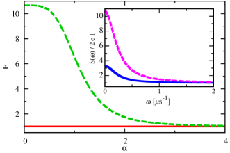
Figure 8: Steady state Fano factor for the QPC current as a function of the relative strength of the electron-phonon interaction for singlet (green dashed line) and triplet states (red solid). Inset: Normalized singlet steady state noise power spectra of the QPC detector current without (violet dashed line) and with electron-phonon interaction (blue solid), $\alpha=1.5$.

To quantify the influence of phonon effects on the measurement scheme and its dependence on the ratio between the DQD-QPC interaction and the electron-phonon coupling we use the Fano factorfano47 ; blanter01 ; flindt10 ; roszak12 . It is a widely used noise measure, defined as the zero-frequency shot noise power normalized to Poissonian shot noise power, $F={S(0)}/{2e\bar{I}}$, where $\bar{I}$ is the mean current. The QPC noise power spectrum for steady states is given by $S(\omega)=2\int_{\infty}^{\infty}\mathrm{d}\tau G(\tau)e^{-i\omega\tau}$, where the current-current correlation function, which has been introduced in Eq. (17), now only depends on $\tau=t^{\prime}-t$. Following Refs [goan01, ; barrett06, ] we can calculate the correlation functions for singlet and triplet steady states,

$$G^{(t/s)}(\tau) = e^{2}\left[\mathrm{Tr}\{\sum_{i,j}C_{j}[e^{\mathcal{L}(\tau-\Delta t)}C_{i}\rho^{(t/s)}_{\infty}C_{i}^{\dagger}]C_{j}^{\dagger}\}\right.$$ (18)

$$-\mathrm{Tr}\{\sum_{i}C_{i}\rho^{(t/s)}_{\infty}C_{i}^{\dagger}\}^{2}$$

$$+\left.\mathrm{Tr}\{\sum_{i}C_{i}\rho^{(t/s)}_{\infty}C_{i}^{\dagger}\}\delta(\tau)\right].$$

Spectra for the different measurement outcomes can be found by substituting the appropriate steady states: the singlet state is given by Eq. (III) and $\rho_{\infty}^{(t)}=|t\rangle\langle t|$.

Fig. 8 shows the singlet and triplet Fano factor curves as a function of the relative coupling strengths of the DQD to the phonon reservoir and to the QPC. For the sake of realism it is the tunneling parameters of the QPC which are changed, while the electron-phonon interaction is kept at a value corresponding to realistic gate defined QDs (see end of Section III and beginning of Section V). The scaling parameter $\alpha=\frac{\mathcal{T}_{0}}{\mathcal{T}}=\frac{\nu_{0}}{\nu}$, with $\mathcal{T}_{0}=0.1$ and $\nu_{0}=2.25\cdot 10^{-3}$, is chosen in such way that $\alpha=1$ corresponds to the situation when the interaction with phonons is roughly the same strength as the interaction with the QPC; this means that $\sqrt{\gamma_{02}}=\nu_{0}\sqrt{V/\hbar}$. As can be seen, the phonons dominate at large $\alpha$ (small QPC current) leading to a suppression of the noise difference and breaking of the measurement scheme, while for large currents their effect is negligible. Note that the results discussed earlier in this paper correspond to the QPC interaction strength $\alpha=2.5$. Even though the phonon-induced suppression of the spin-singlet Fano factor at this moderate value of the scaling parameter is small, the effects seen in Figs 3 - 7 are already non-negligible. The normalized singlet steady state noise power as a function of frequency is shown in the inset of Fig. 8. The blue solid line corresponds to $\alpha=1.5$, while the violet dashed line depicts the no-phonon situation at the same QPC current values. As can be seen, phonon-interactions lead to noise damping for the whole noise power spectrum. On the other hand, the width of the noise power spectrum $S(\omega)$ does not change when the phonon effects are included. This obviously means that the width of the corresponding feature in the correlation function $G(\tau)$ is insensitive to phonons. Since this width sets the minimum time scale over which the measurement has to be continued in order to extract the spectral characteristics shown in Fig. 8, this leads to the conclusion that also this measurement-related time scale is not affected by phonon-induced decoherence.

VII Conclusions

We have studied phonon-influence on the QPC measurement of two-electron DQD spin states, relying on different characteristics of the resulting QPC current noise. We have shown that although phonons destroy the singlet-triplet coherence, they do not affect the localization of the DQD into the measurement basis and therefore do not influence this contribution to the measurement time. Also the time necessary to establish the spectral properties of the noise, which is on the order of the correlation time, does not change when carrier-phonon coupling is included. Nonetheless, phonons do disturb the measurement by impeding the distinguishability of the spin-singlet and spin-triplet configurations. This is due to the phonon-induced suppression of singlet-singlet transitions between low and high energy states which are responsible for the differences in the noise observed for the triplet and singlet spin symmetries. This is reflected, in particular, by the reduced amplitude of the singlet-related feature in the noise power spectrum and the suppressed super-Poissonian character of the Fano factor.

We have found that the perturbing phonon effects with respect to the measurement distinguishability at moderate relative strengths of the DQD-QPC and electron-phonon couplings are already non-negligible. Furthermore, the electron-phonon interaction can lead to complete indistinguishability of the two spin configurations, if it is strong enough compared to the DQD-QPC coupling. This means that the mechanism may render the measurement scheme completely useless, while it does not impose a lengthening of the times of the measurement-induced localization into the triplet and singlet subspaces.

VIII Acknowledgments

We are very grateful to Ryszard Buczko and Jan Mostowski for discussions which inspired this work, and to Tomáš Novotný and Mateusz Kwaśnicki for helpful discussions relating to noise characteristics. This work was supported in parts by the TEAM programme of the Foundation for Polish Science, co-financed from the European Regional Development Fund and by the Polish NCN Grant No. 2012/05/B/ST3/02875. The calculations were carried out in the Wrocław Centre for Networking and Supercomputing (http://www.wcss.wroc.pl), grant no. 203.

References

- (1) D. Loss and D. P. DiVincenzo, Phys. Rev. A 57, 120 (1998).
- (2) K. C. Nowack, F. H. L. Koppens, Y. V. Nazarov, and L. M. K. Vandersypen, Science 318, 1430 (2007).
- (3) A. Greilich, S. E. Economou, S. Spatzek, D. R. Yakovlev, D. Reuter, A. D. Wieck, T. L. Reinecke, and M. Bayer, Nature Physysics 5, 262 (2009).
- (4) N. Y. Kim, K. Kusudo, C. Wu, N. Masumoto, A. Loffler, S. Hofling, N. Kumada, L. Worschech, A. Forchel, and Y. Yamamoto, Nature Physics 7, 681 (2011).
- (5) W. A. Coish and D. Loss, Phys. Rev. B 72, 125337 (2005).
- (6) A. Johnson, J. Petta, J. Taylor, A. Yacoby, M. Lukin, C. Marcus, M. Hanson, and A. Gossard, Nature 435, 925 (2005).
- (7) A. Pfund, I. Shorubalko, K. Ensslin, and R. Leturcq, Phys. Rev. Lett. 99, 036801 (2007).
- (8) D. Stepanenko, M. Rudner, B. I. Halperin, and D. Loss, Phys. Rev. B 85, 075416 (2012).
- (9) B. M. Maune, M. G. Borselli, B. Huang, T. D. Ladd, P. W. Deelman, K. S. Holabird, A. A. Kiselev, I. Alvarado-Rodriguez, R. S. Ross, A. E. Schmitz, M. Sokolich, C. A. Watson, M. F. Gyure, and A. T. Hunter, Nature 481, 344 (2012).
- (10) J. Levy, Phys. Rev. Lett. 89, 147902 (2002).
- (11) J. R. Petta, A. C. Johnson, J. M. Taylor, E. A. Laird, A. Yacoby, M. D. Lukin, C. M. Marcus, M. P. Hanson, and A. C. Gossard, Science 309, 2180 (2005).
- (12) J. M. Taylor, J. R. Petta, A. C. Johnson, A. Yacoby, C. M. Marcus, and M. D. Lukin, Phys. Rev. B 76, 035315 (2007).
- (13) M. D. Shulman, O. E. Dial, S. P. Harvey, H. Bluhm, V. Umansky, and A. Yacoby, Science 336, 202 (2012).
- (14) C. Beenakker and H. van Houten, Solid State Physics 44, 1 (1991).
- (15) S. D. Barrett and T. M. Stace, Phys. Rev. B 73, 075324 (2006).
- (16) T. M. Stace, S. D. Barrett, H.-S. Goan, and G. J. Milburn, Phys. Rev. B 70, 205342 (2004).
- (17) M. A. Nielsen and I. L. Chuang, Quantum Computation and Quantum Information (Cambridge University Press, Cambridge, 2000).
- (18) D. V. Averin and E. V. Sukhorukov, Phys. Rev. Lett. 95, 126803 (2005).
- (19) T. Meunier, I. T. Vink, L. H. W. van Beveren, F. H. L. Koppens, H. P. Tranitz, W. Wegscheider, L. P. Kouwenhoven, and L. M. K. Vandersypen, Phys. Rev. B 74, 195303 (2006).
- (20) M. C. Rogge, B. Harke, C. Fricke, F. Hohls, M. Reinwald, W. Wegscheider, and R. J. Haug, Phys. Rev. B 72, 233402 (2005).
- (21) C. Barthel, D. J. Reilly, C. M. Marcus, M. P. Hanson, and A. C. Gossard, Phys. Rev. Lett. 103, 160503 (2009).
- (22) M. C. Cassidy, A. S. Dzurak, R. G. Clark, K. D. Petersson, I. Farrer, D. A. Ritchie, and C. G. Smith, Appl. Phys. Lett. 91, 222104 (2007).
- (23) J. Bylander, T. Duty, and P. P.Delsing, Nature 434, 361 (2005).
- (24) J. M. Elzerman, R. Hanson, L. H. Willems van Beveren, B. Witkamp, L. M. K. Vandersypen, and L. P. Kouwenhoven, Nature 430, 431 (2004).
- (25) Ł. Marcinowski, M. Krzyżosiak, K. Roszak, P. Machnikowski, R. Buczko, and J. Mostowski, Acta Phys. Pol. A 119, 640 (2011).
- (26) A. Grodecka, P. Machnikowski, and J. Förstner, Phys. Rev. B 78, 085302 (2008).
- (27) D. J. Reilly, C. M. Marcus, M. P. Hanson, and A. C. Gossard, Applied Physics Letters 91, 162101 (2007).
- (28) K. Roszak and P. Machnikowski, Phys. Rev. B 80, 195315 (2009).
- (29) S. A. Gurvitz and Y. S. Prager, Phys. Rev. B 53, 15932–15943 (1996).
- (30) H.-S. Goan and G. J. Milburn, Phys. Rev. B 64, 235307 (2001).
- (31) B. Krummheuer, V. M. Axt, and T. Kuhn, Phys. Rev. B 65, 195313 (2002).
- (32) A. Vagov, V. M. Axt, and T. Kuhn, Phys. Rev. B 66, 165312 (2002).
- (33) A. Vagov, V. M. Axt, and T. Kuhn, Phys. Rev. B 67, 115338 (2003).
- (34) A. Grodecka, L. Jacak, P. Machnikowski, and K. Roszak, in Quantum Dots: Research Developments, edited by P. A. Ling (Nova Science, NY, 2005), p. 47.
- (35) K. Roszak, P. Horodecki, and R. Horodecki, Phys. Rev. A 81, 042308 (2010).
- (36) G. D. Mahan, Many-Particle Physics (Kluwer, New York, 2000).
- (37) G. D. Mahan, in Polarons in Ionic Crystals and Polar Semiconductors, edited by J. T. Devreese (North-Holland, Amsterdam, 1972).
- (38) K. Roszak, A. Grodecka, P. Machnikowski, and T. Kuhn, Phys. Rev. B 71, 195333 (2005).
- (39) H.-P. Breuer and F. Petruccione, The Theory of Open Quantum Systems (Oxford University Press, Oxford, 2002).
- (40) S. Gustavsson, I. Shorubalko, R. Leturcq, S. Schön, and K. Ensslin, Appl. Phys. Lett. 92, 152101 (2008).
- (41) P. Meystre and M. Sargent, Elements of Quantum Optics (Springer-Verlag, Berlin, 2007).
- (42) H.-S. Goan, G. J. Milburn, H. M. Wiseman, and H. Bi Sun, Phys. Rev. B 63, 125326 (2001).
- (43) H. M. Wiseman, D. W. Utami, H. B. Sun, G. J. Milburn, B. E. Kane, A. Dzurak, and R. G. Clark, Phys. Rev. B 63, 235308 (2001).
- (44) C. Gardiner and P. Zoller, Quantum Noise (Springer, Berlin, 2004).
- (45) Y. M. Blanter and M. Büttiker, Physics Reports 336, 1 (2000).
- (46) U. Fano, Phys. Rev. 72, 26 (1947).
- (47) C. Flindt, T. Novotný, A. Braggio, and A.-P. Jauho, Phys. Rev. B 82, 155407 (2010).
- (48) N. Ubbelohde, K. Roszak, F. Hohls, N. Maire, R. J. Haug, and T. Novotny, Sci. Rep. 2, 374 (2012).