Exploiting Opportunistic Physical Design in Large-scale Data Analytics

Abstract

Big data analytical systems, such as MapReduce, perform aggressive materialization of intermediate job results in order to support fault tolerance. When jobs correspond to exploratory queries submitted by data analysts, these materializations yield a large set of materialized views that typically capture common computation among successive queries from the same analyst, or even across queries of different analysts who test similar hypotheses. We propose to treat these views as an opportunistic physical design and use them for the purpose of query optimization. We develop a novel query-rewrite algorithm that addresses the two main challenges in this context: how to reason about views that contain UDFs (a common feature in big data analytics), and how to search the large space of rewrites. To do this, we first develop a semantic UDF model that captures an important class of UDFs for big data analysis: MapReduce UDFs containing arbitrary code. The model enables effective reuse of previous results generated by UDFs. We then present a rewrite algorithm, inspired by nearest-neighbor searches in metric spaces, that provably finds the minimum-cost rewrite under certain assumptions. An extensive experimental study on real-world datasets using our prototype based on Hive shows that our approach results in dramatic performance improvements for complex big data analysis queries — reducing total execution time over 60% on average and up to an order of magnitude.

1 Introduction

Data analysts have the crucial task of analyzing the ever increasing volume of data that modern organizations collect in order to produce actionable insights. As expected, this type of analysis on big data is highly exploratory in nature and involves an iterative process: the data analyst starts with an initial query over the data, examines the results, then reformulates the query and may even bring in additional data sources, and so on. Typically, these queries involve sophisticated, domain-specific operations that are linked to the type of data and the purpose of the analysis, e.g., performing sentiment analysis over tweets or computing network influence. Because a query is often revised multiple times in this scenario, there can be significant overlap between queries. There is an opportunity to speed up these explorations by reusing previous query results either from the same analyst or from different analysts performing a related task.

MapReduce (MR) has become a de-facto tool for this type of analysis. It offers scalability to large datasets, easy incorporation of new data sources, the ability to query right away without defining a schema up front, and extensibility through user-defined functions (UDFs). Analyst queries are often written in a declarative query language, e.g., HiveQL or PigLatin, which are automatically translated to a set of MR jobs. Each MR job involves the materialization of intermediate results (the output of mappers, the input of reducers and the output of reducers) for the purpose of failure recovery. A typical Hive or Pig query will spawn a multi-stage job that will involve several such materializations. We refer to these execution artifacts as opportunistic materialized views.

We propose to treat these views as an opportunistic physical design and to use them to rewrite queries. The opportunistic nature of our technique has several nice properties: the materialized views are generated as a by-product of query execution, i.e., without additional overhead; the set of views is naturally tailored to the current workload; and, given that large-scale analysis systems typically execute a large number of queries, it follows that there will be an equally large number of materialized views and hence a good chance of finding a good rewrite for a new query. Our results indicate the savings in query execution time can be dramatic: a rewrite can reduce execution time by up to an order of magnitude.

Rewriting a query using views in the context of MR involves a unique combination of technical challenges. First, the queries and views almost certainly contain UDFs, thus query rewriting requires some semantic understanding of UDFs. These MR UDFs for big data analysis are composed of arbitrary user-code and may involve a sequence of MR jobs. Second, any query rewriting algorithm that can utilize UDFs now has to contend with a potentially large number of operators since any UDF can be included in the rewriting process. Third, there can be a large search space of views to consider for rewriting due to the large number of materialized views in the opportunistic physical design, since they are almost free to retain (storage permitting).

Recent methods to reuse MR computations such as ReStore [5] and MRShare [16] lack any semantic understanding of execution artifacts and can only reuse/share cached results when execution plans are syntactically identical. We strongly believe that any truly effective solution will have to a incorporate a deeper semantic understanding of cached results and “look into” the UDFs as well.

Contributions. In this paper we present a novel query-rewrite algorithm that targets the scenario of opportunistic materialized views in an MR system with queries that contain UDFs. We propose a UDF model that has a limited semantic understanding of UDFs, yet enables effective reuse of previous results. Our rewrite algorithm employs techniques inspired by spatial databases (specifically, nearest-neighbor searches in metric spaces [9]) in order to provide a cost-based incremental enumeration of the huge space of candidate rewrites, generating the optimal rewrite in an efficient manner. Specifically, our contributions can be summarized as follows:

• A gray-box UDF model that is simple but expressive enough to capture a large class of MR UDFs that includes many common analysis tasks. The UDF model further provides a quick way to compute a lower-bound on the cost of a potential rewrite given just the query and view definitions. We provide the model and the types of UDFs it admits in Sections 3–4.

• A rewriting algorithm that uses the lower-bound to (a) gradually explode the space of rewrites as needed, and (b) only attempts a rewrite for those views with good potential to produce a low-cost rewrite. We show that the algorithm produces the optimal rewrite as well as finds this rewrite in a work-efficient manner, under certain assumptions. We describe this further in Sections 6–7.

• An experimental evaluation showing that our methods provide execution time improvements of up to an order of magnitude using real-world data and realistic complex queries containing UDFs. The execution time savings of our method are due to moving much less data and avoiding the high expense of re-reading data from raw logs when possible. We describe this further in Section 8.

2 Preliminaries

Here we present the architecture of our system and briefly describe its components and how they interact, followed by our notations and problem definition.

2.1 System Architecture

Figure 1 provides a high level overview of our system and its components. Our system is built on top of Hive, and queries are written in HiveQL. Queries are posed directly over log data stored in HDFS. In Hive, MapReduce UDFs are given by the user as a series of Map or Reduce jobs containing arbitrary user code expressed in a supported language such as Java, Perl, Python, etc. To reduce execution cost, our system automatically rewrites queries based on the existing views. A query execution plan in Hive consists of a series of MR jobs, and each MR job materializes its output to HDFS. As Hive lacks a mature query optimizer and cannot cost UDFs, we implemented an optimizer based on the cost model from [18] and extended it to cost UDFs, as described later in Section 4.2.

During query execution, all by-products of query processing (i.e., the intermediate materializations) are retained as opportunistic materialized views. These views are stored in the system (space permitting) as the opportunistic physical design.

The materialized view metadata store contains information about the materialized views currently in the system such as the view definitions and standard data statistics used in query optimization. For each view stored, we collect statistics by running a lightweight Map job that samples the view’s data. This constitutes a small overhead, but as we show experimentally in Section 8, this time is a small fraction of query execution time.

The rewriter, presented in Section 6, uses the materialize view metadata store to rewrite queries based on the existing views. To facilitate this, our optimizer generates plans with two types of annotations on each plan node: (1) the logical expression of its computation (Section 3.2) and (2) the estimated execution cost (Section 4.2).

Figure 1: System diagram showing control flows.

The rewriter uses the logical expression in the annotation when searching for rewrites for each node in the plan. The expression consists of relational operators or UDFs. For each rewrite found during the search, the rewriter utilizes the optimizer to obtain an estimated cost for the rewritten plan.

2.2 Notations

$W$ denotes a plan generated by the query optimizer, which is represented as a DAG containing $n$ nodes, ordered topologically. Each node represents an MR job. We denote the $i^{th}$ node of $W$ as $\mbox{\sc node}_{i}$, $i\in[1,n]$. The plan has a single sink that computes the result of the query; under the topological order assumption the sink is $\mbox{\sc node}_{n}$. $W_{i}$ is a sub-graph of $W$ containing $\mbox{\sc node}_{i}$ and all of its ancestor nodes. We refer to $W_{i}$ as one of the rewritable targets of plan $W$. As is standard in Hive, the output of each job is materialized to disk. Hence, a property of $W_{i}$ is that it represents a materialization point in $W$, and in this way, materializations are free except for statistics collection. An outgoing edge from $\mbox{\sc node}_{k}$ to $\mbox{\sc node}_{i}$ represents data flow from $k$ to $i$. $V$ is the set of all opportunistic materialized views (MVs) in the system.

We use $\mbox{\sc Cost}(\mbox{\sc node}_{i})$ to denote the cost of executing the MR job at $\mbox{\sc node}_{i}$, as estimated by the query optimizer. Similarly, $\mbox{\sc Cost}(W_{i})$ denotes the estimated cost of running the sub-plan rooted at $W_{i}$, which is computed as $\mbox{\sc Cost}(W_{i})=\sum_{\forall\mbox{\sc node}_{k}\in W_{i}}\mbox{\sc Cost}(\mbox{\sc node}_{k})$.

We use $r_{i}$ to denote an equivalent rewrite of target $W_{i}$ iff $r_{i}$ uses only views in $V$ as input and produces an identical output to $W_{i}$, for the same database instance $D$. A rewrite $r^{*}$ represents the minimum cost rewrite of $W$ (i.e., target $W_{n}$).

2.3 Problem Definition

Given these basic definitions, we introduce the problem we solve in this paper.

Problem Statement. Given a plan $W$ for an input query $q$, and a set of materialized views $V$, find the minimum cost rewrite $r^{*}$ of $W$.

Our rewrite algorithm considers views in $V$ during the search for $r^{*}$. Since some views may contain UDFs, for the rewriter to utilize those views during its search, some understanding of UDFs is required. Next we will describe our UDF model and then present our rewrite algorithm that solves this problem.

3 UDF Model

Since big data queries frequently include UDFs, in order to reuse previous computation in our system effectively we desire a way to model MR UDFs semantically. If the system has no semantic understanding of the UDFs, then the opportunities for reuse will be limited — essentially the system will only be able to exploit cached results when one query applies the exact same UDF to the exact same input as a previous query. However, to the extent that we are able to “look into” the UDFs and understand their semantics, there will be more possibilities for reusing previous results. In this section we propose a UDF model that allows a deeper semantic understanding of MR UDFs. Our model is general enough to capture a large class of UDFs that includes classifiers, NLP operations (e.g., taggers, sentiment), text processors, social network (e.g., network influence, centrality) and spatial (e.g., nearest restaurant) operators. Of course, we do not require the developer to restrict herself to this model; rather, to the extent a query uses UDFs that follow this model, the opportunities for reuse will be increased.

3.1 Modeling a UDF

Figure 2: A UDF composed of local functions (lf₁, lf₂, $\cdots$, lf_k), showing the end-to-end transformation of input to output.

We propose a model for UDFs that allows the system to capture a UDF as a composition of local functions as shown in Figure 2, where each local function represents a map or reduce task. The nature of the MR framework is that map-reduce functions are stateless and only operate on subsets of the input, i.e., a single tuple or a single group of tuples. Hence, we refer to these map-reduce functions as local functions. A local function can only perform a combination of the following three types of operations performed by map and reduce tasks.

1. Discard or add attributes, where an added attribute and its values may be determined by arbitrary user code

2. Discard tuples by applying filters, where the filter predicates may be performed by arbitrary user code

3. Perform grouping of tuples on a common key, where the grouping operation may be performed by arbitrary user code

The end-to-end transformation of a UDF is obtained by composing the operations performed by each local function lf in the UDF. Our model captures the fine-grain dependencies between the input and output tuples in the following way.

The UDF input is modeled as $(A,F,K)$ where $A$ is the set of attributes, $F$ is set of filters previously applied to the input, and $K$ is the current grouping of the input, which captures the keys of the data. The output is modeled as $(A^{\prime},F^{\prime},K^{\prime})$ with the same semantics. Our model describes a UDF as the transformation from $(A,F,K)$ to $(A^{\prime},F^{\prime},K^{\prime})$ as performed by a composition of local functions using operation types (1) (2) (3) above. Figure 2 shows how to semantically model a UDF that takes any arbitrary input represented as $A,F,K$ and applies local functions to produce an output that is represented as $A^{\prime},F^{\prime},K^{\prime}$. Additionally, for any new attribute produced by a UDF (in the output schema $A^{\prime}$), its dependencies on the input (in terms of $A,F,K$) and are recorded as a signature along with the unique UDF-name.

Figure 3: UDF_FOODIES a) implementation composed of two local functions, b) UDF model showing the end-to-end transformation of input to output.

As an example, consider UDF_FOODIES that applies a food sentiment classifier on tweets to identify users that tweet positively about food. An abbreviated HiveQL definition of the UDF is given in Figure 3(a) that invokes the following two local functions lf₁ and lf₂ written in a high-level language (Perl in this example). lf₁: For each (user_id, tweet_text), apply the food sentiment classifier function that computes a sentiment value for each tweet about food. lf₂: For each user_id, compute the sum of the sentiment values to produce sent_sum, then filter out users with a total score greater than a threshold.

The two local functions correspond to arbitrary user code that perform complex text processing tasks such as parsing, word-stemming, entity tagging, and word sentiment scoring. Yet, the UDF model succinctly captures the end-to-end transformation of this complex UDF as shown in Figure 3(b). In the figure, the end-to-end transformation of UDF_FOODIES is captured by recording the changes made to the input $A$, $F$ and $K$ by the UDF functions that produces $A^{\prime}$, $F^{\prime}$ and $K^{\prime}$ using a simple notation. Furthermore, for the new attribute sent_sum in $A^{\prime}$, its dependencies on the subset of the inputs are recorded. We provide a more concrete example of the application of the UDF model in a HIVEQL query in Section 3.2. In this way, the model encodes arbitrary user-code representing a sequence of MR jobs, by only capturing its end-to-end transformations.

Our approach represents a gray-box model for UDFs, giving the system a limited view of the UDF’s functionality yet allowing the system to understand the UDF’s transformations in a useful way. In contrast, a white-box approach requires a complete understanding of how the transformations are performed, imposing significant overhead on the system. While with a black-box model, there is very little overhead but no semantic understanding of the transformations, limiting the opportunity to reuse any previous results.

3.2 Applying the UDF Model and Annotations

Figure 4: (a) Example query to obtain prolific foodies, and (b) corresponding annotated query plan.

Having presented our model for UDFs, we now show how to use it to annotate a query plan that contains both UDFs and relational operators. In Figure 4(a), we show a query that uses Twitter data to identify prolific users who talk positively about food (i.e., “foodies”). The query is expressed in a simplified representation of HiveQL and applies UDF_FOODIES from Figure 3(a) that computes a food sentiment score (sent_sum) per user based on each user’s tweets.

The HiveQL query is converted to an annotated plan as shown in Figure 4(b) by utilizing the UDF model of UDF_FOODIES as given in Figure 3(b). In addition to modeling UDFs, the three operations (denoted as 1, 2, 3 above) can also be used to characterize standard relational operators such as select (2), project (1), join (2,3), group-by (3), and aggregation (3,1). Joins in MR can be performed as a grouping of multiple relations on a common key (e.g., co-group in Pig) and applying a filter. Similarly, aggregations are a re-keying of the input (reflected in $K^{\prime}$) producing a new output attribute (reflected in $A^{\prime}$). These $A,F,K$ annotations can be applied to both UDFs and relational operations, enabling the system to automatically annotate every edge in the query plan.

Figure 4(b) shows the input to the UDF is modeled as $\langle A$={user_id, tweet_id, tweet_text}, $F$=$\emptyset$, $K$=tweet_id$\rangle$. The output is $\langle A^{\prime}$={user_id, sent_sum}, $F^{\prime}$=sent_sum > 0.5, $K^{\prime}$=user_id$\rangle$. UDF_FOODIES produces the new attribute sent_sum whose dependencies are recorded (i.e., signature) as: $\langle A$={user_id, tweet_text}, $F$=$\emptyset$, $K$=tweet_id, udf_name=UDF_FOODIES$\rangle$. Lastly, as shown in Figure 4(b), the output of the UDF ($A^{\prime},F^{\prime},K^{\prime}$) forms one input to the subsequent join operator, which in turn transforms its inputs to the final result.

This example shows how a query containing a UDF with arbitrary user code can be semantically modeled. The $A,F,K$ properties are straightforward and can be provided as annotations by the UDF creator with minimal overhead, or alternatively they may be automatically deduced via some code analysis method such as [10]. The annotations for each UDF are only provided once, i.e, the first time the UDF is added to the system.

While this model may appear limited in its expressiveness, in practice it captures a large class of common UDFs. As an example, we performed an empirical analysis of two real-world UDF libraries, Piggybank [19] and DataFu [4]. Our model captures 90% of the UDFs examined: 16 out of 16 Piggybank UDFs, and 30 out of 35 DataFu UDFs detailed in [3]. Two classes of UDFs not captured by our model are: (a) non-deterministic UDFs such as those that rely on runtime properties (e.g., current time, random, and stateful UDFs) and (b) UDFs where the output schema itself is dependent upon the input data values (e.g., pivot UDFs, contextual UDFs).

4 Using the UDF Model to Perform Rewrites

Our goal is to leverage previously computed results when answering a new query. The UDF model aids us in achieving this goal in three ways: First, it provides a way to check for equivalence. Second, it aids in the costing of UDFs. Third, it provides a lower-bound on the cost of a potential rewrite.

4.1 Equivalence Testing

The system searches for rewrites using existing views and can test for semantic equivalence in terms of our model using the properties $A$, $F$, and $K$. We consider a query and a view to be equivalent if they have identical $A$, $F$ and $K$ properties. If a query and a view are not equivalent, our system considers applying transformations (sometimes referred to as compensations) to make the existing view equivalent to the query.

Here we develop the mechanics to test if a query $q$ (i.e., a target in the annotated plan) can be rewritten using an existing view $v$. Query $q$ can be rewritten using view $v$ if $v$ contains $q$. Checking containment is a known hard problem [11] even for conjunctive queries, hence we make a first guess that only serves as a quick conservative approximation of containment. This conservative guess allows us to focus computational efforts toward checking containment on the most promising previous results and avoid wasting computational effort on less promising ones.

We provide a function $\mbox{\sc GuessComplete}(q,v)$ that performs this heuristic check. $\mbox{\sc GuessComplete}(q,v)$ takes an optimistic approach, representing a guess that a complete rewrite of $q$ exists using only $v$. This guess requires the following necessary conditions as described in [8] (SPJ) and [6] (SPJGA) that a view must satisfy to participate in a complete rewrite of $q$.

1. $v$ contains all attributes required by $q$; or contains all necessary attributes to produce those attributes in $q$ that are not in $v$

2. $v$ contains weaker selection predicates than $q$

3. $v$ is less aggregated than $q$

The function $\mbox{\sc GuessComplete}(q,v)$ performs these checks and returns true if $v$ satisfies the properties i–iii with respect to $q$. Note these conditions under-specify the requirements for determining that a valid rewrite exists, as they are necessary but not sufficient conditions. Thus the guess may result in a false positive, but will never result in a false negative. The purpose of $\mbox{\sc GuessComplete}(q,v)$ is to provide a quick way to distinguish between views that can possibly produce a rewrite from views that cannot. Since rewriting is an expensive process, this helps to avoid examining views that cannot produce valid rewrites.

4.2 Costing a UDF

Given that our goal is to find a low cost rewrite for queries containing UDFs, we require a method of costing a MapReduce UDF. We define the cost of a UDF as the sum of the cost of its local functions. Estimating the cost of a local function that performs any of the three operation types is complicated by two factors:

1. Each operation type is performed by arbitrary user code, and they could be of varying complexity. For instance, consider an NLP sentence tagger and a simple word-counter function. Although both functions perform the same operation type (discard or add attributes), they can have significantly different computational costs.

2. There could be multiple operation types performed in the same local function, making it unrealistic to develop a cost model for every possible local function. So, we desire a conservative way to estimate the cost of a local function that applies a sequence of operations without knowing how these operations interact with each other inside the local function.

Developing an accurate cost model is a general problem for any database system. In our framework, the importance of the cost model is only in guiding the exploration of the space of rewrites. For this reason, we appeal to an existing cost model from the literature [18], but slightly modify it to be able to cost UDFs. However, an improved cost model can be plugged in as it becomes available. Here, we develop a simple cost model that works well in practice. To this end, we extend the “data only” cost model in [18] in a limited way so that we are able to produce cost estimates for UDFs. Although this results in a rough cost estimate, experimentally we show that our cost model is effective in producing low cost rewrites (Section 8).

Recall that UDFs are composed of local functions, where each local function must be performed by a map task or reduce task. The cost model in [18] accounts for the “data” costs (read/write/shuffle), and we augment it in a limited way to account for the “computational” cost of local functions. Since a UDF can encompass multiple jobs, we express the cost of each job as the sum of: the cost to read the data and apply a map task ($C_{m}$), the cost of sorting and copying ($C_{s}$), the cost to transfer data ($C_{t}$), the cost to aggregate data and apply a reduce task ($C_{r}$), and finally the cost to materialize the output ($C_{w}$). Using this as a generic cost model, we first describe our approach toward solving (a) by assuming that each local function only performs one instance of a single operation type. Then we describe our approach for (b).

For (a) we model the cost of the three operation types rather than each local function. This gives a baseline calibration step for each operation type. As noted, there can be a high variance in computational costs of local functions that perform the same operation type. To remedy this, the computation cost of every local function (assuming for now it only performs a single operation type), is initially set to the cost provided by the generic model. For a local function that is computationally expensive, we scale-up its cost by applying a scalar multiplier to the generic cost of $C_{m}$ and $C_{r}$. Identifying this scalar value is a one-time process that we obtain by running a micro-job on a small sample of its input data, performed only the first time the UDF is added to the system.

For (b), since a local function performs an arbitrary sequence of operations of any type, it is difficult to estimate its cost. This would require knowing how the different operations actually interact with one another as in a white-box approach. For this reason we desire a conservative way to estimate the cost of a local function, which we do by appealing to the following property of any cost model performing a set $S$ of operations.

Definition 1

Non-subsumable cost property: Let $\mbox{\sc Cost}(S,D)$ be defined as the total cost of performing all operations in $S$ on a database instance $D$. The cost of performing $S$ on a database instance $D$ is at least as much as performing the cheapest operation in $S$ on $D$.

$$\mbox{\sc Cost}(S,D)\geq\min(\mbox{\sc Cost}(x,D),\forall x\in S)$$

The gray-box model of the UDFs only captures enough information about the local functions to provide a cost corresponding to the least expensive operation performed on the input. We cannot use the most expensive operation in $S$ (i.e., $\max(\mbox{\sc Cost}(x,D),\forall x\in S)$), since this requires $\mbox{\sc Cost}(S^{\prime},D)\leq\mbox{\sc Cost}(S,D)$, where $S^{\prime}\subseteq S$. The “max” requirement is difficult to meet in practice, which we prove using a simple counter-example. Suppose $S$ contains a filter with high selectivity, and a group-by with higher cost than the filter when considering these operations independently on database $D$. Let $S^{\prime}$ contain only group-by. Suppose that applying the filter before group-by results in few or no tuples streamed to group-by. Then applying group-by can have nearly zero cost and it is plausible that $\mbox{\sc Cost}(S^{\prime},D)>\mbox{\sc Cost}(S,D).\qquad\blacksquare$

We utilize the non-subsumable cost property in the following way. A local function that performs multiple operation types $t$ is given an initial cost corresponding to the generic cost of applying the cheapest operation type in $t$ on its input data. This initial value can then be scaled-up as described previously in our solution for (a).

4.3 Lower-bound on Cost of a Potential Rewrite

Now that we have a quick way to determine if a view $v$ can potentially produce a rewrite for query $q$, and a method for costing UDFs, we would like to compute a quick lower bound on the cost of any potential rewrite – without having to actually find a valid rewrite, which is computationally hard. To do this, we will utilize our UDF model and the non-subsumable cost property when computing the lower-bound. The ability to quickly compute a lower-bound is a key feature of our approach.

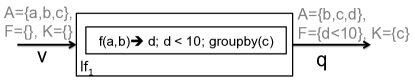
Figure 5: Synthesized UDF to perform the fix between a view $v$ and a query $q$.

As an example of computing the lower bound, we show a view $v$ and a query $q$ in Figure 5 annotated using the model. Suppose that $v$ is given by attributes $\{a,b,c\}$ with no applied filters or grouping keys. Now, suppose that $q$ is given by $\{b,c,d\}$, has a filter $d<10$, and has key $c$, where attribute $d$ is computed using $a$ and $b$, which happen to be present in $v$. It is clear that $v$ is guessed to be complete with respect to $q$ because $v$ has the required attributes to produce $q$ and $v$ has weaker filters and grouping keys (i.e., is less aggregated) than $q$. Note that the guess implies it may not be complete since it may be possible that the application of the grouping on $c$ may remove $a$ and $b$, rendering the creation of $d$ not possible. However, since it passes the $\mbox{\sc GuessComplete}(q,v)$ test, we can then compute what we term the fix for $v$ with respect to $q$. Using the UDF model, the representation of $q$ in terms of $A,F,K$ can be compared with that of $v$ in terms of $A,F,K$. To compute the fix, we only take the set difference between the attributes, filters, and group-bys ($A,F,K$), which is straightforward and simple to compute. In Figure 5, the fix for $v$ with respect to $q$ is given by: a new attribute $d$; a filter $d<10$; and group-by on $c$.

To produce a valid rewrite we need to find a sequence of local functions that “perform” the fix; these are the operations that when applied to $v$ will produce $q$. As this a known hard problem, we synthesize a hypothetical UDF comprised of a single local function that applies all operations in the fix. The cost of this synthesized UDF, which serves as an initial stand-in for a potential rewrite should one exist, is obtained using our UDF cost model. This cost corresponds to the lower-bound of any valid rewrite $r$ — by the non-subsumable cost property, the computational cost of this single local function is the cost of the cheapest operation in the fix. The benefit of the lower-bound is that it lets us cost views by their potential ability to produce a low-cost rewrite, without having to expend the computational effort to actually find one. Later we show how this allows us to consider views that are “more promising” to produce a low-cost rewrite before the “less promising” views are considered.

We define an optimistic cost function $\mbox{\sc OptCost}(q,v)$ that computes this lower-bound on any rewrite $r$ of query $q$ using view $v$ only if $\mbox{\sc GuessComplete}(q,v)$ is true. Otherwise $v$ is given OptCost of $\infty$, since in this case it cannot produce a complete rewrite, and hence the Cost is also $\infty$. The properties of $\mbox{\sc OptCost}(q,v)$ are that it is very quick to compute and

$$\mbox{\sc OptCost}(q,v)\leq\mbox{\sc Cost}(r).$$

When searching for the optimal rewrite $r^{*}$ of $W$, we use OptCost to enumerate the space of the candidate views based on their cost potential, as we describe in the next section. This is inspired by nearest neighbor finding problems in metric spaces where computing distances between objects can be computationally expensive, thus preferring an alternate distance function (e.g., OptCost) that is easy to compute with the desirable property that it is always less than or equal to the actual distance.

5 Problem Overview for Rewriting Queries Containing UDFs

Our UDF model enables reuse of views to improve query performance even when queries contain complex functions. However, reusing an existing view when rewriting a query with any arbitrary UDF requires the rewrite process to consider all UDFs in the system. Given that the system will likely have many users who write a lot of queries and UDFs, including all these UDFs in the rewrite process makes searching for the optimal rewrite impractical for any realistic workload and number of views. This is because the search space for finding a rewrite is exponential in both 1) the number of views in $V$ and 2) the operations considered by the rewrite process, which may include multiple applications of the same operator. The problem is known to be hard even when both the queries and the views are expressed in a language that only includes conjunctive queries [8, 1, 15].

In our system, both the queries and the views can contain any arbitrary UDF. For practical reasons it is necessary that only a small subset of all UDFs be considered by the rewrite process. Our rewriter considers relational operators — select, project, join, group-by, aggregations (SPJGA), and a few of the most frequently used UDFs, which increases the possibility of reusing previous results. Selecting the right subset of UDFs to include in the rewrite process is an interesting open problem that must consider the tradeoff between the added expressiveness of the rewrite process versus the additional exponential cost incurred to search for rewrites.

Finding an optimal rewrite of only $W_{n}$ does not suffice, as we will illustrate below in Example 1. This is because limiting the rewrite process to include only a subset of UDFs means that finding the optimal rewrite for $W$ requires that we solve $n$ rewrite search problems, i.e., one for each of the $n$ targets (Section 2.2) in $W$. Since the rewriter does not consider all UDFs, even if one cannot find a rewrite for $W_{n}$, one may be able to find a rewrite at a different target in $W$. Furthermore, even if a rewrite is found for $W_{n}$, there may be a cheaper rewrite of $W$ using a rewrite found for a different target $W_{i}$. For example, a rewrite $r_{i}$ found for $W_{i}$ can be expressed as a rewrite for $W_{n}$ by combining $r_{i}$ with the remaining nodes in $W$ indicated by $\mbox{\sc node}_{i+1}\cdots\mbox{\sc node}_{n}$. Thus the search process for the optimal rewrite must happen at all $n$ targets in $W$.

A naive solution is to search for rewrites at all $n$ targets of $W$ completely independently. This approach finds the best rewrite for each target, if one exists, and chooses a subset of these to obtain the optimal rewrite $r^{*}$. One drawback of this approach is that there is no way of terminating early the search at a single target. Another drawback is that even with an early termination property, the algorithm may search for a long time at a target (e.g., $W_{i}$) only to find an expensive rewrite, when it could have found a better (lower-cost) rewrite at an upstream target (e.g., $W_{i-1}$) more quickly if it had known where to look first. This is illustrated in Example 1.

Example 1

$W$ contains 3 MR job nodes, $n_{1}$, $n_{2}$, $n_{3}$, each with their individual node cost as indicated, where the total cost of $W$ is 13 (6+5+2). Alongside each node is the space of views ($V$) to consider for rewriting.

Candidate views that fail to yield a rewrite are indicated by the empty triangles, and those that result in a rewrite are indicated by cost of the rewrite found. A naive algorithm would first examine exhaustively the views at $n_{3}$, finally identifying the rewrite of $W$ with a cost of $12$. However, as noted, to find the optimal rewrite it cannot stop at this point, and must continue searching for rewrites at $n_{1}$ and $n_{2}$. The algorithm would then find a rewrite at $n_{1}$ of cost 2, and at $n_{2}$ of cost 1. It then combines these with the node $n_{3}$ (node cost 2), resulting in a rewrite of $W$ with a total cost of 5 (2+1+2). This is much less than the earlier rewrite found at $n_{3}$ with a cost of 12. This example shows the algorithm cannot stop even when it finds a rewrite for $n_{3}$. Also, had the algorithm known about the low-cost rewrites at $n_{1}$ and $n_{2}$, it need not have exhaustively searched the space at $n_{3}$.

5.1 Overview of our Approach

We can improve the search overhead for the optimal rewrite by making use of the lower bound function OptCost introduced in Section 4.3. During the search for rewrites at each of the $n$ targets, the lower bound can be used to help terminate the search earlier in two ways. First, for any rewrite $r$ found at a given target, if the lower-bound on the cost of any possible rewrites remaining in the unexplored space is greater than the cost of $r$, there is no need to continue searching the remaining space. This enables us to terminate the search early at a single target. Second, we can use $r$ and the lower bound on the remaining unexplored space at one target to inform the search at a different target. For instance, in Example 1, after finding the best rewrites for $n_{1}$ and $n_{2}$ of cost 2 and 1 respectively, we can stop searching at $n_{3}$ when the lower-bound on the cost of the unexplored space at $n_{3}$ is greater than 5, since we already have found a rewrite of $W$ with total cost 5.

We propose a work-efficient query rewriting algorithm that uses OptCost to order the search space at each target. Since OptCost is easy to compute, it enables us to quickly order the candidate views at each target by the lower-bound on their ability to produce a rewrite (if one exists). This allows our algorithm to step through the space at each target in an incremental fashion.

Using the OptCost function to order the space, our rewrite algorithm finds the optimal rewrite $r^{*}$ of $W$ by breaking the problem into two components:

1. BfRewrite (Section 6) performs an efficient search of rewrites for all targets in $W$ and outputs a globally optimal rewrite for $W_{n}$.

2. ViewFinder (Section 7) enumerates candidate views for a single target based on their potential to produce a low-cost rewrite of the target, and is utilized by BfRewrite.

6 Best-First Rewrite

The BfRewrite algorithm produces a rewrite $r^{∗}$ of $W$ that can be composed of rewrites found at multiple targets in $W$. The computed rewrite $r^{*}$ has provably the minimum cost among all possible rewrites in the same class. Moreover, the algorithm is work-efficient: even though $\mbox{\sc Cost}(r^{*})$ is not known a-priori, it will never examine any candidate view with OptCost higher than the optimal cost $\mbox{\sc Cost}(r^{*})$. Intuitively, the algorithm explores only the part of the search space that is needed to provably find the optimal rewrite. We prove that BfRewrite finds $r^{*}$ while being work-efficient in Section 6.3.

The algorithm begins with $W$ itself considered as the best rewrite (i.e., lowest-cost) for the plan. It then spawns $n$ concurrent search problems at each of the targets in $W$ and works in iterations to find a better rewrite. In each iteration, the algorithm chooses one target $W_{i}$ and examines a candidate view at $W_{i}$. The algorithm makes use of the result of this step to aid in pruning the search space of other targets in $W$. To be work efficient, the algorithm must choose wisely the next candidate view to examine. As we will show below, the OptCost functionality plays an essential role in choosing the next target to refine.

The BfRewrite uses an instance of the ViewFinder at each target to search the space of rewrites. We will describe the details of ViewFinder in Section 7. In this section, ViewFinder is used as a black box that provides the following functions for each target $W_{i}$: (1) Init creates the search space of candidate views ordered by their OptCost, (2) Peek provides the OptCost of the next candidate view, and (3) Refine searches for a rewrite of the target using the next candidate view, which involves trying to apply the fix. An important property of Refine is the following: there are no remaining rewrites to be found for the corresponding target that have a cost less than the value of Peek. Next in Section 6.1 we describe the BfRewrite algorithm in more detail and in Section 6.2 we give a small running example of the algorithm.

6.1 The BfRewrite Algorithm

Algorithm 1 Optimal rewrite of $W$ using ViewFinder

1:function BfRewrite($W$, $V$)

2:   for each $W_{i}\in W$ do$\triangleright$ Init Step per target

3:     ViewFinder.Init($W_{i}$, $V$)

4:     $\mbox{\sc best\-Plan}_{i}$ $\leftarrow$$W_{i}$ $\triangleright$ original plan to produce $W_{i}$

5:     $\mbox{\sc best\-Plan\-Cost}_{i}$ $\leftarrow$$\mbox{\sc Cost}(W_{i})$$\triangleright$ plan cost

6:   end for

7:   repeat

8:     $(W_{i},d)\leftarrow\mbox{\sc Find\-Next\-Min\-Target}(W_{n})$

9:     $\mbox{\sc Refine\-Target}(W_{i})$ if $W_{i}\not=\mbox{NULL}$

10:   until $W_{i}$ $=\mbox{NULL}$$\triangleright$ i.e., $d>\mbox{\sc best\-Plan\-Cost}_{n}$

11:   Rewrite $W$ using $\mbox{\sc best\-Plan}_{n}$

12:end function

Algorithm 1 presents the main BfRewrite function. BfRewrite first initializes a ViewFinder at each target $W_{i}\in W$ (lines 2–6), and initializes $\mbox{\sc best\-Plan}_{i}$ and $\mbox{\sc best\-Plan\-Cost}_{i}$ as the original plan and plan cost, respectively. Then it repeats the following procedure (lines 7–10): Choose the next best target, $W_{i}$, to refine with FindNextMinTarget (line 8) given in Algorithm 2; then ask ViewFinder to refine the next candidate view, with RefineTarget (line 9) given in Algorithm 3.

The output $(W_{i},d)$ of FindNextMinTarget means that there is an unexamined view at target $W_{i}$ that can potentially generate a rewrite with a lower-bound cost of $d$. Furthermore, as we will see shortly, FindNextMinTarget examines views in increasing OptCost order at each target which guarantees that the return value $d$ can never decrease. These properties have two implications. First, BfRewrite can terminate early — there is no need to continue searching if the best rewrite found so far is less than or equal to $d$. Second, BfRewrite can continue the search at the target with the most promising potential rewrite. The main loop continues (lines 7–10) until there is no target that can possibly improve $\mbox{\sc best\-Plan}_{n}$, at which point $r^{*}$ has been identified.

Algorithm 2 Find next min target to refine

1:function FindNextMinTarget($W_{i}$)

2:   $d^{\prime}\leftarrow 0$; $W_{MIN}\leftarrow\mbox{NULL}$; $d_{MIN}\leftarrow\infty$

3:   for each incoming vertex $\mbox{\sc node}_{j}$ of $\mbox{\sc node}_{i}$ do

4:     $(W_{k},d)$ $\leftarrow$$\mbox{\sc Find\-Next\-Min\-Target}(W_{j})$

5:     $d^{\prime}\leftarrow d^{\prime}+d$

6:     if $d_{MIN}>d$ and $W_{k}\not=\mbox{NULL}$ then

7:        $W_{MIN}\leftarrow W_{k}$

8:        $d_{MIN}\leftarrow d$

9:     end if

10:   end for

11:   $d^{\prime}$ $\leftarrow$$d^{\prime}+\mbox{\sc Cost}(\mbox{\sc node}_{i})$

12:   $d_{i}\leftarrow\mbox{\sc View\-Finder}.\mbox{\sc Peek}()$

13:   if $\min(d^{\prime},d_{i})\geq\mbox{\sc best\-Plan\-Cost}_{i}$ then

14:     return $(\mbox{NULL},\mbox{\sc best\-Plan\-Cost}_{i})$

15:   else if $d^{\prime}<d_{i}$ then

16:     return $(W_{MIN},d^{\prime})$

17:   else

18:     return $(W_{i},d_{i})$

19:   end if

20:end function

Algorithm 2 describes FindNextMinTarget which identifies the next best target $W_{i}$ to be refined in $W$, as well as the minimum cost (OptCost) of a potential rewrite for $W_{i}$. There can be three outcomes of a search at a target $W_{i}$. Case 1: $W_{i}$ and all its ancestors cannot provide a better rewrite. Case 2: An ancestor target of $W_{i}$ can provide a better rewrite. Case 3: $W_{i}$ can provide a better rewrite. By recursively making the above determination at each target $W_{i}$ in $W$, the algorithm identifies the best target to refine next.

For a target $W_{i}$, the cost $d^{\prime}$ of the cheapest potential rewrite that can be produced by the ancestors of $\mbox{\sc node}_{i}$ is obtained by summing the ViewFinder.Peek values at $\mbox{\sc node}_{i}$’s ancestors nodes and the cost of $\mbox{\sc node}_{i}$ (lines 3–11). Note that we also record the target $W_{MIN}$ representing the ancestor target with the minimum OptCost candidate view (lines 6–9). Next, we assign $d_{i}$ to the next candidate view at $W_{i}$ using ViewFinder.Peek (line 12).

Now the algorithm deals with the three cases outlined above. If both $d^{\prime}$ and $d_{i}$ are greater than or equal to $\mbox{\sc best\-Plan\-Cost}_{i}$ (case 1), there is no need to search any further at $W_{i}$ (line 13). If $d^{\prime}$ is less than $d_{i}$ (line 15), then $W_{MIN}$ is the next target to refine (case 2). Else (line 18), $W_{i}$ is the next target to refine (case 3).

Algorithm 3 Queries ViewFinder in best-first manner

1:function RefineTarget($W_{i}$)

2:   $r_{i}$ $\leftarrow$ViewFinder.Refine($W_{i}$)

3:   if $r_{i}\not=\mbox{NULL}$ and $\mbox{\sc Cost}(r_{i})<\mbox{\sc best\-Plan\-Cost}_{i}$ then

4:     $\mbox{\sc best\-Plan}_{i}$ $\leftarrow$$r_{i}$

5:     $\mbox{\sc best\-Plan\-Cost}_{i}$ $\leftarrow$$\mbox{\sc Cost}(r_{i})$

6:     for each edge ($\mbox{\sc node}_{i}$, $\mbox{\sc node}_{k}$) do

7:        PropBestRewrite($\mbox{\sc node}_{k}$)

8:     end for

9:   end if

10:end function

1:function PropBestRewrite($\mbox{\sc node}_{i}$)

2:   $r_{i}$ $\leftarrow$plan initialized to $\mbox{\sc node}_{i}$

3:   for each edge ($\mbox{\sc node}_{j}$, $\mbox{\sc node}_{i}$) do

4:     Add $\mbox{\sc best\-Plan}_{j}$ to $r_{i}$

5:   end for

6:   if $\mbox{\sc Cost}(r_{i})$ < $\mbox{\sc best\-Plan\-Cost}_{i}$ then

7:     $\mbox{\sc best\-Plan\-Cost}_{i}$ $\leftarrow$$\mbox{\sc Cost}(r_{i})$

8:     $\mbox{\sc best\-Plan}_{i}$ $\leftarrow$$r_{i}$

9:     for each edge ($\mbox{\sc node}_{i}$, $\mbox{\sc node}_{k}$) do

10:        PropBestRewrite($\mbox{\sc node}_{k}$)

11:     end for

12:   end if

13:end function

Algorithm 3 describes the process of refining a target $W_{i}$. Refinement is a two-step process. In the first step it obtains a rewrite $r_{i}$ of $W_{i}$ from ViewFinder if one exists (line 2). The cost of the rewrite $r_{i}$ obtained by RefineTarget is compared against the best rewrite found so far at $W_{i}$. If $r_{i}$ is found to be cheaper, the algorithm suitably updates $\mbox{\sc best\-Plan}_{i}$ and $\mbox{\sc best\-Plan\-Cost}_{i}$ (lines 3–9). In the second step (line 7), the algorithm tries to compose a new rewrite of $W_{n}$ using $r_{i}$, through the recursive function given by PropBestRewrite in Algorithm 3. After this two-step refinement process, $\mbox{\sc best\-Plan}_{n}$ contains the best rewrite of $W$ found so far.

The recursion procedure given by PropBestRewrite pushes downward the new $\mbox{\sc best\-Plan}_{i}$ along the outgoing nodes and towards $\mbox{\sc node}_{n}$. At each step it composes a rewrite $r_{i}$ using the immediate ancestor nodes of $\mbox{\sc node}_{i}$ (lines 2–5). It compares $r_{i}$ with $\mbox{\sc best\-Plan}_{i}$ and updates $\mbox{\sc best\-Plan}_{i}$ if $r_{i}$ is found to be cheaper (lines 6–12).

6.2 BfRewrite Algorithm Example

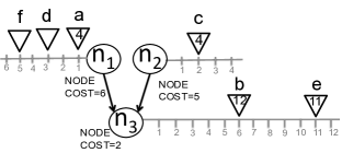
Figure 6: Three targets $n_{1},n_{2}$, and $n_{3}$ with candidate views at each target ordered by their OptCost $a$–$f$.

Example 2

Figure 6 shows a plan containing three nodes $n_{1},n_{2}$ and $n_{3}$, with node costs 6, 5, and 2 respectively, and $n_{3}$ represents $W_{n}$. Therefore, $\mbox{\sc best\-Plan}{}_{3}$ (i.e.,$\mbox{\sc best\-Plan}{}_{n}$) begins with Cost=13 (6+5+2). At each target, views ($a$–$f$) are arranged by their OptCost from their respective target nodes. For example, $b$ is placed at OptCost of 6 for node $n_{3}$. An empty triangle in the figure indicates it has not yet been considered by the algorithm; initially, all triangles begin empty. During the course of the example, if it is considered and a rewrite is found, then the actual cost of the rewrite is indicated inside.

In the first step of the rewrite algorithm, the cheapest potential rewrite for target $W_{3}$ is composed of a rewrite for $n_{1}$ using $a$ of cost 1, a rewrite for $n_{2}$ using $c$ of cost 2, and the node $n_{3}$ of cost 2, having a total OptCost of 5, whereas the next cheapest possible rewrite of $n_{3}$ uses $b$ and has an OptCost of 6. FindNextMinTarget identifies the potential rewrite composed by $a$, $c$, $n_{3}$, and it chooses $a$ as the first candidate view to Refine within this rewrite, because the OptCost of $a$ (=1) is less than $c$ (=2). After refining $a$, the actual Cost of $a$ is found to be 4, which is shown as a label inside the triangle. Note this cost is not known ahead of time, which is why the view is originally at cost of 1. Therefore $\mbox{\sc best\-Plan\-Cost}{}_{1}$ is set to 4. Now since the best known rewrite for $W_{3}$ has a total cost of 11, since $n_{1}$=4 (using a) + $n_{2}$=5 + $n_{3}$=2, then the value $\mbox{\sc best\-Plan\-Cost}{}_{3}$ is updated from 13 to 11 by PropBestRewrite.

Next it attempts the rewrite for $n_{3}$ using $b$ with an OptCost of 6, which is less than the next best choice of $(d=3)$+$(c=2)$+$(n_{3}=2)$ with a total OptCost of 7. The Cost of the rewrite of $n_{3}$ using $b$ was found to be 12 as indicated in Figure 6. Since $\mbox{\sc best\-Plan\-Cost}{}_{3}$ is already 11, it is not updated. The next best choice for $n_{3}$ is therefore the rewrite with the OptCost of 7. Within that rewrite, FindNextMinTarget chooses to refine $c$, yielding a rewrite for $n_{2}$ whose actual cost is 4, so $\mbox{\sc best\-Plan\-Cost}{}_{2}$ is set to 4. Then $\mbox{\sc best\-Plan\-Cost}_{3}$ is set to $n_{1}$=4 (using $a$) + $n_{2}$=4 (using $c$) + $n_{3}$=2, with a total cost of 10.

The algorithm proceeds to the next best possible rewrite of $(d=3)$+$(c=4)$+$(n_{3}=2)$ with OptCost of 9 which is still better than the best known rewrite of $n_{3}$ with cost of 10. The algorithm terminates when there are no possible rewrites remaining for $W_{n}$ with a OptCost less than $\mbox{\sc best\-Plan\-Cost}_{n}$. Any view with an OptCost greater than their target node’s bestPlanCost can be pruned away, e.g., $e$ at $n_{3}$ (since $11>10$) and $f$ at $n_{1}$ (since $5>4$).

It is noteworthy in Example 2 that had the algorithm started at $n_{3}$ first, it would have examined all the candidate views of $n_{3}$, resulting in a larger search space than necessary.

6.3 Proof of Correctness and Work-efficiency

The following theorem provides the proof of correctness and the work-efficiency property of our BfRewrite algorithm.

Theorem 1

BfRewrite finds the optimal rewrite $r^{*}$ of $W$ and is work-efficient.

Proof 6.2.

To ensure correctness, BfRewrite must not terminate before finding $r^{*}$. Correctness requires that we show the algorithm examines every candidate view with OptCost less than or equal to $\mbox{\sc Cost}(r^{*})$. To ensure work-efficiency, BfRewrite should not examine any extra views that cannot be included in $r^{*}$. Work-efficiency requires that we show the algorithm must not examine any candidate view with OptCost greater than $\mbox{\sc Cost}(r^{*})$. We first prove these two properties of BfRewrite for a query $W$ containing a single target, then extend these results to the case when $W$ contains $n$ targets.

For $W$ with a single target (i.e., $n=1$), proof by contradiction proceeds as follows. Consider two different rewrites $r$ and $r^{*}$ such that $r^{*}$ is the optimal rewrite and $\mbox{\sc Cost}(r^{*})<\mbox{\sc Cost}(r)$. Assume a candidate view $v^{*}$ produces the optimal rewrite $r^{*}$. Assume another candidate view $v$ produces the rewrite $r$. Suppose that BfRewrite examines $v$, sets $\mbox{\sc best\-Plan\-Cost}{}_{n}$ to $\mbox{\sc Cost}(r)$, and then terminates before examining $v^{*}$. Hence BfRewrite incorrectly reports $r$ as the optimal rewrite even though $\mbox{\sc Cost}(r^{*})<\mbox{\sc Cost}(r)$. Because BfRewrite examines candidate views by increasing OptCost, then since $v$ was examined before $v^{*}$, it must have been the case that $\mbox{\sc OptCost}(v)<\mbox{\sc OptCost}(v^{*})$. By design, BfRewrite will continue until all candidate views whose OptCost is less than or equal to $\mbox{\sc best\-Plan\-Cost}{}_{n}$ have been found. Given the lower bound property of OptCost with respect to Cost, we have that: $\mbox{\sc OptCost}(v)<\mbox{\sc OptCost}(v^{*})\leq\mbox{\sc Cost}(r^{*})<\mbox{\sc Cost}(r)=\mbox{\sc best\-Plan\-Cost}_{n}.$ From the above inequality, it is clear that the algorithm must have examined $v^{*}$ (and consequently found $r^{*}$) before terminating. This results in a contradiction since we assumed earlier that BfRewrite terminated before examining $v^{*}$.

We can similarly prove work-efficiency by contradiction as follows. Assume that $\mbox{\sc OptCost}(v)>\mbox{\sc Cost}(r^{*})$ and as above the algorithm examines $v$ before $v^{*}$. This results in the following inequality. $\mbox{\sc Cost}(r^{*})<\mbox{\sc OptCost}(v)\leq\mbox{\sc Cost}(r)=\mbox{\sc best\-Plan\-Cost}_{n}<\mbox{\sc OptCost}(v^{*}).$ The results in a contradiction since $\mbox{\sc Cost}(r^{*})$ cannot be less than $\mbox{\sc OptCost}(v^{*})$, based on the lower-bound property of OptCost.

Now we extend this result to $W$ with multiple targets, $n>1$. It is sufficient to show that the BfRewrite algorithm works by reducing $n$ individual search problems into a single global search problem that finds the optimal rewrite for the target $W_{n}$. Recall that BfRewrite instantiates a priority queue $PQ$ at each of the $n$ targets in the plan, where the candidate views at each $PQ$ are ordered by increasing OptCost. Next we show that the search process degenerates these $n$ PQs into a single virtual global $PQ$ whose elements are potential rewrites of $W_{n}$, ordered by their increasing OptCost. Recall that every invocation of FindNextMinTarget identifies the next best target to refine out of all targets in $W$. It composes the lowest cost potential rewrite for $W_{n}$ by recursively visiting each target $W_{i}$ and selecting the cheaper among either the candidate view at the front of the $PQ$ for $W_{i}$ or the current best known rewrite for $W_{i}$. Thus this recursive procedure identifies the current lowest cost potential rewrite of $W_{n}$, in effect gradually exploring the space of potential rewrites of $W_{n}$ by their increasing OptCost. This creates a virtual global $PQ$ whose elements are potential rewrites of $W_{n}$ and is ordered by their OptCost.

For example, in Figure 6, note that the first potential rewrite for $W_{n}$ is composed of $a,c,n_{3}$ with an OptCost of 5, while the next potential rewrite of $W_{n}$ is composed of $b$ with an OptCost of 6. Furthermore, notice that the rewrite produced by $a,c,n_{3}$ has a cost of 10, which is always greater than or equal to its corresponding OptCost due to the lower-bound property. We have now reduced $n$ priority queues of candidate views ordered by OptCost to a single global priority queue of potential rewrites of $W_{n}$ ordered by OptCost. This completes the proof since we already showed above that BfRewrite with a single $PQ$ ordered by OptCost will find the optimal rewrite and is work-efficient.

7 ViewFinder

The key feature of ViewFinder is its OptCost functionality that enables it to incrementally explore the the space of rewrites using the views in $V$. As noted earlier in Section 4.1, rewriting queries using views is known to be a hard problem. Traditionally, methods for rewriting queries using views for SPJG queries use a two stage approach [8, 2]. The pruning stage determines which views are relevant to the query, and among the relevant views those that contain all the required join predicates are termed as complete, otherwise they are called partial solutions. This is typically followed by a merge stage that joins the partial solutions using all possible equijoin methods on all join orders to form additional relevant views. The algorithm repeats until only those views that are useful for answering the query remain.

We take a similar approach in that we identify partial and complete solutions, then follow with a merge phase. The ViewFinder considers candidate views $C$ when searching for rewrite of a target. $C$ includes views in $V$ as well as views formed by “merging” views in $V$ using a Merge function, which is an implementation of a standard view-merging procedure (e.g., [2, 8]). Traditional approaches merge partial solutions to create complete solutions, continuing until no partial solutions remain. This “explodes” the space of candidate views exponentially up-front. In contrast, our approach gradually explodes the space, resulting in far fewer candidates views from being considered.

Additionally, with no early termination condition, existing approaches would need to explore the space exhaustively at all targets. The ViewFinder incrementally grows and explores only as much of the space as needed, frequently stopping and resuming the search as requested by BfRewrite.

7.1 The ViewFinder Algorithm

The ViewFinder is presented in Algorithm 4. There is an instance of ViewFinder instantiated at each target, which is stateful; enabling it to start, stop, and resume the incremental searches at each target. The ViewFinder maintains state using a priority queue (PQ) of candidate views, ordered by OptCost. ViewFinder implements the Init, Peek, and Refine functions.

The Init function instantiates an instance of the ViewFinder with a query $q$ representing a target $W_{i}$, and the set of all materialized views $V$ is added to PQ.

The Peek function is used by BfRewrite to obtain the OptCost of the head item in a PQ.

The Refine function is invoked when BfRewrite asks the ViewFinder to examine the next candidate view. At this stage, the ViewFinder pops the head item $v$ out of PQ. The ViewFinder then generates a set of new candidate views $M$ by merging $v$ with previously popped candidate views (i.e., views in $Seen$), thereby incrementally exploding the space of candidate views. Note that $Seen$ only contains candidate views that have an OptCost less than or equal to that of $v$. Merged views in $M$ are only retained if they are not already in $Seen$. Then views in $M$ are inserted into PQ and $v$ is added to $Seen$.

A property of OptCost (provided as a theorem below) is that the candidate views in $M$ have an OptCost that is greater than that of $v$ and hence none of these views should have been examined before $v$. Critically, this enables ViewFinder to perform a gradual explosion of the space of candidate views. At this point, the view is considered for a rewrite as described next.

Theorem 7.3.

The OptCost of every candidate view in $M$ that is not in $Seen$ is greater than or equal to the OptCost of $v$.

Proof 7.4.

The proof sketch is as follows. The theorem is trivially true for $v\in V$ as all candidate views in $M$ cannot be in $Seen$ and have OptCost greater than $v$. If $v\notin V$, it is sufficient to point out that all constituent views of $v$ are already in $Seen$ since they must have had OptCost lesser or equal to $v$ Hence all candidate views in $M$ with OptCost smaller than $v$ are already in $Seen$, and those with OptCost greater than $v$ will be added to $PQ$ if they are not already in $PQ$.

Algorithm 4 ViewFinder

1:function Init($query$, $V$)

2:   Priority Queue $PQ$ $\leftarrow$$\emptyset$; $Seen$ $\leftarrow$$\emptyset$; Query $q$

3:   $q$ $\leftarrow$$query$

4:   for each $v\in V$ do

5:     $PQ$.add($v$, $\mbox{\sc OptCost}(q,v))$

6:   end for

7:end function

1:function Peek

2:   if $PQ$ is not empty return $PQ$.peek().OptCost else $\infty$

3:end function

1:function Refine

2:   if not $PQ$.empty() then

3:     $v$ $\leftarrow$$PQ$.pop()

4:     $M$ $\leftarrow$Merge($v$, $Seen$) $\triangleright$ Discard from $M$ those in $Seen\cap M$

5:     for each $v^{\prime}\in M$ do

6:        $PQ$.add($v^{\prime}$, $\mbox{\sc OptCost}(q,v^{\prime})$)

7:     end for

8:     $Seen$.add($v$)

9:     if GuessComplete($q$, $v$) then

10:        return $\mbox{\sc Rewrite\-Enum}(q,v)$

11:     end if

12:   end if

13:return null

14:end function

7.2 Rewrite Enumeration

Given the computational cost of finding valid rewrites, BfRewrite limits the invocation of the RewriteEnum algorithm using two strategies. First, we avoid having to apply RewriteEnum on every candidate view by using GuessComplete. Second, we delay the application of RewriteEnum to every complete view by determining a lower bound on the cost of a rewrite by using OptCost.

The RewriteEnum procedure (pseudo-code not shown but described here) searches for a valid rewrite of a query $q$ using a view $v$ that is guessed to be complete. Given that GuessComplete can result in false positives, a rewrite may not be found. If a rewrite is found, RewriteEnum returns the rewrite and its cost as determined by the Cost function.

From Section 5, recall that the rewrite process only considers a subset of the UDFs in the system and standard relational operators SPJGA. These are the only transformations considered by RewriteEnum. The rewrite process searches for equivalent rewrites of $q$ by applying compensations [23] to a view $v$ that is guessed to be complete for $q$, using only the transformations. RewriteEnum does this by generating all permutations of required compensations and testing for equivalence, which amounts to a brute force enumeration of all possible rewrites that can be produced by applying the transformations. This makes the case for the system to keep the set of transformations small since this search process is exponential in the size of this set. When the transformations are restricted to a fixed known set, it may suffice to examine a polynomial number of rewrites attempts, as in [7] for the specific case of simple aggregations involving group-bys. Such approaches are not applicable to our case as the system has the flexibility to add any UDF to the set of transformations.

8 Experimental Evaluation

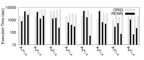
(a)                                                                                                                                                               (b)

Figure 7: Query evolution comparisons for (a) execution time (log-scale), and (b) execution time improvement.

In this section, we present an experimental study we conducted in order to validate the effectiveness of BfRewrite in finding low-cost rewrites of complex queries. We first evaluate our methods in two scenarios. The query evolution scenario (Section 8.3.1) represents a user iteratively refining a query within a single session. This scenario evaluates the benefit that each new query version can receive from the opportunistic views created by previous versions of the query. The user evolution scenario (Section 8.3.2) represents a new user entering the system presenting a new query. This scenario evaluates the benefit a new query can receive from the opportunistic views created by queries of other “similar” users. We compare the performance of our algorithm with a competing approach in (Section 8.3.3). Next, we evaluate the scalability (Section 8.3.3) of our rewrite algorithm in comparison to the dynamic programming approach. We then compare our method to cache-based methods (Section 8.3.4) that can only reuse identical previous results. Lastly, we show the performance of our method (Section 8.3.5) under a storage reclamation policy that drops opportunistic views.

8.1 Methodology

Our experimental system consists of 20 machines running Hadoop. We use HiveQL as the declarative query language, and Oozie as a job coordinator. The MR UDFs are implemented in Java, Perl, and Python and executed using the HiveCLI. UDFs implemented in our system include a log parser/extractor, text sentiment classifier, sentence tokenizer, lat/lon extractor, word count, restaurant menu similarity, and geographical tiling, among others. All UDFs are annotated using the model, as per the example annotations given in Section 3.2.

Our experiments use the following three real-world datasets totalling over 1TB: a Twitter log containing 800GB of tweets, a Foursquare log containing 250GB of user check-ins, and a Landmark log containing 7GB of 5 million landmarks including their locations. The identity of a social network user (user_id) is common across Twitter and Foursquare logs, while the identity of a landmark (location_id) is common across Foursquare and Landmarks logs.

For all experiments, we report on the following metrics. Experiments on query execution time report both the original execution time of the query in Hive, labelled as orig, and the execution time of the rewritten query, labelled as rewr. The reported time for rewr includes the time to run the BfRewrite algorithm, the time to execute the rewritten query, and any time spent on statistics collection (Section 2). Experiments on rewrite algorithm runtime report the total optimization time used by the algorithm to find a rewrite of the original query using the views in the system. For these experiments, bfr denotes the use of our BfRewrite algorithm, and dp represents a competing rewrite approach. dp does not use OptCost and searches exhaustively for rewrites at every target, then applies a dynamic programming solution to choose the best subset of rewrites found at each target to rewrite the query. It is to be noted that both algorithms produce identical rewrites (i.e., $r^{*}$). The primary comparison metric for bfr and dp is the algorithm runtime, and secondary metrics are the number of candidate views examined during the search for rewrites, and the number of valid rewrites produced, i.e., the space explored and rewrites attempted before $r^{*}$ is found.

8.2 Query Workload

The experimental workload contains 32 queries simulating 8 analysts $A_{1}$–$A_{8}$ who write complex analytical queries for business marketing scenarios from [14]. These queries represent exploratory analysis on big data, and contain UDFs. Each analyst in the workload poses 4 versions of a query, representing the initial query followed by three subsequent revisions made during data exploration and hypothesis testing. Hence, there is some overlap expected between subsequent version of a query. The queries are long-running with many operations, and executing the original versions of the queries in Hive created 17 opportunistic materialized views on average.

As each query has multiple versions, we use $A_{i}v_{j}$ to denote Analyst $i$ executing version $j$ of her query, and version $j$ represents a revised version of $j-1$. We briefly describe the first two versions of $A_{1}$’s query in Example 8.5. The queries reference data from Twitter (TWTR), Foursquare (4SQ), and Landmarks (LAND) data, and UDFs are denoted in all caps.

Example 8.5.

Analyst1 ($A_{1}$) wants to identify a number of “wine lovers” to send them a coupon for a new wine being introduced in a local region.

Query $A_{1}v_{1}$: (a) From TWTR, apply UDF-CLASSIFY-WINE-SCORE on each user’s tweets and group-by user to produce wine-sentiment-score for each user. Apply a threshold on wine-sentiment-score. (b) From TWTR, compute all pairs $\langle u_{1},u_{2}\rangle$ of users that communicate with each other, assigning each pair a friendship-strength-score based on the number of times they communicate. Apply a threshold on friendship-strength-score. (c) From TWTR, apply UDAF-CLASSIFY-AFFLUENT on users and their tweets. Join results from (a), (b), (c) on user_id.

Query $A_{1}v_{2}$: Revise the previous version by reducing the wine-sentiment-score threshold, adding new data sources (4SQ and LAND) to find the check-in counts for users that check-in to places of type wine-bar, then threshold on count and join with users found in the previous version. Query Versions 3 and 4 are revised similarly but omitted here.

8.3 Experimental Results

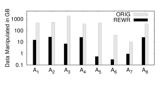
(a)                                                                                                      (b)                                                                                                      (c)

Figure 8: User Evolution Comparisons for (a) execution time (log-scale), (b) data moved, and (c) execution time improvement.

8.3.1 Query Evolution

In this experiment, for each analyst $A_{i}$, query $A_{i}v_{1}$ is executed, followed by query $A_{i}v_{2}$, $A_{i}v_{3}$, and $A_{i}v_{4}$. Figure 7(a) shows the execution time of the original query (orig) and the rewritten query (rewr), and Figure 7(b) reports the percent improvement in execution time of rewr over orig. Figure 7(b) shows rewr provides an overall improvement of 10% to 90%; with an average improvement of 61% and up to an order of magnitude. As a concrete data point, $A_{5}v_{4}$ requires 54 minutes to execute orig, but only 55 seconds to execute the rewritten query (rewr). rewr has much lower execution time because it is able to take advantage of the overlapping nature of the queries, e.g., version 2 has some overlap with version 1. rewr is able to reuse previous results, which provides a significant savings in computation time and data movement (read/write/shuffle) costs.

8.3.2 User Evolution

In this experiment, we first execute the first version of each analyst’s query except one (holdout analyst $A_{i}$). Then, we execute the first version of the holdout analyst’s query ($A_{i}v_{1}$), and repeat this with a different holdout analyst each time. Figure 8(a) shows the execution time for rewr and orig for each different holdout analyst along the x-axis, while Figure 8(b) shows the corresponding data manipulated (read/write/shuffle) in GB. These results demonstrate that the execution time is always lower for rewr, with the amount of data moved showing a similar trend. The percentage improvement in execution time is given in Figure 8(c) which shows rewr results in an overall improvement of about 50%–90%. This scenario mimics a new analyst arriving in a system, and the results show the benefit that is obtained by reusing previous results from many other analysts that pose queries on the same data. Of course, these results are workload dependent but they show that even when analysts query the same data sets while testing different hypothesis, our approach is able to find some overlap and benefit from previous results.

Table 1: Improvement in execution time of $A_{5}v_{3}$ as more analysts become present in the system.

Analysts added	1	2	3	4	5	6	7
Improvement	0%	73%	73%	75%	89%	89%	89%

As an additional experiment for user evolution, we first execute a single analyst’s query ($A_{5}v_{3}$) with no opportunistic views in the system, to create a baseline execution time. Then we “add” another analyst by executing all four versions of that analyst’s query, which creates new opportunistic views. Then we re-execute $A_{5}v_{3}$ and report the execution time improvement over the baseline, and repeat this process for the other remaining analysts. We chose $A_{5}v_{3}$ as it is a complex query that uses all three logs. Table 1 reports the execution time improvement after each analyst is added, showing that the improvement increases when more opportunistic views are present in the system.

8.3.3 Algorithm Comparisons

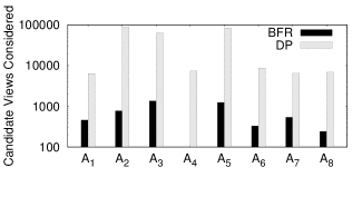
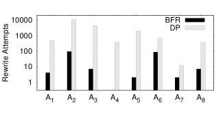
(a)                                                                                                      (b)                                                                                                      (c)

Figure 9: Algorithm Comparisons for (a) candidate views considered, (b) refine attempts, and (c) Algorithm runtime (log-scale).

In the first experiment we compare bfr to dp in terms of the number of candidate views considered, the number of times the algorithm attempts a rewrite, and the algorithm runtime in seconds. We use the user evolution scenario from the previous experiment, where there were approximately 100 views in the system when each holdout analyst’s query was executed. Figure 9(a) shows that even though both algorithms find identical rewrites, bfr searches much less of the space than dp since it considers far fewer candidate views when searching for rewrites. Similarly, Figure 9(b) shows that bfr attempts far fewer rewrites compared to dp. This improvement can be attributed to GuessComplete identifying the promising candidate views, and OptCost enabling bfr to incrementally explore the candidate views, thus applying RewriteEnum far fewer times. Together, these contribute to bfr doing far less work than dp, which is reflected in the algorithm runtime shown in Figure 9(c). This shows our algorithm results in significant savings due to the way it controls the exponential burst of candidate views, growing the candidates set incrementally as needed, and by controlling the number of times it attempts a rewrites; all of which are all computationally expensive since they are exponential in either the number of candidate views or the number of transformations. Next we show how bfr scales as the number of views increases.

Figure 10: Runtime of bfr and dp for varying number of MVs.

In the second experiment, we test the scalability of the algorithms by scaling up the number of views in the system from 1–1000 and report the algorithm runtime for both bfr and dp as they search for rewrites for one query ($A_{3}v_{1}$). During the course of design and development of our system, we created and retained about 9,600 views; from these we discarded duplicate views as well as those views that are an exact match to the query (simply to prevent the algorithms from terminating trivially). In Figure 10, the x-axis reports the the number of views (views are randomly drawn from among these candidates), while the y-axis reports the algorithm run time (log-scale). dp becomes prohibitively expensive even when 250 MVs are present in the system, due to the exponential search space. bfr on the other hand scales much better than dpr and has a runtime under 1000 seconds even when the system has 1000 views relevant to the given query. This is due to the ability of bfr to control the exponential space explosion and incrementally search the rewrite space in a principled manner.

While this runtime is not trivial, we note that these are complex queries involving UDFs that run for thousands of seconds. The amount of time spent to rewrite a query plus the execution time of the rewritten query is far less than the execution time of the original query. For instance, Figure 8(a) reports a query execution time of 451 seconds for $A_{5}$ optimized versus 2134 seconds for unoptimized. Even if the rewrite time for $A_{5}$ were 1000 seconds (it is actually 3.1 seconds here as seen in Figure 9(c)), the total execution time would still be 32% faster than the original query.

8.3.4 Comparison with Caching-based methods

Next we provide a brief comparison of our approach with caching-based methods (such as [5]) that perform only syntactic matching when reusing previous results. With this class of solutions, results can only be reused to answer a new query when their respective execution plans are identical, i.e., the query plan and the plan that produced the previous results must be syntactically identical. This means that if the respective plans differ in any way (e.g., different join orders or predicate push-downs), then reuse is not possible. For instance, with syntactic matching, a query that applies two filters in sequence $a,b$ will not match a view (i.e., a previous result) that has applied the same two filters in a different sequence $b,a$. In contrast, our bfr approach performs semantic matching and query rewriting. In this case, not only will bfr match $a,b$ with $b,a$, but it would also match the query to a view that only has $b$, by applying an additional filter $a$ during the rewrite process.

To represent the class of syntactic caching methods, we present a conservative variant of our approach that performs a rewrite only if a view and a query have identical $A,F,K$ properties as well as have identical plans. We term this variant bfr-syntactic.

Figure 11 highlights the limitations of caching-based methods by repeating the query evolution experiment for Analyst 1 ($A_{1}v_{1}$–$A_{1}v_{4}$). We first execute query $A_{1}v_{1}$ to produce opportunistic views, and then we apply both bfr and bfr-syntactic to queries $A_{1}v_{2}$, $A_{1}v_{3}$ and $A_{1}v_{4}$ and report the results in terms of query execution time improvement of the solutions produced by bfr and bfr-syntactic. Figure 11 shows that both bfr and bfr-syntactic result in the same execution time improvement for $A_{1}v_{2}$. This is because both methods were able to reuse some of the (syntactically identical) views from the previous query. However, bfr-syntactic performs worse than bfr for query $A_{1}v_{3}$ and $A_{1}v_{4}$. This is because bfr-syntactic was unable to find many views that were exact syntactic matches, whereas bfr was able to exploit additional views due to bfr’s ability to reuse and re-purpose previous results through semantic query rewriting. Even though this particular result is workload dependent, this example highlights the fact that while reusing identical results is clearly beneficial, our approach completely subsumes those that only reuse syntactically identical results: even when there are no identical views our method may still produce a low-cost rewrite.

As an additional point of comparison with caching-based methods, we next perform an experiment in which we remove all identical views from the system and then apply our bfr algorithm.

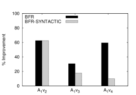
Figure 11: Execution time improvement for bfr and bfr-syntactic.

Table 2: Execution time improvement without identical views.

Analyst	$A_{1}$	$A_{2}$	$A_{3}$	$A_{4}$	$A_{5}$	$A_{6}$	$A_{7}$	$A_{8}$
BfRewrite	57%	64%	83%	85%	51%	96%	88%	84%

Here we repeat the user evolution experiment after discarding from the system all views that are identical to a target in each of the holdout queries ($A_{1-8}v_{1}$). Without these views, syntactic caching-based methods will not be able to find any rewrites, resulting in 0% improvement. Table 2 reports the percentage improvement for each analyst $A_{1}$–$A_{8}$ after discarding all identical views. This shows bfr continues to reduce query execution time dramatically even when there are no views in the system that are an exact match to the new queries. The performance improvements are comparable to the result in Figure 8(c) which represents the same experiment without discarding the identical views. Notably there is a drop for $A_{5}$ compared to the results reported in Figure 8(c) for $A_{5}$. This is because previously in Figure 8(c), $A_{5}$ had benefited from an identical view corresponding to a restaurant-similarity computation that it now has to recompute. The identical views discarded constituted only 7% of the view storage space in this experiment, indicating there are many other useful views. Given that analysts pose different but related queries in an evolutionary analytical scenario, any method that relies solely on identical matching may have limited benefit.

8.3.5 Storage Reclamation

Table 3: Execution Time Improvement after reclaiming 10% to 90% of the view storage space.

View Storage Space	$2.0\times$	$1.8\times$	$1.5\times$	$1.0\times$	$0.6\times$	$0.2\times$
Improvement	89%	89%	86%	82%	58%	30%

Since storage is not infinite, a reclamation policy is necessary. Although choosing a beneficial set of views to retain within a finite storage budget is an interesting problem for future work, here we apply two simple policies for storage reclamation. Our aim in this experiment is to show the robustness of our approach even when the reclamation policy makes unsophisticated choices such as dropping views randomly or dropping all of the views identical to a given query.

First, we repeat the experiment in Section 8.3.2 using the $A_{5}v_{3}$ query, but reduce the view storage budget each time. Retaining all views resulted in a storage space of approximately $2.0\times$ the base data size ($\approx$2TB). The relatively small total size of the views with respect to the log base data is due to several reasons. First, the logs are very wide, as they record a large number of attributes. However, a typical query only consumes a small fraction of these log attributes, which consistent with observations in big data systems. Second, it is not uncommon for the log attributes to have missing values, since the data may be dirty or incomplete. For instance, in the Twitter log, a tweet may have missing location values. Thus a query may discard those tweets without location values. Third, in this experiment, views are not duplicated since the rewriter makes use of existing views whenever possible. For these reasons, the total size of the views is relatively small compared to the size of the base data.

Table 3 reports the execution time improvement for the rewritten query compared to the original query for each storage budget. We repeat each experiment twice, each time randomly dropping views from the full set of views, and report the average improvement. The results show that our method is able to find good rewrites using the remaining views available, until the view storage budget is very small. Second, by the results shown earlier in Table 2, our method is able to find good rewrites even when there are no identical views in the system; which could be the case if a poor reclamation policy were used. Designing a good storage reclamation policy is equivalent to the view selection problem [17] with a storage constraint.

9 Related Work

Query Rewriting Using Views. There is a rich body of previous work on rewriting queries using views, but these only consider a restricted class of queries. Representative work includes the popular algorithm MiniCon [20], recent work [13, 12] showing how rewriting can be scaled to a large number of views, and rewriting methods implemented in commercial databases [6, 23]. However, in these works both the queries and views are restricted to the class of conjunctive queries (SPJ) or additionally include groupby and aggregation (SPJGA).

Our work differs in the following two ways: (a) We show how UDFs can be included in the rewrite process using our UDF model, which results in a unique variant of the rewrite problem when there is a divergence between the expressivity of the queries and that of the rewrite process; (b) Our rewrite search process is cost-based—OptCost enables the enumeration of candidate views based on their ability to produce a low-cost rewrite. In contrast, traditional approaches (e.g., [6, 20]) typically determine containment first (i.e., if a view can answer a query) and then apply cost-based pruning in a heuristic way. This unique combination of features has not been addressed in the literature for the rewrite problem.

Online Physical Design Tuning. Methods such as [21] adapt the physical configuration to benefit a dynamically changing workload by actively creating or dropping indexes/views. Our work is opportunistic, and simply relies on the by-products of query execution that are almost free. However, view selection methods could be applicable during storage reclamation to retain only those views that provide maximum benefit.

Reusing Computations in MapReduce. Other methods for optimizing MapReduce jobs have been introduced such as those that support incremental computations [16], sharing computation or scans [18], and re-using previous results [5]. As shown in Section 8.3.4, our approach completely subsumes these methods.

Multi-query optimization (MQO). The goal of MQO [22] (and similar approaches [18]) is to maximize resource sharing, in particular common intermediate data, by producing a scheduling strategy for a set of in-flight queries. Our work produces a low-cost rewrite rather than a schedule for concurrent query plans.

10 Conclusion

Big data analytics is characterized by exploratory queries with frequent use of UDFs containing arbitrary user code. To exploit previous results effectively, some understanding of UDFs is required. In this work, we presented a gray-box UDF model that is simple but expressive enough to capture a large class of big data UDFs, enabling our system to exploit prior computation.

However, considering many UDFs can make the space of rewrites impractical since any UDF in the system may be included in the rewrite process. We presented a rewrite algorithm BfRewrite that utilizes a lower-bound on the cost of a potential rewrite in order to incrementally grow and search the space of rewrites. Furthermore, we prove BfRewrite is work-efficient and finds the optimal rewrite. Our experiments show that for a workload of queries that make extensive use of UDFs, our method results in dramatic performance improvements with an average of 61% and up to an order of magnitude.

References

- [1] S. Abiteboul and O. M. Duschka. Complexity of answering queries using materialized views. In PODS, 1998.
- [2] S. Agrawal, S. Chaudhuri, and V. Narasayya. Automated selection of materialized views and indexes in SQL databases. In VLDB, 2000.
- [3] Anonymous PDF document. https://drive.google.com/file/d/0Bzw_KGVFEyOpMFlmUzJEaHB5NkU.
- [4] DataFu. http://data.linkedin.com/opensource/datafu.
- [5] I. Elghandour and A. Aboulnaga. ReStore: reusing results of MapReduce jobs. PVLDB, 5(6), 2012.
- [6] J. Goldstein and P.-A. Larson. Optimizing queries using materialized views: A practical, scalable solution. In SIGMOD, 2001.
- [7] S. Grumbach and L. Tininini. On the content of materialized aggregate views. In PODS, 2000.
- [8] A. Halevy. Answering queries using views: A survey. VLDBJ, 10(4), 2001.
- [9] G. Hjaltason and H. Samet. Index-driven similarity search in metric spaces. TODS, 28(4), 2003.
- [10] F. Hueske, M. Peters, M. J. Sax, A. Rheinländer, R. Bergmann, A. Krettek, and K. Tzoumas. Opening the black boxes in data flow optimization. PVLDB, 5(11), 2012.
- [11] T. S. Jayram, P. G. Kolaitis, and E. Vee. The containment problem for Real conjunctive queries with inequalities. In PODS, 2006.
- [12] G. Konstantinidis and J. Ambite. Optimizing query rewriting for multiple queries. In IIWeb, 2012.
- [13] G. Konstantinidis and J. L. Ambite. Scalable query rewriting: a graph-based approach. In SIGMOD, 2011.
- [14] J. LeFevre, J. Sankaranarayanan, H. Hacıgümüş, J. Tatemura, and N. Polyzotis. Towards a workload for evolutionary analytics. In SIGMOD Workshop on Data Analytics in the Cloud (DanaC), 2013.
- [15] A. Y. Levy, A. O. Mendelzon, and Y. Sagiv. Answering queries using views (extended abstract). In PODS, 1995.
- [16] B. Li, E. Mazur, Y. Diao, A. McGregor, and P. Shenoy. A platform for scalable one-pass analytics using MapReduce. In SIGMOD, 2011.
- [17] I. Mami and Z. Bellahsene. A survey of view selection methods. SIGMOD Rec., 41(1), 2012.
- [18] T. Nykiel, M. Potamias, C. Mishra, G. Kollios, and N. Koudas. MRShare: sharing across multiple queries in MapReduce. VLDB, 3(1-2), 2010.
- [19] PiggyBank. https://cwiki.apache.org/confluence/display/PIG/PiggyBank.
- [20] R. Pottinger and A. Halevy. MiniCon: A scalable algorithm for answering queries using views. VLDB, 10(2), 2001.
- [21] K. Schnaitter, S. Abiteboul, T. Milo, and N. Polyzotis. On-line index selection for shifting workloads. In ICDE, 2007.
- [22] T. Sellis. Multiple-query optimization. TODS, 13(1), 1988.
- [23] M. Zaharioudakis, R. Cochrane, G. Lapis, H. Pirahesh, and M. Urata. Answering complex SQL queries using automatic summary tables. In SIGMOD, 2000.