Dynamics of X-Ray–Emitting Ejecta in the Oxygen-Rich Supernova Remnant Puppis A Revealed by the XMM-Newton RGS

Abstract

Using the unprecedented spectral resolution of the reflection grating spectrometer (RGS) onboard XMM-Newton, we reveal dynamics of X-ray–emitting ejecta in the oxygen-rich supernova remnant Puppis A. The RGS spectrum shows prominent K-shell lines, including O VII He$\alpha$ forbidden and resonance, O VIII Ly$\alpha$, O VIII Ly$\beta$, and Ne IX He$\alpha$ resonance, from an ejecta knot positionally coincident with an optical oxygen-rich filament (the so-called “$\Omega$” filament) in the northeast of the remnant. We find that the line centroids are blueshifted by 1480$\pm$140$\pm$60$\>\rm{\,km\,s}^{-1}$ (the first and second term errors are measurement and calibration uncertainties, respectively), which is fully consistent with that of the optical $\Omega$ filament. Line broadening at 654 eV (corresponding to O VIII Ly$\alpha$) is obtained to be $\sigma\lesssim 0.9$ eV, indicating an oxygen temperature of $\lesssim 30$ keV. Analysis of XMM-Newton MOS spectra shows an electron temperature of $\sim$0.8 keV and an ionization timescale of $\sim$2$\times$10¹⁰ $\rm{\,cm}^{-3}\,$s. We show that the oxygen and electron temperatures as well as the ionization timescale can be reconciled if the ejecta knot was heated by a collisionless shock whose velocity is $\sim$600–1200$\>\rm{\,km\,s}^{-1}$ and was subsequently equilibrated due to Coulomb interactions. The RGS spectrum also shows relatively weak K-shell lines of another ejecta feature located near the northeastern edge of the remnant, from which we measure redward Doppler velocities of 650$\pm$70$\pm$60$\>\rm{\,km\,s}^{-1}$.

1 Introduction

The Galactic supernova remnant (SNR) Puppis A is one of the so-called “oxygen-rich” SNRs, in which oxygen-rich fast-moving optically emitting ejecta knots (OFMKs) are identified. So far, eight other SNRs, Cas A and G292.0+1.8 in our Galaxy and six others in the Magellanic Clouds and NGC 4449, are categorized in this class (Vink, 2012, for a recent summary). Of these, Puppis A is particularly interesting, because all of OFMKs are located in the eastern and northeastern (NE) portion (Winkler & Kirshner, 1985; Winkler et al., 1988), while the stellar remnant is moving in the opposite southwestern direction (Petre et al., 1996; Hui & Becker, 2006; Winkler & Petre, 2007; Becker et al., 2012). This is consistent with recent models, which predicts that SN ejecta are expelled preferentially in one direction, while the stellar remnant receives a kick in the opposite direction (Wongwathanarat et al., 2012, and references therein). Thus, Puppis A is an extremely important target for the study of SN explosion mechanisms as well as SN nucleosynthesis.

Puppis A is one of the brightest SNRs in the X-ray sky. The X-ray emission has been thought to be dominated by strong cloud-shock interactions (Charles et al., 1978; Petre et al., 1982, references therein). A large area of the remnant was recently mapped by X-ray observatories in orbit, i.e., XMM-Newton, Chandra, and Suzaku. They confirmed earlier results that the X-ray emission is dominated by the swept-up interstellar medium (Hwang et al., 2005, 2008; Katsuda et al., 2010). On the other hand, the data also revealed signatures of SN ejecta in three locations: a Si-rich clump (Hwang et al., 2008), a bright O-Ne-Mg-(Si-S)-rich knot (the ejecta knot called hereafter: Katsuda et al., 2008), whose southern portion is positionally coincident with an “$\Omega$”-shaped OFMK (the so-called $\Omega$ filament named by Winkler & Kirshner, 1985), and an O-Ne-Mg-rich filament (the ejecta filament called hereafter: Katsuda et al., 2010). All of them are located in the NE quadrant, further supporting the one-sided ejection of SN debris.

While picking up ejecta features reveal two dimensional ejecta distributions on the plane of the sky, measurements of Doppler velocities can provide us with line-of-sight structures (Dewey, et al., 2010, for a recent review of kinematics of X-ray SNRs). Katsuda et al. (2008) found that the ejecta knot described above shows blueshifted K-shell lines. The Doppler velocities were measured to be 3400${}^{+1000}_{-800}$$\>\rm{\,km\,s}^{-1}$ at the northern knot and 1700${}^{+700}_{-800}$$\>\rm{\,km\,s}^{-1}$ at the southern knot which agrees with the optical measurement of $\sim$1500$\>\rm{\,km\,s}^{-1}$ (Winkler & Kirshner, 1985). The possible different Doppler velocities between the north and the south led us to suggest that the ejecta knot actually consists of two different knots which appear to be located close with each other. However, the poor quality of the data prevented us from making strong arguments; the X-ray data were taken by the XMM-Newton European Photon Imaging Camera (EPIC: Turner et al., 2001; Strüder et al., 2001) with moderate spectral resolution ($E/\Delta E\sim 20$), and also the ejecta knot was detected at the edge of the field of view (FOV) where calibration uncertainties would be large.

Here, we report on precise Doppler measurements for the ejecta knot and the ejecta filament in Puppis A, based on the unprecedented spectral resolution X-ray spectra ($E/\Delta E\sim 150$) obtained by the Reflection Grating Spectrometer (RGS: den Herder et al., 2001) onboard XMM-Newton. In addition, we give a restrictive upper limit on an oxygen temperature of the ejecta knot, for the first time. These new measurements allow us to discuss the nature of the ejecta knot in detail.

2 Observation and Data Reduction

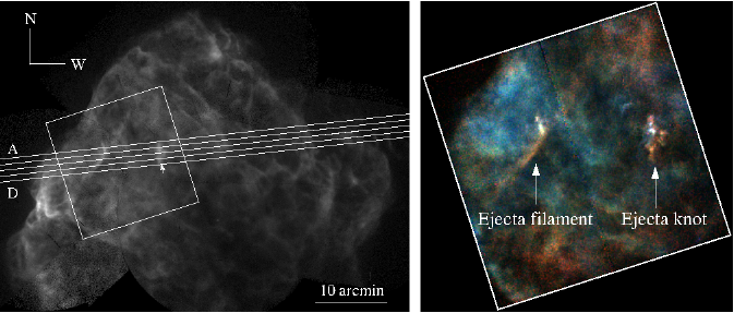
Figure 1: Left: The RGS spectral extraction regions overlaid on the merged XMM-Newton and Chandra image in the energy band 0.5–5 keV. The arrow indicates zero points of projection profiles shown in Figure 2. Right: Three-color close-up Chandra image of the white box region in the left panel. Red, green, and blue correspond to 0.5–0.7 keV, 0.7–1.2 keV, and 1.2–5.0 keV, respectively. Two ejecta features focused in this paper are indicated as arrows.

We performed an XMM-Newton observation of Puppis A on 2012 October 20 (Obs.ID 0690700201), aiming at the fast-moving ejecta knot coincident with the optical $\Omega$ filament. Our primary instrument in this observation is the RGS that can produce high-resolution X-ray spectra, while we also make use of the EPIC data to support the RGS results as well as to obtain additional information. The dispersion direction of the RGS is 96^∘.4 measured east to north, as we show in Figure 1 left—an X-ray image of Puppis A generated by existing XMM-Newton and Chandra data. Fortunately, no background flare is seen in our light curve, allowing us to use full exposure times of 20.8 ks, 12.1 ks, and 11.7 ks for the RGS1/2, MOS1, and MOS2, respectively. All the raw data were processed using version 11.0.0 of the XMM Science Analysis Software and the calibration data files available in 2012 May.

3 RGS Spectra

The slitless RGS spectrometer is generally not useful for extended sources like Puppis A, because off-axis emission along the dispersion direction is detected at wavelength positions shifted with respect to the on-axis source, which causes degradation of energy resolution. However, if the angular size of the target is small enough ($\lesssim$ a few arc minutes) and is brighter than its surroundings, it is possible to obtain high-resolution spectra for them. Our on-axis source, the ejecta knot, is such a lucky case, for which we are able to obtain an order-of-magnitude better resolution spectra than nondispersive CCDs. There is another ejecta feature, i.e., the ejecta filament described in the introduction, within the RGS FOV. Since the angular size of the filament along the dispersion direction is as thin as 1^′, we can also find its signatures in the RGS spectrum. The two ejecta features of interest are indicated on a Chandra image shown in Figure 1 right.

The analysis method basically follows our previous work (Katsuda et al., 2012). Briefly, we first extract four RGS spectra from 0^′.8-width sectors along the cross-dispersion direction. We then smooth the RGS response designed for on-axis point sources, based on emission profiles along the dispersion direction by using the rgsrmfsmooth software. Finally, we fit the RGS spectrum with emission models in the XSPEC package (Arnaud, 1996). The RGS background (BG) is generated from a blank-sky observation (Lockman hole: Obs.ID 0147511601), as we did in our previous work. The blank-sky BG emission is less than 1% of the source emission in the energy band analyzed.

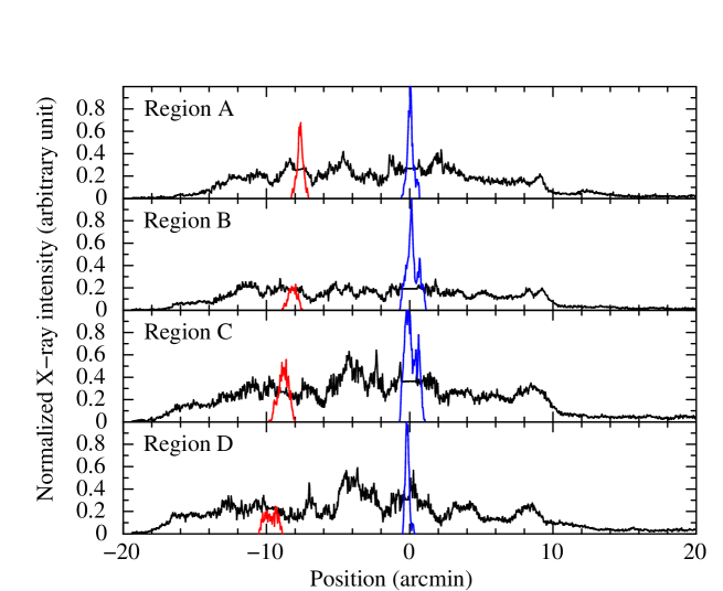
Figure 2: X-ray emission profiles in 0.6–0.7 keV along the RGS dispersion axis for the four spectral extraction regions. The three profiles in each panel are responsible for the ejecta knot in blue, the ejecta filament in red, and the diffuse surroundings in black. The X-ray intensities are normalized at the peak values of the ejecta knot, showing how diffuse surrounding emission is significant in the RGS spectra. The zero points in x-axis (x=0) correspond to the direction from which emission is detected at the nominal (no red/blue shift) wavelength positions on the RGS detectors.

Here, the RGS response in each region is smoothed with three distinct emission profiles responsible for (1) the ejecta knot, (2) the ejecta filament, and (3) their surrounding diffuse emission, so that we can derive physical parameters for individual features. Emission profiles are generated with either the Chandra or XMM-Newton image, for which we take account of vignetting effects of XMM-Newton’s X-ray telescope and the asymmetry of the effective area along the dispersion axis described in the literature (Broersen et al., 2013). The emission profiles for the ejecta features are extracted from Chandra images masked for them, for which we subtract underlying diffuse emission by interpolating the surrounding diffuse emission. We have checked that, even if we change the intensity of underlying diffuse emission by $\pm$20% which is a small-scale inhomogeneity around the ejecta knot, the fit results presented below are not affected significantly. Figure 2 shows the X-ray emission profiles in 0.6–0.7 keV for the four regions. The three profiles in each panel are responsible for (1) the ejecta knot in blue, (2) the ejecta filament in red, and (3) the surroundings in black.

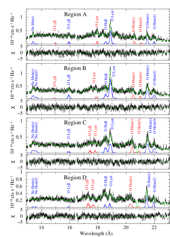
Figure 3: XMM-Newton spectra of the four regions in Figure 1. The RGS1 and RGS2 cover 15.5–24 Å ($\sim$0.8–0.51 keV) and 13–19.1 Å ($\sim$1–0.65 keV), respectively. The two (RGS1 and RGS2) data sets are simultaneously fitted with a combination model of vpshock (for diffuse background emission) + nine Gaussians (for the ejecta knot) + six Gaussians (for the ejecta filament). The total best-fit model is shown in green, while individual components are in blue and red for the ejecta knot and the ejecta filament, respectively. Lower panels show the residuals.

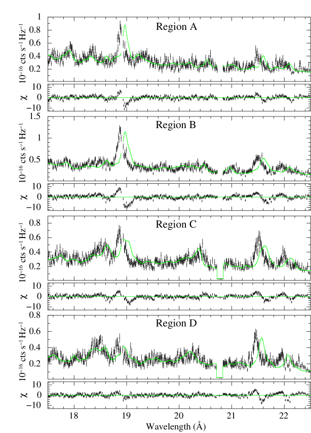
Figure 4: Close-up RGS spectra for O K-shell lines. To clarify the Doppler shifts of the two ejecta features, we here show the best-fit models shifted at rest-frame positions, i.e., redshift = 0. The lower panels show residuals. Blueshifts for O Ly$\alpha$ and O He$\alpha$ for the ejecta knot component are clearly seen.

Figures 3 and 4 shows BG-subtracted RGS1 and RGS2 spectra for the four regions. While most of the emission is due to overall diffuse emission which acts as effective BG emission in our analysis, several peaks can be identified as line emission from our interesting two ejecta features. Some of them are indicated in the plot as blue and red labels for the ejecta knot and the ejecta filament, respectively. Note that there is large wavelength shifts in line centroids between the knot (blue) and the filament (red) by about 1Å. This is mainly due to the off-axis position (about 8^′) of the filament; an offset of 1^′ causes a wavelength shift of 0.138 Å. We use data in the energy range of 0.5–1 keV (24–13 Å) where line emission from the ejecta features are clearly detected. Dividing the energy band into four sections, 0.5–0.6 keV, 0.6–0.7 keV, 0.7–0.85 keV, and 0.85–0.97 keV, we generate RGS responses using the same energy-band images. We note that the available energy ranges for the RGS1 and the RGS2 are limited to 0.5–0.8 (24–15.5 Å) and 0.65–1 keV (19–13 Å), respectively, since chip #7 in the RGS1 and chip #4 in the RGS2 are no longer operating.

The RGS spectra consist of diffuse emission and emission from the ejecta knot and ejecta filament. We model the diffuse emission and the ejecta in terms of a nonequilibrium ionization shock model (the vpshock model: Borkowski et al., 2001) and individual Gaussian components, respectively. We use nine gaussian components for the ejecta knot and six for the ejecta filament. We impose the Gaussians in the knot component to be O VII He$\alpha$ forbidden at @0.561 keV (22.1 Å), O VII He$\alpha$ intercombination at @0.568 keV (21.8 Å), O VII He$\alpha$ resonance at @0.574 keV (21.6 Å), O VIII Ly$\alpha$ @0.654 keV (19.0 Å), O VII He$\beta$ @0.666 keV (18.6 Å), O VIII Ly$\beta$ @0.775 keV (16.0 Å), Ne IX He$\alpha$ forbidden @0.905 keV (13.7 Å), Ne IX He$\alpha$ intercombination @0.915 keV (13.6 Å), and Ne IX He$\alpha$ resonance @0.922 keV (13.5 Å). The six Gaussians for the filament component are the same O K-shell lines listed above. For the diffuse component, the degradation of RGS spectra is sever owing to the large spatial extent; the effective spectral resolution is much worse than the nondispersive CCDs. Therefor, it is difficult to constrain numerous parameters, hence in our fitting procedure, we only allow the electron temperature, $kT_{\rm e}$, and normalizations to vary freely, fixing the intervening hydrogen column density, $N_{\mathrm{H}}$, to be 3$\times$10²¹ cm^-2 and the range of the ionization timescale, $n_{\rm e}t$, from zero up to 3$\times$10¹¹ cm^-3 s, based on recent X-ray measurements (Hwang et al., 2005, 2008; Katsuda et al., 2010). For the Gaussian components, we allow all normalizations to vary freely. Line centroids are fixed to theoretically expected values (Smith et al., 2001), but we allow a redshift parameter to vary freely, keeping the same value for all Gaussians in either the knot or the filament component. Line broadening of the knot component is a free parameter taken to be proportional to line center energies as is expected for a collisionless shock heating. That of the filament component is set to zero, since line emission from the filament is not very clear in the RGS spectrum. For the knot component in regions A, B, and C, we measure redshift and line broadening separately for the RGS1 and the RGS2, so that we can evaluate systematic uncertainties in our measurements and also see if energy dependence is present; the RGS1 covers 0.5–0.8 keV including O K-shell lines while the RGS2 covers 0.65–1 keV including O and Ne K-shell lines, respectively. Before BG subtraction, each spectrum is grouped into bins with at least $\sim$25 counts, which allows us to perform a $\chi^{2}$ test.

With this fitting strategy, we obtain fairly good fits for all the spectra as shown in Figure 3, where individual knot and filament components are shown in blue and red, respectively, as well as the total model in green. The fit results are summarized in Table 1. Overall, the redshifts and line broadening derived from the RGS1 and the RGS2 are consistent with each other, suggesting no significant energy dependence for these parameters. We also fitted the RGS2 spectra, by using a specific energy band for Ne IX He$\alpha$ lines, finding consistent results as in Table 1. Figure 4 shows close-up RGS spectra for O K-shell lines. In this plot, we show the best-fit models shifted at rest-frame positions (i.e., redshift = 0) in green. The Doppler shifts of the ejecta knot are clearly seen.

The blueshift measured at the southernmost region (region D), 1560$\pm$60$\>\rm{\,km\,s}^{-1}$, is consistent with our previous X-ray measurements (Katsuda et al., 2008), significantly reducing the uncertainty. It also matches with the previous optical measurements for the $\Omega$ filament: 1520$\pm$40 $\>\rm{\,km\,s}^{-1}$ or 1570$\pm$20 $\>\rm{\,km\,s}^{-1}$ from the SIT or CCD spectrum, respectively (Winkler & Kirshner, 1985). While the blueshifts in the four regions are all close with each other, that in the northernmost region is slightly slower than the other regions. This conflicts with our previous measurements that suggested a faster velocity in the north of the knot than that in the south. Given much improved spectral resolution in the current data, we believe that the result presented here is more reliable than the previous one. As for the slightly slower velocity, it may indicate that the northern part is responsible for a tail structure delayed from the main body of the ejecta knot. We find, for the first time, that line emission from ejecta filament is redshifted by $\sim$650$\>\rm{\,km\,s}^{-1}$.

Line broadening in the ejecta knot is found to be fairly narrow. It ranges from 0 to 0.9 eV at 0.654 keV in the four regions, which we take as our measurement uncertainty. Based on the relation between temperatures and line broadening, $\sigma=E_{0}\sqrt{kT/mc^{2}}$ (Rybicki & Lightman, 1979), we obtain an upper limit of an oxygen temperature to be 30 keV.

Line intensity ratios measured are consistent with those expected by a non-equilibrium ionization plasma model. We have indeed confirmed that the vnei model (Borkowski et al., 2001) can also well reproduce the RGS spectra (values of $\chi^{2}$/d.o.f. range from 1.4 to 1.6) with plausible electron temperatures, $\sim$0.4–1 keV, an ionization timescale of 2$\times$10¹⁰$\rm{\,cm}^{-3}\,$s, and both Doppler shifts and line broadening consistent with those in Table 1.

4 MOS Spectra

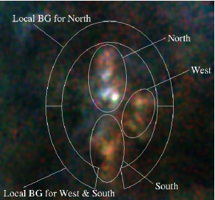
Figure 5: Spectral extraction regions for the MOS data overlaid on a close-up Chandra image shown in Figure 1 right. The local BG regions are also shown.

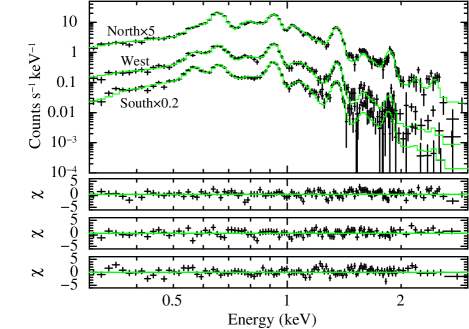
Figure 6: The MOS spectra extracted from the regions shown in Figure 5. The best-fit vnei models are shown together in green. For clarity, the spectra from the north and the south are multiplied by 5 and 0.2 times, respectively. The lower panels are the residuals for north, west, and south from top to bottom, respectively.

Since the RGS spectra are heavily contaminated by the surrounding diffuse emission in our case, electron temperatures and ionization timescales for our interesting features are better constrained by the MOS rather than the RGS. We thus analyze the MOS spectra for the ejecta knot. As shown in a close-up Chandra image in Figure 5, the knot appears to consist of three parts: north, west, and south. We extract spectra from these features. Local BGs are taken from the adjacent regions. We sum up data taken by the MOS1 and the MOS2 to improve photon statistics. The local-BG subtracted MOS1+2 spectra together with the best-fit vnei model (the augmented version 2.0: Borkowski et al., 2001), are presented in Figure 6.

It is difficult to measure absolute (relative to hydrogen) metal abundances for metal-rich plasmas, because continuum emission comes from the metals themselves and no longer reflects the amount of hydrogen, and also because in our case the continuum emission from the ejecta knot is difficult to estimate adequately, given that a considerable fraction of the X-ray emission is due to local BG that cannot be subtracted perfectly. Therefore, in our spectral modeling, we examine two abundance patterns: In case A, we assume the Fe/H abundance to be the solar value (Anders & Grevesse, 1989) as line emission from Fe is not evident in our X-ray spectra, while in case B, we assume the O/H abundance to be 2000 times the solar value which is derived from optical spectroscopy of the $\Omega$ filament (Winkler & Kirshner, 1985). We find that the vnei model represents the data fairly well for both of the two cases. The best-fit models presented in Figure 6 are those for case A which gives slightly better fits than case B. Table 2 summarizes the results and notes details of our fitting.

The blueshifts from the MOS spectra are in reasonable agreements with the RGS measurements, considering the relatively large calibration uncertainty ($\pm$5 eV) on the energy scale of the MOS. We also confirm the elevated abundances of O, Ne, and Mg compared with Fe. On the other hand, the electron temperatures and ionization timescales are outside statistical uncertainties of our previous measurements (Katsuda et al., 2008). The discrepancy would be partly due to the different data quality; the data were taken at the edge (previous) or center (this time) of the FOV, and partly due to the different fitting strategy; we here use (1) the most recent version of the vnei code, (2) different spectral extraction regions, and (3) different energy band, and also we fix $N_{\mathrm{H}}$ to be 3$\times$10²¹ cm^-2 (Katsuda et al., 2010), but allow abundances of C and N to vary freely. Not only these analysis improvements but also the fact that blueshifts derived here are closer to the RGS measurements assure reliability of the current results rather than the previous ones.

Assuming the plasma depths to be 1^′ (or $\sim$0.6 pc at a distance of 2.2 kpc: Reynoso et al., 2003), which is roughly the size of the knot, we calculate densities and masses in each region. Although it is often assumed that a density ratio between electrons and protons to be unity or so, this assumption is incorrect for super-metal rich plasmas like the ejecta knot in Puppis A. Therefore, we here calculate the ratio, taking account of abundances as well as ion fractions based on the SPEX code (Kaastra, et al., 1996). Then, the emission measures and abundances give densities and masses for each species as summarized in Table 3. The total mass in each region, $\sim$0.01 M_⊙, is consistent with our previous estimates (Katsuda et al., 2008), and is comparable with typical OFMKs in the remnant (Winkler et al., 1988).

5 Discussion

The XMM-Newton RGS allowed successful measurements of accurate Doppler velocities of two X-ray–emitting ejecta features (i.e., the ejecta knot and the ejecta filament) in the NE quadrant of Puppis A. In our spectral analysis, we divided each feature into four cross-dispersion regions. The error-weighted mean Doppler velocities for the four regions are obtained to be 1480$\pm$140$\pm$60$\>\rm{\,km\,s}^{-1}$ blueward for the ejecta knot and 650$\pm$70$\pm$60$\>\rm{\,km\,s}^{-1}$ redward for the ejecta filament, where the first and second term errors, respectively, represent the standard deviation for the four regions and a wavelengths accuracy of the RGS. The Doppler velocity of the ejecta knot is fully consistent with previous optical measurements for the $\Omega$ filament (Winkler & Kirshner, 1985), ensuring robustness of our measurements.

The RGS spectra also enabled, for the first time, to measure broadening of O (and Ne) K-shell lines of the ejecta knot. The broadening is found to be modest, $\sigma\lesssim 0.9$ eV at O VIII Ly$\alpha$, indicating an upper limit of an oxygen temperature of 30 keV. As far as we know, this is the second result that we were able to measure an oxygen temperature of fast-moving ejecta knots in X-rays. Comparing our results with the first successful object, a comparably fast-moving ejecta knot in the northwestern rim of SN 1006, we notice that the oxygen temperature in Puppis A’s knot is at least an order-of-magnitude lower than that in SN 1006’s knot ($kT_{\rm O}\sim$300 keV: Vink et al., 2003; Broersen et al., 2013).

The post-shock temperature, $T_{i}$, for species $i$ with mass $m_{i}$ right behind a collisionless shock in the absence of the magnetic pressure is given as (e.g., Spitzer, 1965):

$$kT_{i}=\frac{3}{16}m_{i}v_{\rm sh}^{2}$$ (1)

for shock velocity, $v_{\rm sh}$. Thus, the particles will have mass-proportional temperatures in the limit of collisionless plasma. In fact, the high oxygen temperature together with a relatively low electron temperature of $\sim$1.5 keV in SN 1006 has been reasonably interpreted as evidence for temperature nonequilibration between ions and electrons after collisionless shock heating. As for Puppis A’s knot, the oxygen temperature is expected to be $\sim$130 keV, if we assume that the shock velocity is similar to the gas velocity: $\sim 2000$$\>\rm{\,km\,s}^{-1}$derived by the Doppler velocity of $\sim 1500$$\>\rm{\,km\,s}^{-1}$and the optical proper motion of $\sim$1250$\>\rm{\,km\,s}^{-1}$ at a distance of 2.2 kpc (Winkler et al., 1988; Garber et al., 2010; Reynoso et al., 2003). This prediction conflicts with our measurement, $kT_{\rm O}\lesssim$30 keV.

To understand the apparent temperature inconsistency between the measurement and the simple prediction above, we are required to inspect heating processes at the collisionless shocks. In fact, it is well known that temperatures measured in the immediate post-shock regions do not often obey Equation 1 (Ghavamian et al., 2007; Vink, 2012, for a recent review). The deviation may be due to plasma processes that raise an electron temperature at (in front of) the shock (Ohira et al., 2008; Rakowski et al., 2008) and/or significant energy leakage into cosmic rays that lowers post-shock temperatures of all particle species (Hughes et al., 2000; Helder et al., 2009). In any case, oxygen can have a lower temperature than that predicted by Equation 1.

In this context, it is important to clarify whether the $T_{\mathrm{O}}$/$T_{\mathrm{e}}$ ratio observed in Puppis A’s knot can be explained by temperature equilibration due to Coulomb interactions behind a collisionless shock or requires other scenarios. To this end, assuming pure collisionless shock heating, i.e., initial temperatures are given by Equation 1, we solve the following temperature equilibration due to Coulomb interactions (e.g., Spitzer, 1965):

$$\frac{dT_{i}}{dt}=\frac{T_{j}-T_{i}}{t_{\rm{eq}(i,j)}},~{}~{}t_{\rm{eq}(i,j)}=5.87\frac{A_{i}A_{j}}{n_{j}Z_{i}^{2}Z_{j}^{2}\rm{ln(\Lambda)}}\left(\frac{T_{i}}{A_{i}}+\frac{T_{j}}{A_{j}}\right)^{\frac{3}{2}}$$ (2)

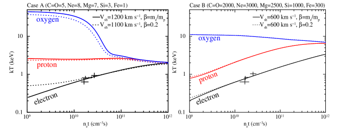
Figure 7: Temperature histories for electrons (black), protons (red), and oxygen (blue) as a function of $n_{\rm e}t$. The models are calculated for two initial electron-to-proton temperature ratios, $\beta$, of the mass ratio (solid curve) and 0.2 (dotted curve). The crosses are electron temperatures and ionization timescales measured for the three regions in the ejecta knot (see, Table 2). Left and right panels are calculated for case A (several-solar abundances as indicated on top of the plot) and case B (super-solar abundances), respectively.

for species $i$ and $j$ with atomic numbers $A_{i}$ and $A_{j}$, charges $Z_{i}$ and $Z_{j}$, number density $n_{j}$, and the Coulomb logarithm ln($\Lambda$) $\sim$ 40. We coupled the differential equations for electrons, protons, He, C, O, Ne, Mg, Si, and Fe, using the abundances for either case A (He/H=1, C/H=O/H=5, Ne/H=8, Mg/H=7, Si/H=3, and Fe/H=1 times the solar values, see Table 2) or case B (He/H=1, C/H=O/H=2000, Ne/H=3000, Mg/H=2500, Si/H=1000, and Fe/H=300 times the solar values). After examining several shock velocities, we find that the electron temperatures and ionization timescales in the ejecta knot can be best explained at $v_{\rm sh}\sim 1200$$\>\rm{\,km\,s}^{-1}$ or $v_{\rm sh}\sim 600$$\>\rm{\,km\,s}^{-1}$ for case A or case B, respectively. The temperature histories for electrons, protons, and oxygen as a function of $n_{\rm e}t$ are shown in Figure 7. From the plot, we also find that the oxygen temperature measured, $T_{\rm O}\lesssim 30$ keV, is consistent with the expectation in both cases. Therefore, we do not need to invoke some exotic scenarios to explain the low $T_{\rm O}/T_{\rm e}$ ratio.

Still, the temperatures measured may be also reproduced for the case that initial post-shock temperatures are not proportional to particle masses, as is often observed. If it is the case, the shock velocities would be different, causing uncertainties on the shock velocity. Recent observational studies agree in that the initial electron-to-proton temperature ratio, $T_{\rm e}/T_{\rm p}=\beta$, is close to unity (full equilibration) for slow shocks ($v_{\rm sh}\lesssim$400$\>\rm{\,km\,s}^{-1}$), but gradually goes down for faster shocks (Ghavamian et al., 2007; Heng, 2010, and references therein). We take the value of $\beta$ to be 0.2 which is typical around $v_{\rm sh}=1000$$\>\rm{\,km\,s}^{-1}$ (van Adelsberg et al., 2008). We find that temperature histories expected at $v_{\rm sh}\sim 1000$$\>\rm{\,km\,s}^{-1}$ (case A) or $v_{\rm sh}\sim 600$$\>\rm{\,km\,s}^{-1}$ (case B), indicated as dotted lines in Figure 7, best match our measurements. In this context, we argue that the shock velocity does not depend on the degree of initial temperature equilibration compared with the ambiguity of abundances.

It is interesting to note that the inferred shock velocity, 600–1200$\>\rm{\,km\,s}^{-1}$, is less than the shocked-gas velocity, $\sim 2000$$\>\rm{\,km\,s}^{-1}$. This suggests that the ejecta knot was heated by a reverse shock rather than a forward shock, since the forward shock velocity should be $\sim$2500$\>\rm{\,km\,s}^{-1}$according to the Rankine-Hugoniot relation:

$$v_{\rm fs}=\frac{\gamma+1}{2}v_{\rm sg},$$ (3)

where $v_{\rm fs}$ and $v_{\rm sg}$ are velocities of the forward shock and the shocked gas, respectively, and $\gamma$ is the specific heat ratio taken to be 5/3 for a non-relativistic ideal gas. The Rankine-Hugoniot relation over the reverse shock can be written down as:

$$v_{\rm free}-v_{\rm rs}=\frac{\gamma+1}{\gamma-1}\left(v_{\rm sg}-v_{\rm rs}\right),$$ (4)

where $v_{\rm free}$ and $v_{\rm rs}$ are velocities of the freely-expanding ejecta and the reverse shock in the observer’s frame. Substituting $v_{\rm free}-v_{\rm rs}$ (=$v_{\rm sh}$) = 600–1200$\>\rm{\,km\,s}^{-1}$, $v_{\rm sg}=$ 2000$\>\rm{\,km\,s}^{-1}$, and $\gamma=5/3$, we compute the value of $v_{\rm free}$ to be 2900–2450$\>\rm{\,km\,s}^{-1}$, depending on the shock velocity of 600–1200$\>\rm{\,km\,s}^{-1}$. This velocity agrees with a typical ejecta velocity in O-rich layer for Type IIb SN (Houck & Fransson, 1996; Iwamoto et al., 1997) which is likely the origin of Puppis A (Chevalier, 2005). Also, the distance, 0.3–0.6 pc, that the shock of this velocity travels for $\sim$500 years (which is a product of the ionization timescale, 3$\times 10^{10}$$\rm{\,cm}^{-3}\,$s, divided by the electron density, 2 cm^-3, as in Tables 2 and 3) is comparable with the size of the knot ($\sim$0.6 pc), showing self-consistency of our interpretation.

We comment on the remarkable difference in $T_{\rm O}/T_{\rm e}$ between Puppis A’s knot and SN 1006’s knot. The proper motion of SN 1006’s knot is measured from recent X-ray observations to be $\sim$3000$\>\rm{\,km\,s}^{-1}$ (Katsuda et al., 2013). Provided that it is shocked by a forward shock, then the shock velocity would be the proper motion itself. On the other hand, if it is shocked by a reverse shock, the proper motion should be the velocity of the shocked gas. Also, freely-expanding ejecta velocities is likely $\sim$10000$\>\rm{\,km\,s}^{-1}$ (Iwamoto et al., 1999), since there is a general consensus that SN 1006 is a Type Ia SNR. This is indeed comparable to a freely-expanding Si-rich ejecta velocity of $\sim$7000$\>\rm{\,km\,s}^{-1}$ measured by the UV absorption edge (Hamilton et al., 2007) as well as a simple estimate from the radius at the knot ($\sim$9 pc) and the SNR age ($\sim$1000 yr). Then, Equation 4 gives the reverse shock velocity in the ejecta-rest frame to be $\sim$9300$\>\rm{\,km\,s}^{-1}$(or $\sim$5300$\>\rm{\,km\,s}^{-1}$, if we take $v_{\rm free}$ to be 7000$\>\rm{\,km\,s}^{-1}$). Therefore, the shock velocities estimated for SN 1006’s knot are at least a few times faster than that for Puppis A’ knot. In addition, the ionization timescale is an order-of-magnitude lower in SN 1006’s knot than in Puppis A’ knot. These differences can qualitatively explain the different oxygen temperatures.

Future high-resolution X-ray spectroscopy with the nondispersive soft X-ray spectrometer onboard Astro-H (FWHM$\sim$5 eV: Takahashi et al., 2010; Mitsuda et al., 2010) will reveal ion and electron temperatures for many SNRs. Hopefully, we will be able to measure ion temperatures in different ionization states for every species. Such information will significantly improve our understanding on temperature equilibration for fast collisionless shocks. One particularly interesting target in Puppis A would be the Si-rich clump in the NE remnant (Hwang et al., 2008), for which the RGS cannot produce high-resolution spectra due to its large angular size (3${}^{\prime}\times 5^{\prime}$). Fortunately, this target is scheduled to be observed in 2013 January with a soft X-ray spectrometer onboard the Micro-X sounding rocket experiment (FWHM$\sim$2 eV: Figueroa-Feliciano et al., 2012). This experiment will provide exciting results shortly.

6 Summary

We have presented results from our new XMM-Newton RGS and MOS observations of two ejecta features in the Galactic SNR Puppis A: one is an ejecta knot positionally coincident with the optical $\Omega$ filament (Winkler & Kirshner, 1985), and the other is an ejecta filament located near the NE edge of the remnant. The results obtained are summarized below:

• The Doppler velocity of the ejecta knot is measured to be 1480$\pm$140$\pm$60$\>\rm{\,km\,s}^{-1}$ blueward, which is fully consistent with previous optical measurements for the $\Omega$ filament (Winkler & Kirshner, 1985). We find that the Doppler velocities are constant within the knot, except for a northernmost piece where a slightly slower velocity is indicated.

• An upper limit of line broadening for O K-shell lines in the ejecta knot is obtained to be $\sim$0.9 eV, leading to an oxygen temperature of $\lesssim 30$ keV. This upper limit, combined with the electron temperature and the ionization timescale derived from the MOS spectra, suggests that the ejecta knot was heated by a reverse shock whose velocity is $\sim$600–1200$\>\rm{\,km\,s}^{-1}$, without requiring rapid temperature equilibration due to plasma instabilities nor temperature dropping due to energy leakage into cosmic rays.

• The oxygen temperature of the ejecta knot is an order-of-magnitude lower than that obtained in a comparably fast-moving ejecta knot in SN 1006 (Vink et al., 2003; Broersen et al., 2013). We argue that the difference would be due to both different shock velocities and the ionization timescale.

• The Doppler velocity for the ejecta filament is also measured, for the first time, to be 650$\pm$70$\pm$60$\>\rm{\,km\,s}^{-1}$ redward.

Table 1: Spectral-fit paramters derived from the RGS

Component	Parameter	Regions
		A	B	C	D
Knot	Redshift (10-3)	-4.5${}^{+0.3}_{-0.1}$, -4.1${}^{+0.1}_{-0.5}$	-5.0$\pm$0.2, -4.6$\pm$0.2	-5.3${}^{+0.3}_{-0.1}$, -5.3${}^{+0.3}_{-0.1}$	-5.2$\pm$0.2
	Line broadening ($\sigma$ in eV @0.654 keV)	0.0 ($<0.4$), 0.0 ($<0.7$)	0.3${}^{+0.4}_{-0.2}$, 0.9$\pm$0.3	0.0 ($<0.4$), 0.0 ($<0.4$)	0.8$\pm$0.3
	Intensities:  O He$\alpha$ (f)	411$\pm$101	812$\pm$123	882$\pm$126	657$\pm$104
	O He$\alpha$ (i)	6 ($<87$)	0 ($<49$)	113$\pm$104	0 ($<74$)
	O He$\alpha$ (r)	702$\pm$103	1623$\pm$133	1519$\pm$127	1085$\pm$116
	O He$\beta$	157$\pm$30	342$\pm$38	428$\pm$40	134$\pm$33
	O Ly$\alpha$	956$\pm$54	1898$\pm$64	863$\pm$52	220$\pm$37
	O Ly$\beta$	123$\pm$20	247$\pm$24	107$\pm$21	40$\pm$16
	Ne He$\alpha$ (f)	26$\pm$25	115$\pm$29	139$\pm$28	48$\pm$22
	Ne He$\alpha$ (i)	0 ($<6$)	25 ($<54$)	42$\pm$28	9 ($<30$)
	Ne He$\alpha$ (r)	149$\pm$25	216$\pm$29	191$\pm$28	47$\pm$22
Filament	Redshift (10-3)	2.3${}^{+0.2}_{-0.5}$	1.9${}^{+0.4}_{-0.1}$	2.2${}^{+0.1}_{-0.3}$	2.4${}^{+0.4}_{-0.2}$
	Intensities:  O He$\alpha$ (f)	285$\pm$112	489$\pm$118	374$\pm$123	207$\pm$179
	O He$\alpha$ (i)	0 ($<48$)	77 ($<185$)	70 ($<167$)	129$\pm$104
	O He$\alpha$ (r)	459$\pm$101	612$\pm$109	1069$\pm$119	619$\pm$117
	O He$\beta$	26 ($<63$)	28 ($<69$)	213$\pm$38	366$\pm$43
	O Ly$\alpha$	237$\pm$41	167$\pm$40	210$\pm$38	223$\pm$40
	O Ly$\beta$	113$\pm$35	56$\pm$34	0 ($<34$)	0 ($<7$)
Diffuse	$kT_{\mathrm{e}}$ (keV)	0.46$\pm$0.01	0.47$\pm$0.01	0.44$\pm$0.01	0.45$\pm$0.01
$\chi^{2}$/d.o.f.		1937.8 / 1260	2073.0 / 1280	1841.6 / 1260	1875.9 / 1257

Note. — $N_{\mathrm{H}}$ values are fixed to 3$\times 10^{21}$ cm^-2. Line intensities are in units of 10^-5 photons cm^-2 s^-1, respectively. Two values of the redshifts and line broadening in Regions A, B, and C are derived by the RGS1 (left) and the RGS2 (right). The errors represent 90% confidence levels on an interesting single parameter.

Table 2: Spectral-fit parameters derived from the MOS

Parameter	North		West		South
	Case A	Case B	Case A	Case B	Case A	Case B
$kT_{\mathrm{e}}$ (keV)	0.93${}^{+0.15}_{-0.12}$	1.03$\pm$0.12	0.80${}^{+0.09}_{-0.05}$	0.83${}^{+0.06}_{-0.12}$	0.63${}^{+0.13}_{-0.08}$	0.63${}^{+0.16}_{-0.08}$
log($n_{\mathrm{e}}t$/cm${}^{-3}\,$s)	10.43${}^{+0.09}_{-0.06}$	10.40${}^{+0.07}_{-0.06}$	10.24${}^{+0.13}_{-0.07}$	10.23${}^{+0.07}_{-0.02}$	10.21${}^{+0.09}_{-0.06}$	10.22${}^{+0.09}_{-0.11}$
(C/H)/(C/H)⊙	11.9${}^{+8.0}_{-7.0}$	6000${}^{+2400}_{-3800}$	5.6${}^{+6.2}_{-5.6}$	1800$\pm$1800	3.1${}^{+3.6}_{-2.9}$	1500$\pm$1300
(N/H)/(N/H)⊙	0.0 ($<1.2$)	0 ($<300$)	1.8 ($<3.8$)	500 ($<1100$)	1.5${}^{+1.4}_{-1.1}$	700$\pm$500
(O/H)/(O/H)⊙	5.2${}^{+1.1}_{-0.8}$	2000a	6.9${}^{+1.1}_{-0.8}$	2000a	4.5${}^{+1.1}_{-0.8}$	2000a
(Ne/H)/(Ne/H)⊙	6.5${}^{+1.4}_{-1.1}$	2400${}^{+100}_{-200}$	10.3${}^{+2.4}_{-2}$	3000$\pm$200	7.5${}^{+2.2}_{-1.7}$	3400$\pm$300
(Mg/H)/(Mg/H)⊙	5.6${}^{+1}_{-0.9}$	2100$\pm$200	7.9${}^{+0.7}_{-1.2}$	2300$\pm$200	7.2${}^{+1.9}_{-1.5}$	3200$\pm$500
(Si/H)/(Si/H)⊙	3.2$\pm$0.7	1200${}^{+200}_{-100}$	2.8${}^{+1.1}_{-1.2}$	900$\pm$300	4.0${}^{+1.9}_{-1.4}$	1900${}^{+600}_{-500}$
(Fe/H)/(Fe/H)⊙	1a	380${}^{+70}_{-60}$	1a	270${}^{+90}_{-110}$	1a	390${}^{+130}_{-110}$
Redshift ($10^{-3}$)	-6.5${}^{+0.6}_{-0.3}$	-6.6${}^{+1.0}_{-0.1}$	-6.1${}^{+0.3}_{-1.0}$	-6.1${}^{+0.3}_{-1.1}$	-5.4${}^{+1.6}_{-0.2}$	-5.4${}^{+1.0}_{-0.1}$
$n_{\mathrm{e}}n_{\mathrm{H}}V/4\pi d^{2}$ (107cm-5)	740${}^{+130}_{-140}$	1.84${}^{+0.17}_{-0.19}$	240${}^{+60}_{-10}$	0.80${}^{+0.07}_{-0.04}$	460${}^{+170}_{-160}$	1.04${}^{+0.15}_{-0.18}$
$\chi^{2}$/d.o.f.	187.7 / 126	200.6 / 126	141.0 / 103	148.3 / 103	180.8 / 108	192.1 / 108

Note. — ^a(Fe/H)/(Fe/H)_⊙ and (O/H)/(O/H)_⊙ are fixed to 1 (Case A) and 2000 (Case B), respectively. $N_{\mathrm{H}}$ values are fixed to 3$\times 10^{21}$ cm^-2. The errors represent 90% confidence levels.

Table 3: Densities (10^-4 cm^-3) and Masses (10^-4 M_⊙) in the ejecta knot

Parameter	North		West		South
	Case A	Case B	Case A	Case B	Case A	Case B
$n_{\rm e}$	44000	11000	33000	7800	37000	7200
$n_{\rm H}$	35000	360	26000	370	29000	340
$n_{\rm C}$	150	770	53	240	33	190
$n_{\rm O}$	150	610	150	620	110	570
$n_{\rm Ne}$	28	110	33	130	27	140
$n_{\rm Mg}$	7.5	28	7.7	31	8.1	41
$n_{\rm Si}$	4.0	15	2.6	11	4.2	23
$n_{\rm Fe}$	1.6	6.3	1.2	4.7	1.4	6.2
$M_{\rm H}$	82	0.8	36	0.5	62	0.7
$M_{\rm C}$	4.3	22	14	4.0	0.8	4.7
$M_{\rm O}$	5.8	23	3.3	14	3.8	19
$M_{\rm Ne}$	1.3	5.0	0.9	3.7	1.1	5.9
$M_{\rm Mg}$	0.4	1.6	0.3	1.0	0.4	2.1
$M_{\rm Si}$	0.3	1.0	0.1	0.4	0.2	1.3
$M_{\rm Fe}$	0.2	0.8	0.1	0.4	0.2	0.7

Note. — Typical errors which are mainly due to the assumption of the plasma depth are about a factor of 2.

References

- Anders & Grevesse (1989) Anders, E., & Grevesse, N. 1989, Acta, 53, 197
- Arnaud (1996) Arnaud, K.A. 1996, in ASP Conf. Ser. 101, Astronomical Data Analysis Software and Systems V ed. G.H. Jacoby & J. Barnes (San Francisco: ASP), 17
- Becker et al. (2012) Becker, W., Prinz, T., Winkler, P.F., Petre, R. 2012, ApJ, 755, 141
- Blair, et al. (1995) Blair, W. P., Raymond, J. C., Long, K. S., & Kriss, G. A. 1995, ApJ, 454, L35
- Blair et al. (2003) Blair, W.P., Sankrit, R., Ghavamian, P., Raymond, J.C., & Morse, J.A. 2003, BAAS, 35, 1266
- Borkowski et al. (2001) Borkowski, K. J., Lyerly W. J., & Reynolds, S. P. 2001, ApJ, 548, 820
- Broersen et al. (2013) Broersen, S., Vink, J., Miceli, M., Bocchino, F., Maurin, G., Decourchelle, A. 2013, A&A, 552, 9
- Charles et al. (1978) Charles, P.A., Culhane, J.L., & Zarnecki, J.C. 1978, MNRAS, 1978, 185, 15
- Chevalier (2005) Chevalier, R.A. 2005, ApJ, 619, 839
- den Herder et al. (2001) den Herder, J. W., et al. 2001, A&A, 365, L7
- Dewey, et al. (2010) Dewey, D. 2010, Space Science Rev. 157, 229
- van der Heyden et al. (2003) van der Heyden, K. J., Bleeker, J. A. M., Kaastra, J. S., & Vink, J. 2003, A&A, 406, 141
- Dubner & Arnal (1988) Dubner, G. M., & Arnal, E. M. 1988, A&AS, 75, 363
- Figueroa-Feliciano et al. (2012) Figueroa-Feliciano, E., et al. 2012, SPIE, 8443, id.84431B-84431B-17
- Garber et al. (2010) Garber, J., Long, K.S., Waite, C.W., & Winkler, P.F. 2010, BAAS, 41, 469
- Ghavamian et al. (2007) Ghavamian, P., Laming, J.M., Rakowski, C.E. 2007, ApJ, 654, L69
- Hamilton et al. (2007) Hamilton, A.J.S., Fesen, R.A. & Blair, W.P. 2007, MNRAS, 381, 771
- Helder et al. (2009) Helder, E.V., et al. 2009, Science, 325, 719
- Heng (2010) Heng, K. 2010, PASA, 27, 23
- Houck & Fransson (1996) Houck, J.C., & Fransson, C. 1996, ApJ, 456, 811
- Hughes et al. (2000) Hughes, J.P., Rakowski, C.E., & Decourchelle, A. 2000, ApJ, 543, L61
- Hui & Becker (2006) Hui, C.Y., & Becker, W. 2006, 2006, A&A, 457, L33
- Hwang et al. (2005) Hwang, U., Flanagan, K. A., & Petre, R. 2005, ApJ, 635, 355
- Hwang et al. (2008) Hwang, U., Petre, R., & Flanagan, K. A. 2008, ApJ, 676, 378
- Iwamoto et al. (1997) Iwamoto, K., Young, T., Nakasato, N., Shigeyama, T., Nomoto, K., Hachisu, I., & Saio, H. 1997, ApJ, 477, 865
- Iwamoto et al. (1999) Iwamoto, K., Brachwitz, F., Nomoto, K., Kishimoto, N., Umeda, H., Hix, W.R., & Thielemann, F-K. 1999, ApJS, 125, 439
- Kaastra, et al. (1996) Kaastra, J. S., Mewe, R., Liedahl, D. A., Singh, K. P., White, N. E., & Drake, S. A. 1996, A&A, 314, 547
- Katsuda et al. (2008) Katsuda, S., Mori, K., Tsunemi, H., Park, S., Hwang, U., Burrows, D. N., Hughes, J. P., & Slane. P. O. 2008, ApJ, 678, 297
- Katsuda et al. (2010) Katsuda, S., Hwang, U., Petre, R., Park, S., Mori, K., & Tsunemi, H. 2010, ApJ, 714, 1725
- Katsuda et al. (2012) Katsuda, S., et al. 2012, ApJ, 756, 49
- Katsuda et al. (2013) Katsuda, S., Long, K.S., Petre, R., Reynolds, S.P., Williams, B.J., & Winkler, P.F. 2013, ApJ, 763, article id. 85
- Mitsuda et al. (2010) Mitsuda, K., et al. 2010, SPIE, 7732, 773211
- Ohira et al. (2008) Ohira, Y., & Takahara, F. 2008, ApJ, 688, 320
- Petre et al. (1982) Petre, R., Kriss, G., A., Winkler, P. F., & Canizares, C. R. 1982, ApJ, 258, 22
- Petre et al. (1996) Petre, R., Becker, C. M., & Winkler, P. F. 1996, ApJ, 465, L43
- Rakowski et al. (2008) Rakowski, C.E., Laming, J.M., & Ghavamian, P. 2008, ApJ, 684, 348
- Reynoso et al. (2003) Reynoso, E. M., Green, A. J., Jhonston, S., Dubner, G. M., Giacani, E. B., & Goss, W. M. 2003, MNRAS, 345, 671
- Rybicki & Lightman (1979) Rybicki G.B., & Lightman A.P. 1979, Radiative processes in astrophysics. Wiley, New York. U
- Smith et al. (2001) Smith, R. K., Brickhouse, N. S., Liedahl, D. A., & Raymond, J. C. 2001, ApJ, 556, L91
- Spitzer (1965) Spitzer, L. (ed.) 1965, Physics of Fully Ionized Gases (Interscience Tracts on Physics and Astronomy; New York, NY: Interscience)
- Strüder et al. (2001) Strüder, L., et al. 2001, A&A, 365, L18
- Takahashi et al. (2010) Takahashi, T., et al. 2010, SPIE, 7732, 77320Z
- Turner et al. (2001) Turner, M. J. L., et al. 2001, A&A, 365, L27
- van Adelsberg et al. (2008) van Adelsberg, M., Heng, K., McCray, R., & Raymond, J.C. 2008, ApJ, 689, 1089
- Vink et al. (2003) Vink, J., Laming, J. M., Gu, M. F., Rasmussen, A., & Kaastra, J. S. 2003, ApJ, 587, L31
- Vink (2012) Vink, J. 2012, A&AR, 2012, 20, article id. #49
- Winkler & Kirshner (1985) Winkler, P. F. & Kirshner, R. P. 1985, ApJ, 299, 981
- Winkler et al. (1988) Winkler, P. F., Tuttle, J. H., Kirshner, R. P., & Irwin, M., J. 1988, in IAU Colloq. 101: Supernova Remnants and the Interstellar Medium, ed. R. S. Roger & T. L. Landecker, 65
- Winkler & Petre (2007) Winkler, P. F. & Petre, R. 2007, ApJ, 670, 635
- Wongwathanarat et al. (2012) Wongwathanarat, A., Janka, H.-Th., Müller, E. 2012, arXiv1210.8148