Dynamics of strain bifurcations in magnetostrictive ribbon

Abstract

We develop a coupled nonlinear oscillator model involving magnetization and strain to explain several experimentally observed dynamical features exhibited by forced magnetostrictive ribbon. Here we show that the model recovers the observed period doubling route to chaos as function of the dc field for a fixed ac field and quasiperiodic route to chaos as a function of the ac field, keeping the dc field constant. The model also predicts induced and suppressed chaos under the influence of an additional small-amplitude near resonant ac field. Our analysis suggests rich dynamics in coupled order parameter systems like magnetomartensitic and magnetoelectric materials.

I Introduction

The rich chaotic dynamics exhibited by sinusoidally driven nonlinear oscillators is ubiquitous to a large number of systems such as turbulence in fluid systems Gollub75 , chemical oscillators Swinney85 , and cardiac tissues Glass83 . Manipulated properties of chaos, such as control of chaos LR03 realized in driven nonlinear oscillators, are also reported in several disciplines, for instance, control of output of laser system Roy92 , enhanced performance of permanent magnet synchronous motor Liu04 , and control of cardiac arrhythmias Garfinkel92 . Natural to multistate weakly driven oscillators in the presence of ubiquitous noise is the stochastic resonance Benzi81 , another generic noise induced cooperative phenomenon that enhances the signal to noise ratio. This phenomenon is also realized in several disciplines ranging from physics ( e.g., superconducting quantum interference device magnetometers, optical and electronic devises) Gammaitoni98 to biology McDonnell09 . However, it is rare to find such a broad spectrum of dynamical features in a single system. Surprisingly, physical realization of several of these features was reported by Vohra et al. Vohra91a ; Vohra91b ; Vohra94 ; Vohra95 ; Vohra93 . In their study of strain bifurcations in magnetostrictive ribbons subjected to the combined influence of sinusoidal (ac) and dc magnetic fields, the authors reported an extraordinarily large number of dynamical features such as (a) quasiperioidic (QP) route to chaos when the amplitude of the ac magnetic field $h_{ac}$ was increased in the presence of a dc magnetic field $h_{dc}$, (b) period doubling (PD) route to chaos when $h_{dc}$ was increased and the ac field was kept fixed Vohra91a ; Vohra91b , (c) a suppression and shift of period doubling bifurcation point Vohra91b and induced subcritical bifurcation under small-amplitude near-resonant conditions Vohra94 , (d) control of chaos, specifically, suppressed and induced chaos with the application of a near-resonant perturbation to one of the subharmonics Vohra95 , and (e) stochastic resonance Vohra93 . However, modeling such a rich dynamics exhibited by a single system in terms of the relevant strain and magnetic order parameters has remained a challenge.

Vohra et al. emphasize that $\Delta E$ effect Savage86 , i.e., the reversible change in the Young’s modulus with applied magnetic field, is not responsible for the reported dynamics as the samples used are unannealed ribbons where the $\Delta E$ effect is insignificant, unlike the earlier reported PD and QP routes to chaos in the annealed metallic glass samples Ditto89 . Some of these features have been explained using appropriate normal forms Bryant86 by appealing to the universal nature of the bifurcation phenomenon. Our purpose is to develop a model in terms of magnetic and strain order parameters. In this paper we focus on three different experimentally observed dynamical features and show that the model predicts (i) the period doubling and (ii) quasiperiodic routes to chaos and (iii) induced and suppressed chaos in the presence of small-amplitude near-resonant perturbation. The general nature of these equations suggest much richer dynamics in ferromagnetic martensite samples that posses even stronger elastic and magnetic nonlinearities FMM and also in magnetoelectric materials Flebig02 . The model also explains some old results on internal friction studies of martensites Suzuki80 .

II The Model

Experiments were performed using a sinusoidal magnetic field $h_{ac}$ of frequency $\omega$ in the presence of a dc magnetic field $h_{dc}$. Our starting point is to write down the relevant free energies. In general, elastic free energy is a function of all components of the strain tensor. However, considering the fact that the samples are thin long ribbons ($5$cm long) fixed at one end with the displacement or strain being monitored at the other end, it would be adequate to use a single strain order parameter $\epsilon$. Further, we work in one dimension and use dimensionless order parameters. We construct a minimal one-dimensional model with the strain order parameter $\epsilon$ and magnetic order parameter $m$. In our model the weak magnetic nonlinearity is taken to drive the highly nonlinear elastic degrees of freedom Vohra91a . Then the total free energy has three contributions, namely, the strain free energy, magnetic free energy, and magneto-elastic free energy. Thus the total free energy is $F_{T}=F_{\epsilon}+F_{m}+F_{m\epsilon}$.

In one dimension the elastic free energy is given by

$$F_{\epsilon}=\int dy^{\prime}\left(f_{local}(\epsilon(y^{\prime}))+\frac{1}{2}(\frac{\partial\epsilon}{\partial y^{\prime}})^{2}\right),$$ (1)

where the strain variable is $\epsilon=\frac{\partial u(y)}{\partial y}$, $f_{local}$ is the Landau free energy density, and the second term is the gradient free energy. Guided by the normal forms used Vohra91a ; Vohra91b ; Vohra93 ; Vohra94 ; Vohra95 , we use a sixth-order polynomial for the elastic free energy $f_{local}=\frac{\theta}{2}\epsilon^{2}-\frac{\beta}{2}\epsilon^{4}+\frac{\Delta}{6}\epsilon^{6}$. Here $\beta$ is a positive constant, but $\theta$ can take on positive or negative values. To simplify further, we use $\Delta=1$. The minima of the free energy are located at $\epsilon=\pm\epsilon_{s}$ with $\epsilon_{s}=[(\beta+\sqrt{\beta^{2}-\theta})]^{1/2}$. The parameters $\beta$ (of the order of unity) and $\theta$ are sufficient to control the minima. When $\theta\geq 3\beta^{2}/4$, $\epsilon=0$ is the true minima identified with the high-temperature phase. At $\theta=3\beta^{2}/4$, we have a first order transition with the free energy vanishing at $\epsilon^{2}=\pm 3\beta/2$ and $\epsilon=0$. For $\theta$ negative, $\epsilon=0$ state is unstable. This behavior can be parameterized by using $\theta=\frac{T-T_{s}}{T_{f}-T_{s}}=\tau_{\epsilon}$ where $T_{f}$ and $T_{s}$ are the first- and second order transition temperatures, respectively.

The magnetic free energy is given by

$$F_{m}=\int dy^{\prime}\big{[}f_{mag}+\frac{1}{2}(\frac{\partial m}{\partial y^{\prime}})^{2}-m(h_{dc}+h_{ac}\sin\omega t)\big{]},$$

where $f_{mag}=\tau_{c}\frac{m^{2}}{2}+\frac{m^{4}}{4}$ with $\tau_{c}=\frac{T-T_{c}}{T_{c}}$, where $T_{c}$ is the Curie temperature of the sample. The nature of magneto-elastic free energy is not known, particularly since the ribbon is a metallic glass sample with a glassy structure. However, coupling terms either preserve or break the invariance $\epsilon\rightarrow-\epsilon$ and $m\rightarrow-m$ in the elastic and magnetic free energies, respectively. In the absence of any information, we model it as a weighted sum of symmetry-preserving and -breaking terms given by

$$F_{m\epsilon}=-\frac{\xi}{2}\int dy^{\prime}[(1-p)\epsilon(y^{\prime})m(y^{\prime})+p\epsilon^{2}(y^{\prime})m^{2}(y^{\prime})]$$ (2)

where $\xi$ is magnetoelastic coupling coefficient and $0\leq p\leq 1$ is an adjustable weight factor. Other types of gradient coupling between $\epsilon$ and $m$ are ignored to keep the model simple. We use the Rayleigh dissipation function Landau to represent the damping of oscillating ribbon when the applied field is removed. This is given by

$$F_{diss}=\frac{\gamma}{2}\int\!\!\left(\frac{\partial\epsilon}{\partial t}\right)^{2}dy^{\prime}.$$ (3)

The kinetic energy is given by $T=\frac{1}{2}\int\left[\frac{\partial u(y^{\prime})}{\partial t}\right]^{2}dy^{\prime}$, where $u(y,t)$ is the displacement variable. Then, using the Lagrangian $L=T-F_{T}$ and the Lagrange equations of motion $\frac{d}{dt}\left(\frac{\delta L}{\delta\dot{u}(y)}\right)-\frac{\delta L}{\delta{u}(y)}={-\frac{\delta F_{diss}}{\delta\dot{u}(y)}}$, we get

$$\frac{\partial^{2}\epsilon(y)}{\partial t^{2}} = \frac{\partial^{2}}{\partial y^{2}}\Big{[}\tau_{\epsilon}\epsilon(y)-2\beta\epsilon^{3}(y)+\epsilon^{5}(y)-\frac{\partial^{2}}{\partial y^{2}}\epsilon(y)$$ (4)

$$+ \gamma\frac{\partial\epsilon(y)}{\partial t}-\xi\big{(}p\epsilon(y)m^{2}(y)+\frac{(1-p)}{2}m(y)\big{)}\Big{]}.$$

Using the equation of motion for the magnetic order parameter given by $\frac{\partial m}{\partial t}=-\Gamma\frac{\delta F_{T}}{\delta m}$, we get

$$\frac{\partial m(y)}{\partial t} = -\Gamma\Big{[}\tau_{c}m(y)+m^{3}(y)-\frac{\partial^{2}m(y)}{\partial y^{2}}-h_{dc}$$ (5)

$$- h_{ac}\sin\omega t-\xi\Big{(}p\epsilon^{2}(y)m(y)+\frac{(1-p)}{2}\epsilon(y)\Big{)}\Big{]},$$

where $\Gamma$ is a relevant time scale. Note that this is not a pure relaxational dynamics as $m(y)$ is subject to sinusoidal and dc fields. Indeed, $\epsilon(y)$ is being driven through $m(y)$, which is subject to the sinusoidal field. [Note also the mutual coupling between $m(y)$ and $\epsilon(y)$.] For a sample that is clamped at one end, the above equations can be further simplified by noting that the strain at the free end is small even though it is in the anharmonic regime. Thus we assume that only the dominant mode of vibration is supported. We use $\epsilon(y,t)=A(t)\sin ky$ and $m(y,t)=B(t)\sin ky$, where $k=\pi/2L$, with $L$ representing the length of the ribbon. Further, we note that the dc field induces a finite strain value, which can be determined by equating the strain energy with the magnetic energy. The application of the ac magnetic field induces oscillations around this strain value. Thus we use the dominant mode to represent deviation from the equilibrium value of the dc field, i.e., $A=a-a_{dc}$. Here, $a$ is the strain amplitude in the presence of both magnetic fields and $a_{dc}$ is that when only the dc field is imposed. Transforming Eqs.(4,5) into rescaled variables ($\tau=kt,\Omega=\omega/k,\Gamma^{\prime}=\Gamma/k$) and using only the dominant mode, we get

$$\ddot{A}(\tau) = -\Big{[}\tau_{\epsilon}A(\tau)+3\beta A^{3}(\tau)-\frac{5}{8}A^{5}(\tau)+k^{2}A(\tau)$$ (6)

$$+k\gamma\dot{A}(\tau)+\frac{\xi}{2}\Big{(}3pA(\tau)B^{2}(\tau)-(1-p)B\big{)}\Big{]},$$

$$\dot{B}(\tau) = -\Gamma^{\prime}\Big{[}\tau_{c}B(\tau)+\frac{B^{3}(\tau)}{2}+k^{2}B(\tau)-\frac{\xi}{2}\Big{(}(1-p)A$$ (7)

$$+pA^{2}(\tau)B(\tau)\Big{)}-h_{ac}\sin\Omega\tau-h_{dc}\Big{]}.$$

The overdot now refers to the redefined time derivative. Equations (6) and (7) constitute a coupled set of nonlinear nonautonomous ordinary differential equations with several parameters. We shall use $\tau_{\epsilon},\tau_{c},\gamma,\Gamma^{\prime},\Omega$, and $\xi$ as free parameters. In addition, both $h_{ac}$ and $h_{dc}$ are the experimental drive parameters. Apart from this, we have no knowledge of the values of the parameters.

III Results

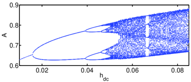
Figure 1: (Color online) Period-doubling bifurcation as a function of $h_{dc}$ for $\tau_{c}=-0.2,\tau_{\epsilon}=-1.0,\Omega=1,\xi=0.6,\gamma=1.592,\Gamma^{\prime}=0.09,h_{ac}=10.5$, and $p=0.32$.

The dynamics of the above system of equations is quite complicated due to the presence of several parameters. Clearly, interesting dynamics can be expected when $\tau_{\epsilon}$ is in the range where three or two minima exist and when $\tau_{c}$ is negative. Thus we first map-out the region of the parameter space where interesting dynamics is seen.

Consider the period-doubling route as a function of $h_{dc}$ for a fixed $h_{ac}$. Here, we keep $\tau_{\epsilon}=-1$ so that $\epsilon=0$ state is unstable, although interesting dynamics is also observed for $\tau_{\epsilon}<3\beta^{2}/4$ as well. Other parameters are fixed at $\tau_{c}=-0.2,\Omega=1,\gamma=1.592,\Gamma^{\prime}=0.09,L=5,\xi=0.6$, and $p=0.32$.

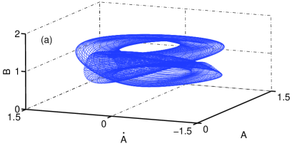
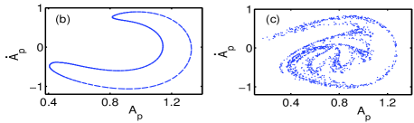
Figure 2: (Color online)(a) Quasiperiodic orbit in the $(\dot{A},A,B)$ space for $h_{ac}=4.8$ keeping $\tau_{c}=-0.2,\tau_{\epsilon}=-1.0,\Omega=0.97,\gamma=0.0421,\xi=3.2,\Gamma^{\prime}=0.09,h_{dc}=0.04$, and $p=0.32$. (b) The corresponding Poincaré map in the $(A_{p},\dot{A}_{p})$ plane. (c) Poincaré map for a chaotic orbit for $h_{ac}=7.4$.

The application of the dc field in the presence of ac field has two effects. First, the vibrations are centered around the strain induced by the dc field. This has already been included in the definition of $A$. Second, the free energy for the magnetic order parameter is tilted to one side. In addition, the shape of the free energy is also affected due to the presence of nonlinear magnetoelastic coupling. In particular, note that apart from the additive $B$ term in Eq. (6), $B^{2}$ appears multiplicatively with $A$ (equivalent to parametric forcing). This affects the shape of the effective elastic free energy. Thus we should expect $\beta$ to be a function of $h_{dc}$. To understand this, we first note that in the absence of $h_{dc}$, increasing the amplitude of the ac field gives period-doubling bifurcation, as expected from studies on Duffing-like oscillators Musielak05 . Increasing $\beta$ also leads to period-doubling sequence keeping $h_{dc}=0$, but keeping $h_{ac}$ at a value where we find period one. In contrast, keeping $h_{ac}$ at a values where chaos is seen (with $\beta=1$) and increasing $h_{dc}$ reverses the period doubling sequence, reflecting the compensating relationship between $\beta$ and $h_{dc}$. This can be made quantitative by keeping $h_{ac}=9.2$ (a value corresponding to a period-four orbit) and increasing both $h_{dc}$ and $\beta$ such that we always see the period-four orbit. This gives a relation $\beta=1+10h_{dc}$. However, while $\beta$ is linear in $h_{dc}$, the prefactor depends on the value of $h_{ac}$ used.

For further calculations, we use this parameterized form of $\beta$ in Eqs.(6,7). Then, increasing $h_{dc}$ and keeping $h_{ac}=10.5$ leads to period-doubling route to chaos. All quantitative measures are obtained after discarding the first $1.5\times 10^{5}$ time steps. A plot of PD sequence is shown in Fig. 1. The PD route is seen for a range of parameter values around those used for Fig. 1.

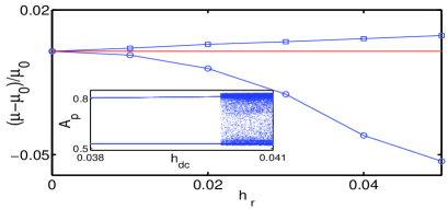
Figure 3: (Color online) Suppressed and induced chaos for $\delta=10^{-6}(\square)$ and $\delta=10^{-2}(\circ)$ respectively as a function of $h_{r}$. The inset shows the bifurcation diagram for $\tau_{c}=-0.2,\tau_{\epsilon}=-1.0,\xi=1.0,\Omega=1,\gamma=1.592,\Gamma^{\prime}=0.09,h_{ac}=10.5$, and $p=0.32$.

Now consider quasiperiodic route to chaos. For this case we choose the driving frequency to be less than that for the period-doubling route ($\Omega=1$). For the results reported here $\Omega=0.97$, but the similar results are obtained for a range of values of $\Omega$ less than unity. We retain most values of the parameters as in the PD sequence, but use higher coupling $\xi=3.2$ and $\gamma=0.0421$. In this case, keeping $h_{dc}=0.04$ fixed, we sweep $h_{ac}$ from $2$ onwards. We find the first few harmonic frequencies (as found in turbulence of rotating fluid; see Ref. Gollub75 ) in the region $h_{ac}=2.5$ to $3.8$, beyond which quasiperiodicty is seen until $5.1$ with the emergence of two incommensurate frequencies. A plot of the torus in the $(A,\dot{A},B)$ space is shown in Fig. 2(a) for $h_{ac}=4.8$. The corresponding Poincaré map in the $(A_{p},\dot{A}_{p})$ plane is shown in Fig. 2(b). (The largest Lyapunov exponent vanishes in the regions of quasiperiodicity.) We find three regions of chaos interrupted by windows of quasiperiodicity in the interval $h_{ac}=2.0$ to $7.5$. The first region of chaos is seen between $h_{ac}=5.45$ to $5.53$ preceded by a phase locked region. This is followed by a transition to quasiperiodic regime ($h_{dc}=5.53-5.64$) followed by an abrupt transition to chaos ($h_{dc}=5.64-5.73$). Another region of chaos is seen for $h_{ac}=7.3-8.0$. The Poincaré map for the chaotic region ($h_{ac}=7.4$ ) is shown in Fig. 2(c). The QP route to chaos is observed for a range of values of parameters around the values used for Fig. 2.

We next examine the possibility of induced and suppressed chaos when the system is subjected to small-amplitude near-resonant perturbation of the form $h(\tau)=h_{r}\sin\Omega_{r}\tau$, with $\Omega_{r}$ close to the first or the second subharmonic. For illustration we use $\Omega_{r}=\Omega/2-\delta$, keeping $\delta$ small. To do this we first locate a direct transition from period-two cycle to chaos as a function of $h_{dc}$, keeping perturbing field $h_{r}=0$. We find that this transition occurs when $h_{dc}=0.04014$ (except for $\xi=1.0$, all other parameters values are the same as for PD route). A bifurcation diagram for the strain amplitude is shown in the inset of Fig. 3. Keeping $h_{dc}=0.04014$, we apply the perturbing signal $h_{r}\sin\Omega_{r}\tau$ with $\delta=10^{-6}$. Even for small $h_{r}$ we find that the onset of chaos is delayed. Further, the magnitude of the shift, though small, increases linearly with $h_{r}$. Identifying $\mu_{0}$ with the onset of chaos ($h_{dc}=0.04014$) when $h_{r}=0$ and $\mu$ with that for finite $h_{r}$, the normalized shift ($\square$) $\frac{\mu-\mu_{0}}{\mu_{0}}$ for the onset of chaos (obtained by computing the Lyapunov exponent) as function of $h_{r}$ is shown in Fig. 3. We have also studied the influence of $\delta$ on the nature of the dynamics. For instance, for $\delta=10^{-2}$, we find induced chaos. The magnitude of the shift in the onset of chaos ($\circ$), which is significantly higher than that for the suppressed chaos, is shown in Fig. 3.

IV Summary and Conclusions

In summary, we have developed a coupled oscillator model where the weak magnetic nonlinearity drives the highly nonlinear strain order parameter. The model explains several experimental results on the dynamics of the magnetostrictive ribbon such as (a) the period-doubling bifurcation as a function of $h_{dc}$ and keeping $h_{ac}$ fixed, (b) the quasiperiodic route to chaos as a function of $h_{ac}$ for a fixed dc field, and (c) induced and suppressed chaos under the influence of the resonant perturbing field $h_{r}$ Vohra91a ; Vohra91b ; Vohra93 ; Vohra94 ; Vohra95 . However, the suppressed chaos seen here is for small $\delta$ while induced chaos is seen for large $\delta$, which is the opposite of what has been reported. This may be attributed to parametric type of forcing in our equations. Note that the method of control of chaos is different from traditional methods LR03 . The model demonstrates induced and suppressed chaos in the presence of near-resonant perturbation. The model exhibits rich dynamics including transient chaos. For instance, for the symmetry restoring crisis LABEL:Ishii86, we find that the mean time $<\tau>$ spent in the precrisis attractor scales as $<\tau>\sim(h_{ac}-h_{ac}^{c})^{-\eta}$, where $h_{ac}^{c}$ is the critical value, with $\eta\sim 1.06$.

The approach is clearly applicable to any coupled order parameter system FMM ; Flebig02 such as magnetomartensites FMM , which exhibits high elastic strain and magnetization, and ferroelectromagnetic materials, which exhibit magnetization and electric polarization Flebig02 . Such systems are also described by polynomial forms of free energy, as used in the model. Our analysis suggests rich dynamics if experiments are performed in a similar geometry on these materials. This should encourage dynamic experiments in these materials where experiments are traditionally carried out in quasistatic conditions.

The model has been adopted to explain some old unexplained results Ritupan11 in the internal friction experiments on samples of nonmagnetic martensite samples of $Cu_{82.9}Al_{14.1}Ni_{3}$ reported Suzuki79 ; Suzuki80 . These experiments have also been carried out in a similar geometry (but transverse drive) near martensite transformation temperature $T_{m}$, where the elastic nonlinearities are significant. Our equations automatically describe the twinned structure in one dimension when the magnetic free-energy contribution is dropped Bales . The model recovers all results Ritupan11 including the period four cycle (which the authors even fail to recognize; see Fig. 2 of Suzuki80 ).

These equations in their present form describe the dynamics of magnetomartensites as well FMM . These alloys undergo a first-order martensitic transformation on cooling below $T=T_{m}$ and are also ferromagnetic below the Curie temperature $T_{c}$. Below $T_{m}$ and $T_{c}$ they have high degree of elastic and magnetic nonlinearities. Indeed, the application of a small amount of magnetic field induces large strains by the rearrangement of martensite variants FMM . Similarly, stress also affects magnetization, thereby suggesting strong magnetoelastic coupling. Thus a rich dynamics is predicted in magnetomartensites if experiments are performed in a similar geometry. It would be interesting to verify this prediction.

Finally, since the application of magnetic field can induce large strains (as high as $\sim 10\%$), magnetomartensites are better suited for actuator applications than even the best magnetostrictive materials (such as Terfenol-D, with a strain of $\sim 0.2\%$ ). Further, these materials should provide more accurate control of the measurement of dynamic strains compared to magnetostrictive materials Vohra94 .

- (1) J. P. Gollub and H. J. Swinney, Phys. Rev. Lett. 35, 927 (1975).
- (2) J. Maselko and H. L. Swinney, Phys. Scr. T9, 35 (1985).
- (3) L. Glass et al., Physica D 7, 89 (1983).
- (4) M. Lakshmanan and S. Rajasekar, Nonlinear Dynamics, Integrability, Chaos and Pattern Formation (Springer-Verlag, Heidelberg, 2003).
- (5) R. Roy, T. W. Murphy, T. D. Maier, Z. Gills, and E. R. Hunt, Phys. Rev. Lett. 68, 1259 (1992).
- (6) D. Liu, H. P. Ren and X.Y. Liu, Proceedings of the 2004 International Symposium on Circuits and Systems, 2004, ISCAS ’04 [IEEE Circuits Syst. 4, 732 (2004)].
- (7) A. Garfinkel et al., Science 257, 1230 (1992).
- (8) R. Benzi, A. Sutera and A. Vulpiani, J. Phys. A 14, L453 (1981).
- (9) L. Gammaitoni et al., Rev. Mod. Phys. 70, 223 (1998).
- (10) M. D. McDonnell and D. Abbott, PLoS Comput. Biol. 5, e1000348 (2009).
- (11) S. T. Vohra et al., J. Appl. Phys. 69, 5736 (1991).
- (12) S. T. Vohra, F. Bucholtz, K. P. Koo, and D. M. Dagenais, Phys. Rev. Lett. 66, 212 (1991).
- (13) S. T. Vohra, L. Fabiny, and K. Wiesenfeld, Phys. Rev. Lett. 72, 1333 (1994).
- (14) S. T. Vohra, L. Fabiny, and F. Bucholtz, Phys. Rev. Lett. 75, 65 (1995).
- (15) S. T. Vohra and F. Bucholtz, Phys. Rev. Lett. 70, 1425 (1993); S. T. Vohra and L. Fabiny, Phys. Rev. E 50, R2391 (1994).
- (16) H. T. Savage and C. Adler, J. Magn. Magn. Mater. 58, 320 (1986).
- (17) W. L. Ditto et al., Phys. Rev. Lett. 63, 923 (1989).
- (18) P. Bryant and K. Wiesenfeld, Phys. Rev. A 33, 2525 (1986).
- (19) See, for example, R. Kainuma et al., Nature 439, 957 (2006), and the references therein.
- (20) M. Fiebig et al., Nature (London) 419, 818 (2002); W. Eerenstein, N. D. Mathur, and J. F. Scott, ibid 442, 759 (2006).
- (21) M. Wuttig and T. Suzuki, Scr. Metall. 14, 229 (1980).
- (22) L. D. Landau and E. M. Lifschitz, Theory of Elasticity, 3rd ed. (Pergamon, Oxford, 1986).
- (23) D. E. Musielak, Z. E. Musielak, and J. W. Benner, Chaos Solitons Fractals 24, 907 (2005).
- (24) H. Ishii, H. Fujisaka and M. Inoue, Phys. Lett., A116, 257 (1986).
- (25) R. Sarmah and G. Ananthakrishna (unpublished).
- (26) M. Wuttig and T. Suzuki, Acta Metall. 27, 755 (1979).
- (27) G. S. Bales and R. J. Gooding, Phys. Rev. Lett. 67, 3412 (1991).