C, N, O, and Na Abundances of Cepheid Variables:
Implications on the Mixing Process in the Envelope

Abstract

With an aim of investigating the nature of evolution-induced mixing in the envelope of evolved intermediate-mass stars, we carried out an extensive spectroscopic study for 12 Cepheid variables of various pulsation periods ($\sim$ 2–16 days) to determine the photospheric abundances of C, N, O, and Na, which are the key elements for investigating how the H-burning products are salvaged from the interior, based on 122 high-dispersion echelle spectra ($\sim 10$ per target) of wide wavelength coverage collected at Bohyunsan Astronomical Observatory. Having established the relevant atmospheric parameters corresponding to each phase spectroscopically from the equivalent widths of Fe i and Fe ii lines, we derived C, N, O, and Na abundances from C i 7111/7113/7115/7116/7119, O i 6155–8, N i 8680/8683/8686, and Na i 6154/6161 lines by using the spectrum-synthesis fitting technique, while taking into account the non-LTE effect. The resulting abundances of these elements for 12 program stars turned out to show remarkably small star-to-star dispersions ($\la$ 0.1–0.2dex) without any significant dependence upon the pulsation period: near-solar Fe ([Fe/H] $\sim 0.0$), moderately underabundant C ([C/H] $\sim-0.3$), appreciably overabundant N ([N/H] $\sim$ +0.4–0.5), and mildly supersolar Na ([Na/H] $\sim+0.2$). We conclude the following implications from these observational facts: (1) These CNO abundance trends can be interpreted mainly as due to the canonical dredge-up of CN-cycled material, while any significant non-canonical deep mixing of ON-cycled gas is ruled out (though only a slight mixing may still be possible). (2) The mild but definite overabundance of Na suggests that the NeNa-cycle product is also dredged up. (3) The extent of mixing-induced peculiarities in the envelope of Cepheid variables is essentially independent on the absolute magnitude; i.e., also on the stellar mass.

1 Introduction

As a star is evolved off the main sequence after exhaustion of hydrogen fuels in the core, it increases its radius while the surface temperature drops down, and the deep convection zone is developed, by which part of the nuclear-processed products in the core may be salvaged and mixed into the outer envelope and abundance peculiarities may be observed for some specific elements. By making use of this fact, we can study the physical process in the invisible interior of stars by comparing spectroscopically determined surface abundances with theoretical expectations from stellar evolution calculations.

While considerable progress has been made so far in this field and important observational characteristics are known to be successfully explained by theoretical calculations, discrepancies between the empirically established surface abundances and the prediction from the standard theory are occasionally seen. One of such problems concerns the oxygen abundances in F–G supergiants, which is namely the disagreement between the theoretical prediction (almost normal O) and an apparent deficit often suggested from observations.

In the envelope of such intermediate-mass supergiants, the H-burning (CNO cycle) products are mixed to alter the surface abundances. According to the canonical stellar evolution calculations (e.g., Lejeune & Schaerer 2001), it is essentially the CN-cycled (C$\rightarrow$N reaction) material that is dredged up, while the product of ON-cycle (O$\rightarrow$N reaction; occurring in deeper region of higher $T$) is unlikely to cause any significant abundance change because mixing is not expected to substantially penetrate into such a deep layer; thus the predicted surface abundances are characterized by a deficit in C as well as an enhancement in N, while O is practically unaffected (if only slightly decreased).

On the observational side, however, Luck & Lambert (1981, 1985) reported based on the CNO abundance results of FGK supergiants (including Cepheid variables) that oxygen is mildly deficient relative to the Sun by $\sim$ 0.2–0.4 dex, while C is underabundant by $\sim$ 0.2–1.0 dex and nitrogen is overabundant by $\sim$ 0.2–0.8 dex (both with a large star-to-star dispersion). In such a deficiency of O is real, a non-canonical deep mixing may exist that dredges the ON-cycle product up into the envelope. Yet, Luck & Lambert (1985) did not stick to this solution and discussed several possibilities (e.g., errors in abundance determinations, peculiarities in solar abundances, etc.). Their tentative conclusion was that their absolute abundance determinations may not necessarily be trustworthy, pointing out that the trends of more reliable C/O ratios (from forbidden lines) as well as C/N ratios (from permitted lines) could be explained by canonical dredge-up of CN-cycled material (though its amount may be more severe than expected). Thus, the problem remained as an open question.

Meanwhile, Takeda and Takada-Hidai published a series of papers in 1990s (Takeda & Takada-Hidai 1994, 1995, 1998, 2000), where the abundance peculiarities of supergiants in terms of Na, N, O, and C were investigated by taking into account the non-LTE effect, though they did not pay much attention to determination of atmospheric parameters (appropriate values corresponding to the spectral type and the luminosity class were simply assumed). One of the important results they first learned was the confirmation of Na enrichment (Takeda & Takada-Hidai 1994), which is regarded as an evidence for the dredge-up of NeNa-cycle product (cf. Sasselov 1986, Lambert 1992). Since such a peculiarity in Na was not expected from canonical stellar evolution calculations, it implied an instructive fact that the standard theory was not necessarily sufficient.

Regarding CNO, Takeda & Takada-Hidai (1998) confirmed the mild underabundance of O by $\sim 0.3$ dex, interestingly just like Luck & Lambert (1985) reported, along with the enrichment of N (Takeda & Takada-Hidai 1995) as well as the deficit of C (Takeda & Takadai-Hidai 2000; though only for late-B through late-A supergiants). But Takeda & Takada-Hidai (1998) did not associate this result of subsolar O with non-canonical mixing of ON-cycled material but attributed it to the general tendency of apparently subsolar CNO observed in young stars such as B-type stars (e.g., Nissen 1993), which was generally accepted (though puzzled) at that time. However, an extensive non-LTE study on the oxygen abundances of B-type stars in comparison with the Sun recently carried out by Takeda et al. (2010) lead to the conclusion that B stars have almost the solar composition in terms of O without any significant difference. If so, these previous studies may point to the conclusion that O is apparently underabundant in supergiants while primordial O must have been almost normal when they were born. Does this imply that oxygen abundance in the envelope of intermediate-mass stars really got decreased during the course of evolution by a non-standard deep mixing of ON-cycled product?

In the meantime, Kovtyukh & Andrievsky (1999) suggested a possible key to the solution of this oxygen problem. According to them, the atmospheric parameters adopted by previous investigations may not have been appropriate, since spectroscopically determined parameters based on Fe i and Fe ii lines tend to suffer to appreciable errors because of the non-LTE overionization affect (particularly important for stronger Fe i lines). As a method to alleviate this problem, they proposed to principally invoke Fe ii lines (considered to be hardly affected by any non-LTE effect) of various strengths for determination of spectroscopic parameters while using only “fairly weak” Fe i lines to define the reference abundance derived from neutral Fe lines (which is to be made consistent with that from once-ionized Fe lines for the requirement of ionization equilibrium) as the weak-line limit under the assumption that very weak deep-forming Fe i lines are formed nearly in LTE. They tested this method by applying it to analyzing the spectra of $\delta$ Cep at seven different phases, and obtained quite consistent results between the such derived spectroscopic gravity and the physical gravity (determined from mass and radius), which eventually solved the long-standing gravity-discrepancy problem in Cepheids (e.g., Luck & Lambert 1985). Then, as an important consequence, the resulting oxygen abundance with the new parameters (higher $\log g$) turned out to be nearly normal, in contrast to the case of old parameters (lower $\log g$; derived by the conventional approach) where an appreciable underabundance of oxygen was obtained. So, if their claim is correct, the oxygen problem in F–G supergiants may be nothing but an apparent effect due to an inadequate choice of atmospheric parameters; and the “actual” surface CNO abundances would be characterized by low C, high N, and nearly normal O, which may be reasonably explained by the theory of canonical mixing (i.e., essentially the dredge-up of CN-cycle product).

Motivated by the argument of Kovtyukh & Andrievsky (1999), we decided to carry out an extensive spectroscopic analysis on the abundance peculiarities of C, N, O, and Na (the key elements for studying the mixing of H-burning products) for Cepheid variables of various pulsation periods based on high-dispersion spectra taken at different phases, in order to see whether their conclusion can be generally confirmed for evolved intermediate-mass stars of diversified properties, which is the purpose of this study. The reason why we have chosen Cepheids (instead of non-variable supergiants) is because (1) we can directly estimate the uncertainties in abundance determinations by comparing the results from spectra of different phases, and (2) the stellar parameters (such as absolute magnitude, mass, radius, etc.) are well known in advance by making use of the period–luminosity relation.

What we want to check in this investigation are the following points :
— Are we able to derive reliable atmospheric parameters spectroscopically based on Fe i and Fe ii lines by the way proposed by Kovtyukh & Andrievsky (1999)? Can we observe an agreement between the spectroscopic gravity and the dynamical gravity?
— Are the abundances derived from spectra corresponding to various phases reasonably consistent with each other?
— What about the tendency of C, N, O, and Na abundances in view of the specific trends resulting from mixing of H-burning products? In particular, how is the abundance of oxygen? Can we confirm that the sum of C+N+O is conserved?
— Is there any meaningful dependence in the extent of abundance peculiarities upon the stellar mass (or luminosity directly related to the pulsation period), such as suggested previously (e.g., Takeda & Takada-Hidai 1994) for the case of Na?

It may be worth noting here that extensive spectroscopic studies of Cepheid variables at various phases similar to ours were already conducted by Andrievsky, Luck & Kovtyukh (2005), Luck & Andrievsky (2004), Kovtyukh et al. (2005a), and Luck et al. (2008), for four different Cepheid groups of (i) $3<P<6$, (ii) $6<P<10$, (iii) $10<P$ (where $P$ is the pulsation period in day), and (iv) s-Cepheids with small amplitudes, respectively, in order to study the phase-dependent variations of stellar fundamental parameters. They showed that almost consistent abundances were obtained for various elements by using the spectroscopic parameters determined based on Kovtyukh & Andrievsky’s (2005) procedure.

In contrast, we treat and discuss our targets (including classical Cepheids in a wide range of $P$ as well as s-Cepheids) as a whole without classifying them into subgroups; but we particularly focus on determining the abundances of four elements (C, N, O, and Na) as precisely as possible by carefully applying the spectrum-synthesis technique along with non-LTE corrections, which is the distinction compared to their studies.

The remainder of this paper is organized as follows. We describe in Section 2 the observational data of the program stars (12 Cepheid variables). The spectroscopic determination of atmospheric parameters corresponding to each spectrum, which uses Fe i and Fe ii lines, is explained in Section 3. In Section 4 are spelled out the procedures of our abundance analysis, which are made up of LTE spectrum-synthesis fitting, inverse evaluation of equivalent widths, and non-LTE abundance determinations from them. The results of atmospheric parameters as well as C, N, O, and Na abundances are discussed in Section 5 with respect to each of the specific check points enumerated above. The conclusion is summarized in Section 6.

2 Observational Data

Twelve representative Cepheid variables (including five s-Cepheids showing particularly small light-variation amplitude of $|\Delta V|\la 0.5$ mag) were selected as our program stars, which are apparently bright (mostly $V\sim$ 4–6 mag) and have a wide variety of pulsation periods ($\sim$2–16 days). The basic data of these targets are summarized in Table 1.

The observations were carried out during the four nights on 2009 October 2–5 by using BOES (Bohyunsan Observatory Echelle Spectrograph) attached to the 1.8 m reflector at Bohyunsan Optical Astronomy Observatory. Using 2k$\times$4k CCD (pixel size of 15 $\mu$m $\times$ 15 $\mu$m), this echelle spectrograph enabled us to obtain spectra of wide wavelength coverage (from $\sim$ 3800 $\rm\AA$ to $\sim$ 9200 $\rm\AA$). We used 200$\mu$m fiber corresponding to the resolving power of $R\simeq 45000$. The integration time for each exposure was from a few minutes up to $\sim$ 15–20 minutes depending on the brightness of a target. If ADU counts attained by one exposure were not sufficient, the second (or even third) exposure was tried for the same star and the successive frames were co-added, though only one exposure was enough in normal cases. In any case, the integrated exposure time for each spectrum (whichever single or co-added) never exceeded 40 minutes, which guarantees that any serious blurring effect caused by line-profile variations is unlikely. In such a way, each of the program stars were observed several times in a night with an interval of a few hours, though the actual frequency differed from star to star. Thus, as a result of 4-night observations, we could obtain a total of 122 spectra, which consist of 7–17 spectra per each star corresponding to different observational times.

The reduction of the echelle spectra (bias subtraction, flat fielding, spectrum extraction, wavelength calibration, and continuum normalization) was carried out mainly with the software developed by Kang et al. (2006) and partly with IRAF. We could accomplish sufficiently high S/N ratio of several hundred at the relevant regions for most of the spectra (except for the last one of $\delta$ Cep, for which the quality is considerably poor). Then, the apparent stellar radial velocity was determined by comparing each spectrum in the orange region ($\lambda\sim$ 6100 $\rm\AA$) with the template solar spectrum, which was further converted to the heliocentric radial velocity by applying the relevant correction evaluated with the help of IRAF task “rvcorrect.” The fundamental information for each of the 122 spectra (observational time in Julian day, the corresponding pulsation phase $\phi$, and the heliocentric radial velocity $V_{\rm rad}$) is presented in Table 2.

3 Atmospheric Parameters

The atmospheric parameters necessary for constructing model atmospheres as well as for abundance determinations [$T_{\rm eff}$ (effective temperature), $\log g$ (surface gravity), $\xi$ (microturbulent velocity dispersion), and [Fe/H] (metallicity, represented by the Fe abundance relative to the Sun)] were spectroscopically determined from the equivalent widths ($W_{\lambda}$) of Fe i and Fe ii lines, based on the conventional requirements of (a) excitation equilibrium (Fe abundances show no systematic dependence on the excitation potential), (b) ionization equilibrium (mean Fe abundance from Fe i lines and that from Fe ii lines agree with each other), and (c) curve-of-growth matching (Fe abundances do not systematically depend on $W_{\lambda}$).

Practically, we used the program TGVIT (an updated version of the original program named TGV) developed for this purpose (Takeda et al. 2005; cf. section 3.1 therein), which can establish these four parameters simultaneously by numerically finding the best solution such that minimizing the dispersion function $D^{2}$ defined as the combination of $\langle\log\epsilon_{1}\rangle$ (mean Fe abundance derived from Fe i lines), $\langle\log\epsilon_{2}\rangle$ (mean Fe abundance derived from Fe ii lines), $\sigma_{1}$ (standard deviation of the Fe abundances from Fe i lines), and $\sigma_{2}$ (standard deviation of the Fe abundances from Fe ii lines) as

$$D^{2}\equiv(\sigma_{1}^{2}+\sigma_{2}^{2})+(\langle\log\epsilon_{1}\rangle-\langle\log\epsilon_{2}\rangle)^{2}.$$ (1)

The details regarding the principle and algorithm of this method are described in Takeda, Ohkubo & Sadakane (2002).

Regarding the observational $W_{\lambda}$ data of Fe lines, we could measure $W_{\lambda}$’s of $\sim$ 100–250 Fe i lines and $\sim$ 15–25 Fe ii lines on each of the 122 spectra (the number of measurable lines significantly depends on the spectral line width determined by macroscopic line broadening as well as on the S/N ratio), while consulting the line list (comprising 302 Fe i lines and 28 Fe ii lines) given in electronic table E1 of Takeda et al. (2005), where Gaussian fitting was adopted in most cases. In practice, avoiding the use of very strong lines showing appreciable damping wings, which are unsuitable for abundance determinations, we decided to use only those lines satisfying the condition of $w\leq 200$ m$\rm\AA$, where $w\equiv W_{\lambda}\cdot(5000/\lambda)$ is the reduced equivalent width to $\lambda=5000$ $\rm\AA$.

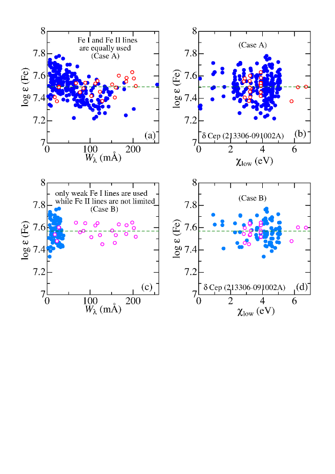
Figure 1: Line-by-line Fe abundances (corresponding to the finally established atmospheric parameters), plotted against equivalent widths (left panels) and lower excitation potentials (right panels), for the case of $\delta$ Cep (213306-091002A; the first spectrum for this star). The upper two panels (a, b) are for Case (A) where lines of $w<200$ m$\rm\AA$ ($w$ is the reduced equivalent width: $w\equiv W_{\lambda}\cdot(5000/\lambda)$) were equally used for both Fe i and Fe ii lines, while the lower two panels (c, d) correspond to Case (B) where lines were screened with the criterion of $w<30$ m$\rm\AA$ (Fe i) and $w<200$ m$\rm\AA$ (Fe ii) (i.e., only weak Fe i lines were used). The results for Fe i and Fe ii lines are distinguished by filled and open symbols, respectively, and the average Fe abundance is indicated by the horizontal dashed line.

We first carried out some test calculations by using the spectrum of $\delta$ Cep (213306-091002A), in order to confirm the argument of Kovtyukh & Andrievsky (1999), who suggested that Fe ii lines of various strengths can be safely used, while the mean abundance from Fe i lines should be determined based on only weak lines (as the weak-line limit). Namely, the following two different cases were examined concerning the input data set of $W_{\lambda}$.
— Case (A):
The TGVIT program was applied without any specific constraint on the line strengths (i.e., all available Fe i and Fe ii lines satisfying $w\leq 200$ m$\rm\AA$). Then, the solutions of [$T_{\rm eff}$ (K), $\log g$ (cm s^-1), $\xi$ (km s^-1), and [Fe/H] (dex)] minimizing $D^{2}$ were obtained as [5694, 1.88, 3.56, and 0.00]. However, the abundances from Fe i and Fe ii lines corresponding to these parameters turned out appreciably $W_{\lambda}$-dependent in an opposite manner (i.e., Fe i $|$ Fe ii abundances tend to progressively decrease $|$ increase with an increase in $W_{\lambda}$) as shown in Fig. 1a, which is hardly acceptable.
— Case (B):
Next, we restricted Fe i lines to only those fairly weak ones satisfying the criterion of $w\leq 30$ m$\rm\AA$, while Fe ii lines are usually used as before, in analogy with treatment suggested by Kovtyukh & Andrievsky (1999). The resulting parameter solutions for this case were [5706, 2.19, 3.88, and +0.07]; the especially notable change compared to Case (A) is an increase of $\log g$ by $\sim$ 0.3 dex. The $\log\epsilon$ vs. $W_{\lambda}$ relation for this case is displayed in Fig. 1c, where we can satisfactorily confirm that the Fe abundances do not show any systematic dependence upon $W_{\lambda}$. Naturally, as recognized in the $\log\epsilon$ vs. $\chi_{\rm low}$ plots, the abundance scatter around the mean is appreciably smaller for Case (B) (Fig. 1d) in comparison with Case (A) (Fig. 1b).

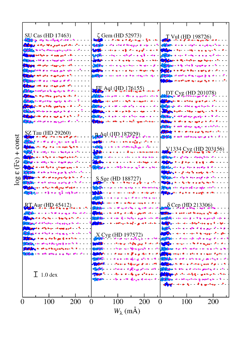
Figure 2: Fe abundance vs. equivalent width relations corresponding to the finally established atmospheric parameters of $T_{\rm eff}$, $\log g$, and $v_{\rm t}$ for each of the 122 spectra, being arranged according to the time sequence in the downward direction for each star (just as in Table 2). The filled and open symbols correspond to Fe i and Fe ii lines, respectively. The results for each stars are shown relative to the mean abundances indicated by the horizontal dotted lines, and vertically shifted by 1.0 relative to the adjacent ones.

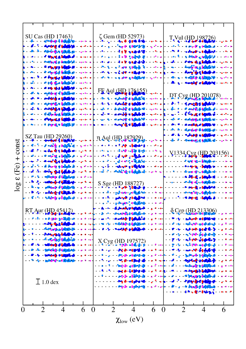
Figure 3: Fe abundance vs. lower excitation potential relation corresponding to the finally established atmospheric parameters for each of the 122 spectra. Otherwise, the same as in Fig. 2.

Given these results, which reconfirmed the consequence of Kovtyukh & Andrievsky (1999), we decided to follow Case (B) and use only the weak Fe i lines with $w\leq 30$ m$\rm\AA$ but all Fe ii lines with $w\leq 200$ m$\rm\AA$, as the input $W_{\lambda}$ data to which TGVIT was applied. The number of actually used Fe i lines after this screening was $\sim$ 40–130 (i.e., almost as half as the originally measured ones). The finally resulting parameters ($T_{\rm eff}$, $\log g$, $\xi$, and [Fe/H]) for each of the 122 spectra are presented in Table 2. The typical statistical uncertainties involved in these solutions estimated in the manner described in Section 3.2 of Takeda et al. (2002) are ($\sim 50$ K, $\sim 0.1$ dex, $\sim~{}0.3$ km s^-1, and $\sim~{}0.05$ dex), respectively. The corresponding $\log\epsilon$ vs. $W_{\lambda}$ and $\log\epsilon$ vs. $\chi_{\rm low}$ plots are depicted in Fig. 2 and Fig.3, respectively, where we can see that the requirements (a), (b), and (c) are reasonably fulfilled. The detailed line-by-line data ($W_{\lambda}$, $\log\epsilon$) for each stellar spectrum are also given as the electronic data tables contained in the supplementary materials (the results for HD ?????? are presented in the file named “??????_feabw.dat”).

4 Abundance Determinations

4.1 Target Lines of C, N, O, and Na

Regarding the choice of lines to be used for deriving the abundances of C, N, O, and Na, several requirements were taken into consideration:
— From the viewpoint of mutual consistency, lines of the same type had better be used for all these elements; so we would rely on permitted lines of neutral species.
— The strength of the line must not be too weak, so that firm detectability in the relevant parameter ranges ($T_{\rm eff}\sim$ 5000–7000 K, $\log g\sim$ 1–3) can be guaranteed.
— On the other hand, we would like to avoid considerably strong lines, such as those very sensitive to a non-LTE effect or microturbulence.
— Since our analysis is based on the spectrum synthesis method, it is preferable to select a wavelength region of moderate width comprising a few lines belonging the same multiplet, so that they may be analyzed at a time.

We then decided to invoke the following lines which reasonably meet these conditions: C i 7111/7113/7115/7116/7119 lines for C, N i 8680/8683/8686 lines for N, O i 6155–8 lines for O, and Na i 6154/6161 lines for Na.

4.2 Synthetic Spectrum Fitting

Abundance determinations in the first step were carried out by using our synthetic spectrum fitting code MPFIT, in which the spectrum synthesis part is originally based on Kurucz’s (1993) WIDTH9 program. It accomplishes the best-match between the theoretical and observational spectra based on the algorithm described in Takeda (1995), by simultaneously varying the abundances of several key elements ($\log\epsilon_{1}$, $\log\epsilon_{2}$, $\ldots$), macrobroadening parameter ($v_{\rm M}$), and the radial-velocity (wavelength) shift ($\Delta\lambda$). The macrobroadening parameter ($v_{\rm M}$) is the $e$-folding width of the Gaussian macrobroadening function, $M(v)\propto\exp[-(v/v_{\rm M})^{2}]$, which represents the combined effects of instrumental broadening, macroturbulence, and rotational velocity (though it is essentially dominated by mactroturbulence in the present case).

Practically, our spectrum fitting analysis was conducted for the following three wavelength regions, where the elements whose abundances were treated as variables are enumerated in each bracket: (i) 6143–6163 $\rm\AA$ [O, Na, Si, Ca, Fe] including O i 6155–8 and Na i 6154/6161 lines, (ii) 7110–7121 $\rm\AA$ [C, Fe, Ni] including C i 7111/7113/7115/7116/7119 lines and (iii) 8677–8697 $\rm\AA$ [N, Si, S, Fe] including N i 8680/8683/8686 lines.

Regarding the atomic data of spectral lines (wavelengths, excitation potentials, oscillator strengths, and damping constants), we basically invoked the compilation of Kurucz & Bell (1995). However, pre-adjustments of several $\log gf$ values were necessary (i.e., use of empirically determined solar $gf$ values) for several lines in 7110–7121 $\rm\AA$ region in order to accomplish a satisfactory match between the observed and theoretical spectrum. The finally adopted atomic data of important spectral lines are presented in table 2. The atmospheric model to be used for each spectrum was generated by interpolating Kurucz’s (1993) grid of ATLAS9 model atmospheres in terms of $T_{\rm eff}$, $\log g$, and [Fe/H].

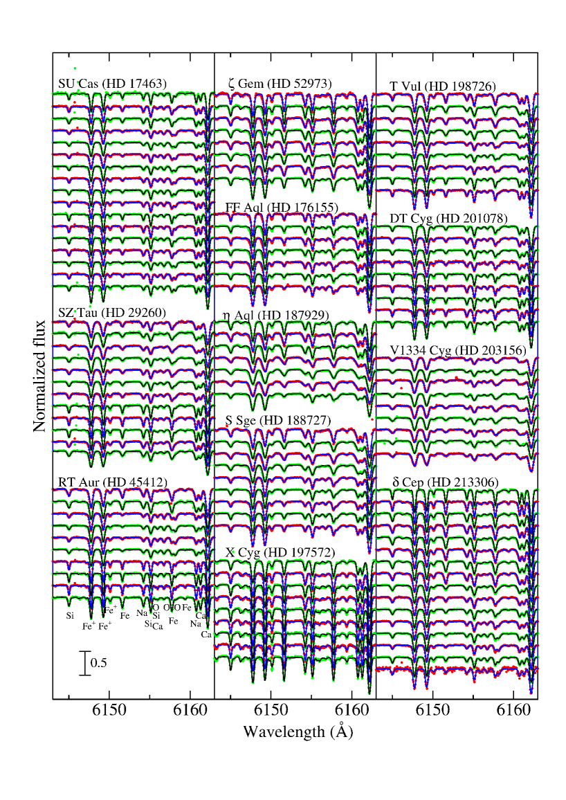
Figure 4: Synthetic spectrum fitting in the 6143–6163 $\rm\AA$ region accomplished by varying the abundances of O, Na, Si, Ca, and Fe, along with the macrobroadening velocity ($v_{\rm M}$) and the wavelength shift (radial velocity). The best-fit theoretical spectra are shown by solid lines, while the observed data are plotted by symbols, where the wavelength scale of the stellar spectrum has been adjusted to the laboratory frame. In each panel, the spectra are arranged according to the time sequence in the downward direction for each star (just as in Table 2), and each spectrum is vertically shifted by 0.25 relative to the adjacent one. The important lines (cf. Table 3) are identified in the lowest spectrum of the left panel.

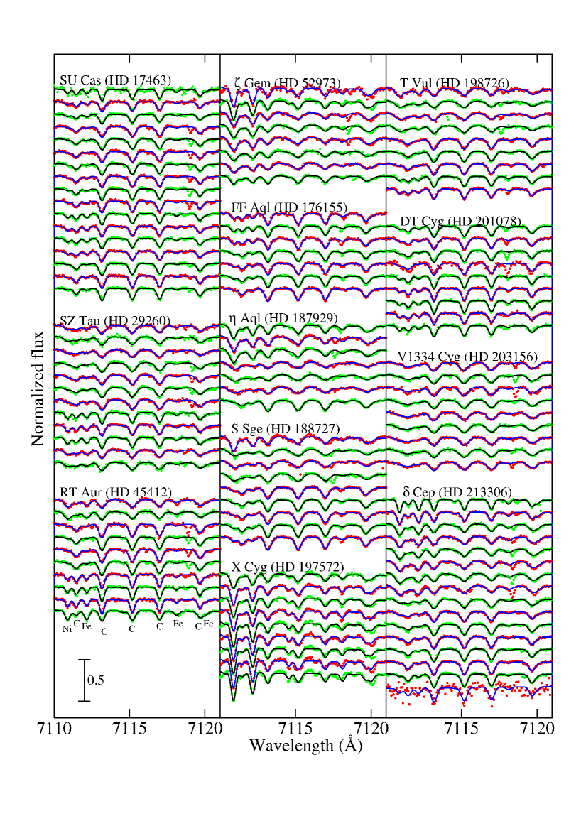
Figure 5: Synthetic spectrum fitting in the 7110–7121 $\rm\AA$ region accomplished by varying the abundances of C, Fe, and Ni. Each spectrum is vertically shifted by 0.15 relative to the adjacent one. Otherwise, the same as in Fig. 4.

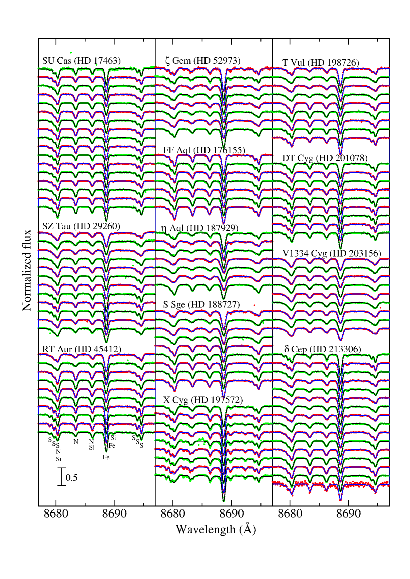
Figure 6: Synthetic spectrum fitting in the 8677–8697 $\rm\AA$ region accomplished by varying the abundances of N, Si, S, and Fe. Each spectrum is vertically shifted by 0.25 relative to the adjacent one. Otherwise, the same as in Fig. 4.

This fitting analysis turned out quite successful and we could obtain the abundances (especially for C, N, O, and Na) for all the 122 spectra. In case where some part of the spectrum was found to be damaged due to cosmic rays or telluric lines (e.g., occasionally encountered at $\lambda\sim 7118$ $\rm\AA$ in the 7110–7121 $\rm\AA$ fitting), such a region was masked and excluded from the evaluation of $\chi^{2}(O-C)$ evaluation. How the theoretical spectrum corresponding to the converged solutions fits well with the observed spectrum is displayed in figure 4 (6143–6163 $\rm\AA$ fitting), figure 5 (7110–7121 $\rm\AA$ fitting), and figure 6 (8677–8697 $\rm\AA$ fitting). Note that we assumed LTE for all lines at this stage of synthetic spectrum-fitting. The solutions of the macrobroadening width ($v_{\rm M}$) derived from the 6143–6163 $\rm\AA$ fitting are given in Table 2, while further work is yet to be done to establish the final abundances as described in the next Section 4.3.

4.3 Equivalent Widths Analysis

Despite that the synthetic spectrum fitting directly yielded the abundance solutions of C, N, O, and Na (the main purpose of this study), this approach is not necessarily suitable when one wants to examine how the results would be changed in different conditions (e.g., LTE vs. non-LTE, application of non-LTE calculations done at different assumptions, abundance sensitivity to parameter changes, etc.), since it is tedious to repeat the fitting process to obtain the new solution. Therefore, with the help of the modified version of Kurucz’s (1993) WIDTH9 program, we computed the equivalent widths for C i lines ($W_{7111}$, $W_{7113}$, $W_{7115}$, $W_{7116}$, $W_{7119}$), N i lines ($W_{8680}$, $W_{8683}$, $W_{8686}$), O i lines ($W_{6155-8}$), and Na i lines ($W_{6154}$, $W_{6161}$) “inversely” from the abundance solutions (resulting from spectrum synthesis) along with the adopted atmospheric model/parameters, which are much easier to handle. Based on such evaluated $W_{\lambda}$ values, the LTE ($\log\epsilon^{\rm LTE}$) as well as non-LTE abundances ($\log\epsilon^{\rm NLTE}$) were freshly computed, from which the non-LTE correction ($\Delta[\equiv\log\epsilon^{\rm NLTE}-\log\epsilon^{\rm LTE}$]) was further derived.

Regarding the calculations for evaluating the non-LTE departure coefficients, we followed the procedures described in Takeda & Takada-Hidai (2000) (for C), Takeda & Takada-Hidai (1995) (for N),Takeda & Takada-Hidai (1998) as well as Takeda et al. (2010) (for O), and Takeda & Takada-Hidai (1994) (for Na), which should be consulted for the details. In the actual non-LTE calculations for element X, two sets of departure coefficients were prepared corresponding to two different input theoretical abundances ([X/H]${}_{1}^{\rm t}$, [X/H]${}_{2}^{\rm t}$; expressed as the values relative to the solar abundance) which were so chosen as to encompass the real abundances of the program stars; i.e., ($-0.5$, 0.0) for C, (0.0, +1.0) for N, (0.0, $-0.5$) for O, and (0.0, +0.5) for Na. Then, from a given $W_{\lambda}$, we obtained two kinds of non-LTE abundances ($\log\epsilon_{1}$, $\log\epsilon_{2}$), which were further interpolated (or extrapolated) while requiring that the finally resulting non-LTE abundance be consistent with the input theoretical abundance (cf. Section 4.2 in Takeda & Takada-Hidai 1994).

The values of the equivalent width ($W_{i}$), non-LTE abundance ($\log\epsilon_{i}^{\rm NLTE}$), and non-LTE correction ($\Delta_{i}$) for each line $i$ of C, N, O, and Na, which were derived for all the 122 spectra, are presented as the electronic data tables (the results for HD ?????? are given in the file named “??????_cnona.dat”) contained in the supplementary materials.

The final non-LTE abundance and the non-LTE correction for element X, $\log\epsilon$(X) and $\Delta_{\rm X}$ (X = C, N, O, and Na), were eventually obtained by averaging $\log\epsilon_{i}^{\rm NLTE}$ and $\Delta_{i}$ over each relevant line $i$. We also calculated the differential abundance relative to the Sun as [X/H] $\equiv\log\epsilon$(X) $-$ $\log\epsilon_{\odot}$(X), which we will mainly use in the discussion. Regarding the reference solar abundances, we adopted the following values, which were derived from the solar flux spectra based on practically the same lines and the same atomic data by taking into account the non-LTE effect: $\log\epsilon_{\odot}$(C) = 8.51 (Takeda et al. 2013), $\log\epsilon_{\odot}$(N) = 8.05 (newly derived for this study from the N i 8683 line with the non-LTE correction of $-0.05$ dex, for which the solar $W_{8683}$ was measured to be 6.1 m$\rm\AA$), $\log\epsilon_{\odot}$(O) = 8.81 (Takeda & Honda 2005), and $\log\epsilon_{\odot}$(Na) = 6.32 (Takeda et al. 2003), where the abundance values are expressed in the usual normalization of $\log\epsilon$(H) = 12.00. The resulting [C/H], [N/H], [O/H], and [Na/H] (along with the corresponding $\Delta_{\rm C}$, $\Delta_{\rm N}$, $\Delta_{\rm O}$, and $\Delta_{\rm Na}$) derived for each of the 122 spectra are summarized in Table 2. As seen in this table, the extents of the (negative) non-LTE corrections are not significant for C, O, and Na ($\la 0.1$ dex), but rather considerable for N ($\sim$ 0.2–0.4 dex).

5 Discussion

5.1 Phase-Dependence of Physical Quantities

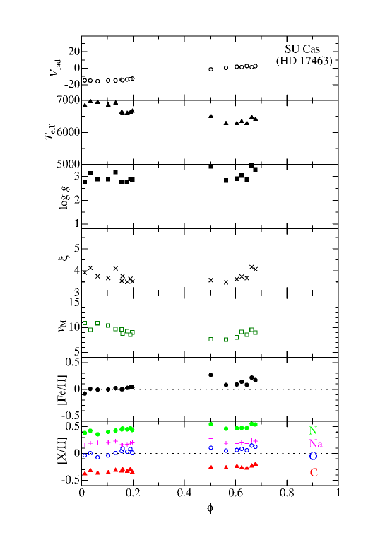
Figure 7: Results of the radial velocity, atmospheric parameters, and elemental abundances derived from each of the 17 spectra of SU Cas, plotted against the pulsation phase. Shown in these 7 panels are (from top to bottom): (a) heliocentric radial velocity (km s^-1), (b) effective temperature (K), (c) logarithmic surface gravity (cm s^-2), (d) microturbulence (km s^-1), (e) macrobroadening velocity (km s^-1), (f) [Fe/H] (dex), and (g) [X/H] (dex) where X is C (filled triangles), N (filled circles), O (open circles), and Na (greek crosses).

The results of the physical parameters in the atmosphere ($V_{\rm rad}$, $T_{\rm eff}$, $\log g$, $\xi$, $v_{\rm M}$) as well as the elemental abundances ([Fe/H], [C/H], [N/H], [O/H], and [Na/H]) are plotted against the phase ($\phi$) in Fig. 7–18 for each of the program stars (SU Cas, SZ Tau, RT Aur, $\zeta$ Gem, FF Aql, $\eta$ Aql, S Sge, X Cyg, T Vul, DT Cyg, V1334 Cyg, and $\delta$ Cep). Although we do not discuss these figures for each of the individual stars in detail, we can recognize several typical characteristics already known for Cepheid variables (see, e.g., Bersier, Burki & Kurucz 1997), such as the enhancement of $T_{\rm eff}$ and turbulent velocity fields ($\xi$ and $v_{\rm M}$ which are well-correlated) at the contraction or compressed phase of positive line-of-sight velocity (relative to the mean system velocity).

In order to check the results of our analysis, our values of $T_{\rm eff}$, $\log g$, $\xi$, and [Fe/H] derived for $\delta$ Cep (one of the best studied representative Cepheids) and those of previous studies (Luck & Lambert 1985; Kovtyukh, Komarov & Depenchuk 1994; Fry & Carney 1997; Kovtyukh & Andrievsky 1999; Andrievsky, Luck & Kovtyukh 2005) are overplotted against $\phi$ in Fig. 19, where we restricted the comparison to spectroscopically determined parameters derived in a similar manner to ours. We can see several notable trends from this figure:
— A remarkably good agreement with these literature values is seen for $T_{\rm eff}$ (Fig. 19a) and [Fe/H] (Fig. 19d).
— Our spectroscopic gravities are almost consistent with Kovtyukh & Andrievsky’s (1999) “non-standard” results, reflecting that both were derived in the same manner (mainly based on Fe ii lines along with the limited use of only very weak Fe i lines ), while older results using stronger Fe i lines (e.g., Fry & Carney 1997) tend to be appreciably lower by $\sim 0.5$ dex (Fig. 19b). This confirms the argument of Kovtyukh & Andrievsky (1999) that the spectroscopic $\log g$ based on the new “non-stadard” approach are preferable, since those old spectroscopic $\log g$ values of Cepheids (conventionally determined) were often found to be significantly lower than the dynamical values determined from the empirically estimated mass and radius (see, e.g., Luck & Lambert 1985).
— Regarding the microturbulence, our $\xi$ values tend to be systematically higher by $\sim 1$ km s^-1 in comparison with other literature results (Fig. 19c). The reason for this discrepancy is not clear, since it is observed not only in comparison with older work (where Fe i lines were used to determine $\xi$) but also with the non-standard results of Kovtyukh & Andrievsky (1999) (where $\xi$ was determined by Fe ii lines as in this study).

5.2 Correlation with Pulsation Period

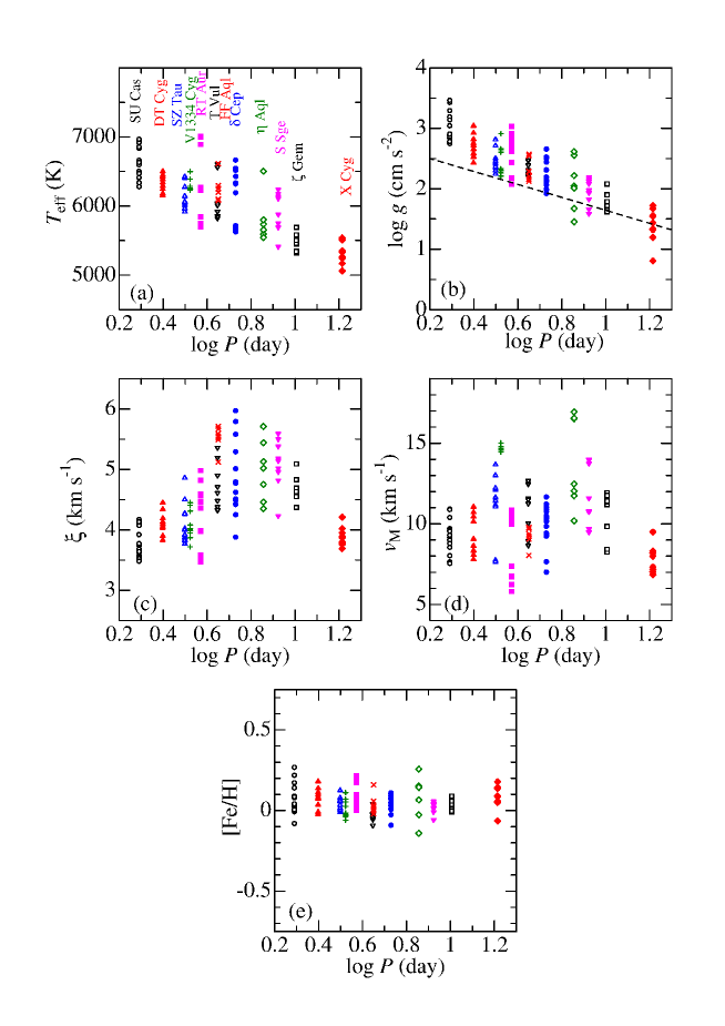
Figure 20: Atmospheric parameters derived from each of the 122 spectra, plotted against the pulsation period ($\log P$): (a) effective temperature, (b) logarithmic surface gravity, (c) microturbulence, (d) macrobroadening velocity, and (e) [Fe/H]. In panel (b), an approximate relation for dynamical $\log g$ given by equation (8) is also depicted by a dashed line. The results for each star are distinguished by the symbol type: SU Cas — open circles, DT Cyg — filled triangles, SZ Tau — open triangles, V1334 Cyg — Greek crosses (+), RT Aur — filled squares, T Vul — open downward triangles, FF Aql — St. Andrew’s crosses ($\times$), $\delta$ Cep — filled circles, $\eta$ Aql — open diamonds, S Sge — filled downward triangles, $\zeta$ Gem — open squares, X Cyg — filled diamonds.

Given that our program stars were so chosen as to cover a wide range of pulsation periods ($P\sim$ 2–16 days), it is worth examining how our spectroscopically determined atmospheric parameters depend on $P$, which is closely correlated with the absolute magnitude (also with the stellar mass) through the period–luminosity relation. Fig. 20 shows all the results of $T_{\rm eff}$, $\log g$, $\xi$, $v_{\rm M}$, and [Fe/H] derived for each of the 12 stars, plotted against $\log P$.

We can see a clear trend of $T_{\rm eff}$ decreasing with an increase in $\log P$ (Fig. 20a), which can be roughly represented by the linear relation

$$\log T_{\rm eff}=3.84-0.10\log P$$ (2)

($T_{\rm eff}$ is in K and $P$ is in days) with an uncertainty of a few hundred K. This reflects the fact the Cepheid instability strip is tilted in the theoretical $\log L$ vs. $\log T_{\rm eff}$ diagram, in the sense that higher-$L$ Cepheids with longer $P$ tend to have lower $T_{\rm eff}$.

We then discuss the $P$-dependence of $\log g$ (Fig. 20b). The surface gravity is expressed in terms of $M$, $L$, and $T_{\rm eff}$ as

$$\log(g/g_{\odot})=\log(M/M_{\odot})-\log(L/L_{\odot})+4\log(T_{\rm eff}/T_{\rm eff,\odot}).$$ (3)

If we use Benedict et al.’s (2007) period–luminosity relation for galactic Cepheids (cf. their fig. 5)

$$M_{V}=-1.62-2.43\log P$$ (4)

we have

$$\log(L/L_{\odot})=2.54-0.4B.C.+0.97\log P,$$ (5)

where $B.C.$ is the bolometric correction. We then invoke Caputo et al.’s (2005) mass–luminosity relation for solar composition (cf. their eq. (2))

$$\log(L/L_{\odot})=0.72+3.35\log(M/M_{\odot}).$$ (6)

Combining Eq. (5) and (6), we get a mass–period relation as

$$\log(M/M_{\odot})=0.54-0.12B.C.+0.29\log P.$$ (7)

Consequently, inserting Eq. (2), (5), and (7) into Eq. (3), we finally obtain

$$\log g=2.75+0.28B.C.-1.08\log P\simeq 2.72-1.08\log P$$ (8)

as the $P$-dependence of dynamical $\log g$, where we assumed $B.C.\simeq-0.1$ (actual values range from $\sim-0.2$ to $\sim 0.0$ depending on $T_{\rm eff}$, but insignificant; e.g., Flower 1996). This relation is also depicted in Fig. 20b. As seen from this figure, the spectroscopic $\log g$ values derived in this study tend to be systematically larger by this relation of dynamical $\log g$, which indicates that some of the relations we assumed above may not be appropriate or some systematic error may be involved in our $\log g$. Nevertheless, considering the large dispersion of observed $\log g$ along with the incomplete phase coverage of our data, we may regard that both are in tolerable consistency, despite the discrepancy especially in short-period Cepheids of $P\sim$ 2–3 days.

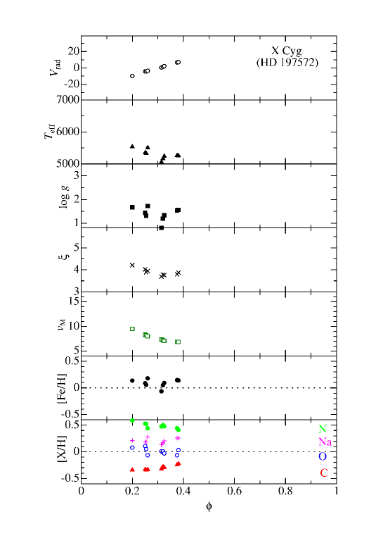
Figure 14: Results of the radial velocity, atmospheric parameters, and elemental abundances derived from each of the 9 spectra of X Cyg, plotted against the pulsation phase. Otherwise, the same as in Fig. 7.

Fig. 20c and 20d suggest that $\xi$ as well as $v_{\rm M}$ attain an apparent maximum at $\log P\sim 0.8$ and turn to decrease with increasing $P$, which may contradict the intuitive expectation that the atmospheric turbulence would progressively grow with a decrease of $\log g$ because of increased instability in lower-density condition. We consider, however, that this should not be taken too seriously, since the phase coverage of X Cyg (having the longest $P$ of 16 days) is insufficient and our 9 spectra for this star correspond to the expanding and decelerating phase ($\phi$ 0.2–0.4) of non-enhanced turbulence (Fig. 14).

The dispersion of [Fe/H] for each star in Fig. 20e suggests that the precision of its determination for a spectrum at a given phase (as a by-product of atmospheric parameter determination based on Fe i and Fe ii lines) is on the order of $\sim 0.1$ dex, though with rather large star-to-star differences (e.g., the reason for the appreciably larger [Fe/H] dispersion in S Sge is because our data correspond to $\phi\sim$ 0.7–1.1, where the spectral variation is rapid and the analysis is comparatively more difficult). Overall, these [Fe/H] values scatter around $\sim 0$ without any systematic dependence of [Fe/H] upon $P$, which means that all the program stars have almost the solar metallicity irrespective of the absolute magnitude and the mass.

Somewhat unexpectedly, such $P$-independent chemical homogeneity (i.e., small star-to-star abundance dispersion) was found also for the other elements. By averaging the [X/H]_i results for each individual spectrum $i$, we computed the mean abundance $\langle$[X/H]$\rangle$ and the standard deviation $\sigma_{\rm X}$ for each of the 12 stars (X = C, N, O, Na, and Fe), which are given in Table 2 (expressed in italic at the first line of each star’s section). These $\langle$[C/H]$\rangle$, $\langle$[N/H]$\rangle$, $\langle$[O/H]$\rangle$, $\langle$[Na/H]$\rangle$, and $\langle$[Fe/H]$\rangle$ for each star are plotted against $\log P$ in Fig. 21a–e, where the extents of relevant $\pm\sigma$ are shown as error bars. These figures demonstrate that none of these $\langle$[X/H]$\rangle$s show any significant $P$-dependence, which are practically homogeneous within a dispersion of $\la$ 0.1–0.2 dex. We may thus conclude $\langle$[C/H]$\rangle$ $\sim-0.3$, $\langle$[N/H]$\rangle$ $\sim$ +0.3–0.4, $\langle$[O/H]$\rangle$ $\sim 0$, $\langle$[Na/H]$\rangle$ $\sim+0.2$, and $\langle$[Fe/H]$\rangle$ $\sim 0$ as the abundance characteristics for these elements, which hold for all the program stars regardless of $\log P$. We note that these values are almost consistent with the recent extensive studies for various Cepheid variables (Andrievsky et al. 2005; Luck & Andrievsky 2004; Kovtyukh et al. 2005a; Luck et al. 2008), where we can see that their C, N, O, and Na abundances are almost the $P$-independent with the means (and the standard deviations) of $\langle$[C/H]$\rangle=-0.15$ ($\sigma=0.08$; 38 stars excluding SV Mon showing an exceptionally large deficiency of $-0.90$), $\langle$[N/H]$\rangle=+0.38$ ($\sigma=0.17$; 6 stars), $\langle$[O/H]$\rangle=-0.08$ ($\sigma=0.09$; 38 stars), and $\langle$[Na/H]$\rangle=+0.21$ ($\sigma=0.07$; 39 stars).

5.3 Abundance Trends and Their Implications

Now, since the abundances of key elements have been established, we can discuss the main problem which motivated this investigation (cf. Section 1): the nature of envelope mixing inferred from the characteristics of C, N, O, and Na abundances.

According to the results derived in Section 5.2, C is mildly deficient by $\sim 0.3$ dex, N is appreciably enhanced by $\sim$ 0.3–0.4 dex, Na is moderately overabundant by $\sim 0.2$ dex, while O (as well as Fe) is practically solar without any significant peculiarity (within an uncertainty of $\sim$ 0.1 dex). This tendency can be visually confirmed in Fig. 22a and Fig. 22b, where $\langle$[N/H]$\rangle$ vs. $\langle$[C/H]$\rangle$ and $\langle$[Na/H]$\rangle$ vs. $\langle$[O/H]$\rangle$ correlations are plotted, respectively.

Regarding the oxygen problem to be clarified in the first place, we can confidently state that any significant mixing of ON-cycle product has not taken place in the envelope of Cepheid variables. This means that the result of apparently subsolar [O/H] derived by Luck & Lambert (1985) is most likely due to the use of inappropriate atmospheric parameters (especially too low $\log g$), as suggested by Kovtyukh & Andrievsky (1999). Then, the abundance peculiarities of C and N must have been caused mainly by the dredge-up of CN-cycle product. The weak anti-correlation between the C and N abundances implied from Fig. 22a is qualitatively consistent with this scenario.

In order to check this quantitatively, the CNO abundances ($\log\epsilon$) of our program stars are plotted in the $\langle\log\epsilon$(N)$\rangle$ vs. $\langle\log\epsilon$(C+O)$\rangle$ diagram and the $\langle\log\epsilon$(N)$\rangle$ vs. $\langle\log\epsilon$(C)$\rangle$ diagram in Fig. 22c and Fig. 22d, respectively, where the expected relations under the condition that $\epsilon$(C+N+O) is conserved are also drawn. Further, the resulting sums of $\log\epsilon$(C+N+O) evaluated for the program stars are plotted against $\log P$ in Fig. 22e. We can confirm that the observed abundances are almost on the expected curve in Fig. 22c (compare this figure with Fig. 1 of Luck & Lambert 1985), and that $\log\epsilon$(C+N+O) is almost conserved at the solar value (Fig. 22f).

It should be remarked, however, that we can not rule out the possibility of only a slight underabundance in O caused by the dredge-up of some (not significant) ON-cycle product. Actually, Fig. 22d implies that $\log\epsilon$(N) vs. $\log\epsilon$(C) correlation can not necessarily be well described only by the conservation conditions of $\log\epsilon$(C+N) = $\log\epsilon_{\odot}$(C+N) and $\log\epsilon$(O) = $\log\epsilon_{\odot}$(O) for stars of $\log\epsilon$(N)$\ga 8.5$. Rather, it is more reasonable to consider that a mixing of some ON-cycled material could have caused a slight O-deficiency by several hundredths dex (within $\la 0.1$ dex) in order to explain the $\log\epsilon$(N) values of these stars (Fig. 22d).

Finally, our results of moderate enhancement of Na by $\sim 0.2$ dex indicate that the NeNa-cycle product is dredged-up in the envelope of Cepheid variables. Takeda & Takada-Hidai (1994) derived [Na/H] = +0.15 ($\eta$ Aql) and [Na/H] = $-0.07$ ($\zeta$ Gem) based on their non-LTE analysis of the Na i 8194.12 line. Comparing these with the present results of +0.16 ($\eta$ Aql) and +0.23 ($\zeta$ Gem), we can see an appreciable discrepancy for the latter. However, their old analysis should be regarded as less reliable, where the atmospheric parameters corresponding to the observed phase were not properly determined but roughly assumed while consulting the literature values.

5.4 Mass-Independent Mixing in Cepheids

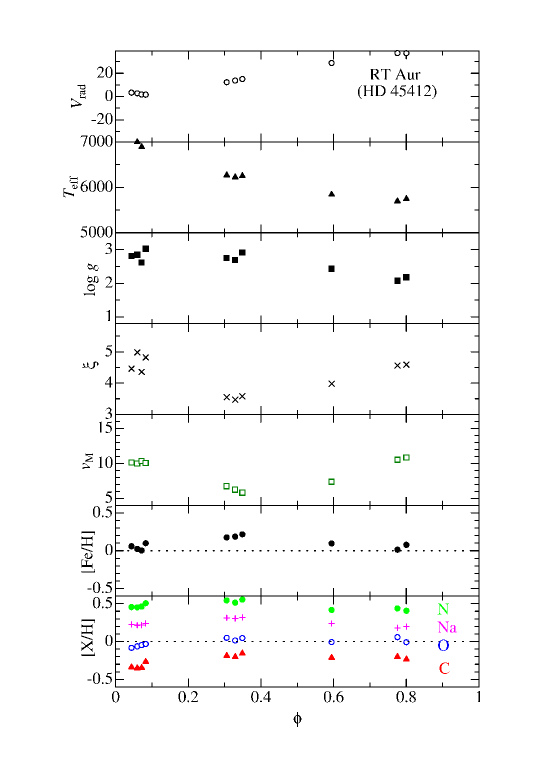
Figure 9: Results of the radial velocity, atmospheric parameters, and elemental abundances derived from each of the 10 spectra of RT Aur, plotted against the pulsation phase. Otherwise, the same as in Fig. 7.

Before starting this investigation, we anticipated that a significantly large abundance scatter may be found at least for C and N (or possibly also for O), as reported in the pioneering work by Luck & Lambert (1985; cf. Fig. 1 or Fig. 9 therein), and that such a diversity (if exists) might be correlated with $P$ (or equivalently, the stellar mass $M$). However, the considerably small star-to-star dispersion in the abundances of all elements (C, N, O, Na, Fe) was rather an unexpected result. Though, admittedly, a weak anti-correlation between N and C abundances (Fig. 22a, Fig. 22d) suggests that the extent of dredged-up material mixed in envelope may differ slightly from star to star, it does not appear to have anything to do with $M$, since [N/C] does not show any systematic dependence upon $P$ (Fig. 22e). So, another important outcome of this study is the confirmation that the extent of mixing in the envelope of Cepheid variables does not depend upon the stellar mass. Interestingly, essentially the same conclusion was reached by Kovtyukh, Wallerstein & Andrievsky (2005b), who carried out an extensive spectroscopic abundance study for 16 distant Cepheids with a wide range of $P$ ($\sim$ 3–27 days) and found that neither [C/N] ($\sim+0.6$) nor [Na/Fe] ($\sim+0.2$) show any systematic dependence upon $\log P$, which is quite consistent with our results.

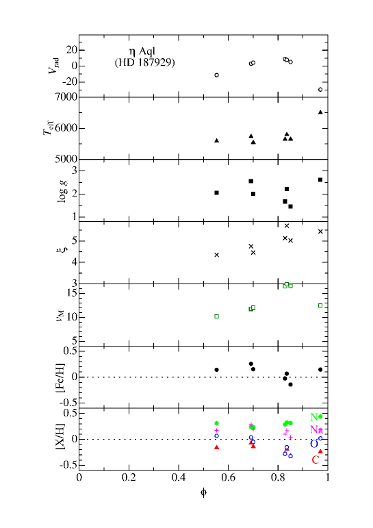
Figure 12: Results of the radial velocity, atmospheric parameters, and elemental abundances derived from each of the 7 spectra of $\eta$ Aql, plotted against the pulsation phase. Otherwise, the same as in Fig. 7.

We should note, however, that this consequence is guaranteed only for the pulsation variables within the Cepheid instability strip, which should not be simply extended to non-variable supergiants or giants in different parameter ranges (e.g., in terms of $T_{\rm eff}$ or $M$). For example, we can not say much about the argument of Takeda & Takada-Hidai (1994) (Na tends to be more enriched with an increase of mass for supergiants of $\sim$ 10–25 $M_{\odot}$; cf. Fig. 7 therein), since the mass range of the program stars in this study is between $\sim 4M_{\odot}$ and $\sim 8M_{\odot}$ according to Eq. (7), and their sample was mostly non-variable supergiants. Similarly, the systematic $\log g$-dependence of [Na/H] concluded by Andrievsky et al. (2002) was mainly due to supergiants (not Cepheids) of $0.5\la\log g\la 2$ (cf. their fig. 1), which is again less relevant to this study. Besides, Smiljanic et al. (2006) concluded based on their CNO abundance study for 19 non-variable supergiants covering a rather large range of stellar parameters (4100 K $\la T_{\rm eff}\la$ 7500 K, 0.8 $\la\log g\la$ 2.5, 2 $\la M/M_{\odot}\la$ 13) that the [N/C] ratios tend to increase with $M$ and have considerably larger values (up to $\la+2$) than the theoretical expectation. Further, Takeda, Sato & Murata (2008) reported in their analysis of 322 late-G and early-K giants (4500 K $\la T_{\rm eff}\la$ 5500 K, 1.5 $\la\log g\la$ 3.5, 1 $\la M/M_{\odot}\la$ 5) that [C/Fe], [O/Fe], and [Na/Fe] show subsolar, subsolar, and supersolar tendency, respectively, with the degree of peculiarity increasing with $M$ (cf. Fig. 12 therein), which may imply that a mass-dependent dredge-up of CN-cycle, ON-cycle, and NeNa-cycle products may take place in the envelope of red giants.

Consequently, we would still consider it quite possible that the mixing-induced abundance peculiarities of non-variable intermediate-mass evolved stars in general are significantly diversified and may depend on $M$. If so, we would have to find a reasonable answer to the question “Why the absence of large star-to-star dispersion or of $M$-dependence in the evolution-induced mixing is limited only to Cepheid variables?”, to which contributions by theoreticians are desirably awaited.

6 Conclusion

The mixing in the envelope of intermediate-mass F–G supergiants causing surface abundance peculiarities by the dredge-up of H-burning products is not yet well understood. Especially, regarding oxygen, whether or not its anomaly exists due to non-canonical dredge-up of ON-cycled material is still controversial.

In order to clarify this situation, we conducted an extensive spectroscopic study for selected 12 Cepheid variables of various pulsation periods ($\sim$ 2–16 days), and determined the photospheric abundances of C, N, O, and Na, which are the key elements for investigating the dredge-up of H-burning products from the interior, based on 122 high-dispersion spectra ($\sim 10$ spectra of different phases per target) of wide wavelength coverage collected at Bohyunsan Astronomical Observatory.

The atmospheric parameters ($T_{\rm eff}$, $\log g$, $\xi$, and [Fe/H]) corresponding to each phase were determined spectroscopically from the equivalent widths of Fe i and Fe ii lines by the requirements of excitation equilibrium, ionization equilibrium, and curve-of-growth matching. Practically, we applied Takeda et al.’s (2005) TGVIT program, while using only fairly weak Fe ilines ($\la 30$ m$\rm\AA$) as suggested by Kovtyukh & Andrievsky (1999) to avoid non-LTE-sensitive stronger Fe i lines. The resulting parameters as well as the radial velocities were confirmed to show the well-known phase-dependent characteristics of Cepheids.

The abundances of C, N, O, and Na were derived by applying the spectrum-synthesis fitting technique to three wavelength regions (6143–6163 $\rm\AA$, 7110–7121 $\rm\AA$, and 8677–8697 $\rm\AA$) comprising C i 7111/7113/7115/7116/7119, O i 6155–8, N i 8680/8683/8686, and Na i 6154/6161 lines. Then, from the equivalent widths inversely computed from the fitting-based abundances, the final abundances were obtained by taking into account the non-LTE effect.

The resulting abundances of these elements for 12 program stars turned out to show remarkably small star-to-star dispersions ($\la$ 0.1–0.2 dex) without any significant dependence upon the pulsation period: near-solar Fe ([Fe/H] $\sim 0.0$), moderately underabundant C ([C/H] $\sim-0.3$), appreciably overabundant N ([N/H] $\sim$ +0.4–0.5), and mildly supersolar Na ([Na/H] $\sim+0.2$). Based on these results, we conclude as follows.
— (1) These CNO abundance trends can be interpreted mainly as due to the canonical dredge-up of CN-cycled material, while the significant non-canonical deep mixing of ON-cycled gas is ruled out (though only a slight mixing may still be possible).
— (2) The mild but definite overabundance of Na suggests that the NeNa-cycle product is also dredged up.
— (3) The extent of mixing-induced peculiarities in the envelope of Cepheid variables is almost independent on $M_{V}$ as well as on $M$. However, given the observational suggestion that a significant diversity or a tendency of $M$-dependence exists in the C, N, O, and Na abundances of non-variable supergiants/giants of other types, the problem of “why such a homogeneity in the surface abundances is limited only to Cepheids” is yet to be investigated further.

Table 1: Basic data of the program stars.

Name	HD#	$\alpha_{2000}$	$\delta_{2000}$	Cep.Type	Sp.Type	$V$	Epoch	$P$
(1)	(2)	(3)	(4)	(5)	(6)	(7)	(8)	(9)
SU Cas	017463	02:51:58.8	+68:53:19	s	F5Ib/II–F7Ib/II	5.70–6.18	50100.156	1.949319
SZ Tau	029260	04:37:14.8	+18:32:35	s	F5Ib–F9.5Ib	6.33–6.75	50101.605	3.14873
RT Aur	045412	06:28:34.1	+30:29:35	cl	F4Ib–G1Ib	5.00–5.82	50101.159	3.728115
$\zeta$ Gem	052973	07:04:06.5	+20:34:13	cl	F7Ib–G3Ib	3.62–4.18	50108.93	10.15073
FF Aql	176155	18:58:14.7	+17:21:39	s	F5Ia–F8Ia	5.18–5.68	50102.387	4.470916
$\eta$ Aql	187929	19:52:28.4	+01:00:20	cl	F6Ib–G4Ib	3.48–4.39	50100.861	7.176641
S Sge	188727	19:56:01.3	+16:38:05	cl	F6Ib–G5Ib	5.24–6.04	50105.348	8.382086
X Cyg	197572	20:43:24.2	+35:35:16	cl	F7Ib–G8Ib	5.85–6.91	50106.014	16.386332
T Vul	198726	20:51:28.2	+28:15:02	cl	F5Ib–G0Ib	5.41–6.09	50101.410	4.435462
DT Cyg	201078	21:06:30.2	+31:11:05	s	F5.5–F7Ib/II	5.57–5.96	50102.487	2.499215
V1334 Cyg	203156	21:19:22.2	+38:14:15	s	F2Ib	5.77–5.96	50102.549	3.332816
$\delta$ Cep	213306	22:29:10.3	+58:24:55	cl	F5Ib–G1Ib	3.48–4.37	50102.860	5.366341

Following the star name and HD number (serial number in the Henry–Draper catalog) in Columns (1) and (2), the data of star coordinates (right ascension in HH:MM:SS.S and declination in deg:arcmin:arcsec), Cepheid type (“cl” for classical Cepheids and “s” for s-Cepheids), spectral type, and apparent visual magnitude (in mag) are presented in Columns (3)–(7), which were taken from the web site of General Catalogue of Variable Stars (http://www.sai.msu.su/gcvs/gcvs/index.htm). The last two Columns (8) and (9) give the epoch of brightness maximum expressed in Julian day (JD $-2400000$) and the pulsation period (in day), for which we consulted Table 1 of Kiss (1998).

Table 2: Results of stellar parameters and abundances derived from each spectrum of different phase.

Code	JD	$\phi$	$V_{\rm rad}$	$T_{\rm eff}$	$\log g$	[Fe]	$\xi$	$v_{\rm M}$	[C]	$\Delta_{\rm C}$	[N]	$\Delta_{\rm N}$	[O]	$\Delta_{\rm O}$	[Na]	$\Delta_{\rm Na}$
(1)	(2)	(3)	(4)	(5)	(6)	(7)	(8)	(9)	(10)	(11)	(12)	(13)	(14)	(15)	(16)	(17)
SU Cas (HD 017463)						${\it+0.06(\pm 0.09)}$			${\it-0.30(\pm 0.05)}$		${\it+0.46(\pm 0.05)}$		${\it+0.05(\pm 0.06)}$		${\it+0.20(\pm 0.03)}$
017463-091002A	6.99	0.503	$-$1.4	6500	3.43	+0.27	3.6	7.6	$-$0.26	$-$0.04	+0.55	$-$0.26	+0.11	$-$0.03	+0.28	$-$0.07
017463-091002B	7.22	0.623	+1.3	6336	3.04	+0.14	3.7	9.1	$-$0.27	$-$0.05	+0.48	$-$0.27	+0.09	$-$0.03	+0.21	$-$0.07
017463-091002C	7.30	0.663	+1.3	6469	3.46	+0.22	4.2	9.6	$-$0.23	$-$0.04	+0.55	$-$0.24	+0.15	$-$0.03	+0.25	$-$0.07
017463-091003A	7.98	0.012	$-$14.8	6833	2.76	$-$0.08	3.9	10.9	$-$0.38	$-$0.07	+0.38	$-$0.41	$-$0.03	$-$0.05	+0.16	$-$0.07
017463-091003B	8.08	0.062	$-$15.8	6935	2.88	$-$0.01	3.8	10.9	$-$0.37	$-$0.07	+0.36	$-$0.41	$-$0.07	$-$0.05	+0.20	$-$0.07
017463-091003C	8.16	0.103	$-$14.9	6853	2.89	+0.00	3.7	10.4	$-$0.36	$-$0.07	+0.40	$-$0.41	$-$0.04	$-$0.05	+0.21	$-$0.07
017463-091003D	8.21	0.132	$-$15.0	6916	3.19	+0.02	4.1	9.7	$-$0.31	$-$0.06	+0.43	$-$0.36	+0.01	$-$0.04	+0.23	$-$0.07
017463-091003E	8.26	0.156	$-$14.0	6632	2.75	+0.00	3.5	9.6	$-$0.33	$-$0.07	+0.45	$-$0.39	+0.05	$-$0.05	+0.16	$-$0.07
017463-091003F	8.30	0.178	$-$13.6	6599	2.75	+0.03	3.5	9.3	$-$0.33	$-$0.07	+0.45	$-$0.39	+0.03	$-$0.05	+0.17	$-$0.07
017463-091003G	8.34	0.197	$-$12.7	6660	2.86	+0.04	3.5	9.0	$-$0.35	$-$0.07	+0.44	$-$0.38	+0.02	$-$0.05	+0.21	$-$0.07
017463-091004A	9.05	0.563	+0.3	6279	2.83	+0.08	3.5	7.5	$-$0.27	$-$0.06	+0.46	$-$0.30	+0.05	$-$0.04	+0.19	$-$0.07
017463-091004B	9.14	0.605	+1.7	6279	2.90	+0.09	3.6	8.0	$-$0.24	$-$0.06	+0.47	$-$0.28	+0.06	$-$0.04	+0.19	$-$0.07
017463-091004C	9.21	0.643	+2.6	6278	2.86	+0.08	3.7	8.5	$-$0.28	$-$0.06	+0.47	$-$0.29	+0.06	$-$0.04	+0.18	$-$0.07
017463-091004D	9.28	0.677	+2.6	6410	3.29	+0.17	4.1	9.0	$-$0.20	$-$0.04	+0.54	$-$0.25	+0.12	$-$0.03	+0.23	$-$0.07
017463-091005A	9.97	0.034	$-$15.0	6964	3.14	+0.01	4.1	9.5	$-$0.32	$-$0.06	+0.42	$-$0.38	+0.01	$-$0.04	+0.19	$-$0.07
017463-091005B	10.22	0.160	$-$14.6	6596	2.78	+0.00	3.8	8.8	$-$0.30	$-$0.07	+0.47	$-$0.38	+0.09	$-$0.05	+0.16	$-$0.07
017463-091005C	10.28	0.190	$-$13.3	6629	2.90	+0.04	3.6	8.5	$-$0.30	$-$0.07	+0.47	$-$0.37	+0.08	$-$0.05	+0.19	$-$0.07
SZ Tau (HD 029260)						${\it+0.05(\pm 0.04)}$			${\it-0.26(\pm 0.04)}$		${\it+0.48(\pm 0.05)}$		${\it+0.03(\pm 0.04)}$		${\it+0.22(\pm 0.03)}$
029260-091002A	7.15	0.704	+10.0	6010	2.42	+0.01	4.3	12.2	$-$0.24	$-$0.07	+0.54	$-$0.31	+0.07	$-$0.05	+0.18	$-$0.08
029260-091002B	7.24	0.732	+8.9	6143	2.71	+0.07	4.9	13.0	$-$0.22	$-$0.06	+0.57	$-$0.28	+0.11	$-$0.04	+0.22	$-$0.07
029260-091002C	7.32	0.758	+7.2	6141	2.42	$-$0.01	4.5	13.7	$-$0.29	$-$0.07	+0.46	$-$0.32	$-$0.01	$-$0.05	+0.18	$-$0.07
029260-091003A	8.17	0.027	$-$11.0	6405	2.41	+0.06	4.0	12.1	$-$0.31	$-$0.08	+0.41	$-$0.38	$-$0.03	$-$0.06	+0.25	$-$0.07
029260-091003B	8.23	0.045	$-$10.6	6272	2.24	+0.00	3.9	11.6	$-$0.29	$-$0.09	+0.46	$-$0.39	+0.01	$-$0.07	+0.21	$-$0.08
029260-091003C	8.27	0.059	$-$9.7	6276	2.35	+0.01	4.0	11.4	$-$0.25	$-$0.09	+0.48	$-$0.38	+0.04	$-$0.06	+0.21	$-$0.08
029260-091003D	8.32	0.073	$-$9.8	6427	2.81	+0.12	4.5	11.2	$-$0.17	$-$0.06	+0.53	$-$0.33	+0.07	$-$0.05	+0.28	$-$0.07
029260-091004A	9.15	0.337	$-$0.8	6044	2.50	+0.08	3.9	7.7	$-$0.25	$-$0.07	+0.45	$-$0.29	$-$0.04	$-$0.04	+0.25	$-$0.08
029260-091004B	9.22	0.362	+0.6	5968	2.46	+0.06	3.8	7.6	$-$0.20	$-$0.07	+0.47	$-$0.28	+0.02	$-$0.04	+0.23	$-$0.08
029260-091004C	9.29	0.384	+1.9	5919	2.30	+0.03	3.8	7.7	$-$0.26	$-$0.07	+0.47	$-$0.29	$-$0.01	$-$0.05	+0.21	$-$0.08
029260-091005A	10.15	0.655	+11.7	5961	2.35	+0.06	3.9	11.1	$-$0.26	$-$0.07	+0.46	$-$0.30	+0.01	$-$0.05	+0.21	$-$0.08
029260-091005B	10.30	0.704	+10.4	6063	2.36	+0.06	4.3	12.2	$-$0.32	$-$0.08	+0.42	$-$0.31	+0.05	$-$0.05	+0.21	$-$0.08
RT Aur (HD 045412)						${\it+0.09(\pm 0.07)}$			${\it-0.25(\pm 0.07)}$		${\it+0.47(\pm 0.05)}$		${\it-0.01(\pm 0.05)}$		${\it+0.25(\pm 0.05)}$
045412-091002A	7.18	0.776	+37.2	5695	2.08	+0.01	4.6	10.5	$-$0.20	$-$0.07	+0.44	$-$0.25	+0.06	$-$0.04	+0.18	$-$0.07
045412-091002B	7.27	0.800	+37.1	5746	2.18	+0.08	4.6	10.8	$-$0.23	$-$0.07	+0.41	$-$0.24	$-$0.01	$-$0.04	+0.20	$-$0.07
045412-091003A	8.18	0.043	+3.3	7001	2.81	+0.06	4.5	10.1	$-$0.34	$-$0.07	+0.45	$-$0.45	$-$0.08	$-$0.05	+0.23	$-$0.06
045412-091003B	8.24	0.060	+2.8	7000	2.85	+0.02	5.0	10.0	$-$0.35	$-$0.07	+0.45	$-$0.43	$-$0.06	$-$0.05	+0.22	$-$0.06
045412-091003C	8.29	0.072	+1.7	6890	2.61	+0.00	4.4	10.3	$-$0.35	$-$0.08	+0.46	$-$0.46	$-$0.05	$-$0.05	+0.22	$-$0.06
045412-091003D	8.33	0.083	+1.6	7005	3.03	+0.10	4.8	10.1	$-$0.27	$-$0.06	+0.51	$-$0.42	$-$0.03	$-$0.04	+0.24	$-$0.06
045412-091004A	9.16	0.306	+12.3	6269	2.75	+0.17	3.5	6.7	$-$0.19	$-$0.07	+0.54	$-$0.32	+0.05	$-$0.04	+0.31	$-$0.08
045412-091004B	9.25	0.329	+13.6	6223	2.69	+0.18	3.5	6.2	$-$0.20	$-$0.07	+0.51	$-$0.32	+0.01	$-$0.04	+0.30	$-$0.08
045412-091004C	9.32	0.349	+15.0	6250	2.92	+0.22	3.6	5.8	$-$0.16	$-$0.06	+0.55	$-$0.29	+0.04	$-$0.04	+0.32	$-$0.07
045412-091005A	10.24	0.595	+28.8	5843	2.43	+0.10	4.0	7.4	$-$0.21	$-$0.06	+0.42	$-$0.24	$-$0.01	$-$0.04	+0.24	$-$0.07
$\zeta$ Gem (HD 052973)						${\it+0.04(\pm 0.03)}$			${\it-0.29(\pm 0.10)}$		${\it+0.35(\pm 0.05)}$		${\it-0.14(\pm 0.11)}$		${\it+0.23(\pm 0.03)}$
052973-091002A	7.20	0.405	+17.5	5321	1.68	+0.05	4.4	8.2	$-$0.17	$-$0.07	+0.38	$-$0.19	$-$0.14	$-$0.03	+0.19	$-$0.07
052973-091002B	7.29	0.413	+18.3	5342	1.90	+0.06	4.4	8.4	$-$0.12	$-$0.06	+0.40	$-$0.18	+0.09	$-$0.03	+0.19	$-$0.07
052973-091003A	8.25	0.508	+22.6	5452	1.76	+0.02	4.7	11.2	$-$0.28	$-$0.07	+0.29	$-$0.20	$-$0.13	$-$0.04	+0.24	$-$0.07
052973-091003B	8.29	0.512	+22.6	5462	1.72	+0.04	4.6	11.3	$-$0.29	$-$0.08	+0.29	$-$0.21	$-$0.14	$-$0.04	+0.25	$-$0.07
052973-091003C	8.33	0.516	+22.5	5501	1.78	+0.06	4.5	11.4	$-$0.27	$-$0.08	+0.28	$-$0.22	$-$0.22	$-$0.04	+0.26	$-$0.07
052973-091004A	9.25	0.607	+17.5	5691	2.08	+0.09	5.1	11.9	$-$0.33	$-$0.07	+0.38	$-$0.23	$-$0.20	$-$0.04	+0.27	$-$0.07
052973-091004B	9.33	0.615	+16.9	5581	1.62	$-$0.01	4.6	11.8	$-$0.41	$-$0.09	+0.35	$-$0.26	$-$0.32	$-$0.05	+0.22	$-$0.07
052973-091005A	10.25	0.706	+5.8	5688	1.79	+0.00	4.8	9.8	$-$0.41	$-$0.09	+0.43	$-$0.28	$-$0.07	$-$0.05	+0.21	$-$0.07
FF Aql (HD 176155)						${\it+0.04(\pm 0.06)}$			${\it-0.34(\pm 0.03)}$		${\it+0.54(\pm 0.02)}$		${\it-0.06(\pm 0.02)}$		${\it+0.27(\pm 0.02)}$
176155-091002A	6.93	0.356	$-$18.8	6246	2.57	+0.16	5.1	8.0	$-$0.27	$-$0.07	+0.58	$-$0.33	$-$0.02	$-$0.05	+0.31	$-$0.07
176155-091003A	7.92	0.578	$-$9.7	6081	2.28	+0.02	5.5	9.1	$-$0.35	$-$0.08	+0.52	$-$0.32	$-$0.07	$-$0.05	+0.25	$-$0.07
176155-091003B	7.99	0.593	$-$9.7	6099	2.29	+0.03	5.5	9.2	$-$0.34	$-$0.08	+0.51	$-$0.32	$-$0.09	$-$0.05	+0.26	$-$0.07
176155-091004A	8.91	0.799	$-$13.8	6198	2.13	$-$0.02	5.7	9.8	$-$0.35	$-$0.09	+0.55	$-$0.38	$-$0.06	$-$0.06	+0.25	$-$0.07
176155-091004B	8.96	0.810	$-$13.9	6256	2.16	+0.01	5.5	9.8	$-$0.36	$-$0.09	+0.54	$-$0.39	$-$0.10	$-$0.06	+0.27	$-$0.07
176155-091004C	9.07	0.834	$-$16.5	6294	2.20	+0.00	5.6	9.7	$-$0.36	$-$0.09	+0.55	$-$0.39	$-$0.06	$-$0.06	+0.27	$-$0.07
176155-091005A	9.93	0.026	$-$25.6	6612	2.54	+0.06	5.7	9.4	$-$0.33	$-$0.07	+0.56	$-$0.40	$-$0.04	$-$0.05	+0.30	$-$0.06
$\eta$ Aql (HD 187929)						${\it+0.09(\pm 0.12)}$			${\it-0.20(\pm 0.08)}$		${\it+0.31(\pm 0.06)}$		${\it-0.10(\pm 0.14)}$		${\it+0.16(\pm 0.07)}$
187929-091002A	6.95	0.553	$-$11.4	5591	2.05	+0.14	4.3	10.2	$-$0.16	$-$0.07	+0.31	$-$0.22	+0.07	$-$0.04	+0.17	$-$0.07
187929-091003A	7.94	0.691	+3.0	5735	2.55	+0.26	4.8	11.7	$-$0.07	$-$0.05	+0.24	$-$0.18	+0.04	$-$0.03	+0.29	$-$0.07
187929-091003B	8.00	0.700	+4.3	5542	2.01	+0.15	4.5	12.0	$-$0.14	$-$0.07	+0.23	$-$0.20	$-$0.05	$-$0.04	+0.19	$-$0.07
187929-091004A	8.92	0.828	+8.9	5649	1.67	$-$0.03	5.1	16.5	$-$0.27	$-$0.09	+0.29	$-$0.26	$-$0.28	$-$0.05	+0.10	$-$0.07
187929-091004B	8.97	0.835	+7.8	5799	2.22	+0.07	5.7	16.9	$-$0.19	$-$0.07	+0.33	$-$0.23	$-$0.15	$-$0.04	+0.17	$-$0.07
187929-091004C	9.08	0.850	+5.1	5654	1.45	$-$0.14	5.0	16.6	$-$0.32	$-$0.11	+0.31	$-$0.29	$-$0.32	$-$0.05	+0.04	$-$0.07
187929-091005A	9.94	0.970	$-$29.4	6502	2.61	+0.14	5.4	12.5	$-$0.24	$-$0.07	+0.44	$-$0.34	+0.02	$-$0.05	+0.18	$-$0.07

Table 2: (Continued.)

Code	JD	$\phi$	$V_{\rm rad}$	$T_{\rm eff}$	$\log g$	[Fe]	$\xi$	$v_{\rm M}$	[C]	$\Delta_{\rm C}$	[N]	$\Delta_{\rm N}$	[O]	$\Delta_{\rm O}$	[Na]	$\Delta_{\rm Na}$
(1)	(2)	(3)	(4)	(5)	(6)	(7)	(8)	(9)	(10)	(11)	(12)	(13)	(14)	(15)	(16)	(17)
S Sge (HD 188727)						${\it+0.02(\pm 0.03)}$			${\it-0.25(\pm 0.03)}$		${\it+0.39(\pm 0.10)}$		${\it-0.10(\pm 0.16)}$		${\it+0.15(\pm 0.02)}$
188727-091002A	6.95	0.702	+22.3	5410	1.59	$-$0.01	4.2	11.6	$-$0.26	$-$0.08	+0.21	$-$0.20	$-$0.24	$-$0.04	+0.14	$-$0.07
188727-091003A	7.94	0.820	+20.0	5750	1.83	+0.04	5.2	14.0	$-$0.24	$-$0.09	+0.28	$-$0.26	$-$0.27	$-$0.05	+0.12	$-$0.07
188727-091003B	8.01	0.827	+18.4	5690	1.66	$-$0.06	5.5	14.0	$-$0.24	$-$0.10	+0.33	$-$0.27	$-$0.22	$-$0.05	+0.10	$-$0.07
188727-091003C	8.10	0.839	+15.3	5878	1.93	+0.04	5.6	13.7	$-$0.31	$-$0.09	+0.28	$-$0.28	$-$0.34	$-$0.05	+0.17	$-$0.07
188727-091004A	8.94	0.939	$-$9.3	6176	2.12	+0.01	5.4	10.8	$-$0.26	$-$0.09	+0.44	$-$0.36	+0.02	$-$0.07	+0.15	$-$0.07
188727-091004B	8.97	0.943	$-$10.4	6175	2.15	+0.04	5.1	10.8	$-$0.23	$-$0.09	+0.49	$-$0.36	+0.03	$-$0.07	+0.15	$-$0.07
188727-091004C	9.08	0.956	$-$12.1	6238	2.19	+0.04	5.0	10.7	$-$0.24	$-$0.09	+0.49	$-$0.37	+0.04	$-$0.07	+0.16	$-$0.07
188727-091005A	9.94	0.059	$-$12.9	6109	1.98	+0.02	5.0	9.7	$-$0.21	$-$0.10	+0.49	$-$0.38	+0.07	$-$0.08	+0.14	$-$0.08
188727-091005B	10.07	0.074	$-$12.2	6136	2.08	+0.06	4.8	9.5	$-$0.21	$-$0.10	+0.48	$-$0.37	+0.05	$-$0.07	+0.17	$-$0.07
X Cyg (HD 197572)						${\it+0.09(\pm 0.07)}$			${\it-0.30(\pm 0.04)}$		${\it+0.49(\pm 0.05)}$		${\it+0.01(\pm 0.06)}$		${\it+0.21(\pm 0.04)}$
197572-091002A	7.12	0.200	$-$10.0	5537	1.67	+0.14	4.2	9.5	$-$0.34	$-$0.08	+0.59	$-$0.29	+0.08	$-$0.06	+0.21	$-$0.07
197572-091003a	7.95	0.250	$-$4.2	5349	1.44	+0.09	4.0	8.3	$-$0.33	$-$0.09	+0.53	$-$0.24	+0.11	$-$0.05	+0.19	$-$0.07
197572-091003b	8.02	0.254	$-$4.3	5331	1.32	+0.06	3.9	8.2	$-$0.34	$-$0.09	+0.52	$-$0.25	+0.05	$-$0.05	+0.19	$-$0.07
197572-091003c	8.11	0.260	$-$3.5	5509	1.72	+0.18	4.0	8.0	$-$0.34	$-$0.08	+0.44	$-$0.25	$-$0.07	$-$0.05	+0.28	$-$0.07
197572-091004A	8.99	0.314	+0.6	5059	0.81	$-$0.07	3.7	7.3	$-$0.32	$-$0.10	+0.47	$-$0.22	+0.01	$-$0.05	+0.13	$-$0.05
197572-091004B	9.09	0.320	+1.4	5167	1.19	+0.05	3.8	7.2	$-$0.28	$-$0.09	+0.50	$-$0.21	+0.01	$-$0.04	+0.17	$-$0.06
197572-091004C	9.17	0.325	+2.2	5243	1.33	+0.09	3.8	7.0	$-$0.29	$-$0.09	+0.48	$-$0.22	$-$0.03	$-$0.04	+0.20	$-$0.07
197572-091005A	10.00	0.375	+6.7	5265	1.54	+0.14	3.8	6.8	$-$0.24	$-$0.08	+0.44	$-$0.20	$-$0.06	$-$0.04	+0.26	$-$0.07
197572-091005B	10.09	0.381	+7.0	5254	1.56	+0.14	3.9	6.8	$-$0.22	$-$0.08	+0.41	$-$0.19	+0.03	$-$0.04	+0.26	$-$0.07
T Vul (HD 198726)						${\it-0.03(\pm 0.03)}$			${\it-0.29(\pm 0.05)}$		${\it+0.35(\pm 0.07)}$		${\it-0.08(\pm 0.07)}$		${\it+0.09(\pm 0.02)}$
198726-091002A	6.96	0.530	+9.9	5821	2.46	+0.04	4.5	10.0	$-$0.22	$-$0.06	+0.34	$-$0.22	$-$0.06	$-$0.03	+0.10	$-$0.07
198726-091003A	7.96	0.754	+16.8	5854	2.23	$-$0.03	5.2	12.5	$-$0.29	$-$0.07	+0.24	$-$0.24	$-$0.15	$-$0.04	+0.12	$-$0.07
198726-091003B	8.03	0.770	+16.6	5847	2.25	$-$0.06	5.4	12.6	$-$0.24	$-$0.07	+0.28	$-$0.24	$-$0.10	$-$0.04	+0.09	$-$0.07
198726-091003C	8.12	0.792	+15.0	5917	2.20	$-$0.03	4.9	12.7	$-$0.33	$-$0.08	+0.27	$-$0.27	$-$0.23	$-$0.04	+0.09	$-$0.07
198726-091004A	8.95	0.979	$-$17.5	6558	2.39	$-$0.09	4.7	11.6	$-$0.35	$-$0.08	+0.37	$-$0.39	$-$0.04	$-$0.06	+0.07	$-$0.07
198726-091004B	9.00	0.990	$-$17.6	6605	2.48	$-$0.05	4.4	11.5	$-$0.33	$-$0.08	+0.38	$-$0.40	$-$0.07	$-$0.06	+0.08	$-$0.07
198726-091004C	9.10	0.013	$-$18.3	6562	2.48	$-$0.04	4.6	11.2	$-$0.33	$-$0.08	+0.39	$-$0.39	$-$0.04	$-$0.06	+0.10	$-$0.07
198726-091005A	9.98	0.211	$-$7.5	6036	2.38	$-$0.02	4.3	8.9	$-$0.22	$-$0.07	+0.46	$-$0.30	+0.02	$-$0.05	+0.07	$-$0.08
198726-091005B	10.10	0.237	$-$6.8	6010	2.31	$-$0.02	4.3	8.7	$-$0.28	$-$0.08	+0.39	$-$0.30	$-$0.02	$-$0.05	+0.06	$-$0.08
DT Cyg (HD 201078)						${\it+0.08(\pm 0.06)}$			${\it-0.19(\pm 0.05)}$		${\it+0.49(\pm 0.03)}$		${\it+0.05(\pm 0.02)}$		${\it+0.25(\pm 0.03)}$
201078-091003A	7.97	0.820	+2.6	6245	2.43	$-$0.02	4.1	10.1	$-$0.24	$-$0.08	+0.44	$-$0.34	+0.04	$-$0.06	+0.18	$-$0.07
201078-091003B	8.04	0.850	+1.0	6341	2.58	$-$0.01	4.3	10.4	$-$0.24	$-$0.07	+0.44	$-$0.34	+0.04	$-$0.05	+0.23	$-$0.07
201078-091003C	8.13	0.886	$-$0.5	6448	2.82	+0.10	4.2	10.7	$-$0.17	$-$0.07	+0.49	$-$0.33	+0.03	$-$0.05	+0.26	$-$0.07
201078-091003D	8.19	0.911	$-$2.0	6502	2.92	+0.14	4.5	11.1	$-$0.08	$-$0.06	+0.47	$-$0.32	+0.07	$-$0.05	+0.28	$-$0.07
201078-091004A	9.01	0.239	$-$4.7	6386	2.75	+0.11	3.9	8.3	$-$0.19	$-$0.07	+0.51	$-$0.34	+0.07	$-$0.05	+0.27	$-$0.07
201078-091004B	9.11	0.278	$-$3.5	6292	2.65	+0.08	3.8	8.1	$-$0.19	$-$0.07	+0.52	$-$0.34	+0.08	$-$0.05	+0.25	$-$0.07
201078-091004C	9.18	0.307	$-$3.0	6421	3.04	+0.18	4.0	7.8	$-$0.15	$-$0.06	+0.55	$-$0.30	+0.08	$-$0.04	+0.30	$-$0.07
201078-091005A	10.02	0.642	+5.2	6181	2.71	+0.07	4.1	8.6	$-$0.20	$-$0.06	+0.49	$-$0.29	+0.03	$-$0.04	+0.24	$-$0.07
201078-091005B	10.11	0.680	+5.0	6155	2.52	+0.04	4.0	9.1	$-$0.26	$-$0.07	+0.51	$-$0.32	+0.02	$-$0.05	+0.21	$-$0.07
V1334 Cyg (HD 203156)						${\it+0.01(\pm 0.06)}$			${\it-0.24(\pm 0.03)}$		${\it+0.44(\pm 0.03)}$		${\it+0.03(\pm 0.03)}$		${\it+0.11(\pm 0.04)}$
203156-091003A	8.06	0.886	$-$22.4	6286	2.20	$-$0.06	4.0	14.7	$-$0.26	$-$0.10	+0.48	$-$0.40	+0.05	$-$0.07	+0.03	$-$0.07
203156-091003B	8.14	0.911	$-$22.6	6496	2.60	+0.03	4.3	14.7	$-$0.26	$-$0.08	+0.46	$-$0.38	+0.04	$-$0.06	+0.13	$-$0.07
203156-091003C	8.20	0.927	$-$22.6	6503	2.65	+0.05	4.4	14.6	$-$0.28	$-$0.07	+0.45	$-$0.37	+0.07	$-$0.06	+0.12	$-$0.07
203156-091004A	8.93	0.145	$-$19.0	6260	2.33	$-$0.03	4.0	14.4	$-$0.23	$-$0.09	+0.43	$-$0.36	+0.04	$-$0.06	+0.09	$-$0.07
203156-091004B	9.03	0.176	$-$19.2	6231	2.21	$-$0.01	3.7	14.5	$-$0.25	$-$0.10	+0.42	$-$0.38	+0.00	$-$0.07	+0.09	$-$0.08
203156-091004C	9.12	0.204	$-$17.9	6388	2.66	+0.07	4.1	14.6	$-$0.20	$-$0.07	+0.45	$-$0.34	+0.02	$-$0.05	+0.15	$-$0.07
203156-091004D	9.19	0.226	$-$17.1	6246	2.30	$-$0.03	4.0	14.4	$-$0.27	$-$0.09	+0.43	$-$0.37	+0.01	$-$0.06	+0.10	$-$0.08
203156-091005A	10.04	0.479	$-$12.2	6249	2.26	$-$0.04	3.9	14.8	$-$0.22	$-$0.10	+0.39	$-$0.37	$-$0.03	$-$0.06	+0.08	$-$0.08
203156-091005C	10.18	0.523	$-$11.5	6499	2.91	+0.11	4.5	15.0	$-$0.18	$-$0.06	+0.47	$-$0.33	+0.04	$-$0.05	+0.18	$-$0.07
$\delta$ Cep (HD 213306)						${\it+0.04(\pm 0.05)}$			${\it-0.22(\pm 0.05)}$		${\it+0.39(\pm 0.07)}$		${\it+0.02(\pm 0.06)}$		${\it+0.17(\pm 0.04)}$
213306-091002A	6.98	0.502	$-$14.1	5706	2.19	+0.07	3.9	7.0	$-$0.23	$-$0.07	+0.40	$-$0.24	$-$0.01	$-$0.04	+0.15	$-$0.07
213306-091002B	7.22	0.545	$-$11.5	5713	2.31	+0.09	4.2	7.6	$-$0.18	$-$0.06	+0.41	$-$0.22	+0.04	$-$0.04	+0.17	$-$0.07
213306-091003A	7.98	0.687	$-$4.1	5682	2.06	+0.11	4.5	9.8	$-$0.24	$-$0.07	+0.29	$-$0.23	$-$0.03	$-$0.04	+0.21	$-$0.07
213306-091003B	8.07	0.705	$-$3.8	5661	2.12	+0.10	4.6	10.2	$-$0.20	$-$0.07	+0.33	$-$0.22	+0.02	$-$0.04	+0.19	$-$0.07
213306-091003C	8.15	0.720	$-$1.9	5666	2.14	+0.09	4.8	10.5	$-$0.17	$-$0.07	+0.34	$-$0.22	+0.03	$-$0.04	+0.18	$-$0.07
213306-091003D	8.21	0.730	$-$1.5	5625	1.98	+0.01	4.8	10.8	$-$0.18	$-$0.07	+0.33	$-$0.23	+0.04	$-$0.04	+0.17	$-$0.07
213306-091003E	8.26	0.739	$-$1.6	5633	1.92	+0.03	4.8	11.0	$-$0.17	$-$0.08	+0.30	$-$0.23	+0.01	$-$0.04	+0.17	$-$0.07
213306-091003F	8.30	0.747	$-$0.1	5658	1.99	+0.03	4.8	11.2	$-$0.14	$-$0.08	+0.32	$-$0.23	+0.01	$-$0.04	+0.18	$-$0.07
213306-091004A	8.96	0.871	$-$11.2	6330	2.66	+0.10	6.0	11.7	$-$0.28	$-$0.06	+0.32	$-$0.28	$-$0.09	$-$0.04	+0.24	$-$0.07
213306-091004B	9.05	0.886	$-$17.7	6319	2.52	+0.03	5.8	10.9	$-$0.27	$-$0.07	+0.40	$-$0.31	$-$0.01	$-$0.05	+0.20	$-$0.07
213306-091004C	9.13	0.902	$-$22.7	6323	2.50	+0.01	5.6	10.4	$-$0.22	$-$0.07	+0.48	$-$0.33	+0.07	$-$0.05	+0.16	$-$0.07
213306-091004D	9.21	0.916	$-$27.1	6545	2.65	+0.05	5.6	10.3	$-$0.26	$-$0.07	+0.43	$-$0.34	+0.02	$-$0.05	+0.20	$-$0.07
213306-091004E	9.27	0.929	$-$31.1	6663	2.51	$-$0.03	5.3	10.4	$-$0.33	$-$0.07	+0.38	$-$0.38	$-$0.07	$-$0.05	+0.18	$-$0.06
213306-091005A	9.96	0.058	$-$36.9	6515	2.31	$-$0.09	5.0	9.3	$-$0.27	$-$0.09	+0.44	$-$0.41	$-$0.02	$-$0.06	+0.08	$-$0.07
213306-091005B	10.21	0.104	$-$34.7	6427	2.44	+0.08	4.5	9.4	$-$0.22	$-$0.08	+0.47	$-$0.38	+0.07	$-$0.06	+0.19	$-$0.07
213306-091005C	10.27	0.114	$-$34.3	6189	2.12	+0.05	4.4	9.2	$-$0.21	$-$0.10	+0.56	$-$0.40	+0.18	$-$0.08	+0.10	$-$0.08

Column (1) — spectrum code (??????-yymmdd#), where ?????? is the HD number, yymmdd is the observation date (UT), and # denotes the spectrum turn of a star for the day (A $\cdots$ 1st, B $\cdots$ 2nd, etc.). Column (2) — observational time in the Julian day expressed as JD $-$ 24455100. Column (3) — pulsation phase. Column (4) — heliocentric radial velocity (in km s^-1). In Columns (5)–(9) are given the results of atmospheric parameters, $T_{\rm eff}$ (effective temperature, in K), $\log g$ (surface gravity, in cm s^-2), [Fe/H] (logarithmic Fe abundance relative to the Sun), $\xi$ (microturbulence, in km s^-1), and $v_{\rm M}$ (macrobroadening velocity in km s^-1 derived from 6143–6163 $\rm\AA$ fitting), respectively. The last 8 Columns present the final results of [X/H] (logarithmic abundance of element X relative to the Sun) and $\Delta_{\rm X}$ (non-LTE correction) for C (10, 11), N (12, 13), O (14, 15), and Na (16, 17). The mean abundance ($\langle$[X/H]$\rangle$) averaged over each of the phases along with the standard deviation ($\sigma_{\rm X}$) are also given at the first line of each section (expressed in $italic$).

Table 3: Adopted atomic data of important spectral lines.

Species	$\lambda$ ($\rm\AA$)	$\chi_{\rm low}$ (eV)	$\log gf$	Gammar	Gammas	Gammaw	Remark
(1)	(2)	(3)	(4)	(5)	(6)	(7)	(8)
[6143–6163 $\rm\AA$ fitting]
Si i	6145.016	5.616	$-$0.820	(7.77)	($-$4.45)	($-$7.05)
Fe ii	6147.741	3.889	$-$2.721	8.53	$-$6.53	$-$7.88
Fe ii	6149.258	3.889	$-$2.724	8.53	$-$6.53	$-$7.88
Fe ii	6150.098	3.221	$-$4.754	8.54	$-$6.54	$-$7.91
Fe i	6151.617	2.176	$-$3.299	8.19	$-$6.20	$-$7.82
Na i	6154.226	2.102	$-$1.560	7.85	$-$4.39	($-$7.29)	Na i 6154
Si i	6155.134	5.619	$-$0.400	(7.77)	($-$4.45)	($-$7.05)
Si i	6155.693	5.619	$-$1.690	(7.77)	($-$4.45)	($-$7.05)
O i	6155.961	10.740	$-$1.401	7.60	$-$3.96	($-$7.23)	O i 6155–8
O i	6155.971	10.740	$-$1.051	7.61	$-$3.96	($-$7.23)	O i 6155–8
O i	6155.989	10.740	$-$1.161	7.61	$-$3.96	($-$7.23)	O i 6155–8
Ca i	6156.023	2.521	$-$2.200	7.49	$-$4.69	$-$7.50
O i	6156.737	10.740	$-$1.521	7.61	$-$3.96	($-$7.23)	O i 6155–8
O i	6156.755	10.740	$-$0.931	7.61	$-$3.96	($-$7.23)	O i 6155–8
O i	6156.778	10.740	$-$0.731	7.62	$-$3.96	($-$7.23)	O i 6155–8
Fe i	6157.725	4.076	$-$1.260	7.70	$-$6.06	$-$7.84
O i	6158.149	10.741	$-$1.891	7.62	$-$3.96	($-$7.23)	O i 6155–8
O i	6158.172	10.741	$-$1.031	7.62	$-$3.96	($-$7.23)	O i 6155–8
O i	6158.187	10.741	$-$0.441	7.61	$-$3.96	($-$7.23)	O i 6155–8
Fe i	6159.368	4.607	$-$1.970	8.28	$-$4.61	$-$7.77
Na i	6160.747	2.104	$-$1.260	7.85	$-$4.39	($-$7.29)	Na i 6161
Ca i	6161.297	2.523	$-$1.020	7.49	$-$4.69	$-$7.50
Ca i	6162.173	1.899	+0.100	7.82	$-$5.07	$-$7.59
[7110–7121 $\rm\AA$ fitting]
Ni i	7110.892	1.935	$-$2.880	7.72	$-$6.30	$-$7.85	(adjusted $gf$)
C i	7111.472	8.640	$-$1.240	(7.64)	($-$5.02)	($-$7.24)	C i 7111, (adjusted $gf$)
C i	7113.178	8.647	$-$0.800	(7.64)	($-$5.02)	($-$7.23)	C i 7113, (adjusted $gf$)
C i	7115.172	8.643	$-$0.960	(7.64)	($-$5.02)	($-$7.23)	C i 7115, (adjusted $gf$)
C i	7115.182	8.640	$-$1.550	(7.64)	($-$5.02)	($-$7.24)	C i 7115
C i	7116.991	8.647	$-$0.910	(7.64)	($-$5.02)	($-$7.23)	C i 7116
Fe i	7118.119	5.009	$-$1.390	8.69	$-$5.22	$-$7.75	(adjusted $gf$)
C i	7119.656	8.643	$-$1.130	(7.64)	($-$5.02)	($-$7.23)	C i 7119, (adjusted $gf$)
Fe i	7120.022	4.558	$-$1.911	8.55	$-$5.28	$-$7.68	(adjusted $gf$)
[8677–8697 $\rm\AA$ fitting]
S i	8678.927	7.867	$-$1.000	7.61	$-$4.41	($-$7.30)
S i	8679.620	7.867	$-$0.410	7.61	$-$4.41	($-$7.30)
Si i	8680.080	5.862	$-$1.000	(7.47)	($-$5.00)	($-$7.23)
N i	8680.282	10.336	+0.236	8.62	$-$5.51	($-$7.63)	N i 8680
S i	8680.411	7.867	$-$0.210	7.61	$-$4.41	($-$7.30)
N i	8683.403	10.330	$-$0.045	8.62	$-$5.51	($-$7.64)	N i 8683
N i	8686.149	10.326	$-$0.448	8.62	$-$5.51	($-$7.64)	N i 8686
Si i	8686.352	6.206	$-$0.700	(7.47)	($-$5.00)	($-$7.23)	(adjusted $gf$)
Fe i	8688.621	2.176	$-$1.212	7.28	$-$6.24	$-$7.85
Fe i	8689.857	5.105	$-$1.948	8.07	$-$5.77	$-$7.73	(adjusted $gf$)
Si i	8690.061	5.613	$-$1.980	(7.47)	($-$5.28)	($-$7.32)
S i	8693.137	7.870	$-$1.370	7.62	$-$4.41	($-$7.30)
S i	8693.931	7.870	$-$0.510	7.62	$-$4.41	($-$7.30)
S i	8694.626	7.870	+0.080	7.62	$-$4.41	($-$7.30)

Note. All data are were taken from Kurucz & Bell’s (1995) compilation as far as available, though empirically adjusted values (solar $gf$ values) were used for several lines remarked as “adjusted” in Column (8). The meanings of Columns (1)–(4) are self-explanatory. In Columns (5)–(7) are given the damping parameters in the c.g.s. unit:
Gammar is the radiation damping constant (s^-1), $\log\gamma_{\rm rad}$. Gammas is the Stark damping width per electron density (cm^-3) at $10^{4}$ K, $\log(\gamma_{\rm e}/N_{\rm e})$. Gammaw is the van der Waals damping width per hydrogen density (cm^-3) at $10^{4}$ K, $\log(\gamma_{\rm w}/N_{\rm H})$. Note that the values in parentheses are the default damping parameters computed within the Kurucz’s (1993) WIDTH9 program (cf. Leusin & Topil’skaya 1987), because the damping data for these lines were unavailable in Kurucz & Bell’s (1995) database.

Figure 8: Results of the radial velocity, atmospheric parameters, and elemental abundances derived from each of the 12 spectra of SZ Tau, plotted against the pulsation phase. Otherwise, the same as in Fig. 7.

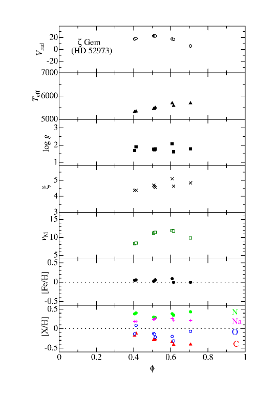
Figure 10: Results of the radial velocity, atmospheric parameters, and elemental abundances derived from each of the 8 spectra of $\zeta$ Gem, plotted against the pulsation phase. Otherwise, the same as in Fig. 7.

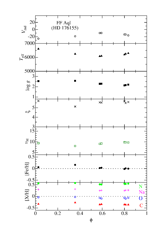
Figure 11: Results of the radial velocity, atmospheric parameters, and elemental abundances derived from each of the 7 spectra of FF Aql, plotted against the pulsation phase. Otherwise, the same as in Fig. 7.

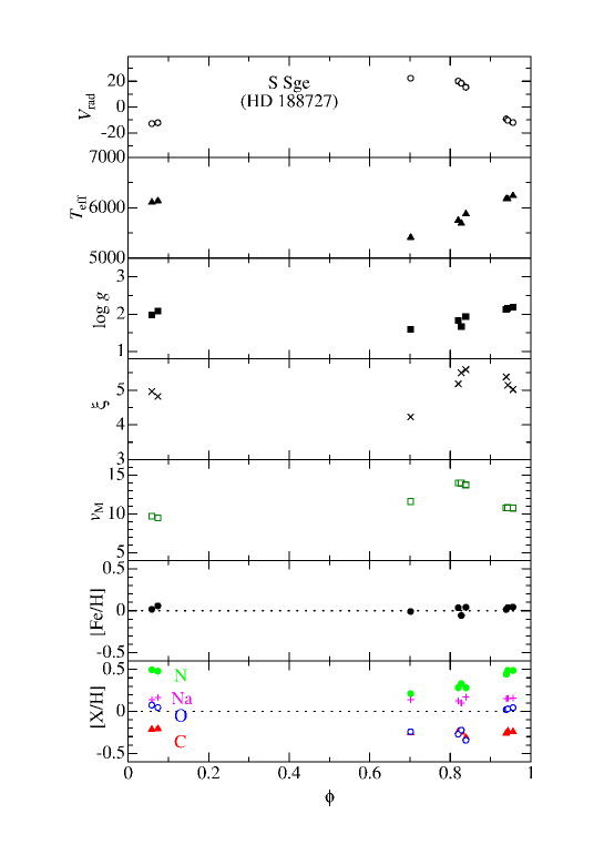
Figure 13: Results of the radial velocity, atmospheric parameters, and elemental abundances derived from each of the 9 spectra of S Sge, plotted against the pulsation phase. Otherwise, the same as in Fig. 7.

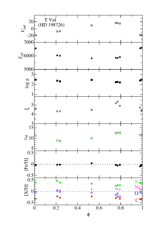
Figure 15: Results of the radial velocity, atmospheric parameters, and elemental abundances derived from each of the 9 spectra of T Vul, plotted against the pulsation phase. Otherwise, the same as in Fig. 7.

Figure 16: Results of the radial velocity, atmospheric parameters, and elemental abundances derived from each of the 9 spectra of DT Cyg, plotted against the pulsation phase. Otherwise, the same as in Fig. 7.

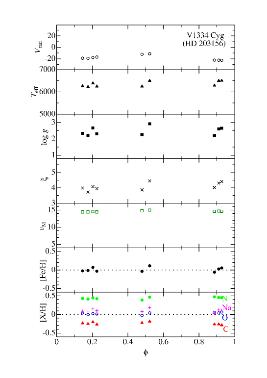
Figure 17: Results of the radial velocity, atmospheric parameters, and elemental abundances derived from each of the 9 spectra of V1334 Cyg, plotted against the pulsation phase. Otherwise, the same as in Fig. 7.

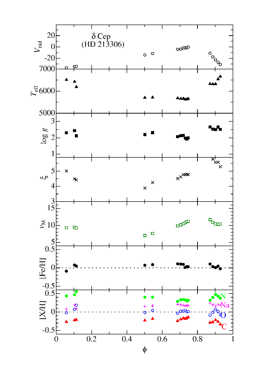
Figure 18: Results of the radial velocity, atmospheric parameters, and elemental abundances derived from each of the 16 spectra of $\delta$ Cep, plotted against the pulsation phase. Otherwise, the same as in Fig. 7.

Figure 19: Phase($\phi$)-dependence of the atmospheric parameters of $\delta$ Cep (HD 213306), where our results and the previous results of other similar “spectroscopic” determinations are overplotted with different symbols: Filled circles — this study, open circles — Kovtyukh & Andrievsky (1999) (spectroscopic $T_{\rm eff}$ and non-standard results for $\log g$, $\xi$,and [Fe/H]), open triangles — Fry & Carney (1997), double circle — Kovtyukh et al. (1994) (note that their $T_{\rm eff}$ was determined from H$\alpha$ and colors), Greek crosses — Luck & Lambert (1985) (spectroscopic $\log g$), diamonds — Andrievsky et al. (2005). (a) $T_{\rm eff}$ vs. $\phi$, (b) $\log g$ vs. $\phi$, (c) $\xi$ vs. $\phi$, and (d) [Fe/H] vs. $\phi$.

Figure 21: $\langle$[X/H]$\rangle$ (mean logarithmic abundance of element X relative to the Sun averaged over different pulsation phases) for each star, plotted against the pulsation period, based on the data (expressed in italic) given in the first line of each section in Table 2: (a) $\langle$[C/H]$\rangle$, (b) $\langle$[N/H]$\rangle$, (c) $\langle$[O/H]$\rangle$, (d) $\langle$[Na/H]$\rangle$, and (e) $\langle$[Fe/H]$\rangle$. The same meanings of the symbols as in Fig. 20, while the attached error bar indicate the extent of the standard deviation ($\sigma$).

Figure 22: Panels (a)–(d) display the correlations between the C, N, O, and Na abundances (averaged over different phases): (a) $\langle$[N/H]$\rangle$ vs. $\langle$[C/H]$\rangle$, (b) $\langle$[Na/H]$\rangle$ vs. $\langle$[O/H]$\rangle$, (c) $\langle\log\epsilon$(N)$\rangle$ vs. $\langle\log\epsilon$(C+O)$\rangle$, and (d) $\langle\log\epsilon$(N)$\rangle$ vs. $\langle\log\epsilon$(C)$\rangle$ [$\langle\log\epsilon$(X)$\rangle\equiv\langle$[X/H]$\rangle$ + $\log\epsilon_{\odot}$]. In panels (c) and (d), the expected relation when $\epsilon$(C)+$\epsilon$(N)+$\epsilon$(O) is conserved at the solar value is also shown. The solid and dashed line in panel (d) correspond to the cases of [O/H] = 0.0 and [O/H] = $-0.1$, respectively. Further, the N-to-C abundance ratio ([N/C] $\equiv$ [N/H]$-$[C/H]) and the sum of C+N+O abundances ($\langle\log\epsilon$(C+N+O)$\rangle$) for each star are plotted against $\log P$ in panels (e) and (f), respectively. Otherwise, the same as in Fig. 20.

References

- [] Andrievsky, S. M., Egorova, I. A., Korotin, S. A., Burnage, R., 2002, A&A, 389, 519
- [] Andrievsky, S. M., Luck, R. E., Kovtyukh, V. V., 2005, AJ, 130, 1880
- [] Benedict, G. F., et al., 2007, AJ, 133, 1810
- [] Bersier, D., Burki, G., Kurucz, R. L., 1997, A&A, 320, 228
- [] Flower, P. J., 1996, ApJ, 469, 355
- [] Fry, A. M., Carney, B. W., 1997, AJ, 113, 1073
- [] Kang, D.-I., Park, H.-S., Han, I.-W., Valyavin, G., Lee, B.-C., Kim, K.-M., 2006, Pub. Korea Astron. Soc., 21, 101
- [] Caputo, F., Bono, G., Fiorentino, G., Marconi, M., Musella, I., 2005, ApJ, 629, 1021
- [] Kiss, L.L., 1998, MNRAS, 297, 825
- [] Kovtyukh, V. V., Andrievsky, S. M., 1999, A&A, 351, 597
- [] Kovtyukh, V. V., Andrievsky, S. M., Belik, S. I., Luck, R. E., 2005a, AJ, 129, 433
- [] Kovtyukh, V. V., Komarov, N. S., Depenchuk, E. A., 1994, Astron. Lett., 20, 177
- [] Kovtyukh, V. V., Wallerstein, G., Andrievsky, S. M., 2005b, PASP, 117, 1173
- [] Kurucz, R. L., 1993, Kurucz CD-ROM, No. 13, ATLAS9 Stellar Atmosphere Program and 2 km/s Grid (Cambridge, MA: Harvard-Smithsonian Center for Astrophysics)555Available at http://kurucz.harvard.edu/PROGRAMS.html.
- [] Kurucz, R. L., Bell, B., 1995, Kurucz CD-ROM, No. 23, Atomic Line Data (Cambridge, MA: Harvard-Smithsonian Center for Astrophysics)666Available at http://kurucz.harvard.edu/LINELISTS.html.
- [] Lambert, D. L., 1992, in Instabilities in evolved super- and hypergiants, ed. C. de Jager, H. Nieuwenhuijzen (Amsterdam: North-Holland), p.156
- [] Lejeune, T., Schaerer, D., 2001, A&A, 366, 538
- [] Leushin, V. V., Topil’skaya, G. P., 1986, Astrophysics, 25, 415
- [] Luck, R. E., Andrievsky, S. M., 2004, AJ, 128, 343
- [] Luck, R. E., Andrievsky, S. M., Fokin, A., Kovtyukh, V. V., 2008, AJ, 136, 98
- [] Luck, R. E., Lambert, D. L., 1981, ApJ, 245, 1018
- [] Luck, R. E., Lambert, D. L., 1985, ApJ, 298, 782
- [] Nissen, P. E., 1993, in Inside the Stars, Proc. IAU Colloq. 137, ASP Conf. Ser. Vol. 40, eds. W. W. Weiss & A. Baglin (Astron. Soc. Pacific: San Francisco), p. 108
- [] Sasselov, D. D., 1986, PASP, 98, 561
- [] Smiljanic, R., Barbuy, B., De Medeiros, J. R., Maeder, A., 2006, A&A, 449, 655
- [] Takeda, Y., 1995, PASJ, 47, 287
- [] Takeda Y., Kambe, E., Sadakane, K., Masuda, S., 2010, PASJ, 62, 1239
- [] Takeda, Y., Ohkubo, M., Sadakane, K., 2002, PASJ, 54, 451
- [] Takeda, Y., Ohkubo, M., Sato, B., Kambe, E., Sadakane, K., 2005, PASJ, 57, 27
- [] Takeda Y., Takada-Hidai M., 1994, PASJ, 46, 395
- [] Takeda Y., Takada-Hidai M., 1995, PASJ, 47, 169
- [] Takeda Y., Takada-Hidai M., 1998, PASJ, 50, 629
- [] Takeda Y., Takada-Hidai M., 2000, PASJ, 52, 113
- [] Takeda, Y., Honda, S., 2005, PASJ, 57, 65
- [] Takeda, Y., Honda, S., Ohnishi, T., Ohkubo, M., Hirata, R., Sadakane, K., 2013, PASJ, No. 3, in press (arXiv: 1212.6318)
- [] Takeda, Y., Sato, B., Murata, D., 2008, PASJ, 60, 781
- [] Takeda Y., Zhao G., Takada-Hidai M., Chen Y.-Q., Saito Y.-J., Zhang H.-W., 2003, ChJAA, 3, 316