The couplings of the Higgs boson and its CP properties from fits
of the signal strengths and their ratios at the 7+8 TeV LHC

Abstract

Using the full set of the LHC Higgs data from the runs at 7 and 8 TeV center of mass energies that have been released by the ATLAS and CMS collaborations, we determine the couplings of the Higgs particle to fermions and gauge bosons as well as its parity or CP composition. We consider ratios of production cross sections times decay branching fractions in which the theoretical (and some experimental) uncertainties as well as as some ambiguities from new physics cancel out. A fit of both the signal strengths in the various search channels that have been conducted, $H\to ZZ,WW,\gamma\gamma,\tau\tau$ and $b\bar{b}$, and their ratios shows that the observed $\sim 126$ GeV particle has couplings to fermions and gauge bosons that are Standard Model–like already at the 68% confidence level (CL). From the signal strengths in which the theoretical uncertainty is taken to be a bias, the particle is shown to be at most 68% CP–odd at the 99%CL and the possibility that it is a pure pseudoscalar state is excluded at the $4\sigma$ level when including both the experimental and theoretical uncertainties. The signal strengths also measure the invisible Higgs decay width which, with the same type of uncertainty analysis, is shown to be $\Gamma_{H}^{\rm inv}/\Gamma_{H}^{\rm SM}\leq 0.52$ at the 68%CL.

1. Introduction

The ATLAS and CMS collaborations have released their analyses of the mass and the production times decay rates of the 126 GeV Higgs–like particle using the full set of data collected so far, $\approx 5$ fb^-1 at $\sqrt{s}=7$ TeV and $\approx 20$ fb^-1 at $\sqrt{s}=8$ TeV CONF-2013-014 ; CONF-2013-034 ; PAS-HIG-12-045 ; PAS-HIG-13-001 . This closes a very successful first run at the LHC, which culminated with the historical discovery of the state in July 2012 ATLAS-disc ; CMS-disc . To be convinced that the observed particle is indeed the Higgs boson that is responsible of the spontaneous breaking of the electroweak symmetry Higgs ; Review , one needs to prove that the particle: $i)$ has spin–zero, $ii)$ is a CP–even state, $iii)$ couples to fermions and gauge bosons proportionally to their masses and, ultimately, $iv)$ has a self–coupling that is also proportional to its mass. While there is little doubt on the spin–zero nature of the observed state ¹, and the probing of the self–coupling has to await for a high–luminosity LHC triple or a future lepton collider, a first determination of the couplings Fits ; EFIT ; Fit-last and the CP–properties CPH-d ; CPH-p can be performed with the current results. The ATLAS and CMS collaborations themselves have given a first “portrait” of the observed particle which indicates that indeed it has the properties of a Higgs boson and even more, the properties of the unique Higgs boson that is predicted in the Standard Model (SM) CONF-2013-014 ; CONF-2013-034 ; PAS-HIG-12-045 ; PAS-HIG-13-001 ; CMS1212 .

However, in the case of the particle coupling determination, the ATLAS and CMS analyses suffer from two serious drawbacks ratios ; Dieter . The first one is that the signal strength modifiers $\mu_{XX}$, that are identified with the Higgs cross section times decay branching ratio normalized to the SM expectation in a given $H\!\to\!XX$ search channel, are affected by large theoretical uncertainties that are now becoming a dominant source of error. Indeed, the combined theoretical uncertainty in the rate of the by far dominant Higgs production process at the LHC, gluon fusion $gg\to H$, is estimated to be of order $\pm 15$–20% LHCXS ; BD even before it is broken into jet categories which significantly increases the uncertainty Scale-H0j ; Scale-H2j . The uncertainty is similar in the vector boson fusion channel when the large contamination from the $gg\to Hjj$ process is taken into account Scale-H2j . Another drawback of the analyses ratios ; Dieter is that they involve strong theoretical assumptions on the total Higgs width since some contributing decay channels not accessible at the LHC are assumed to be SM–like and possible invisible Higgs decays in scenarios beyond the SM are supposed not to occur.

In this letter, we consider ratios of Higgs production cross sections times decay branching fractions in which these two sources of uncertainties and, eventually, also some systematical and parametrical uncertainties such as the error on the luminosity measurement and the one on the Higgs branching ratios ² BD ; BRpaper , should be absent ratios ; Dieter . Using the Higgs signal strengths in which the theoretical uncertainty is taken to be a bias and not a nuisance (as is done generally), as well as the ratios $\mu_{\gamma\gamma}/\mu_{ZZ}$ and $\mu_{\tau\tau}/\mu_{WW}$ which are free from the ambiguities above, we perform a fit of the latest ATLAS and CMS data and conclude that, already at the 68% confidence level (CL), there is no deviation of the Higgs couplings to fermions and gauge bosons from the SM expectation.

On an other front, the attempts made so far for the determination of the CP nature of the particle mainly exploit the kinematical features of the $H\to VV$ decays with $V=W,Z$ CPH-d or the production in the vector boson fusion $V^{*}V^{*}\to H$ and Higgs–strahlung $V^{*}\to VH$ processes CPH-p . Since a CP–odd particle has not have tree level couplings to $VV$ states ³, all these processes project out only the CP–even component of the $HVV$ coupling CP-tt and the considered distributions can be thus only those of a $0^{++}$ state.

We will show that a much better way to measure the CP composition of the observed Higgs state is to consider the measured signal strength in the $H\to VV$ decays; see also Ref. Schwaller . Using $\mu_{ZZ}$, we demonstrate that, if the magnitude of the Higgs couplings to fermions is as in the SM, the pure CP–odd possibility is excluded at the $4\sigma$ level, irrespective of the (mixed CP) Higgs couplings to light fermions.

Finally, assuming that the Higgs couplings to fermions and gauge bosons are SM–like and using mainly the signal strength $\mu_{ZZ}$, one obtains a limit on the rate for invisible Higgs decays, $\Gamma_{H}^{\rm inv}/\Gamma_{H}^{\rm SM}\leq 0.52$ at the 68%CL (see also Ref. Fit-last ; Belanger for an indirect limit), that is stronger than the one obtained from direct invisible Higgs searches portal ; InvATLAS .

2. The signal strengths and their ratios

Let us first summarize the LHC Higgs data collected in the 2011 and 2012 runs for the various SM Higgs decay channels that have been searched for by the ATLAS and CMS collaborations: $H\to ZZ^{*}\to 4\ell^{\pm},\ H\to WW^{*}\to 2\ell 2\nu,\ H\to\gamma\gamma,\ H\to\tau^{+}\tau^{-}$ and $H\to b\bar{b}$; we will ignore the additional search channels $H\to\mu^{+}\mu^{-}$ and $H\to Z\gamma$ (see e.g. Ref. Vega ) for which the sensitivity is still too low. In most cases, the various Higgs production channels have been used: the by far dominant gluon–gluon fusion mechanism $gg\to H$ (ggF) that has the large production rates but also the subleading channels, vector boson fusion (VBF) $qq\to Hqq$ and Higgs–strahlung (HV) $q\bar{q}\to HV$ with $V=W,Z$; the top quark associated $p\bar{p}\to t\bar{t}H$ mechanism (ttH) has too low a cross section to be relevant. At least the ggF and VBF channels have been considered in the $H\to ZZ,WW,\gamma\gamma$ and $H\to\tau^{+}\tau^{-}$ channels, while in the case $H\to\tau^{+}\tau^{-}$ and $H\to WW^{*}\to 2\ell 2\nu$ decays, also the HV production mode in which the $H\to b\bar{b}$ decay has been searched for, has been considered.

ATLAS and CMS have provided the signal strengths for the various final states with a luminosity of, respectively, $\approx 5$ fb^-1 for the 2011 run at $\sqrt{s}=7$ TeV and $\approx 20$ fb^-1 the 2012 run at $\sqrt{s}=8$ TeV. We will identify these $\mu$ values with the Higgs cross section times decay branching fractions normalized to the SM expectation and, for the $H\to XX$ decay, one would have indeed in the narrow width approximation,

$$\mu_{XX}|_{\rm th}\simeq\frac{\sigma(pp\to H\to XX)}{\sigma(pp\to H\to XX)|_{\rm SM}}\simeq\frac{\sigma(pp\to H)\times{\rm BR}(H\to XX)}{\sigma(pp\to H)|_{\rm SM}\times{\rm BR}(H\to XX)|_{\rm SM}}.$$ (1)

From the experimental point of view (and in our fits), this would correspond to

$$\mu_{XX}|_{\rm exp}\simeq\frac{N^{\rm evts}_{XX}}{\epsilon\times\sigma(pp\to H)|_{\rm SM}\times{\rm BR}(H\to XX)|_{\rm SM}\times{\cal L}},$$ (2)

where $N^{\rm evts}_{XX}$ stands for the measured number of events in the $H\to XX$ search channel, $\epsilon$ denotes the selection efficiency and ${\cal L}$ is the luminosity.

In this paper, we consider the decay ratios $D_{XX}$ discussed in Ref. ratios and defined as

$$D_{XX}^{\rm p}=\frac{\sigma^{\rm p}(pp\to H\to XX)}{\sigma^{\rm p}(pp\to H\to VV)}=\frac{\sigma^{\rm p}(pp\to H)\times{\rm BR}(H\to XX)}{\sigma^{\rm p}(pp\to H)\times{\rm BR}(H\to VV)}=\frac{\Gamma(H\to XX)}{\Gamma(H\to VV)}$$ (3)

for a specific production process ${\rm p=ggF,VBF,VH}$ or all (for inclusive production) and for a given decay channel $H\to XX$ when the reference channel $H\to VV$ with $V=W$ or/and $Z$ is used. In these ratios, the cross sections $\sigma(pp\to H)$ and hence, their significant theoretical uncertainties will cancel out as discussed previously, leaving out only the ratio of decay branching fractions and hence of partial decay widths. Thus, the total decay width which includes contributions from channels not under control such as possible invisible Higgs decays, do not appear in the decay ratios $D_{XX}^{\rm p}$. Some common experimental systematical uncertainties such as the one from the luminosity measurement as well as the uncertainties in the Higgs decay branching ratios also cancel out. We are thus, in principle, left with mostly the statistical uncertainty and some systematical errors ⁴.

The ratios $D_{XX}$ involve, up to kinematical factors, only the ratios $|c_{X}|^{2}/|c_{V}|^{2}$ of the reduced couplings of the Higgs boson to the particles $X$ and $V$ compared to the SM expectation, $c_{X}\equiv g_{HXX}/g_{HXX}^{\rm SM}$. $d_{XX}$. For the SM Higgs boson with a mass of $M_{H}=125$ GeV, the kinematical factors can be straightforwardly obtained using the program HDECAY HDECAY for the evaluation of the Higgs branching ratios when the SM inputs recommended by the LHC Higgs working group LHCXS are adopted; they are given in Ref. ratios for the various normalisations (and, for simplicity, are then set to unity in that paper).

In practice, to take into account the fact that there are four different Higgs production channels with different topologies, the cross section part is more involved and the ratio $D_{XX}$ can be more precisely written as

$$D_{XX}\propto\frac{\epsilon^{gg}_{X}\sigma(gg\!\to\!H)\!+\!\epsilon^{\rm VBF}_{X}\sigma(Hqq)\!+\!\epsilon^{HV}_{X}\sigma(HV)+\epsilon^{t\bar{t}H}_{X}\sigma(t\bar{t}H)}{\epsilon^{gg}_{V}\sigma(gg\!\to\!H)+\epsilon^{\rm VBF}_{V}\sigma(Hqq)+\epsilon^{HV}_{V}\sigma(HV)+\epsilon^{t\bar{t}H}_{V}\sigma(t\bar{t}H)}\times\ \frac{\frac{\Gamma(H\to XX)}{\Gamma(H\to XX)|_{\rm SM}}}{\frac{\Gamma(H\to VV)}{\Gamma(H\to VV)|_{\rm SM}}}$$ (4)

where the $\epsilon_{X}^{p}$, provided by the ATLAS and CMS collaborations, denote the experimental efficiencies to select the Higgs events in the $gg$, VBF, $HV$, $t\bar{t}H$ production and $H\to XX$ decay channels (exclusive cut categories are also considered). $D_{XX}$ is only proportional to the above expression due to the presence of another identical ratio of cross sections but within the SM ⁵. Nevertheless for almost the same selection efficiencies, and even for $\epsilon_{X}^{p}=k\epsilon_{V}^{p}$ with $k$ a constant, the expression eq. (4) simplifies to that in eq. (5).

In fact, the decay ratios $D_{XX}$ can be simply written in terms of the signal strengths

$$D_{XX}\hat{=}\frac{\mu_{XX}}{\mu_{VV}}\simeq\frac{\frac{\sigma(pp\to H)\times{\rm BR}(H\to XX)}{\sigma(pp\to H)|_{\rm SM}\times{\rm BR}(H\to XX)|_{\rm SM}}}{\frac{\sigma(pp\to H)\times{\rm BR}(H\to VV)}{\sigma(pp\to H)|_{\rm SM}\times{\rm BR}(H\to VV)|_{\rm SM}}}=\frac{\frac{{\rm BR}(H\to XX)}{{\rm BR}(H\to XX)|_{\rm SM}}}{\frac{{\rm BR}(H\to VV)}{{\rm BR}(H\to VV)|_{\rm SM}}}=\frac{\frac{\Gamma(H\to XX)}{\Gamma(H\to XX)|_{\rm SM}}}{\frac{\Gamma(H\to VV)}{\Gamma(H\to VV)|_{\rm SM}}}=\frac{|c_{X}|^{2}}{|c_{V}|^{2}}$$ (5)

where have used as normalisations in the ratios the channels ⁶ $H\to VV$ with $V\!=\!Z$ or $W$.

Nevertheless, performing the ratios of signal strengths leads to a loss of information and, in some case, we will need at least one signal strength to set the normalisation. Rather than using the global $\mu_{\rm tot}$ value obtained by combining all search channels, we will consider the cleaner $H\to ZZ$ channel alone as it is fully inclusive and thus does not involve the additional large scale uncertainties that occur when breaking the $gg\!\to\!H$ cross section into jet categories ⁷. The combination of the ATLAS and CMS data in the $ZZ$ channel gives

$$\mu_{\rm ZZ}=1.10\pm 0.22^{\rm\;exp}\pm 0.2^{\rm\;th}\,$$ (6)

where the first uncertainty is experimental and the second one theoretical and that we assume to be, conservatively, $\Delta^{\rm th}\!=\!\pm 0.2$. It has been advocated in Ref. ratios ; BD that, since the main effect of the theoretical uncertainty (which has no statistical ground) is to modify the normalisation of the SM cross section, it should be considered as a bias (rather than a nuisance as in the case of the experimental error) and, hence, one needs to perform two separate fits: one with $\mu_{ZZ}\!+\!\Delta^{\rm th}$ and another with $\mu_{ZZ}\!-\!\Delta^{\rm th}$.

3. A combined fit of the Higgs couplings

In order to study the Higgs at the LHC we define the (now usual) effective Lagrangian,

$${\cal L}_{h} = \ c_{W}\ g_{HWW}\ H\ W_{\mu}^{+}W^{-\mu}+\ c_{Z}\ g_{HZZ}\ H\ Z_{\mu}^{0}Z^{0\mu}$$

$$- c_{t}\;y_{t}\;H\bar{t}_{L}t_{R}-c_{c}\;y_{c}\;H\bar{c}_{L}c_{R}-c_{b}\;y_{b}\;H\bar{b}_{L}b_{R}-c_{\tau}\;y_{\tau}\;H\bar{\tau}_{L}\tau_{R}\ +\ {\rm h.c.}$$

where $y_{t,c,b,\tau}=m_{t,c,b,\tau}/v$ are the SM Yukawa coupling constants in the mass eigenbasis ($L/R$ indicates the fermion chirality and we consider only the heavy fermions that have substantial couplings to the Higgs boson), $g_{HWW}=2M^{2}_{W}/v$ and $g_{HZZ}=M^{2}_{Z}/v$ are the electroweak gauge boson couplings and $v$ is the Higgs vacuum expectation value. The $c$ parameters are all defined such that the limit $c\to 1$ corresponds to the SM case. For the present task, we assume no or negligible new contributions to the Higgs couplings to photons or gluons, e.g. as induced by new particles.

We will present the results for the fits of the Higgs signal strengths, $\mu_{i}$ ($i$ labels each channel and cut category investigated), in the plane $c_{f}$ versus $c_{V}$. We have chosen universal coupling corrections, $c_{f}=c_{t}=c_{c}=c_{b}=c_{\tau}$ and $c_{V}=c_{W}=c_{Z}$, for an illustrative purpose. All the Higgs production/decay channels are considered here and the data used are the latest ones and are borrowed from Ref. muTevatron for the Tevatron, from Refs. CONF-2013-012 ; CONF-2013-013 ; CONF-2013-030 ; CONF-2012-170 ; CONF-2012-160 and the combined results of Refs. CONF-2013-014 ; CONF-2013-034 for the ATLAS collaboration as well as Refs. PAS-HIG-12-053 ; PAS-HIG-13-001 ; PAS-HIG-13-002 ; PAS-HIG-13-003 ; PAS-HIG-12-020 ; PAS-HIG-12-045 ; PAS-HIG-13-004 and the combined analysis of Ref. PAS-HIG-12-045 for the CMS collaboration and finally the LHC results presented at the Moriond conference this month Ochando ; InvMoriond .

We will closely follow the procedure of Ref. EFIT (to which we refer for the relevant details) for the fit of these data, with one major difference though, the treatment of the theoretical uncertainty. The errors used in the present fit are those given by the collaborations as quoted above and, thus, contain the experimental and theoretical uncertainties added in quadrature, $\delta\mu_{i}=\sqrt{\delta\mu_{i}|_{\rm exp}^{2}+\delta\mu_{i}|_{\rm th}^{2}}$, which completely dilutes the effect of $\delta\mu_{i}|_{\rm th}$. In the present analysis, we treat the theoretical uncertainty as a bias (and not as if it were associated with a statistical distribution) and perform the fit for the two extremal values of the signal strength : $\mu_{i}|_{\rm exp}[1\pm\delta\mu_{i}/\mu_{i}|_{\rm th}]$ with the theoretical uncertainty $\delta\mu_{i}/\mu_{i}|_{\rm th}$ conservatively assumed to be $20\%$ for both the gluon and vector boson fusion mechanisms.

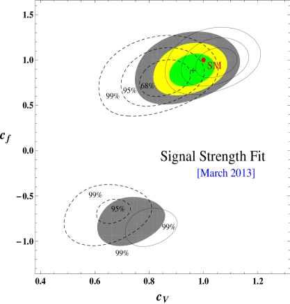
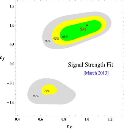
The results of the fit of the data is presented in Fig. 1 and relies on established values PDG of $\Delta\chi^{2}=\chi^{2}-\chi^{2}_{\rm min}$ with the following $\chi^{2}$ function

$$\chi^{2}\ =\ \sum_{i}\frac{[\mu_{i}(c_{f},c_{V})-\mu_{i}|_{\rm exp}]^{2}}{(\delta\mu_{i})^{2}}\ .$$ (8)

In addition to the fit that is usually performed, leading to the colored regions on the left plot of Fig. 1 for the best fits at the $1\sigma,2\sigma$ and $3\sigma$ levels in the $c_{f}$ versus $c_{V}$ plane ⁸, we also present the results of the fit for a treatment of the theoretical uncertainty as a bias. The value, $\mu_{i}|_{\rm exp}+(\delta\mu_{i}/\mu_{i}|_{\rm th})\Big{|}\mu_{i}|_{\rm exp}\Big{|}$, corresponds to the plain contours on Fig. 1 while the dashed contours are for the lower $\mu_{i}|_{\rm exp}$ expectations (negative sign in front of the error). The distances between the two contours represent the theoretical uncertainty induced on the fitted parameters. The treatment of the theoretical uncertainty as a bias is also illustrated on the right plot of Fig. 1 using colored domains.

Figure 1: Left plot Best-fit regions at $68.27\%{\rm CL}$ (green), $95.45\%{\rm CL}$ (yellow) and $99.73\%{\rm CL}$ (grey) in the plane $c_{f}$ versus $c_{V}$, based on the $\chi^{2}$ function of eq. (8); the best-fit location is indicated by a (black) cross. The ‘concentric’ best-fit domains at the same CLs obtained also from $\chi^{2}$ but for the two extreme theoretical predictions – upper (plain contours) and lower (dashed contours) – of the Higgs signal strengths, are presented. The SM (red) point at $c_{f}=c_{V}=1$ is also shown. Right plot Best-fit domains at the $68.27\%{\rm CL}$ (green), $95.45\%{\rm CL}$ (yellow) and $99.73\%{\rm CL}$ (light grey) based on the $\chi^{2}$ function; these domains were obtained by varying continuously the Higgs signal strengths from their lowest to highest theoretical predictions.

A first conclusion that can be drawn from this figure is that, with the latest LHC data, in particular the new CMS di-photon rate which has no excess compared to (and is even slightly below) the SM expectation, the SM point is now included inside the $1\sigma$ domain. Before the CMS update, there was a large deviation in the di–photon channel which triggered discussions about the possibility that $c_{f}<0$ (as shown in the figure for the $2\sigma$ and $3\sigma$ regions) which leads to a constructive interference between the top quark and $W$-boson loop contributions to increase the di-photon rate. This possibility has been elaborated within several effective scenarios in the recent literature to generate such a di–photon enhancement (see examples in Ref. Fits ).

The statement that the fit result is compatible with the SM expectation is true regardless of the method chosen to implement the theoretical uncertainty. Nevertheless, it appears clearly on the figure that treating this uncertainty as a bias enhances significantly its effects in the $c$-parameter determination. For instance, the entire $1\sigma$ domain on the plot is larger when taking into account the possible shifts due to the theoretical uncertainty.

As this theoretical uncertainty cancels out in the ratios $D_{XX}$ of signal strengths of eqs. (4,5), we have performed a fit based on the $\chi_{R}^{2}$ function ⁹:

$$\chi^{2}_{R}\ =\ \frac{[D_{\gamma\gamma}^{gg}(c_{f},c_{V})-\frac{\mu_{\gamma\gamma}}{\mu_{ZZ}}|^{gg}_{\rm exp}]^{2}}{\big{[}\delta(\frac{\mu_{\gamma\gamma}}{\mu_{ZZ}})_{gg}\big{]}^{2}}+\frac{[D_{\tau\tau}^{gg}(c_{f},c_{V})-\frac{\mu_{\tau\tau}}{\mu_{WW}}|^{gg}_{\rm exp}]^{2}}{\big{[}\delta(\frac{\mu_{\tau\tau}}{\mu_{WW}})_{gg}\big{]}^{2}}+\frac{[D_{\tau\tau}^{\rm VBF}(c_{f},c_{V})-\frac{\mu_{\tau\tau}}{\mu_{WW}}|^{\rm VBF}_{\rm exp}]^{2}}{\big{[}\delta(\frac{\mu_{\tau\tau}}{\mu_{WW}})_{\rm VBF}\big{]}^{2}}.$$ (9)

We have considered the inclusive di-photon channels of CMS PAS-HIG-13-001 ; Ochando and ATLAS CONF-2013-012 that are largely dominated the ggF mechanism. Regarding the $ZZ$ final state in ATLAS CONF-2013-013 and CMS PAS-HIG-13-002 , we have also used inclusive production ¹⁰. Finally, for the $WW$ and $\tau\tau$ searches in ATLAS CONF-2013-030 ; CONF-2012-160 and in CMS PAS-HIG-13-003 ; PAS-HIG-13-004 , we have selected Higgs production in ggF with an associated 0/1 jet or the VBF production mechanism. Hence for both ATLAS and CMS, the situation is equivalent in a good approximation to have vanishing selection efficiencies except, $\epsilon_{gg}^{Z}\simeq\epsilon_{gg}^{\gamma}\simeq 1$ and $\epsilon_{gg}^{\tau}\simeq\epsilon_{gg}^{W}\simeq 1$ or $\epsilon_{\rm VBF}^{\tau}\simeq\epsilon_{\rm VBF}^{W}\simeq 1$, so that the theoretical predictions for the ratios simply read as in eq. (5).

Figure 2: Left: Best-fit regions at $68.27\%{\rm CL}$ (green), $95.45\%{\rm CL}$ (yellow) and $99.73\%{\rm CL}$ (grey) in the plane $c_{f}$ versus $c_{V}$, based on the $\chi_{R}^{2}$ function. The best-fit (dotted) contours obtained from the $\chi^{2}$ function in case of a theoretical error added in quadrature (as in Fig. 1) are superimposed (in red). The associated best-fit point (cross) and SM (red) point are also shown. Right: Same plot as the left one but the best-fit domains from the $\chi^{2}$ analysis are now derived for the two extreme theoretical predictions of the signal strengths (as in Fig. 1).

The combined ratio values measured by the ATLAS and CMS collaborations are

$$\frac{\mu_{\gamma\gamma}}{\mu_{ZZ}}\Big{|}_{\rm exp}=1.1^{+0.4}_{-0.3}~{},\ \ \frac{\mu_{\tau\tau}}{\mu_{WW}}\Big{|}^{\rm VBF}_{\rm exp}=-0.24\pm 0.83\ \ {\rm and}\ \ \frac{\mu_{\tau\tau}}{\mu_{WW}}\Big{|}^{gg}_{\rm exp}=1.2\pm 0.75$$ (10)

The errors $\delta(\mu_{\gamma\gamma}/{\mu_{ZZ}})$ and $\delta({\mu_{\tau\tau}}/{\mu_{WW}})$ are computed assuming no correlations between the different final state searches. These uncertainties on the ratios are derived from the individual errors, $\delta\mu_{i}$ – provided in the experimental papers – and are thus also dominated by the experimental uncertainties, e.g. $\delta({\mu_{\gamma\gamma}}/{\mu_{ZZ}})\approx\delta({\mu_{\gamma\gamma}}/{\mu_{ZZ}})|_{\rm exp}$, as expected from the fact that the theoretical uncertainty largely cancels in ratios $D_{\gamma\gamma}$ and $D_{\tau\tau}$. These ratios are given by

$$D_{\gamma\gamma} \simeq \frac{1}{|c_{Z}|^{2}}\ \bigg{\{}\frac{\big{|}\frac{1}{4}c_{W}A_{1}[m_{W}]+(\frac{2}{3})^{2}c_{t}A[m_{t}]+(-\frac{1}{3})^{2}c_{b}A[m_{b}]+(\frac{2}{3})^{2}c_{c}A[m_{c}]+\frac{1}{3}c_{\tau}A[m_{\tau}]\big{|}^{2}}{\big{|}\frac{1}{4}A_{1}[m_{W}]+(\frac{2}{3})^{2}A[m_{t}]+(-\frac{1}{3})^{2}A[m_{b}]+(\frac{2}{3})^{2}A[m_{c}]+\frac{1}{3}A[m_{\tau}]\big{|}^{2}}\bigg{\}}$$

$$D_{\tau\tau} \simeq \frac{|c_{\tau}|^{2}}{|c_{W}|^{2}}\ ,$$ (11)

where $A[m]\equiv A_{1/2}[\tau(m)]$ and $A_{1}[\tau(m)]$ are respectively the form factors for spin 1/2 and spin 1 particles Review normalized such that $A[\tau(m)\ll 1]\to 1$ and $A_{1}[\tau(m)\ll 1]\to-7$ with $\tau(m)=M_{H}^{2}/4m^{2}$ and, for $m_{H}\simeq 125$ GeV, one has $A_{1}[\tau(m_{W})]\simeq-8.3$ and $A_{1/2}[\tau(m_{t})]\approx 1$.

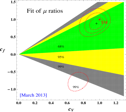
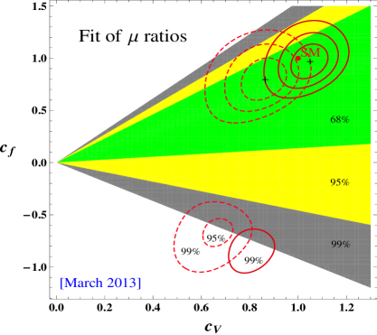
In Figure 2, we show the results from fitting the Higgs decay ratios through the function $\chi_{R}^{2}$. In the left panel, the best-fit domains obtained e.g. at $1\sigma$ do not exclude parts of the $1\sigma$ regions obtained from $\chi^{2}$; such a compatibility was expected since the main theoretical uncertainty cancels out in the $D_{XX}$ ratios and is negligible for the signal strengths since it is added in quadrature to the experimental error as already described. The domains from $\chi^{2}$ are even more restricted as ${\it(i)}$ this function exploits the full experimental information on the Higgs rates and not only on the ratios and ${\it(ii)}$ the experimental error on a ratio of rates is obviously higher than on the rates alone.

In the case where the theoretical error for each Higgs channel is taken into account as a bias, the best-fit contours span wider regions of the parameter space. This could be seen in Fig. 1 and the same contours appear in the left–hand side of Fig. 2 as well as in its right–hand side part where the theoretical uncertainty enters as a bias for $\chi^{2}$. In the latter case, the large $1\sigma$ domain from $\chi_{R}^{2}$ excludes a small part of the $1\sigma$ region (near the SM point) obtained from $\chi^{2}$. Besides, the lower $95.45\%{\rm CL}$ region from the $\chi^{2}$ fit is completely excluded by the $\chi_{R}^{2}$ domain (in yellow) at the same ${\rm CL}$. In conclusion, within the more realistic case of treating the theoretical uncertainty as a bias, the $\chi_{R}^{2}$ domains can thus play an important role by excluding parts of the $\chi^{2}$-fit regions; this is due to the increased contribution of the theoretical error, in $\chi^{2}$, which does not affect $\chi_{R}^{2}$.

Figure 3: Best-fit regions at $68.27\%{\rm CL}$ (green), $95.45\%{\rm CL}$ (yellow) and $99.73\%{\rm CL}$ (grey) in the plane $c_{t}$ versus $c_{V}$ as obtained from a three-dimensional fit (whose best-fit point is the black cross on the central plot) of the 3 free parameters, $c_{f}$, $c_{t}$, $c_{V}$, based on the $\chi^{2}_{R}$ function. The three two-dimensional plots correspond to the slices of these three-dimensional domains at $c_{f}=0.52$, $1.14$ and $1.55$. Superimposed are the best-fit domains at $68.27\%{\rm CL}$, $95.45\%{\rm CL}$, $99.73\%{\rm CL}$ obtained from $\chi^{2}$ for the two theoretical signal strength predictions – upper (red plain) and lower (red dashed contours).

In Fig. 3, we present the three-dimensional $\chi^{2}$-fit results in the case where the parameters $c_{f}$, $c_{t}$ and $c_{V}$ are free. It shows how precisely are presently known the top quark Yukawa and the gauge boson interactions with the Higgs scalar (in the case of a preserved custodial symmetry). For either lower (left plot) or higher (right plot) bottom quark Yukawa couplings as compared to the SM, the size of the characteristic $1\sigma$ regions decrease significantly, which also gives an idea of the present knowledge of the coupling $c_{b}$. This more realistic three-dimensional fit illustrates as well the potential interest of the $\chi^{2}_{R}$-fit : for instance, one observes on the central plot, that it excludes at $1\sigma$ the lower-right (i.e. the dysfermiophilia solution $c_{t}<0$) and upper-left (i.e. its almost symmetric domain) $1\sigma$ regions resulting from the $\chi^{2}$-fit.

Since $\chi_{R}^{2}$ is only affected by the experimental uncertainty, it is interesting to quantify the evolution of the fit when the experimental systematic and statistical errors are reduced EurStrat . For this purpose, we combine the present measurements with the expected results from the $14$ TeV LHC in each channel investigated by ATLAS and CMS. We assume the central values at $14$ TeV to be identical to those from the combination of the $7$ and $8$ TeV data, and that the future experimental errors, $\delta\mu_{i}|_{\rm exp}$, will reduce essentially like the inverse of the square roots of number of events, $\sqrt{\sigma_{i}{\cal L}}$ with ${\cal L}$ the integrated luminosity ¹¹.

The estimated $\chi^{2}$ fit results at $14$ TeV are presented in Fig. 4 assuming luminosities of ${\cal L}\equiv 300$ and $3000$ fb^-1 EurStrat . The behavior of the best-fit $\chi_{R}^{2}$ regions appearing in the figure originates from the compensation between the enhancement of $\Gamma(H\!\to\!\gamma\gamma)$ and that of $\Gamma(H\!\to\!ZZ)$ as $c_{V}$ increases, leading to relatively stable $D_{\gamma\gamma}$ values; the increase of $\Gamma(H\!\to\!\tau\tau)$ and $\Gamma(H\!\to\!WW)$ with increasing $c_{\tau}$ or $c_{W}$ also compensate each other in $D_{\tau\tau}$. Best-fit values of $c_{f}$ and $c_{V}$ in Fig. 4 would be illustrative only since the precise central values are of course not yet known, neither the exact experimental uncertainties. However, the above estimation of the statistical error provides an indication of the typical relative sizes of the best-fit $\chi^{2}$ and $\chi_{R}^{2}$ domains in the future.

Figure 4: Best-fit regions at $68.27\%{\rm CL}$ (green), $95.45\%{\rm CL}$ (yellow) and $99.73\%{\rm CL}$ (grey) in the plane $c_{f}$ versus $c_{V}$, based on the $\chi_{R}^{2}$ function and including hypothetical data from the $14$ TeV LHC with ${\cal L}=300$ fb^-1 [left plot] or $3000$ fb^-1 [right plot]. The best-fit $\Delta\chi^{2}$ contours at $95.45\%{\rm CL}$ and $99.73\%{\rm CL}$ obtained in the same conditions, for the two extreme theoretical predictions of signal strengths (red plain and dashed ellipses), are superimposed; the $68.27\%{\rm CL}$ domain presented (in red) was obtained by varying continuously the signal strengths from their lowest to highest theoretical predictions. So typically the length of this domain indicates the theoretical uncertainty and its width the experimental error. The exactly symmetric domains, obtained via $c_{f}\to-c_{f}$, $c_{V}\to-c_{V}$, are not shown.

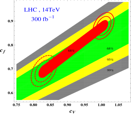
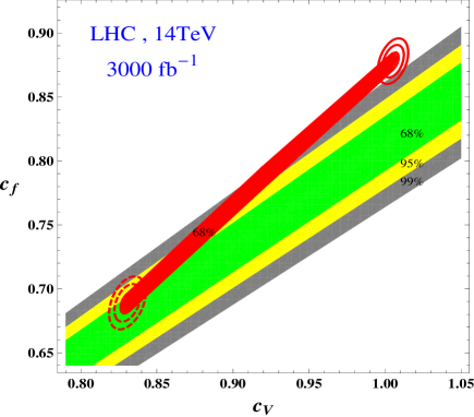
The main features that the plots of Fig. 4 exhibit are that when increasing the luminosity and hence, reducing the experimental error as shown by the smaller ellipses on the right plot, the $\chi^{2}$-fit reaches the level where the theoretical error is dominating and fixes the typical uncertainty scale (stable red band length on the two plots), whereas for the $\chi_{R}^{2}$-fit in which the theoretical uncertainty is absent, the precision obtained on the couplings $c_{f}$ and $c_{V}$ improves as long as the experimental error decreases (decrease of the colored region widths on the right plot). Thus, for high LHC luminosities, the fit of the decay ratios will play a crucial role and will have to be combined with the common Higgs rate fit, as illustrated on the right plot of Fig. 4: there for instance the $1\sigma$ region from $\chi^{2}$ (typically the red band) is wider than when restricted to its intersection with the $\chi_{R}^{2}$ domain at $1\sigma$ (green band). This corresponds, to an improvement of the whole accuracy from $\sim 10\%$ down to $\sim 5\%$ on both $c_{f}$ and $c_{V}$; with such accuracies one starts to be really sensitive to deviations in the Higgs couplings arising in supersymmetric theories or composite Higgs models as, for instance, discussed in Ref. Gupta .

Figure 5: Best-fit regions at $68.27\%{\rm CL}$ (green), $95.45\%{\rm CL}$ (yellow) and $99.73\%{\rm CL}$ (grey) in the plane $c_{f}$ versus $c_{V}$, based on the $\chi_{R}^{2}$ function and including hypothetical data from the $14$ TeV LHC with ${\cal L}=3000$ fb^-1 [as in Fig. 4]. The best-fit $\Delta\chi^{2}$ contours at $68.27\%{\rm CL}$, $95.45\%{\rm CL}$, $99.73\%{\rm CL}$ obtained in the same conditions, and with the theoretical error added in quadrature, are superimposed as dotted (red) contours; the best central point is indicated as a (black) cross.

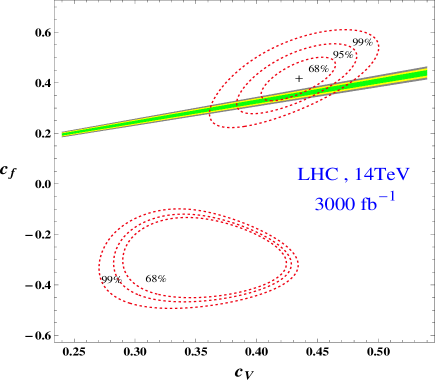
For illustration, we present in Fig. 5 the expected results of the $\chi^{2}$ fit, at $14$ TeV with ${\cal L}\equiv 3000$ fb^-1, when adding the theoretical error to the experimental one in quadrature; the associated best-fit regions are obviously different from the pairs of ellipse-like best-fit domains obtained for a theoretical uncertainty treated as a bias [Fig. 4]. Furthermore, in Fig. 5, there exist best-fit regions at negative $c_{f}$ values. This comparison between Fig. 4 and Fig. 5 clearly allows to convince oneself that the choice of the treatment of theoretical errors will be crucial for the determination of the Higgs couplings. Nevertheless, even in the case of a theoretical uncertainty combined in quadrature, the fit of rate ratios (independent of the theoretical error and presented again in Fig. 5) allows to select a sub-part of the $1\sigma$, $2\sigma$, $3\sigma$ ellipses derived from the signal strength fit.

4. The parity or CP–composition of the Higgs boson

As mentioned in the introduction, the observables such as correlations in Higgs decays into vector boson pairs CPH-d or in Higgs production with or through these states CPH-p that are usually used to probe the Higgs parity project out only the CP–even component of the $HVV$ coupling even if the state has both CP–even and CP–odd components. Thus, in these CP studies, one is simply verifying, a posteriori, that a CP–even Higgs state has been indeed produced. The $HVV$ coupling takes the general form (here, we assume $c_{V}>0$)

$$g_{HVV}^{\mu\nu}=-i\ c_{V}(M_{V}^{2}/v)\;g^{\mu\nu}$$ (12)

where $c_{V}$ measures the departure from the SM: $c_{V}\!=\!1$ for a pure CP–even state with SM–like couplings and $c_{V}=0$ for a pure CP–odd state. Indeed, the coupling of a pseudoscalar $A$ state to $W/Z$ bosons is zero at tree-level and is generated only through loop corrections which are expected to tiny. The measurement of $c_{V}$ should allow to determine the CP composition of a Higgs boson if it is indeed a mixture of CP–even and CP–odd states.

However, having $c_{V}\!\neq\!1$ does not automatically imply that the observed state has a pseudoscalar component. As a matter of fact, the Higgs sector could be enlarged to contain other neutral Higgs particles $H_{i}$ that have not been detected so far because they are too heavy or too weakly coupled. In this case, the sum of the squared couplings of each state $H_{i}$ to gauge bosons, $c_{Vi}^{2}\,g_{HVV}^{2}$, should reduce to the SM Higgs coupling, $g_{HVV}^{2}$. Hence, $c_{V}^{2}\!<\!1$, could mean that there are other CP–even states which share the SM Higgs coupling to $VV$ with the observed Higgs boson. Nevertheless, in all cases, the quantity $\kappa_{\rm CP}=1-c_{V}^{2}$ gives an upper bound on the CP–odd contribution to the $HVV$ coupling ¹².

In contrast to the couplings to massive gauge boson, the CP–even and CP–odd components of the state can couple to fermions with the same magnitude and one can write

$$g_{Hff}=-i\frac{m_{f}}{v}\bigg{[}{\rm Re}\,(c_{f})+i\ {\rm Im}\,(c_{f})\,\gamma_{5}\bigg{]}$$ (13)

where in the SM one has Re$(c_{f})\!=\!1$ and Im$(c_{f})\!=\!0$ but in general, the normalisation of the coupling, ${\rm Re}(c_{f})^{2}+{\rm Im}(c_{f})^{2}=|c_{f}|^{2}$, should be taken arbitrary as in the previous section.

Hence, one can consider the same effective Lagrangian as in eq. (3. A combined fit of the Higgs couplings) where $c_{V}=c_{Z}=c_{W}$ represents exclusively the CP–even component of the observed boson assumed to be one eigenstate of an enlarged Higgs sector. In contrast, the $c_{f}\!=\!c_{b}\!=\!c_{c}\!=\!c_{\tau}$ and $c_{t}$ parameters for light fermions and the top quark contain the CP compositions of eq. (13) with the possibility of a deviation of the normalisation $|c_{f}|^{2}$ compared to the SM Yukawa interaction.

In the case of the light fermions, one has $M_{H}\gg m_{f}$ so that chiral symmetry holds and the partial decay widths (the only place where they enter if one neglects their tiny contribution to the loop induced vertices) can be simply written as $\Gamma(H\to f\bar{f})\propto{\rm Re}(c_{f})^{2}+{\rm Im}(c_{f})^{2}\propto|c_{f}|^{2}$ and the discussion in the previous section should entirely hold.

In the case of the top quark, the situation is different as $m_{t}\!>\!M_{H}$. The top quark enters the $Hgg$ and $H\gamma\gamma$ vertices and the loop form factors for the CP–even $A_{1/2}^{H}$ and CP–odd $A_{1/2}^{A}$ parts are in principle different Review . Fortunately, in these vertices the approximation $m_{t}\gg M_{H}$ is extremely good and in this limit, the form factors take simple forms: $A_{1/2}^{H}=\frac{4}{3}$ and $A_{1/2}^{A}=2$. Ignoring the small contributions of the light fermions for simplicity, the Higgs rates normalized to the SM expectations can be written as,

$$\frac{\Gamma(H\to\gamma\gamma)}{\Gamma(H\to\gamma\gamma)|_{\rm SM}} \simeq \frac{\big{|}\frac{1}{4}c_{W}A_{1}[m_{W}]+(\frac{2}{3})^{2}{\rm Re}(c_{t})\big{|}^{2}+|(\frac{2}{3})^{2}\frac{3}{2}{\rm Im}(c_{t})|^{2}}{\big{|}\frac{1}{4}A_{1}[m_{W}]+(\frac{2}{3})^{2}\big{|}^{2}}$$

$$\frac{\sigma(gg\to H)}{\sigma(gg\to H)|_{\rm SM}} = \frac{\Gamma(H\to gg)}{\Gamma(H\to gg)|_{\rm SM}}\simeq\big{|}{\rm Re}(c_{t})\big{|}^{2}+|\frac{3}{2}{\rm Im}(c_{t})\big{|}^{2}$$ (14)

with $A_{1}[m_{W}]\simeq-8.3$ for $M_{H}\approx 125$ GeV. For a pure pseudoscalar state, Re$(c_{t})=0$, there is no $W$ contribution to the $H\to\gamma\gamma$ rate; there are also no $H\to ZZ$ and $WW$ decays, a possibility that is clearly excluded by the present data as the $4\ell$ and $2\ell 2\nu$ signals have been observed. To quantify the degree of exclusion of this possibility, one needs to measure $\kappa_{\rm CP}=1-c_{V}^{2}$ (and ideally, independently of the fermion couplings $c_{f}$).

Figure 6: Best-fit regions at $68.27\%{\rm CL}$ (green), $95.45\%{\rm CL}$ (yellow) and $99.73\%{\rm CL}$ (grey) in the plane $1-c^{2}_{V}$ versus Im$(c_{t})$ for $|c_{t}|^{2}\!=\!|c_{f}|^{2}\!=\!1$ ; these regions are obtained from a two-dimensional fit based on the $\chi^{2}_{R}$ function. Superimposed are the best-fit regions at $68.27\%{\rm CL}$, $95.45\%{\rm CL}$, $99.73\%{\rm CL}$ obtained from $\chi^{2}$ for the two theoretical signal strength predictions (plain and dashed contours in red). The SM (red) point is represented at the origin together with the best-fit points (the two black crosses) for the $\chi^{2}$ fits.

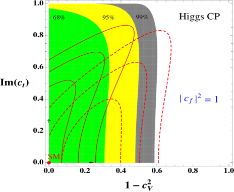
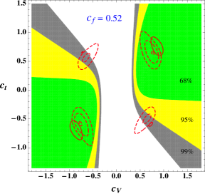
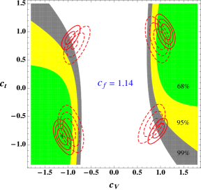
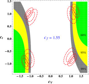
Based on these rates, one can perform a fit using the same $\chi^{2}$ function as in eq. (8) but with the dependence, $\chi^{2}=\chi^{2}[\mbox{\rm Re}(c_{t}),\mbox{\rm Im}(c_{t}),c_{f},c_{V}]$. The numerical results are displayed in Fig. 6 for the $\chi^{2}$-fit and the $\chi^{2}_{R}$-fit which reveals itself to be useful as well for measuring the CP-odd component of the Higgs boson. In this case, we have made the simplifying assumption (besides $c_{V}\geq 0$) that the absolute normalisation of the fermion couplings is the same as in the SM, $|c_{t}|^{2}\!=\!|c_{f}|^{2}\!=\!1$, but in the case of the top quark, $\mbox{\rm Im}(c_{t})$ is assumed to be free. We assume ${\rm Re}(c_{t})\geq 0$ and the obtained plot is symmetric under ${\rm Im}(c_{t})\to-{\rm Im}(c_{t})$.

The conclusion is that, at the 99.73%CL or at the $3\sigma$ level, the CP–odd component of the observed Higgs boson obeys the upper bound $\kappa_{\rm CP}=1-c_{V}^{2}<0.68$. A pure CP–odd Higgs state, i.e. the case $\kappa_{\rm CP}\approx 1$, is excluded with more than $4\sigma$. This is much more severe than the constraint from the correlations in $H\to ZZ$ decays, which (with its inherent limitation discussed above) allows only a $\raisebox{-3.69899pt}{~{}\shortstack{$<$ \\ [-0.07cm] $\sim$}}~{}3\sigma$ discrimination between the CP–even and CP–odd cases CONF-2013-034 ; PAS-HIG-12-045 .

5. The invisible Higgs decay width

Figure 7: Domains at $1\sigma$ (green), $2\sigma$ (yellow) from the central value of $\mu_{ZZ}$, in the plane $c_{V}$ (left plot) or $c_{f}$ (right plot) versus $\Gamma_{H}^{\rm inv}/\Gamma_{H}^{\rm SM}$ [$\Gamma_{H}^{\rm SM}$ being the total SM Higgs width] for $c_{t}\!=\!1$ and $c_{f}\!=\!1$ (left plot) or $c_{V}\!=\!1$ (right plot). The dependence of these constraints on the theoretical uncertainties is illustrated by the (black) curves which indicate the other possible extreme domains. The direct upper limit on $\Gamma_{H}^{\rm inv}$ from invisible searches at LHC (derived for $c_{V}\!=\!1$) InvATLAS ; InvMoriond is shown on the right plot.

In the previous discussion, the signal strength $\mu_{ZZ}$ in the channel $H\to ZZ\to 4\ell^{\pm}$ played a prominent role because the theoretical ambiguities are minimised: the measurement is inclusive and does not involve the additional theoretical uncertainties that are introduced when breaking the cross section into jet categories and there is no loop induced new physics effect as in the $H\to\gamma\gamma$ case; besides that, it is the most accurate single signal strength measurement. One can also use $\mu_{ZZ}$ for the determination of the invisible Higgs decay width which enters in the signal strength through the total decay width $\Gamma_{H}^{\rm tot}$, $\mu_{ZZ}\propto\Gamma(H\to ZZ)/\Gamma_{H}^{\rm tot}$ with

$$\Gamma_{H}^{\rm tot}=\Gamma_{H}^{\rm inv}+\Gamma_{H}^{\rm SM}(c_{f},c_{V})$$ (15)

$\Gamma_{H}^{\rm SM}(c_{f},c_{V})$ is the SM total width which is calculated with free coefficients $c_{f}$ and $c_{V}$ and including the state-of-the art radiative corrections BD ; BRpaper . One can write the $ZZ$ signal strength as a function of $\Gamma_{H}^{\rm inv}$ and the Higgs couplings, $\mu_{ZZ}|_{\rm th}=\mu_{ZZ}(\Gamma_{H}^{\rm inv},c_{V},c_{t},c_{f}=c_{c}=c_{b}=c_{\tau})$, and impose that it lies within its $1\sigma$ or $2\sigma$ ranges. This restricts the parameter space to specific regions as is shown in Fig. 7 where in the left-hand hand side $c_{f}$ is SM–like and $c_{V}$ is varied and in the right–hand side, it is the opposite $c_{f}$ is varied while $c_{V}=1$.

On the figure, we also display for comparison the recent direct limit InvATLAS ; InvMoriond on the invisible Higgs width obtained from combining the 7+8 TeV LHC data in the $q\bar{q}\to ZH\to Z+\not E_{T}$ direct search channel. This gives $B_{H}^{\rm inv}<65\%$ at the $95.45\%{\rm CL}$ if the assumption $c_{V}=1$ is made. With the simplifying $c_{f}=c_{V}=1$ assumption, the indirect limit on the invisible width that one obtains from the signal strengths is better, as can be seen from the figure; at $1\sigma$, it reads as

$$\mu_{\rm inv}=\Gamma_{H}^{\rm inv}/\Gamma_{H}^{\rm SM}\leq 0.52\ @68\%{\rm CL}$$ (16)

This limit is at least a factor of two worse than those obtained in the similar fits of Refs. Fit-last using the latest LHC data, the reason being that, here, we assume a 20% theoretical uncertainty on the Higgs production cross sections that we treat as a bias and do not combine quadratically with the experimental uncertainty.

6. Conclusion

We have analyzed the Higgs production cross sections at the LHC for the different Higgs decay channels that have been searched for, $H\to WW,ZZ,\tau\tau,b\bar{b}$ and $H\to\gamma\gamma$. Using the latest results given by the ATLAS and CMS collaborations with the $\approx 25$ fb^-1 data collected in the runs at $\sqrt{s}=7$ and 8 TeV, we have first performed a fit of the Higgs couplings to fermions and massive gauge bosons and shown that they are now compatible with the SM expectation at the $1\sigma$ level. The accuracy of the various experimental measurements is now almost saturated by the theoretical uncertainties stemming from QCD.

We have argued that ratio of cross sections times branching ratios in different Higgs search channels are essentially free from these uncertainties and do not require further theoretical assumptions, on the total Higgs decay width for instance. These ratios, in particular in the $H\to\gamma\gamma$ v.s. $H\to ZZ$ and $H\to\tau\tau$ v.s. $H\to WW$ channels, are being measured quite accurately already with the present data and provide tests of the SM predictions in a less model–dependent way. We show that at the 14 TeV LHC with a high luminosity, 300 fb^-1 and even 3000 fb^-1, they could allow the measurement of ratios of Higgs couplings with an accuracy at the level of a few percent which should allow to test the small deviations expected in realistic new physics models.

In a second part of this paper, we have considered together with the ratios of cross sections times branching ratios in the most important search channels, the signal strength in the extremely clean $H\to ZZ$ channel in which the theoretical uncertainty is taken to be a bias. We have then shown that first, the particle observed at the LHC is at most 68% CP–odd at the 99%CL and the possibility that it is a pure pseudoscalar state (and hence does not couple to $ZZ$ states at tree–level) is excluded at the $4\sigma$ level when including both the experimental and theoretical uncertainties. The signal strengths in the $H\to ZZ$ channel also measure the invisible Higgs decay width which is shown to be $\Gamma_{H}^{\rm inv}/\Gamma_{H}^{\rm SM}\leq 0.52$ at the 68%CL if the Higgs couplings to fermions and gauge bosons are assumed to be SM–like.

All these results give us great confidence that the state observed at the LHC in July 2012 is indeed a Higgs particle and, more than that, it resembles very closely to the Higgs particle predicted in the Standard Model.

Acknowledgements: We thank Aleksandr Azatov, Henri Bachacou, Oscar J. P. Eboli and Rohini Godbole for discussions. AD thanks the CERN theory division for the kind hospitality and GM the University of Warsaw where this work was finalized. This work is supported by the ERC Advanced Grant Higgs@LHC. GM is also supported by the “Institut Universitaire de France”, the ANR CPV-LFV-LHC project and the Orsay Labex P2IO.

References

- (1) The ATLAS collaboration, ATLAS-CONF-2013-014.
- (2) The ATLAS collaboration, ATLAS-CONF-2013-034.
- (3) The CMS collaboration, CMS PAS-HIG-12-045.
- (4) The CMS collaboration, CMS PAS-HIG-13-001.
- (5) The ATLAS collaboration, arXiv:1207.7214 [hep-ex].
- (6) The CMS collaboration, arXiv:1207.7235 [hep-ex].
- (7) P. Higgs, Phys. Lett. 12 (1964) 132; Phys. Rev. Lett. 13 (1964) 506; F. Englert and R. Brout, Phys. Rev. Lett. 13 (1964) 321; G. Guralnik, C. Hagen and T. Kibble, Phys. Rev. Lett. 13 (1964) 585; S. Weinberg, Phys. Rev. Lett. 19 (1967) 1264.
- (8) For a review of the SM Higgs boson, see: A. Djouadi, Phys. Rept. 457 (2008) 1.
- (9) L. Landau, Dokl. Akad. Nauk Ser. Fiz. 60 (1948) 207; C. Yang, Phys. Rev. 77 (1950) 242.
- (10) See e.g. J. Ellis, V. Sanz and T. You, arXiv:1211.3068 [hep-ph]; arXiv:1303.0208 [hep-ph].
- (11) For a recent account, see: J. Baglio et al., arXiv:1212.5581 [hep-ph].
- (12) D. Carmi, A. Falkowski, E. Kuflik, T. Volansky and J. Zupan, arXiv:1207.1718 [hep-ph]; J. Espinosa, C. Grojean, M. Muhlleitner and M. Trott, arXiv:1207.1717 [hep-ph]; P. Giardino, K. Kannike, M. Raidal, and A. Strumia, arXiv:1207.1347 [hep-ph]; J. Ellis and T. You, arXiv:1207.1693 [hep-ph]; T. Corbett et al., arXiv:1207.1344 [hep-ph]; F. Bonnet, T. Ota, M. Rauch and W. Winter, arXiv:1207.4599 [hep-ph]; A. Alves et al., arXiv:1207.3699 [hep-ph]; S. Banerjee, S. Mukhopadhyay and B. Mukhopadhyaya, arXiv:1207.3588 [hep-ph]; A. Arbey et al., arXiv:1207.1348 [hep-ph]; arXiv:1211.4004 [hep-ph]; I. Low, J. Lykken and G. Shaughnessy, arXiv:1207.1093 [hep-ph]; M. Klute et al., arXiv:1205.2699 [hep-ph]; M. Peskin, arXiv:1207.2516v1 [hep-ph]; J. Baglio, A. Djouadi and R. Godbole, arXiv:1207.1451 [hep-ph]; T. Plehn and M. Rauch, arXiv:1207.6108 [hep-ph]; G. Cacciapaglia et al., arXiv:1210.8120 [hep-ph]; N. Bonne and G. Moreau, Phys. Lett. B717 (2012) 409; G. Belanger et al., JHEP 1302 (2013) 053; C. Cheung et al., arXiv:1302.0314 [hep-ph]; K. Cheung, J. S. Lee and P. -Y. Tseng, arXiv:1302.3794 [hep-ph]; A. Azatov and J. Galloway, Int. J. Mod. Phys. A Volume 28 (2013) 1330004.
- (13) G. Moreau, Phys. Rev. D87, 015027 (2013).
- (14) J. Ellis and You, arXiv:1303.3879 [hep-ph]; T. Alanne, S. Di Chiara and K. Tuominen, arXiv:1303.3615 [hep-ph]; Pier Paolo Giardino et al., arXiv:1303.3570 [hep-ph]; A. Falkowski, F. Riva and A. Urbano, arXiv:1303.1812 [hep-ph].
- (15) J. Dell’Aquila and C. Nelson, Phys. Rev. D33, 80 (1986) and Phys. Rev. D33, 93 (1986); V. Barger et al., Phys. Rev. D49, 79 (1994); C. Buszello, I. Fleck, P. Marquard and J. van der Bij, Eur. Phys. J. C32, 209 (2004); D. Miller et al., Phys. Lett. B505, 149 (2001); S. Choi, D. Miller, M. Muhlleitner and P. Zerwas, Phys. Lett. B553, 61 (2003); R. Godbole, D. Miller and M. Mühlleitner, JHEP 0712, 031 (2007); A. de Rujula et al, Phys. Rev. D82, 013003 (2010); N. Desai, D. Ghosh and B. Mukhopadhyaya, Phys. Rev. D83, 113004 (2011); N. Christensen, T. Han and Y. Li, Phys. Lett.B693, 28 (2010); Y. Gao et al., Phys. Rev. D81 (2010) 075022; F. Campanario, M. Kubocz and D. Zeppenfeld, Phys. Rev. D84, 095025 (2011); C. Englert, M. Spannowsky and M. Takeuchi, JHEP 1206, 108 (2012); S. Bolognesi et al, arXiv:1208.4018 [hep-ph]; I. Low, J. Lykken and G. Shaughnessy, arXiv:1207.1093 [hep-ph]; J. Ellis et al. arXiv:1210.5229; E. Masso and V. Sanz, arXiv:1211.1320 [hep-ph].
- (16) T. Plehn, D. L. Rainwater and D. Zeppenfeld, Phys. Rev. Lett. 88, 051801 (2002); B. Zhang et al., Phys. Rev. D67, 114024 (2003); C. P. Buszello and P. Marquard, arXiv:hep-ph/0603209; V. Del Duca et al., JHEP 0610, 016 (2006); K. Odagiri, JHEP 0303, 009 (2003); V. Hankele, G. Klamke, D. Zeppenfeld and T. Figy, Phys. Rev. D74 (2006) 095001; J.R. Andersen, K. Arnold and D. Zeppenfeld, JHEP 1006, 091 (2010); C. Englert, D. Gonsalves-Netto, K. Mawatari and T. Plehn, arXiv1212.0843 [hep-ph]; A. Djouadi, R. M. Godbole, B. Mellado and K. Mohan, arXiv:1301.4965 [hep-ph].
- (17) The CMS collaboration, Phys. Rev. Lett. 110 (2013) 081803.
- (18) A. Djouadi, arXiv:1208.3436 [hep-ph].
- (19) D. Zeppenfeld, R. Kinnunen, A. Nikitenko and E. Richter-Was, Phys. Rev. D62 (2000) 013009; A. Djouadi et al., hep-ph/0002258; M. Dührssen et al., Phys. Rev. D70 (2004) 113009; K. Assamagan et al., hep-ph/0406152.
- (20) S. Dittmaier et al., “Handbook of LHC Higgs cross sections”, arXiv:1101.0593 [hep-ph].
- (21) J. Baglio and A. Djouadi, JHEP 1103 (2011) 055.
- (22) C.F. Berger et al., JHEP 1104 (2011) 092; I.W. Stewart and F.J. Tackmann, Phys. Rev. D85 (2012) 034011; A. Banfi, G.P. Salam and G. Zanderighi, JHEP 1206 (2012) 159.
- (23) S. Dittmaier et al. (LHC Higgs cross section working group), arXiv:1201.3084 [hep-ph].
- (24) A. Denner, S. Heinemeyer, I. Puljak, D. Rebuzzi and M. Spira, Eur. Phys. J. C71 (2011) 1753.
- (25) G. Belanger et al., arXiv:1302.5694 [hep-ph].
- (26) A. Djouadi, A. Falkowski, Y. Mambrini and J. Quévillon, arXiv:1205.3169 [hep-ph]; based on the ATLAS and CMS monojet searches, ATLAS-COM-CONF-2011-119 and CMS-PAS-EXO-11-059.
- (27) The ATLAS collaboration, ATLAS-CONF-2013-011.
- (28) D. Stolarski and R. Vega-Morales, arXiv:1208.4840 [hep-ph].
- (29) V. Martin, (ATLAS collaboration), “Rencontres de Moriond”, 2-16 March 2013, La Thuile.
- (30) B. Grzadkowski, J. Gunion and X. He, Phys.Rev.Lett. 77 (1996) 5172; J. Gunion and J. Pliszka, Phys. Lett. B444 (1998) 136; P. Bhupal Dev et al., Phys. Rev. Lett. 100 (2008) 051801.
- (31) A. Freitas and P. Schwaller, Phys. Rev. D 87 (2013) 055014.
- (32) A. Djouadi, Phys. Rept. 459 (2008) 1; E. Accomando et al., hep-ph/0608079; M. Carena and H. Haber, Prog. Part. Nucl. Phys. 50 (2003) 63.
- (33) Christophe Ochando,“Study of Higgs Production in Bosonic Decay Channels in CMS”, Talk [on behalf of the CMS collaboration] at the XLVIIIth “Rencontres de Moriond”, 2-16 March 2013, La Thuile, Italy.
- (34) A. Djouadi, J. Kalinowski and M. Spira, Comput. Phys. Commun. 108 (1998) 56.
- (35) The CDF and D0 collaborations, CDF Note 10884, D0 Note 6348, arXiv:1207.0449 [hep-ex].
- (36) The ATLAS collaboration, ATLAS-CONF-2013-012.
- (37) The ATLAS collaboration, ATLAS-CONF-2013-013.
- (38) The ATLAS collaboration, ATLAS-CONF-2013-030.
- (39) The ATLAS collaboration, ATLAS-CONF-2012-170.
- (40) The ATLAS collaboration, ATLAS-CONF-2012-160.
- (41) The CMS collaboration, CMS PAS-HIG-12-053.
- (42) The CMS collaboration, CMS PAS-HIG-13-002.
- (43) The CMS collaboration, CMS PAS-HIG-13-003.
- (44) The CMS collaboration, CMS PAS-HIG-12-020.
- (45) The CMS collaboration, CMS PAS-HIG-13-004.
- (46) J. Beringer et al. (Particle Data Group), Phys. Rev. D86 (2012) 010001.
- (47) Physics Briefing Book, Input for the Strategy Group to draft the update of the European Strategy for Particle Physics, CERN-ESG-005.
- (48) R. S. Gupta, H. Rzehak and J. D. Wells, Phys. Rev. D86, 095001 (2012).