Restriction Estimates for space curves with respect to general measures

Abstract.

In this paper we consider adjoint restriction estimates for space curves with respect to general measures and obtain optimal estimates when the curves satisfy a finite type condition. The argument here is new in that it doesn’t rely on the offspring curve method, which has been extensively used in the previous works. Our work was inspired by the recent argument due to Bourgain and Guth which was used to deduce linear restriction estimates from multilinear estimates for hypersurfaces.

1. introduction

Let $\gamma:I=[0,1]\to\mathbb{R}^{d},\,d\geq 2$ be a smooth function. For $\lambda\geq 1$ we define an oscillatory integral operator by

$$T_{\lambda}^{\gamma}f(x)=\int_{I}e^{i\lambda x\cdot\gamma(t)}f(t)dt.$$

This operator is an adjoint form of the Fourier restriction to the curve $\lambda\gamma(t)$, $t\in I$. Let $\nu$ be a measure in $\mathbb{R}^{d}$ and $1\leq p,q\leq\infty$. We consider the oscillatory estimate

(1) $$\|T_{\lambda}^{\gamma}f\|_{L^{q}(d\nu)}\leq C\lambda^{-\beta}\|f\|_{L^{p}(I)}.$$

Nondegenerate curves

It is well known that the range of $p$, $q$ is related to the curvature condition of $\gamma$. When $\nu$ is the Lebesgue measure the problem of obtaining the estimate (1) has been considered by many authors [29, 25, 11, 16] (also see [18, 19, 7, 6, 8, 15]). Under the assumption

(2) $$\det(\gamma^{\prime}(t),\gamma^{\prime\prime}(t),\cdots,\gamma^{(d)}(t))\neq 0$$

for all $t\in I$, which we call the nondegeneracy condition, it is known that (1) holds with $\beta=d/q$ if

(3) $$\frac{d(d+1)}{2q}+\frac{1}{p}\leq 1\quad\textrm{and}\quad q>\frac{d^{2}+d+2}{2}\,.$$

In two dimension this is due to Zygmund [29] and a generalization to oscillatory integral was obtained by Hörmander [23] (see [20] for earlier work by Fefferman and Stein). In higher dimensions $d\geq 3$ the estimates on the whole range were proved by Drury [16] after earlier partial results due to Prestini [25] and Christ [11]. Necessity of the condition ${d(d+1)/2q}+{1/p}\leq 1$ can be shown by a Knapp type example. When $\gamma(t)=(t,t^{2},\cdots,t^{d})$ and $d\geq 3$, by a result due to Arkhipov, Chubarikov and Karatsuba [1] it follows that the condition $q>(d^{2}+d+2)/2$ is necessary. The operator $T_{\lambda}^{\gamma}$ can also be generalized by replacing $x\cdot\gamma(t)$ with $\phi(x,t)$. In this case, Bak and the second author [3] showed that (1) holds with $\beta=d/{q}$ for $p,q$ satisfying (3) whenever $\det(\partial_{t}(\nabla_{x}\phi),\partial_{t}^{2}(\nabla_{x}\phi),\cdots,\partial_{t}^{d}(\nabla_{x}\phi))\neq 0$ holds. Bak, Oberlin and Seeger [7] showed a weak type estimate for the critical $p=q={(d^{2}+d+2)/2}$.

In this paper, we are concerned with $L^{p}$–$L^{q}$ estimate for $T_{\lambda}$ with respect to general measures other than the Lebesgue measure. More precisely, for $0<\alpha\leq d$, let $\mu$ be a positive Borel measure which satisfies

(4) $$\mu(B(x,\rho))\leq C_{\mu}\rho^{\alpha},\quad\rho>0$$

for any $x\in\mathbb{R}^{d}$. Here $C_{\mu}$ is independent of $x$, $\rho$. Considering $f=\chi_{[0,1]}$, one easily sees that the best possible $\beta$ for (1) is $\alpha/q$ when $\nu\,(=\mu)$ satisfies (4). In fact, note that $|T_{\lambda}f(x)|\gtrsim 1$ if $|x|\leq c\lambda^{-1}$ for a sufficiently small $c>0$. We aim to find the optimal range of $(p,q)$ for which the inequality

(5) $$\|T_{\lambda}^{\gamma}f\|_{L^{q}(d\mu)}\leq C\lambda^{-\frac{\alpha}{q}}\|f\|_{L^{p}(I)}$$

holds under the assumption that $\mu$ satisfies (4).

In order to state our results we define a number $\beta=\beta(\alpha)$ by setting

$$\beta(\alpha)=(j+1)\alpha+\frac{(d-j-1)(d-j)}{2}$$

if $d-j-1<\alpha\leq d-j$ for $j=0,\dots,d-1$. Note that $\beta(\alpha)$ continuously increases as $\alpha$ increases.

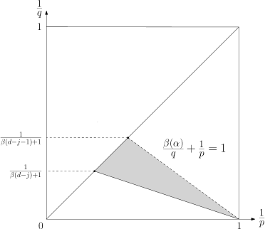
Figure 1. For $d-j-1<\alpha\leq d-j$, the edge line ${\beta(\alpha)}/{q}+{1}/{p}=1$ is contained in the shaded area. The region given by ${\beta(\alpha)}/{q}+{1}/{p}<1$ gets larger as $\alpha$ decreases.

The following is our first result.

Theorem 1.1.

Let $\gamma\in C^{d+1}(I)$ and $0<\alpha\leq d$ and let $\mu$ be a positive Borel measure. Suppose that $\gamma$ and $\mu$ satisfy (2) and (4), respectively. Then, for $1\leq p,q\leq\infty$ satisfying $d/{q}\leq(1-1/p)$, $q\geq 2d$, and

$$\beta(\alpha)/q+1/p<1,\,\,q>\beta(\alpha)+1,$$

there exists a constant $C$ such that (5) holds for $f\in L^{p}(I)$ and $\lambda\geq 1$.

As $\alpha$ decreases the admissible range of $p,q$ gets larger (see Figure 1). If $\alpha=d$, this extends Drury’s result [16] to general measures except for the end line case $\beta(d)/q+1/p=1$. (Note that $\beta(d)=(d^{2}+d)/2$.) The condition $d/{q}\leq(1-1/p)$, $q\geq 2d$ is related to application of Plancherel’s theorem which gives $d$-linear estimates (see Lemma 2.5). The condition $\beta(\alpha)/q+1/p<1$ is sharp in that there is a measure satisfying (4) but (5) fails if $\beta(\alpha)/q+1/p>1$ (see Appendix A). The restriction $q>\beta(\alpha)+1$ also seems necessary in general even though at present we know it only in special cases. Note that $\beta(\alpha)>d$ if $\alpha>1$ and $\beta(\alpha)+1>2d$ if $\alpha>2$. Hence, the assumption $d/{q}\leq(1-1/p)$, $q\geq 2d$ is redundant when $\alpha>2$. In particular, when $\mu$ is the surface measure on a compact smooth hypersurface $\Sigma\subset\mathbb{R}^{d}$ and $d\geq 3$, by rescaling the estimate (5) we get

$$\|T_{1}f\|_{L^{q}(\lambda\Sigma)}\leq C\|f\|_{L^{p}(I)}$$

provided that $(d+2)(d-1)/(2q)+1/p<1$ and $p\leq q$. This can be seen as a generalization of $L^{p}(S^{1})$-$L^{q}(\lambda S^{1})$ bound [9] (also see [22] and [4] for related results) for the extension operator from the circle $S^{1}$ in $\mathbb{R}^{2}$ to the large circle $\lambda S^{1}$.

Our results here rely on the so-called multilinear approach which has been used to study the restriction problem for hypersurfaces (cf. [2, 28]). Especially we adapt the recent argument due to Bourgain and Guth [10] (also see references therein) which was successful in deducing linear estimate from multilinear one. For the space curves with non vanishing torsion the sharp $d-$linear (extension) estimate is a straightforward consequence of Plancherel’s theorem under the assumption that the support functions are separated (see Lemma 2.5 and Lemma 2.6). Then it is crucial to control $T_{\lambda}f$ by products of $T_{\lambda}f_{1},\dots,T_{\lambda}f_{d}$ for which the supports of $f_{i}$ are separated from one another while the remaining parts are bounded by a sum of $|T_{\lambda}g|$ with $g$ supported in a small interval. (See Lemma 2.8.) Compared with [10] this is relatively simpler since we only have to deal with one parameter separation in order to make use of the multilinear estimate. To close induction we need to obtain uniform estimates which do not depend on particular choices of curves. After proper normalization we can reduce the matter to dealing with a class of curves which are close to a monomial curve. An obvious byproduct of this approach is stability of estimates over a family of curves (see Remark 2.9).

The estimates of the endpoint line case ($\beta(\alpha)/q+1/p=1$) are not likely to be possible with general measures satisfying (4). But they still look plausible with specific measures which satisfy certain regularity assumptions. However, these endpoint estimates are beyond the method of this paper. On the other hand, one may try to use the method based on offspring curves [16] but a routine adaptation of the presently known argument only gives (5) on a smaller range, namely $d/{q}\leq(1-1/p)$, $q\geq 2d$, $\beta(d)/q+1/p<1$ and $q>\beta(d)+1$.

Finite type curves

There are also results when curves degenerate, namely the condition (2) fails. Let us set $\mathbf{a}=(a_{1},\cdots,a_{d})$ with positive integers $a_{1},a_{2},\cdots,a_{d}$ satisfying $a_{1}<a_{2}<\cdots<a_{d}$. Then for $t\in I$ we also set

(6) $$M_{t}^{\gamma,\mathbf{a}}=\begin{bmatrix}\gamma^{(a_{1})}(t),&\gamma^{(a_{2})}(t),&\cdots,&\gamma^{(a_{d})}(t)\end{bmatrix},$$

where the column vectors $\gamma^{(a_{i})}(t)$ are $a_{i}$–th derivatives of $\gamma$. So, $\gamma$ is nondegenerate at $t$ if $\det M_{t}^{\gamma,\mathbf{a}}\neq 0$ with $\mathbf{a}=(1,2,\cdots,d)$. We recall the following definition which was introduced in [11].

Definition 1.2.

Let $\gamma:I=[0,1]\to\mathbb{R}^{d},\,d\geq 2$ be a smooth curve. We say that $\gamma$ is of finite type at $t\in I$ if there exists $\mathbf{a}=(a_{1},\cdots,a_{d})$ such that $\det M_{t}^{\gamma,\mathbf{a}}\neq 0$. We also say that $\gamma$ is of finite type if so is $\gamma$ at every $t\in I$.

When degeneracy appears the boundedness of $T_{\lambda}^{\gamma}$ is no longer the same so that (5) holds only on a smaller set of $p,q$. When $\mu$ is the Lebesgue measure Christ [11] obtained some sharp restriction estimates for the curves of finite type on a restricted range. On the other hand, a natural attempt is to recover the full range (3) by introducing a weight which mitigates bad behavior at degeneracy. In fact, let us consider the estimate

$$\|T_{\lambda}^{\gamma}[w,f]\|_{L^{q}(d\mu)}\leq C\lambda^{-\frac{\alpha}{q}}\|f\|_{L^{p}(wdt)},$$

where $\lambda\geq 1$ and

$$T_{\lambda}^{\gamma}[w,f](x)=\int_{I}e^{i\lambda x\cdot\gamma(t)}f(t)w(t)dt.$$

The dual form of this estimate with $\lambda=1$ is

(7) $$\Big{(}\int_{I}|\widehat{gd\mu}(\gamma(t))|^{p^{\prime}}w(t)dt\Big{)}^{1/p^{\prime}}\leq C\|g\|_{L^{q^{\prime}}(d\mu)}.$$

There has been a long line of investigations on the estimate (7) [18, 19, 17, 5, 7, 6, 8, 15, 14] when $\mu$ is the Lebesgue measure and $wdt$ is the affine arclength measure. When $d=2$, it was shown by Sjölin [26] (also see [24]). In higher dimensions the study on (7) was carried out by Drury and Marshall [18], [19]. Drury [17], Bak and Oberlin [5] obtained partial results for specific classes of curves in $\mathbb{R}^{3}$. If $I=\mathbb{R}$, by scaling the condition ${d(d+1)}/(2p^{\prime})=1/q$ is necessary for (7). Wright and Dendrinos [15] obtained a uniform estimate for a class of polynomial curves on the range $(d^{2}+2d)/2<q\leq\infty$. This result was extended to a larger region [8] (see Section 8). There is also a result for the curves of which components are rational functions rather than polynomials (see [12]). Bak, Oberlin and Seeger obtained the estimates on the full range including the weak endpoint estimate for the monomial curves and the curves of simple type [8]. Dendrinos and Müller [14] further extended this result to the curves of small perturbation of monomial curves and for the critical case $p=q={(d^{2}+d+2)/2}$ the weak type endpoint estimate also holds for these curves (see Remark in Section 6 of [8]). The problem of obtaining (7) is now settled for the finite type curves which are defined locally though the uniform estimate is still open when curves are given on the whole real line.

In what follows we consider $L^{p}$–$L^{q}$ estimate of $T_{\lambda}^{\gamma}[w_{\gamma}^{\alpha},f]$ with respect to the measure $\mu$ satisfying (4). Let us define a measure by setting

$$w_{\gamma}^{\alpha}(t)dt=|\det(\gamma^{\prime}(t),\gamma^{\prime\prime}(t),\cdots,\gamma^{(d)}(t))|^{\frac{1}{\beta(\alpha)}}dt.$$

When $\alpha=d$ this coincides with the affine arclength measure on $\gamma$. Considering a monomial curve and a measure satisfying the homogeneity condition $\int g(\lambda x)d\mu(x)=\lambda^{-\alpha}\int g(x)d\mu(x)$ (for example the measure $\mu$ given in Appendix A), by rescaling one can easily see that the exponent $1/\beta(\alpha)$ is the correct choice in order that the estimate (8) holds for $p,q$ satisfying $\beta(\alpha)/q+1/p\leq 1$. In [8] (see Section 2), when $\mu$ is the Lebesgue measure it was shown that the optimal power of torsion is $1/\beta(d)=2/d(d+1)$ so that (7) holds for $d(d+1)/(2q)+1/p\leq 1$. If we consider the induced Lebesgue measure on lower dimensional hyperplanes, this clearly shows that our choice of $\beta(\alpha)$ is optimal at least if $\alpha$ is an integer.

Our second result reads as follows.

Theorem 1.3.

Let $\gamma\in C^{\infty}(I)$ and $0<\alpha\leq d$. Suppose that $\mu$ satisfies (4) and $\gamma$ is of finite type. Then, for $1\leq p,q\leq\infty$ satisfying $d/{q}\leq(1-1/p)$, $q\geq 2d$ and $\beta(\alpha)/q+1/p<1$, $q>\beta(\alpha)+1$, there exists a constant $C$ such that

(8) $$\|T_{\lambda}^{\gamma}[w_{\gamma}^{\alpha},f]\|_{L^{q}(d\mu)}\leq C\lambda^{-\frac{\alpha}{q}}\|f\|_{L^{p}(w_{\gamma}^{\alpha}dt)}.$$

This generalizes the previous results to general measures except for $p,q$ which are on the end line. Thanks to the finite type assumption a suitable normalization by a finite decomposition and rescaling reduce the problem to the case of monomial type curves of which degeneracy only appears a single point. Further decomposition away from the degeneracy enables us to obtain the desired estimate (8) by relying on the stability of estimates for non-degenerate curves.

The paper is organized as follows. In Section 2 we prove Theorem 1.1. In Section 3 we give the proof of Theorem 1.3 which is based on Theorem 1.1. Sharpness of the condition $\beta(\alpha)/q+1/p<1$ will be shown in Appendix A.

2. Proof of Theorem 1.1

The proof of Theorem 1.1 is based on an adaptation of Bourgain-Guth argument in [10], which relies on a multilinear estimate and uniform control of estimates over classes of curves and measures. This requires proper normalization of them.

Normalization of curves

For $a,b\in\mathbb{R}$, $a\neq b$, we set

$$[a,b]^{*}=\begin{cases}\,\,[a,b]\,\,\text{ if }a<b,\\ \,\,[b,a]\,\,\text{ if }b<a.\end{cases}$$

Let $\gamma\in C^{d+1}(I)$ satisfying (2), and let $\tau\in I$ and $h$ be a real number such that $[\tau,\tau+h]^{*}\subset I$. Then let us define a $d\times d$ matrix $M_{\tau}^{\gamma}$ and a diagonal matrix $D_{h}$ by

$$M_{\tau}^{\gamma} =M_{\tau}^{\gamma,(1,2,\dots,d)}=(\gamma^{\prime}(\tau),\gamma^{\prime\prime}(\tau),\cdots,\gamma^{(d)}(\tau)),$$

$$\quad D_{h} =(he_{1},h^{2}e_{2},\dots,h^{d}e_{d}).$$

We also set

(9) $$\gamma_{\tau}^{h}(t)=D_{h}^{-1}(M_{\tau}^{\gamma})^{-1}(\gamma(ht+\tau)-\gamma(\tau)).$$

Then it follows that

(10) $$x\cdot(\gamma(ht+\tau)-\gamma(\tau))=D_{h}(M_{\tau}^{\gamma})^{t}x\cdot\gamma_{\tau}^{h}(t).$$

Let us set

$$\gamma_{\circ}(t)=\Big{(}t,\frac{t^{2}}{2!},\dots,\frac{t^{d}}{d!}\,\Big{)}.$$

For a given $\epsilon>0$ we define the class $\mathfrak{G}(\epsilon)$ of curves by setting

$$\mathfrak{G}(\epsilon)=\Big{\{}\gamma\in C^{d+1}(I):\|\gamma-\gamma_{\circ}\|_{C^{d+1}(I)}\leq\epsilon\Big{\}}.$$

Lemma 2.1.

Let $\gamma\in C^{d+1}(I)$ satisfying (2) and let $\tau\in I$. Then, for $\epsilon>0$ there is a constant $\delta>0$ such that $\gamma_{\tau}^{h}\in\mathfrak{G}(\epsilon)$ whenever $[\tau,\tau+h]^{*}\subset I$ and $0<|h|\leq\delta$.

For a given matrix $M$, $\|M\|$ denotes the usual matrix norm $\max_{|x|=1}|Mx|$.

Proof.

It is enough to consider the case $[\tau,\tau+h]\subset I$. The other case $[h+\tau,\tau]\subset I$ can be shown similarly. By Taylor’s expansion

$$\gamma(ht+\tau)-\gamma(\tau) =\gamma^{{}^{\prime}}\!(\tau)ht+\gamma^{{}^{\prime\prime}}\!(\tau)h^{2}\frac{t^{2}}{2!}+\dots+\gamma^{(d)}\!(\tau)h^{d}\frac{t^{d}}{d!}+\mathcal{E}(\tau,h,t)$$

$$=M_{\tau}^{\gamma}D_{h}\gamma_{\circ}(t)+\mathcal{E}(\tau,h,t)$$

with $\|\mathcal{E}(\tau,h,t)\|_{C^{d+1}(I)}\leq Ch^{d+1}$ uniformly in $\tau$. Since $\gamma_{\tau}^{h}(t)=\gamma_{\circ}(t)+(M_{\tau}^{\gamma}D_{h})^{-1}$ $\mathcal{E}(\tau,h,t),$

(11) $$\|\gamma_{\tau}^{h}-\gamma_{\circ}\|_{C^{d+1}(I)}\leq C\|(M_{\tau}^{\gamma})^{-1}\|h.$$

By continuity $\|(M_{\tau}^{\gamma})^{-1}\|$ is uniformly bounded along $\tau\in I$ by a constant $B$ because $\gamma$ satisfies (2) and $\gamma\in C^{d+1}(I)$. Taking $\delta=\epsilon/(2CB)$, we see $\gamma_{\tau}^{h}\in\mathfrak{G}(\epsilon)$. ∎

Remark 2.2.

Let $J\subset I$. From the proof of Lemma 2.1 it is clear that if $\|\gamma\|_{C^{d+1}(J)}\leq B_{1}$ and $\|(M_{\tau}^{\gamma})^{-1}\|\leq B_{2}$ for all $\tau\in J$, then for $\epsilon>0$ there is a $\delta=\delta(B_{1},B_{2})>0$ such that $\gamma_{\tau}^{h}\in\mathfrak{G}(\epsilon)$ provided that $[\tau,\tau+h]^{*}\subset J$ and $0<|h|\leq\delta$.

Rescaling of measures

For $M>0$ we denote by $\mathfrak{B}(\alpha,M)$ the set of positive Borel measures which satisfy (4) with $C_{\mu}=M$. If $\sigma\in\mathfrak{B}(\alpha,M)$, $\sigma$ is finite on all compact sets in $\mathbb{R}^{d}$ by $\eqref{bmeasure}$. Hence, $\sigma$ is a Radon measure because $\mathbb{R}^{d}$ is locally compact Hausdorff space. (See Theorem 7.8 in [21].)

For $\mathbf{a}=(a_{1},\cdots,a_{d})$ let us define

(12) $$D_{h}^{\mathbf{a}}=(h^{a_{1}}e_{1},h^{a_{2}}e_{2},\dots,h^{a_{d}}e_{d}).$$

Let $\sigma\in\mathfrak{B}(\alpha,M)$, $0<|h|<1$, and let $A$ be a $d\times d$ nonsingular matrix. Then the map $F\to\int F(D_{h}^{\mathbf{a}}A\,x)d\sigma(x)$ defines a positive linear functional on $C_{c}(\mathbb{R}^{d})$. By the Riesz representation theorem there exists a unique Radon measure $\sigma_{\!A,h}^{\mathbf{a}}$ such that

(13) $$\int F(x)d\sigma_{\!A,h}^{\mathbf{a}}(x)=\int F(D_{h}^{\mathbf{a}}A\,x)d\sigma(x)$$

for any compactly supported continuous function $F$.

Lemma 2.3.

Let  $\mathbf{a}=(a_{1},\dots,a_{d})$ and $a_{1},a_{2},\dots,a_{d}$ satisfy that $0<a_{1}<a_{2}<\ldots<a_{d}$ and $a_{i}\geq i$. If $\sigma\in\mathcal{B}(\alpha,M)$ and $A$ is a nonsingular matrix, then $\sigma_{\!A,h}^{\mathbf{a}}$ is also a Borel measure which satisfies

(14) $$\sigma_{\!A,h}^{\mathbf{a}}(B(x,\rho))\leq CM\|A^{-1}\|^{\alpha}|h|^{\frac{d^{2}+d}{2}-\beta(\alpha)-\sum_{i=1}^{d}a_{i}}\rho^{\alpha}$$

for $(x,\rho)\in\mathbb{R}^{d}\times\mathbb{R}_{+}$. Here $C$ is independent of $h,A$.

Proof.

Let $d-j-1<\alpha\leq d-j$ for some $j=0,\dots,d-1$. By translation we may assume $x=0$. To show (14), we consider $\sigma_{\!A,h}^{\mathbf{a}}$ as a measure which is given by composition of two transformations on $\sigma$.

We first consider the measure $\sigma_{A}$ defined by

$$\int F(x)d\sigma_{A}=\int F(Ax)d\sigma(x),\quad F\in C_{c}(\mathbb{R}^{d})$$

with a nonsingular matrix $A$. Then it follows that

$$\sigma_{A}(B(0,\rho))\leq M\|\omega\|^{\alpha}\rho^{\alpha},$$

where $\|\omega\|=\max_{k}|\omega_{k}|$ and $\omega_{1},\dots,\omega_{d}$ are the column vectors of $A^{-1}$. In fact, $Ax\in B(0,\rho)$ implies that $x$ can be written as a linear combination of $\omega_{k}$ with a coefficient vector in $B(0,\rho)$, i.e. $x=z_{1}w_{1}+\cdots+z_{d}\omega_{d}$ with $(z_{1},\dots,z_{d})\in B(0,\rho)$. Since $\sigma\in\mathfrak{B}(\alpha,M)$, we have

(15) $$\sigma_{A}(B(0,\rho))=\int\chi_{B(0,\rho)}(Ax)d\sigma(x)\leq C\int\chi_{B(0,d\|\omega\|\rho)}(y)d\sigma(y)\leq CM(\|\omega\|\rho)^{\alpha}.$$

Let us define a measure $\sigma_{h}^{\mathbf{a}}$ by

$$\int F(x)d\sigma_{h}^{\mathbf{a}}=\int F(D_{h}^{\mathbf{a}}x)d\sigma,$$

and claim that

(16) $$\sigma_{h}^{\mathbf{a}}(B(0,\rho))\leq CM|h|^{\frac{d^{2}+d}{2}-\sum_{i=1}^{d}a_{i}-\beta(\alpha)}\rho^{\alpha}.$$

Since $\{x:Ax\in B(0,\rho)\}\subset B(0,d\|\omega\|\rho)$, by (15) and (16) it follows that

$$\sigma_{\!A,h}^{\mathbf{a}}(B(0,\rho)) =\int\chi_{B(0,\rho)}(Ax)d\sigma_{h}^{\mathbf{a}}(x)\leq C\sigma_{h}^{\mathbf{a}}(B(0,d\|\omega\|\rho))$$

$$\leq CM\|\omega\|^{\alpha}|h|^{\frac{d^{2}+d}{2}-\sum_{i=1}^{d}a_{i}-\beta(\alpha)}\rho^{\alpha},$$

and therefore we get (14).

Now it remains to show (16). Let us set

$$S=\{y:D_{h}^{\mathbf{a}}y\in B(0,\rho)\}.$$

Then, if $y=(y_{1},\dots,y_{d})\in S$ we have $|y_{i}|\leq|h|^{-a_{i}}\rho$. Hence, $S$ is contained in the rectangle $\mathcal{R}$ of dimension $|h|^{-a_{1}}\rho\times|h|^{-a_{2}}\rho\times\cdots\times|h|^{-a_{d}}\rho$. So, $\mathcal{R}$ can be covered by as many as $O(|h|^{-a_{1}+1}\times|h|^{-a_{2}+2}\times\cdots\times|h|^{-a_{d}+d})$ rectangles $\mathcal{R}^{\prime}$ of which dimension is $|h|^{-1}\rho\times|h|^{-2}\rho\times\dots\times|h|^{-d}$ while each $\mathcal{R}^{\prime}$ is covered by $O(1\times\cdots\times 1\times|h|^{-1}\times\cdots\times|h|^{-(d-j-1)})$ cubes of sidelength $|h|^{-j-1}\rho$. Hence $\mathcal{R}$ is covered by cubes $\mathcal{B}_{1},\dots,\mathcal{B}_{l}$ of sidelength $|h|^{-j-1}\rho$ with $l\lesssim|h|^{(\frac{d^{2}+d}{2}-\sum_{i=1}^{d}a_{i}-\frac{(d-j-1)(d-j)}{2})}$. Hence,

$$\sigma_{h}^{\mathbf{a}}(B(0,\rho))\leq\int\chi_{B(0,\rho)}(D_{h}^{\mathbf{a}}y)d\sigma(y)\leq\int\chi_{\mathcal{R}}(y)d\sigma(y)$$

$$\leq\sum_{i=1}^{l}\int\chi_{\mathcal{B}_{i}}(y)d\sigma(y)=\sum_{i=1}^{l}\sigma(\mathcal{B}_{i})\lesssim M\sum_{i=1}^{l}|h|^{-(j+1)\alpha}\rho^{\alpha}$$

$$\leq CM|h|^{(\frac{d^{2}+d}{2}-\sum_{i=1}^{d}a_{i}-\frac{(d-j-1)(d-j)}{2}-(j+1)\alpha)}\rho^{\alpha}.$$

This gives the desired inequality since $(j+1)\alpha+{(d-j-1)(d-j)}/{2}=\beta(\alpha)$. ∎

Multilinear $(d-linear)$ estimates with separated supports

We now prove a multilinear estimate with respect to general measures, which is basically a consequence of Plancherel’s theorem. We also show that the estimates are uniform along $\gamma\in\mathfrak{G}(\epsilon)$ if $\epsilon>0$ is small enough.

Let us define a map $\Gamma_{\gamma}:I^{d}\to\mathbb{R}^{d}$ by

$$\Gamma_{\gamma}(\mathbf{t})=\sum_{i=1}^{d}\gamma(t_{i}),$$

where $\mathbf{t}=(t_{1},t_{2},\cdots,t_{d})$.

Lemma 2.4.

Let $E=\{\mathbf{t}\in I^{d}:\,t_{1}<t_{2}<\ldots<t_{d}\}$. If $\epsilon>0$ is sufficiently small, then the map $\mathbf{t}:E\to\Gamma_{\gamma}(\mathbf{t})$ is one to one for all $\gamma\in\mathfrak{G}(\epsilon)$.

This can be shown by the argument in [19] which relies on total positivity (also see [15]). In fact, we need to show that total positivity is valid on $I$ regardless of $\gamma\in\mathfrak{G}(\epsilon)$. It is not difficult by making use of the fact that $\gamma$ is a small perturbation of $\gamma_{\circ}$. We give a proof of Lemma 2.4 in Appendix B.

Now, the following is a straightforward consequence of Plancherel’s theorem.

Lemma 2.5.

Let $\gamma\in\mathfrak{G}(\epsilon)$ and $\mathcal{I}_{1},\dots,\mathcal{I}_{d}$ be closed intervals contained in $I$ which satisfy $\min_{i\neq j}\operatorname{dist}(\mathcal{I}_{i},\mathcal{I}_{j})\geq L>0$. If $\epsilon>0$ is sufficiently small, then there is a constant $C$, independent of $\gamma$, such that

$$\|\prod_{i=1}^{d}T_{\lambda}^{\gamma}f_{i}\|_{L^{2}}\leq CL^{-\frac{d^{2}-d}{4}}\lambda^{-\frac{d}{2}}\prod_{i=1}^{d}\|f_{i}\|_{L^{2}}$$

whenever $f_{i}$ is supported in $\mathcal{I}_{i}$, $i=1,2,\dots,d$.

Proof.

Let $f_{1},\dots,f_{d}$ be supported in each interval $\mathcal{I}_{i}$, $i=1,2,\dots,d$, and set $F(\mathbf{t})=\prod_{i=1}^{d}f_{i}(t_{i})\chi_{\mathcal{I}_{i}}(t_{i})$. Then, by Lemma 2.4 $\Gamma_{\gamma}:\prod_{i=1}^{d}\mathcal{I}_{i}\to\mathbb{R}^{d}$ is one to one. Hence by the change of variables $y=\Gamma_{\gamma}(\mathbf{t})$, we have

$$\prod_{i=1}^{d}T_{\lambda}^{\gamma}f_{i}=\int_{I^{d}}e^{i\lambda x\cdot\Gamma_{\gamma}(\mathbf{t})}F(\mathbf{t})d\mathbf{t}=\widehat{G}(\lambda x),$$

where $G(y)=F(\mathbf{t}(y))|\det\big{(}\frac{\partial\Gamma_{\gamma}}{\partial\mathbf{t}}\big{)}(\mathbf{t}(y))|^{-1}$. By Plancherel’s theorem and reversing the change of variables $y\mapsto\mathbf{t}$, we see

$$\|\prod_{i=1}^{d}T_{\lambda}^{\gamma}f_{i}\|_{L^{2}(\mathbb{R}^{d})} =\lambda^{-\frac{d}{2}}\|G\|_{L^{2}(\mathbb{R}^{d})}=\lambda^{-\frac{d}{2}}\bigg{(}\int|F(\mathbf{t})|^{2}\Big{|}\det\Big{(}\frac{\partial\Gamma_{\gamma}}{\partial\mathbf{t}}\Big{)}\Big{|}^{-1}d\mathbf{t}\bigg{)}^{\frac{1}{2}}.$$

Since $|t_{j}-t_{i}|\geq L$, $i\neq j$, it is sufficient to show that for all $\gamma\in\mathfrak{G}(\epsilon)$

$$\Big{|}\det\Big{(}\frac{\partial\Gamma_{\gamma}}{\partial\mathbf{t}}\Big{)}\Big{|}\geq\frac{1}{2\prod_{i=1}^{d}(i-1)!}\prod_{1\leq i<j\leq d}|t_{j}-t_{i}|$$

if $\epsilon$ is sufficiently small. If $\gamma\in\mathfrak{G}(\epsilon)$, then $\gamma=\gamma_{\circ}+\mathcal{E}$ and $\|\mathcal{E}\|_{C^{d+1}(I)}\leq\epsilon$. Hence by a computation with a generalized mean value theorem we see that

$$\Big{|}\det\Big{(}\frac{\partial\Gamma_{\gamma}}{\partial\mathbf{t}}\Big{)}\Big{|}\geq\frac{1}{\prod_{i=1}^{d}(i-1)!}\prod_{1\leq i<j\leq d}|t_{j}-t_{i}|\,\times(1-\epsilon 2^{d-1}d!).$$

Taking a small $\epsilon$ so that $\epsilon<(2^{d}d!)^{-1}$, we get the desired estimate. This completes proof. ∎

Using Lemma 2.5, we obtain the following $L^{p}$–$L^{q}$ estimate via interpolation with $L^{1}$–$L^{\infty}$ estimate.

Proposition 2.6.

Let $\mathcal{I}_{1},\dots,\mathcal{I}_{d}$, and $\gamma\in\mathfrak{G}(\epsilon)$ be given as in Lemma 2.5. Suppose $\mu$ satisfies (4). If $\epsilon>0$ is sufficiently small, then for $1/p+1/q\leq 1$ and $q\geq 2$ there is a constant $C$, independent of $\gamma$, such that

$$\|\prod_{i=1}^{d}T_{\lambda}^{\gamma}f_{i}\|_{L^{q}(d\mu)}\leq CC_{\mu}^{\frac{1}{q}}L^{-\frac{d^{2}-d}{2q}}\lambda^{-\frac{\alpha}{q}}\prod_{i=1}^{d}\|f_{i}\|_{p}$$

whenever $f_{i}$ is supported in $\mathcal{I}_{i}$, $i=1,2,\dots,d$.

Proof.

To begin with, we observe that the trivial $L^{1}$–$L^{\infty}$ estimate

$$\|\prod_{i=1}^{d}T_{\lambda}^{\gamma}f_{i}\|_{L^{\infty}(d\mu)}\leq\prod_{i=1}^{d}\|f_{i}\|_{1}$$

holds. It is obvious because $\prod_{i=1}^{d}T_{\lambda}^{\gamma}f_{i}$ is continuous and $|\prod_{i=1}^{d}T_{\lambda}^{\gamma}f_{i}|\leq\prod_{i=1}^{d}\|f_{i}\|_{1}$. Since $f_{i}$ is supported in $\mathcal{I}_{i}\subset I$, by Hölder’s inequality and interpolation, it suffices to show that

(17) $$\|\prod_{i=1}^{d}T_{\lambda}^{\gamma}f_{i}\|_{L^{2}(d\mu)}\leq CC_{\mu}^{\frac{1}{2}}L^{-\frac{d^{2}-d}{4}}\lambda^{-\frac{\alpha}{2}}\prod_{i=1}^{d}\|f_{i}\|_{2}.$$

Note that the Fourier transform $\mathcal{F}({\prod_{i=1}^{d}T_{\lambda}^{\gamma}f_{i}})$ of $\prod_{i=1}^{d}T_{\lambda}^{\gamma}f_{i}$ is supported in a ball of radius $C\sqrt{2d}\,\lambda$ for some $C>0$. Let $\varphi$ be a smooth function such that $\widehat{\varphi}=0$ if $|\xi|\geq 2C\sqrt{2d}$ and $\widehat{\varphi}=1$ if $|\xi|\leq C\sqrt{2d}$. Then, $\mathcal{F}({\prod_{i=1}^{d}T_{\lambda}^{\gamma}f_{i}})(\xi)=\mathcal{F}({\prod_{i=1}^{d}T_{\lambda}^{\gamma}f_{i}})(\xi){\widehat{\varphi}}(\xi/\lambda)$. Hence $\prod_{i=1}^{d}T_{\lambda}^{\gamma}f_{i}=\varphi_{\lambda}\ast(\prod_{i=1}^{d}T_{\lambda}^{\gamma}f_{i})$ where $\varphi_{\lambda}(x)=\lambda^{d}\varphi(\lambda x)$. This and Hölder’s inequality gives

$$|\prod_{i=1}^{d}T_{\lambda}^{\gamma}f_{i}|^{2}\leq C|\prod_{i=1}^{d}T_{\lambda}^{\gamma}f_{i}|^{2}\ast|\varphi|_{\lambda}$$

with $C$ only depending on $\varphi$. By the rapid decay of $\varphi$ and (4), it follows that

$$|\varphi_{\lambda}|\ast\mu=\int\lambda^{d}|\varphi|(\lambda(x-y))d\mu(y)\leq CC_{\mu}\lambda^{d-\alpha}.$$

Therefore, this and Fubini’s theorem give

$$\|\prod_{i=1}^{d}T_{\lambda}^{\gamma}f_{i}\|_{L^{2}(d\mu)} \leq\Big{(}\int|\prod_{i=1}^{d}T_{\lambda}^{\gamma}f_{i}|^{2}\ast|\varphi|_{\lambda}d\mu(x)\Big{)}^{\frac{1}{2}}\leq\|\prod_{i=1}^{d}T_{\lambda}f_{i}\|_{2}\,\||\varphi|_{\lambda}\ast\mu\|_{\infty}^{\frac{1}{2}}$$

$$\lesssim C_{\mu}^{\frac{1}{2}}L^{-\frac{d^{2}-d}{4}}\lambda^{-\frac{d}{2}}\lambda^{\frac{d}{2}-\frac{\alpha}{2}}\prod_{i=1}^{d}\|f_{i}\|_{2}\lesssim C_{\mu}^{\frac{1}{2}}L^{-\frac{d^{2}-d}{4}}\lambda^{-\frac{\alpha}{2}}\prod_{i=1}^{d}\|f_{i}\|_{2}.$$

For the third inequality we use Lemma 2.5. Hence we get (17). ∎

Induction quantity

For $1\leq\lambda,$ $1\leq p,q\leq\infty$, and $\epsilon>0$, we define $Q_{\lambda}(R)=Q_{\lambda}(R,p,q,\epsilon)$ by setting

(18) $$Q_{\lambda}(R)=\sup\{\,\,\|T_{\lambda}^{\gamma}f\|_{L^{q}(d\mu,B_{R})}:\mu\in\mathfrak{B}(\alpha,1),\,\gamma\in\mathfrak{G}(\epsilon),\,{\|f\|_{L^{p}(I)}\leq 1}\}$$

where $B_{R}$ is the open ball of radius $R$ centred at the origin. Clearly, $Q_{\lambda}(R)<\infty$ because $Q_{\lambda}(R)\leq R^{\alpha/q}$ for any $\lambda>0$.

Lemma 2.7.

Let $\gamma\in\mathfrak{G}(\epsilon)$, $\mu\in\mathfrak{B}(\alpha,1)$, and let $\lambda\geq 1$, $0<|h|<1$. Suppose that $f$ is supported in the interval $[\tau,\tau+h]^{*}\subset[0,1]$. Then, if $\epsilon>0$ is sufficiently small, there is a constant $\delta>0$, independent of $\gamma$, such that if $0<|h|\leq\delta$

(19) $$\|T_{\lambda}^{\gamma}f\|_{L^{q}(d\mu,B_{R})}\leq C\,|h|^{1-\frac{1}{p}-\frac{\beta(\alpha)}{q}}Q_{\lambda}(R)\|f\|_{p}.$$

Proof.

We begin with setting $f_{h}=|h|f(ht+\tau)$. By translation, scaling and using (10) it follows that

(20) $$\begin{aligned} |T_{\lambda}^{\gamma}f(x)|=\bigg{|}\int_{I}e^{i\lambda x\cdot(\gamma(ht+\tau)-\gamma(\tau))}f_{h}(t)dt\bigg{|}=\bigg{|}\int_{I}e^{i\lambda D_{h}(M_{\tau}^{\gamma})^{t}x\cdot\gamma_{\tau}^{h}(t)}f_{h}(t)dt\bigg{|}.\end{aligned}$$

We denote by $\mu_{\tau}^{h}$ the measure given by

(21) $$\int F(x)d\mu_{\tau}^{h}(x)=\int F(D_{h}(M_{\tau}^{\gamma})^{t}x)d\mu(x)$$

and set

$$d\widetilde{\mu}(x)=\frac{|h|^{\beta(\alpha)}}{1+C\|(M_{\tau}^{\gamma})^{-t}\|^{\alpha}}\,d\mu_{\tau}^{h}(x).$$

Hence, we have

$$\int_{B_{R}}|T_{\lambda}^{\gamma}f(x)|^{q}d\mu(x)=\int|T_{\lambda}^{\gamma_{\tau}^{h}}f_{h}(x)|^{q}\chi_{B_{R}}((M_{\tau}^{\gamma})^{-t}D_{h}^{-1}x)d\mu_{\tau}^{h}(x)$$

$$= (1+C\|(M_{\tau}^{\gamma})^{-t}\|^{\alpha})|h|^{-\beta(\alpha)}\int|T_{\lambda}^{\gamma_{\tau}^{h}}f_{h}(x)|^{q}\chi_{B_{R}}((M_{\tau}^{\gamma})^{-t}D_{h}^{-1}x)d\widetilde{\mu}(x){\color[rgb]{1,0,0}.}$$

Now we note that $\|(M^{\gamma}_{\tau})^{-t}\|\leq C$ uniformly for $\gamma\in\mathfrak{G}(\epsilon)$ if $\epsilon>0$ is small enough. By Lemma 2.3  $\widetilde{\mu}\in\mathfrak{B}(\alpha,1)$, and $\gamma_{\tau}^{h}\in\mathfrak{G}(C|h|\epsilon)\subset\mathfrak{G}(\epsilon)$ if $0<|h|\leq\delta$  for a sufficiently small $\delta>0$. Moreover, the set $\{M^{\gamma}_{\tau}D_{h}x:x\in B_{R}\}$ is also contained in $B_{R}$ for all $\gamma\in\mathfrak{G}(\epsilon)$ if $0<|h|\leq\delta$ and $\delta$ is small enough. Therefore, by the definition of $Q_{\lambda}(R)$ we see

$$\int_{B_{R}}|T_{\lambda}^{\gamma}f(x)|^{q}d\mu(x) \leq C|h|^{-\beta(\alpha)}\int_{B_{R}}|T_{\lambda}^{\gamma_{\tau}^{h}}f_{h}(x)|^{q}d\widetilde{\mu}(x)$$

$$\leq C|h|^{-\beta(\alpha)}(Q_{\lambda}(R)\,\|f_{h}\|_{p})^{q}$$

$$=C|h|^{-\beta(\alpha)+q-\frac{q}{p}}(Q_{\lambda}(R)\|f\|_{p})^{q}.$$

This gives the desired inequality (19). ∎

Multilinear decomposition

Now we make a decomposition of $T_{\lambda}^{\gamma}$ which is needed to exploit the $d$-linear estimate with separated supports. This decomposition doesn’t depend on particular choices of $\gamma$.

Let $A_{1},\dots,A_{d-1}$ be dyadic numbers such that

$$1=A_{0}\gg A_{1}\gg A_{2}\dots\gg A_{d-1}.$$

For $i=1,\dots,d-1$, let us denote by $\{\mathfrak{I}^{i}\}$ the collection of closed dyadic intervals of length $A_{i}$ which are contained in $[0,1]$. And we set

$$f_{\mathfrak{I}^{i}}=\chi_{\mathfrak{I}^{i}}f$$

so that for each $i=1,\dots,d-1,$ $f=\sum_{\mathfrak{I}^{i}}f_{\mathfrak{I}^{i}}$ almost everywhere whenever $f$ is supported in $I$. Hence, it follows that

(22) $$T_{\lambda}^{\gamma}f=\sum_{\mathfrak{I}^{i}}T_{\lambda}^{\gamma}f_{\mathfrak{I}^{i}},\,\,i=1,\dots,d-1.$$

Let $S_{1},\dots,S_{i}$ be subsets of $I$ and let us define

$$\Delta(S_{1},S_{2},\dots,S_{i})=\min_{j\neq k}\,\operatorname{dist}(S_{j},S_{k}).$$

Lemma 2.8.

Let $\gamma:I\to\mathbb{R}^{d}$ be a smooth curve. Let $A_{0},A_{1},\dots,A_{d-1}$, and $\{\mathfrak{I}^{i}\}$, $i=1,\dots,d-1$ be defined as in the above. Then, for any $x\in\mathbb{R}^{d}$, there is a constant $C$, independent of $\gamma,x$, $A_{0},A_{1},\dots,A_{d-1}$, such that

(23) $$|T_{\lambda}^{\gamma} f(x)|\leq\sum_{i=1}^{d-1}CA_{i-1}^{-2(i-1)}\max_{\mathfrak{I}^{i}}|T_{\lambda}^{\gamma}f_{\mathfrak{I}^{i}}(x)|$$

$$+CA_{d-1}^{-2(d-1)}\max_{\begin{subarray}{c}\mathfrak{I}^{d-1}_{1},\mathfrak{I}^{d-1}_{2},\dots,\mathfrak{I}^{d-1}_{d};\\ \Delta(\mathfrak{I}^{d-1}_{1},\mathfrak{I}^{d-1}_{2},\dots,\mathfrak{I}^{d-1}_{d})\geq A_{d-1}\end{subarray}}|\prod_{i=1}^{d}T_{\lambda}^{\gamma}f_{\mathfrak{I}^{d-1}_{i}}(x)|^{\frac{1}{d}}.$$

Here $\mathfrak{I}^{i}_{j}$ denotes the element in $\{\mathfrak{I}^{i}\}$.

The exact exponents of $A_{i}$ are not important for the argument below. So, we don’t try to obtain the best exponents.

Proof.

Fix $x\in\mathbb{R}^{d}$. By a simple argument it is easy to see that

(24) $$|T_{\lambda}^{\gamma}f(x)|\leq C\max_{\mathfrak{I}^{1}}|T_{\lambda}^{\gamma}f_{\mathfrak{I}^{1}}(x)|+CA_{1}^{-1}\max_{\begin{subarray}{c}\mathfrak{I}^{1}_{1},\mathfrak{I}^{1}_{2};\\ \Delta(\mathfrak{I}^{1}_{1},\mathfrak{I}^{1}_{2})\geq{A_{1}}\end{subarray}}|T_{\lambda}^{\gamma}f_{\mathfrak{I}^{1}_{1}}(x)T_{\lambda}^{\gamma}f_{\mathfrak{I}^{1}_{2}}(x)|^{\frac{1}{2}}.$$

Indeed, let $\mathfrak{I}^{1}_{\ast}\in\{\mathfrak{I}^{1}\}$ be the interval such that $|T_{\lambda}^{\gamma}f_{\mathfrak{I}^{1}_{\ast}}(x)|=\max_{\mathfrak{I}^{1}}|T_{\lambda}^{\gamma}f_{\mathfrak{I}^{1}}(x)|$. We now consider the cases $|T_{\lambda}^{\gamma}f(x)|\leq 100|T_{\lambda}^{\gamma}f_{\mathfrak{I}^{1}_{\ast}}(x)|,$ $|T_{\lambda}^{\gamma}f(x)|\geq 100|T_{\lambda}^{\gamma}f_{\mathfrak{I}^{1}_{\ast}}(x)|,$ separately. For the latter case, from (22) it is easy to see that there is an interval $\mathfrak{I}^{1}_{1}\in\{\mathfrak{I}^{1}\}$ such that $|T_{\lambda}^{\gamma}f(x)|\leq CA_{1}^{-1}|T_{\lambda}^{\gamma}{f_{\mathfrak{I}^{1}_{1}}}(x)|$ and $\Delta(\mathfrak{I}^{1}_{\ast},\mathfrak{I}^{1}_{1})\geq A_{1}$. Then it follows that

$$|T_{\lambda}^{\gamma}f(x)|\leq CA_{1}^{-1}|T_{\lambda}^{\gamma}{f_{\mathfrak{I}^{1}_{1}}}(x)T_{\lambda}^{\gamma}f_{\mathfrak{I}^{1}_{\ast}}(x)|^{\frac{1}{2}}.$$

Combining two cases we get the desired inequality (24), which is clearly independent of $x$ and $\gamma$.

Now, for $2\leq j\leq d$ we claim that

(25) $$\max_{\begin{subarray}{c}\mathfrak{I}^{j-1}_{1},\mathfrak{I}^{j-1}_{2},\dots,\mathfrak{I}^{j-1}_{j};\\ \Delta(\mathfrak{I}^{j-1}_{1},\mathfrak{I}^{j-1}_{2},\dots,\mathfrak{I}^{j-1}_{j})\geq{A_{j-1}}\end{subarray}}|\prod_{i=1}^{j}T_{\lambda}^{\gamma}f_{\mathfrak{I}^{j-1}_{i}}(x)|^{\frac{1}{j}}$$

$$\leq C\max_{\mathfrak{I}^{j}}|T_{\lambda}f_{\mathfrak{I}^{j}}(x)|+CA_{j}^{-2}\max_{\begin{subarray}{c}\mathfrak{I}^{j}_{1},\mathfrak{I}^{j}_{2},\dots,\mathfrak{I}^{j}_{j+1};\\ \Delta(\mathfrak{I}^{j}_{1},\mathfrak{I}^{j}_{2},\dots,\mathfrak{I}^{j}_{j+1})\geq{A_{j}}\end{subarray}}|\prod_{i=1}^{j+1}T_{\lambda}^{\gamma}f_{\mathfrak{I}^{j}_{i}}(x)|^{\frac{1}{j+1}}$$

holds with $C$, independent of $x,$ $\gamma$, and $A_{j-1},A_{j}$. This proves the desired inequality. In fact, starting from (24) and applying (25) successively to the product terms we see that

$$|T_{\lambda}^{\gamma} f(x)|\leq C\sum_{i=1}^{d-1}\Big{[}\prod_{k=1}^{i}A_{k-1}^{-2}\Big{]}\max_{\mathfrak{I}^{i}}|T_{\lambda}^{\gamma}f_{\mathfrak{I}^{i}}(x)|$$

$$+C\Big{[}\prod_{k=1}^{d-1}A_{k-1}^{-2}\Big{]}\max_{\begin{subarray}{c}\mathfrak{I}^{d-1}_{1},\mathfrak{I}^{d-1}_{2},\dots,\mathfrak{I}^{d-1}_{d};\\ \Delta(\mathfrak{I}^{d-1}_{1},\mathfrak{I}^{d-1}_{2},\dots,\mathfrak{I}^{d-1}_{d})\geq A_{d-1}\end{subarray}}|\prod_{i=1}^{d}T_{\lambda}^{\gamma}f_{\mathfrak{I}^{d-1}_{i}}(x)|^{\frac{1}{d}}.$$

This clearly implies (23). Hence it remains to show (25).

Suppose that intervals $\mathfrak{I}^{j-1}_{1},\mathfrak{I}^{j-1}_{2},\dots,\mathfrak{I}^{j-1}_{j}\in\{\mathfrak{I}^{j-1}\}$ with $\Delta(\mathfrak{I}^{j-1}_{1},$ $\mathfrak{I}^{j-1}_{2},$ $\dots,\mathfrak{I}^{j-1}_{j})$ $\geq{A_{j-1}}$ are given. For each $i=1,\dots,j$, we denote by $\{\mathfrak{I}^{j}_{\alpha_{i}}\}$ the collection of the dyadic intervals which satisfy $\mathfrak{I}^{j}_{\alpha_{i}}\subset\mathfrak{I}^{j-1}_{i}$ and $\mathfrak{I}^{j}_{\alpha_{i}}\in\{\mathfrak{I}^{j}\}$. Clearly, the number of $\{\mathfrak{I}^{j}_{\alpha_{i}}\}$ is $A_{j-1}/A_{j}$. Since $\bigcup_{\mathfrak{I}^{j}_{\alpha_{i}}}\mathfrak{I}^{j}_{\alpha_{i}}=\mathfrak{I}^{j-1}_{i}$,

$$T_{\lambda}^{\gamma}f_{\mathfrak{I}^{j-1}_{i}}=\sum_{\mathfrak{I}^{j}_{\alpha_{i}}}T_{\lambda}^{\gamma}f_{\mathfrak{I}^{j}_{\alpha_{i}}}.$$

Let $\mathfrak{I}^{j}_{\alpha_{i,\ast}}\in\{\mathfrak{I}^{j}_{\alpha_{i}}\}$ denote the dyadic interval such that

$$|T_{\lambda}^{\gamma}f_{\mathfrak{I}^{j}_{\alpha_{i,\ast}}}(x)|=\max_{\mathfrak{I}^{j}_{\alpha_{i}}}|T_{\lambda}^{\gamma}f_{\mathfrak{I}^{j}_{\alpha_{i}}}(x)|.$$

Given a $j$-tuple $(\mathfrak{I}^{j}_{\alpha_{1}},\dots,\mathfrak{I}^{j}_{\alpha_{j}})$ of intervals, there are the following two cases:

$$\text{or }\,\,\begin{aligned} &|T_{\lambda}^{\gamma}f_{\mathfrak{I}^{j}_{\alpha_{i}}}(x)|<A_{j}^{j}\max_{i=1,\dots,j}|T_{\lambda}^{\gamma}f_{\mathfrak{I}^{j}_{\alpha_{i,\ast}}}(x)|\text{ for some }i,\\ &\Delta(\mathfrak{I}^{j}_{\alpha_{i}},\mathfrak{I}^{j}_{\alpha_{i,\ast}})<A_{j}\text{ for all }i,\end{aligned}$$

and

$$\text{and }\,\begin{aligned} &|T_{\lambda}^{\gamma}f_{\mathfrak{I}^{j}_{\alpha_{i}}}(x)|\geq A_{j}^{j}\max_{i=1,\dots,j}|T_{\lambda}^{\gamma}f_{\mathfrak{I}^{j}_{\alpha_{i,\ast}}}(x)|\text{ for all }i,\\ &\Delta(\mathfrak{I}^{j}_{\alpha_{i}},\mathfrak{I}^{j}_{\alpha_{i,\ast}})\geq A_{j}\text{ for some }i.\end{aligned}$$

We now split

$$\prod_{i=1}^{j}T_{\lambda}^{\gamma}f_{\mathfrak{I}^{j-1}_{i}}(x)=\sum_{\mathfrak{I}^{j}_{\alpha_{1}},\dots,\mathfrak{I}^{j}_{\alpha_{j}}}\prod_{i=1}^{j}T_{\lambda}^{\gamma}f_{\mathfrak{I}^{j}_{\alpha_{i}}}(x)=\Big{(}\sum_{\eqref{case11}}+\sum_{\eqref{case2}}\Big{)}\prod_{i=1}^{j}T_{\lambda}^{\gamma}f_{\mathfrak{I}^{j}_{\alpha_{i}}}(x).$$

Since $\#\{\mathfrak{I}^{j}_{\alpha_{i}}\}\leq A_{j}^{-1}$, there are $O(A_{j}^{-j})$ $j$-tuples $(\mathfrak{I}^{j}_{\alpha_{1}},\dots,\mathfrak{I}^{j}_{\alpha_{j}})$ in the summation of the case (2). Hence it is easy to see that

(26) $$\Big{|}\sum_{\eqref{case11}}\prod_{i=1}^{j}T_{\lambda}^{\gamma}f_{\mathfrak{I}^{j}_{\alpha_{i}}}(x)\Big{|}^{\frac{1}{j}}\leq C\max_{i=1,\dots,j}|T_{\lambda}^{\gamma}f_{\mathfrak{I}^{j}_{\alpha_{i,\ast}}}(x)|.$$

We now consider a term $\prod_{i=1}^{j}T_{\lambda}^{\gamma}f_{\mathfrak{I}^{j}_{\alpha_{i}}}(x)$ from the second case (2). Then $\Delta(\mathfrak{I}^{j}_{\alpha_{k}},\mathfrak{I}^{j}_{\alpha_{k,\ast}})$ $\geq A_{j}$ for some $1\leq k\leq j$. Since $|T_{\lambda}^{\gamma}f_{\mathfrak{I}^{j}_{\alpha_{k}}}(x)|$ $\geq A_{j}^{j}\max_{i=1,\dots,j}$ $|T_{\lambda}^{\gamma}f_{\mathfrak{I}^{j}_{\alpha_{i,\ast}}}(x)|$,

$$\prod_{i=1}^{j}|T_{\lambda}^{\gamma}f_{\mathfrak{I}^{j}_{\alpha_{i}}}(x)| \leq\prod_{i=1}^{j}|T_{\lambda}^{\gamma}f_{\mathfrak{I}^{j}_{\alpha_{i,\ast}}}(x)|^{\frac{1}{j+1}}\prod_{i=1}^{j}|T_{\lambda}^{\gamma}f_{\mathfrak{I}^{j}_{\alpha_{i,\ast}}}(x)|^{\frac{j}{j+1}}$$

$$\leq A_{j}^{-\frac{j^{2}}{j+1}}|T_{\lambda}^{\gamma}f_{\mathfrak{I}^{j}_{\alpha_{k}}}(x)|^{\frac{j}{j+1}}\prod_{k=1}^{j}|T_{\lambda}^{\gamma}f_{\mathfrak{I}^{j}_{\alpha_{i,\ast}}}(x)|^{\frac{j}{j+1}}.$$

Recalling that $\Delta(\mathfrak{I}^{j-1}_{1},$ $\mathfrak{I}^{j-1}_{2},$ $\dots,\mathfrak{I}^{j-1}_{j})\geq{A_{j-1}}$ and $\mathfrak{I}^{j}_{\alpha_{i,\ast}}\subset\mathfrak{I}^{j-1}_{i}$ for $i=1,\dots,j$, we see that $\Delta(\mathfrak{I}^{j}_{\alpha_{1,\ast}},\dots,\mathfrak{I}^{j}_{\alpha_{j},\ast},\mathfrak{I}^{j}_{\alpha_{k}})\geq A_{j}$ because $\Delta(\mathfrak{I}^{j}_{\alpha_{k}},\mathfrak{I}^{j}_{\alpha_{k,\ast}})\geq A_{j}$ and $\mathfrak{I}^{j}_{\alpha_{k}},\mathfrak{I}^{j}_{\alpha_{k,\ast}}\subset\mathfrak{I}^{j-1}_{k}$. Therefore,

$$\prod_{i=1}^{j}|T_{\lambda}^{\gamma}f_{\mathfrak{I}^{j}_{\alpha_{i}}}(x)|^{\frac{1}{j}} \leq A_{j}^{-1}\max_{\begin{subarray}{c}\mathfrak{I}^{j}_{1},\mathfrak{I}^{j}_{2},\dots,\mathfrak{I}^{j}_{j+1};\\ \Delta(\mathfrak{I}^{j}_{1},\mathfrak{I}^{j}_{2},\dots,\mathfrak{I}^{j}_{j+1})\geq{A_{j}}\end{subarray}}|\prod_{i=1}^{j+1}T_{\lambda}^{\gamma}f_{\mathfrak{I}^{j}_{i}}(x)|^{\frac{1}{j+1}}.$$

Since there are $O({A_{j}^{-j}})$ $j$-tuples $(\mathfrak{I}^{j}_{1},\dots,\mathfrak{I}^{j}_{j})$, it follows that

$$\Big{|}\sum_{\eqref{case2}}\prod_{i=1}^{j}T_{\lambda}^{\gamma}f_{\mathfrak{I}^{j}_{\alpha_{i}}}(x)\Big{|}^{\frac{1}{j}}\leq CA_{j}^{-2}\max_{\begin{subarray}{c}\mathfrak{I}^{j}_{1},\mathfrak{I}^{j}_{2},\dots,\mathfrak{I}^{j}_{j+1};\\ \Delta(\mathfrak{I}^{j}_{1},\mathfrak{I}^{j}_{2},\dots,\mathfrak{I}^{j}_{j+1})\geq{A_{j}}\end{subarray}}|\prod_{i=1}^{j+1}T_{\lambda}^{\gamma}f_{\mathfrak{I}^{j}_{i}}(x)|^{\frac{1}{j+1}}.$$

Combining this with (26) we get (25). ∎

Proof of Theorem 1.1

Since $\gamma\in C^{d+1}(I)$ satisfies (2), by continuity it follows that there is a constant $C_{\gamma}$ such that

$$\|(M_{\tau}^{\gamma})^{-1}\|\leq C_{\gamma},\,\tau\in I.$$

Let $0<\epsilon\leq 1$ be a small number so that Proposition 2.6 and Lemma 2.7 holds. Then fix $0<\delta<1$ such that Lemma 2.1 holds.

Fixing an integer $\ell$ satisfying $1/\ell<\delta$, we now break the interval $I$ such that $I=\cup_{j=0}^{\ell-1}[\frac{j}{\ell},\frac{j+1}{\ell}]$. Then let us set $h=1/\ell$ and

$$f_{j}(t)=hf(ht+jh)\chi_{I}.$$

Recalling (9) and (21), for $j=0,\dots,\ell-1$ we also set

$$\gamma_{j}=\gamma_{jh}^{h},\,\,\,\,\mu_{j}=\frac{1}{C_{\gamma,j,h}}\,\mu_{jh}^{h},$$

where $\mu_{jh}^{h}$ is defined by (21) and ${C_{\gamma,j,h}}=(1+C\|(M_{jh}^{\gamma})^{-t}\|^{\alpha})h^{-\beta(\alpha)}.$

Now by Lemma 2.1 it follows that $\gamma_{j}\in\mathfrak{G}(\epsilon)$ and by Lemma 2.3 we see that $\mu_{j}\in\mathfrak{B}(\alpha,1)$. Hence, after rescaling (see Lemma 2.3) we have

(27) $$\|T_{\lambda}^{\gamma}f\|_{L^{q}(d\mu)}\leq\sum_{j=0}^{\ell-1}\|T_{\lambda}^{\gamma}f\chi_{[jh,(j+1)h]}\|_{L^{q}(d\mu)}=\sum_{j=0}^{\ell-1}{(C_{\gamma,j,h}})^{\frac{1}{q}}\|T_{\lambda}^{\gamma_{j}}f_{j}\|_{L^{q}(d\mu_{j})}.$$

Therefore for the proof of Theorem 1.1 it is sufficient to show (5) when $\gamma\in\mathfrak{G}(\epsilon)$, $\mu\in\mathfrak{B}(\alpha,1)$.

Let $p\geq 1$, $q\geq 1$ be numbers such that $d/{q}\leq(1-1/p)$, $q\geq 2d$, and $\beta(\alpha)/q+1/p<1$, $q>\beta(\alpha)+1$. It is enough to consider $q\geq p$. The other case follows by Hölder’s inequality. Let $\gamma\in\mathfrak{G}(\epsilon)$, $\mu\in\mathfrak{B}(\alpha,1)$, and $f$ be a function supported in $I$ with $\|f\|_{L^{p}(I)}=1$ such that

$$Q_{\lambda}(R)=Q_{\lambda}(R,p,q)\leq 2\|T_{\lambda}^{\gamma}f\|_{L^{q}(d\mu,B_{R})}.$$

Set $A_{0}=1$ and let $A_{1},$ $\dots$, $A_{d-1}$ be dyadic numbers such that $\delta\gg A_{1}\gg A_{2}\dots\gg A_{d-1}$. These numbers are to be chosen later. Then, by recalling (23), using Lemma 2.7, and noting $q\geq p$, we see that

$$\,\,\Big{\|}\max_{\mathfrak{I}^{i}}|T_{\lambda}^{\gamma}f_{\mathfrak{I}^{i}}|\Big{\|}_{L^{q}(d\mu,B_{R})}\leq\Big{(}\sum_{\mathfrak{I}^{i}}\Big{\|}T_{\lambda}^{\gamma}f_{\mathfrak{I}^{i}}\Big{\|}_{L^{q}(d\mu,B_{R})}^{q}\Big{)}^{\frac{1}{q}}$$

$$\leq\, {A_{i}}^{1-\frac{1}{p}-\frac{\beta(\alpha)}{q}}Q_{\lambda}(R)\Big{(}\sum_{\mathfrak{I}^{i}}\|f_{\mathfrak{I}^{i}}\|_{p}^{q}\Big{)}^{\frac{1}{q}}\leq{A_{i}}^{1-\frac{1}{p}-\frac{\beta(\alpha)}{q}}Q_{\lambda}(R)\Big{(}\sum_{\mathfrak{I}^{i}}\|f_{\mathfrak{I}^{i}}\|_{p}^{p}\Big{)}^{\frac{1}{p}}$$

$$=\, {A_{i}}^{1-\frac{1}{p}-\frac{\beta(\alpha)}{q}}Q_{\lambda}(R)\|f\|_{p}\,.$$

Since there are as many as $O(A_{d-1}^{-d})$ $d$-tuples $(\mathfrak{I}^{d-1}_{1},\mathfrak{I}^{d-1}_{2},\dots,\mathfrak{I}^{d-1}_{d})$ of intervals, using Proposition 2.6, we also have

$$\|\max_{\begin{subarray}{c}\mathfrak{I}^{d-1}_{1},\mathfrak{I}^{d-1}_{2},\dots,\mathfrak{I}^{d-1}_{d};\\ \Delta(\mathfrak{I}^{d-1}_{1},\mathfrak{I}^{d-1}_{2},\dots,\mathfrak{I}^{d-1}_{d})\geq A_{d-1}\end{subarray}}|\prod_{i=1}^{d}T_{\lambda}^{\gamma}f_{\mathfrak{I}^{d-1}_{i}}(x)|^{\frac{1}{d}}\|_{L^{q}(d\mu)}\leq CA^{-C}_{d-1}\lambda^{-\frac{\alpha}{q}}\|f\|_{p}.$$

By (23) and combining the above two estimates, we see that

$$\|T_{\lambda}^{\gamma}f\|_{L^{q}(d\mu)}\leq C\sum_{i=1}^{d-1}A_{i-1}^{-C}{A_{i}}^{1-\frac{1}{p}-\frac{\beta(\alpha)}{q}}Q_{\lambda}(R)\|f\|_{p}+CA^{-C}_{d-1}\lambda^{-\frac{\alpha}{q}}\|f\|_{p}$$

holds independent of $\gamma\in\mathfrak{G}(\epsilon)$, $\mu\in\mathfrak{B}(\alpha,1)$. Taking supremum with respect to $f$ with $\|f\|_{p}\leq 1$, $\gamma\in\mathfrak{G}(\epsilon)$, and $\mu\in\mathfrak{B}(\alpha,1)$, we get

$$Q_{\lambda}(R)\leq C\sum_{i=1}^{d-1}A_{i-1}^{-C}{A_{i}}^{1-\frac{1}{p}-\frac{\beta(\alpha)}{q}}Q_{\lambda}(R)+CA^{-C}_{d-1}\lambda^{-\frac{\alpha}{q}}$$

from the definition of $Q_{\lambda}(R)$. This gives

$$\lambda^{\frac{\alpha}{q}}Q_{\lambda}(R)\leq C\sum_{i=1}^{d-1}A_{i-1}^{-C}{A_{i}}^{1-\frac{1}{p}-\frac{\beta(\alpha)}{q}}\lambda^{\frac{\alpha}{q}}Q_{\lambda}(R)+CA^{-C}_{d-1}.$$

Since $1-\frac{1}{p}-\frac{\beta(\alpha)}{q}>0$, we can successively choose $A_{1},\dots,A_{d-1}$ so that $CA_{i-1}^{-C}{A_{i}}^{1-\frac{1}{p}-\frac{\beta(\alpha)}{q}}$ $<\frac{1}{2d}$ for $i=1,\dots,d-1$. Hence we get

$$\lambda^{\frac{\alpha}{q}}Q_{\lambda}(R)\leq\frac{1}{2}\lambda^{\frac{\alpha}{q}}Q_{\lambda}(R)+CA^{-C}_{d-1}$$

whenever $\lambda\geq 1$. So, it follows that $\lambda^{\frac{\alpha}{q}}Q_{\lambda}(R)\leq CA^{-C}_{d-1}$. Therefore $Q_{\lambda}(R)\leq C\lambda^{-\frac{\alpha}{q}}$. Letting $R\rightarrow\infty$ completes the proof. ∎

Remark 2.9.

Note that the estimates in Proposition 2.6 and Lemma 2.7 hold uniformly for all $\gamma\in\mathfrak{G}(\epsilon)$, $\mu\in\mathfrak{B}(\alpha,1)$ if $\epsilon>0$ is sufficiently small, and Lemma 2.8 remains valid regardless of particular $\gamma\in\mathfrak{G}(\epsilon)$. Hence the last part of the proof of Theorem 1.1 actually shows that there is a constant $C$, independent of $\gamma,$ $\mu$, such that

$$\|T_{\lambda}^{\gamma}f\|_{L^{q}(d\mu)}\leq C\lambda^{-\frac{\alpha}{q}}\|f\|_{L^{p}(I)}$$

provided that $\gamma\in\mathfrak{G}(\epsilon)$, $\mu\in\mathfrak{B}(\alpha,1)$ and $\epsilon>0$ is sufficiently small.

3. Proof of Theorem 1.3; Finite type curves

As in the nondegenerate case, the curve of finite type may be considered as a perturbation of a monomial curve in a sufficiently small neighborhood. The following is a simple consequence of Taylor’s theorem.

Lemma 3.1.

Let $\gamma:I=[0,1]\to\mathbb{R}^{d}$ be a smooth curve. Suppose that $\gamma$ is of finite type at $\tau\in I$. Then there exist $\delta>0$, a $d$-tuple $\mathbf{a}=(a_{1},\cdots,a_{d})$ of positive integers satisfying $a_{1}<a_{2}<\cdots<a_{d}$ such that $M_{\tau}^{\gamma,\mathbf{a}}$ $($defined by (6)$)$ is nonsingular and

(28) $$\gamma(t+\tau)-\gamma(\tau)=M_{\tau}^{\gamma,\mathbf{a}}(t^{a_{1}}\varphi_{1}(t),t^{a_{2}}\varphi_{2}(t),\cdots,t^{a_{d}}\varphi_{d}(t)),$$

for $t\in[-\delta,\delta]\cap(I-\tau)$ where $\varphi_{k}$ is a smooth function satisfying

(29) $$(t^{a_{k}}\varphi_{k})^{(a_{j})}(0)=\delta_{jk}\text{ for }1\leq j\leq k\leq d\,.$$

The last condition (29) implies that $\varphi_{k}(0)=1/(a_{k}!)$ for $1\leq k\leq d$. Furthermore it is easy to see that $\mathbf{a}$ and $\varphi_{1}(t),\dots,\varphi_{d}(t)$ are uniquely determined. To see this, suppose that

$$M(t^{a_{1}}\varphi_{1}(t),\cdots,t^{a_{d}}\varphi_{d}(t))=M^{\prime}(t^{b_{1}}\widetilde{\varphi}_{1}(t),\cdots,t^{b_{d}}\widetilde{\varphi}_{d}(t))$$

for nonsingular matrices $M,M^{\prime}$, positive integers $b_{1}<b_{2}<\dots<b_{d}$ and smooth $\widetilde{\varphi}_{i}$ with $(t^{b_{k}}\widetilde{\varphi}_{k})^{(b_{j})}(0)=\delta_{jk}$ for $1\leq j\leq k\leq d$. Now let $M_{k}$ and $M_{k}^{\prime}$ denote the $k$-th column of matrices $M$ and $M^{\prime}$, respectively. The above is written as

$$M_{1}t^{a_{1}}\varphi_{1}(t)+\dots+M_{d}t^{a_{d}}\varphi_{d}(t)=M_{1}^{\prime}t^{b_{1}}\widetilde{\varphi}_{1}(t)+\dots+M_{d}^{\prime}t^{b_{d}}\widetilde{\varphi}_{d}(t).$$

Differentiating $a_{1}$ times at $t=0$, it is easy to see $b_{1}\leq a_{1}$. By symmetry we also have $b_{1}\geq a_{1}$. Hence $a_{1}=b_{1}$ and by (29) we see that $M_{1}=M_{1}^{\prime}$. Similarly, by differentiating $a_{2}$ times at $t=0$ and using (29) it follows that $a_{2}=b_{2}$ and $M_{2}=M_{2}^{\prime}$. By repeating this we see that $a_{1}=b_{1}$, $\dots,$ $a_{d}=b_{d}$ and $M_{1}=M^{\prime}_{1}$, $\dots,$ $M_{d}=M^{\prime}_{d}$. Then, since $M_{1},\dots,M_{d}$ are linearly independent, it follows that $\varphi_{i}(t)=\widetilde{\varphi}_{i}(t)$ for $i=1,\dots,d$.

Therefore, thanks to Lemma 3.1 we can have the following definition.

Definition 3.2.

Let $\gamma:I=[0,1]\to\mathbb{R}^{d}$ be a smooth curve and $\tau\in I$. If there are a nonsingular matrix $M$, positive integers $a_{1},a_{2},\cdots,a_{d}$ with $a_{1}<a_{2}<\cdots<a_{d}$ and smooth functions $\varphi_{1},\dots,\varphi_{d}$ satisfying (29) such that

$$\gamma(t+\tau)-\gamma(\tau)=M(t^{a_{1}}\varphi_{1}(t),t^{a_{2}}\varphi_{2}(t),\cdots,t^{a_{d}}\varphi_{d}(t)),\,\,t\in[-\delta,\delta]\cap(I-\tau)$$

for some $\delta>0$, then we say that $\gamma$ is of type $\mathbf{a}$ at $t=\tau$.

Proof of Lemma 3.1.

Let $a_{1}$ be the smallest integer such that $\gamma^{(a_{1})}(\tau)\neq 0$. And let $a_{2}$ be the smallest integer such that $\gamma^{(a_{1})}(\tau)$ and $\gamma^{(a_{2})}(\tau)$ are linearly independent. Then, we inductively choose $a_{j}$ to be the smallest integer such that $\gamma^{(a_{1})}(\tau),$ $\dots,$ $\gamma^{(a_{j-1})}(\tau),\gamma^{(a_{j})}(\tau)$ are linearly independent. Since $\gamma$ is finite type at $\tau$, this gives linearly independent vectors $\gamma^{(a_{1})}(\tau),\dots,\gamma^{(a_{d})}(\tau)$.

Let us set $a_{0}=0$. Then for $j=1,\dots,d$, it follows that if $a_{j-1}<\ell<a_{j}$

(30) $$\gamma^{(\ell)}(\tau)\in\text{span}\{\gamma^{(a_{1})}(\tau),\dots,\gamma^{(a_{j-1})}(\tau)\}.$$

By Taylor expansion of $\gamma(t)$ at $t=\tau$, we write

$$\gamma(t+\tau)=\gamma(\tau)+\sum_{\ell=1}^{a_{d}}\frac{t^{\ell}}{\ell!}\gamma^{(\ell)}(\tau)+\frac{t^{a_{d}+1}}{(a_{d}+1)!}\,\mathcal{E}(\mathbf{c})$$

where $\mathcal{E}(\mathbf{c})=(\gamma_{1}^{(a_{d}+1)}(c_{1}),\dots,\gamma_{d}^{(a_{d}+1)}(c_{d}))$ and $\mathbf{c}=(c_{1},\dots,c_{d})$ with $c_{i}\in(\tau,t+\tau)$, $1\leq i\leq d$. Then by (30) it follows that for $j=2,\dots,d$

$$\sum_{\ell=a_{j-1}}^{a_{j}-1}\frac{t^{\ell}}{\ell!}\gamma^{(\ell)}(\tau)=\frac{t^{a_{j-1}}}{a_{j-1}!}\gamma^{(a_{j-1})}(\tau)+\sum_{k=1}^{j-1}p_{j,k}(t)\gamma^{(a_{k})}(\tau)$$

with polynomials $p_{j,k}(t)$ which consist of monomials of degree $d_{j,k}$, $a_{j}-1\geq d_{j,k}\geq a_{j-1}+1$. Also, $\mathcal{E}(\mathbf{c})$ is obviously spanned by $\gamma^{(a_{1})}(\tau),$ $\dots,$ $\gamma^{(a_{d})}(\tau)$ so that $\frac{t^{a_{d}+1}}{(a_{d}+1)!}\mathcal{E}(\mathbf{c})=e_{1}^{*}(\mathbf{c})\,t^{a_{d}+1}\gamma^{(a_{1})}(\tau)+\dots+e_{d}^{*}(\mathbf{c})\,t^{a_{d}+1}\gamma^{(a_{d})}(\tau)$. Therefore

$$\gamma(t+\tau)=\gamma(\tau)+\sum_{k=1}^{d}\Big{(}\frac{t^{a_{k}}}{a_{k}!}+p_{k}(t)+e_{k}^{*}(\mathbf{c})t^{a_{d}+1}\Big{)}\gamma^{(a_{k})}(\tau)$$

where $p_{k}$ is a polynomial which consists of monomials of degree $\ell$, $a_{k}\leq\ell\leq a_{d}$ and $\ell\not\in\{a_{k},a_{k+1},\dots,a_{d}\}$. We now set

$$t^{a_{k}}\varphi_{k}(t)=(\frac{t^{a_{k}}}{a_{k}!}+p_{k}(t)+e_{k}^{*}(\mathbf{c})t^{a_{d}+1}).$$

Then (28) follows and (29) is easy to check. This completes the proof. ∎

Normalization of finite type curves.

Let $\mathbf{a}=(a_{1},\cdots,a_{d})$ be a $d$-tuple of positive integers satisfying $a_{1}<a_{2}<\cdots<a_{d}$. For $\epsilon>0$, let us define the class $\mathfrak{G}^{\mathbf{a}}(\epsilon)$ of smooth curves by setting

$$\mathfrak{G}^{\mathbf{a}}(\epsilon)=\Big{\{}\gamma\in C^{\infty}(I):\gamma(t) =(t^{a_{1}}\varphi_{1}(t),t^{a_{2}}\varphi_{2}(t),\cdots,t^{a_{d}}\varphi_{d}(t)),$$

$$\Big{\|}\varphi_{i}-\frac{1}{a_{i}!}\Big{\|}_{C^{a_{d}+1}(I)}\leq\epsilon\Big{\}}.$$

Let $\gamma$ be of type $\mathbf{a}$ at $\tau$. Recalling (6) and (9), for $[\tau,\tau+h]^{*}\subset I$ let us set

(31) $$\gamma_{\tau}^{h,\mathbf{a}}(t)=[M_{\tau}^{\gamma,\mathbf{a}}D_{h}^{\mathbf{a}}]^{-1}(\gamma(ht+\tau)-\gamma(\tau)).$$

Here $D_{h}^{\mathbf{a}}$ is given by (12). Then by Lemma 3.1 it follows that

(32) $$\gamma_{\tau}^{h,\mathbf{a}}(t)=(t^{a_{1}}\varphi_{1}(ht),t^{a_{2}}\varphi_{2}(ht),\dots,t^{a_{d}}\varphi_{d}(ht))$$

for $\varphi_{1},\dots,\varphi_{d}$ which are smooth functions on $I$ and satisfy $\eqref{derivative}$. Hence, it is easy to see the following.

Lemma 3.3.

Let $\gamma:I=[0,1]\to\mathbb{R}^{d}$ be a smooth curve. Suppose that $\gamma$ is of type $\mathbf{a}$ at $\tau$. Then for any $\epsilon>0$ there is an $h_{\circ}=h_{\circ}(\mathbf{a},\epsilon,\tau)>0$ such that $\gamma_{\tau}^{h,\mathbf{a}}(t)\in\mathfrak{G}^{\mathbf{a}}(\varepsilon)$ if $[\tau,\tau+h]^{*}\subset I$ and $0<|h|<h_{\circ}$.

The curves in $\mathfrak{G}^{\mathbf{a}}(\varepsilon)$ are clearly close to the curve

$$\gamma^{\mathbf{a}}_{\circ}=\Big{(}\frac{t^{a_{1}}}{a_{1}!},\,\dots\,,\frac{t^{a_{d}}}{a_{d}!}\Big{)}.$$

Hence, as in the nondegenerate case the upper and lower bounds of the torsion can be controlled uniformly as long as the curve belongs to $\mathfrak{G}^{\mathbf{a}}(\varepsilon)$. The following is a slight variant of Lemma 2 in [14].

Lemma 3.4.

Let $\gamma(t)\in\mathfrak{G}^{\mathbf{a}}(\varepsilon)$. If $\varepsilon>0$ is sufficiently small, then there is a constant $B>0$, independent of $\gamma$, such that

$$(B/2)\,t^{\sum_{i=1}^{d}a_{i}-\frac{d(d+1)}{2}}\leq\det(\gamma^{\prime}(t),\cdots,\gamma^{(d)}(t))\leq 2B\,t^{\sum_{i=1}^{d}a_{i}-\frac{d(d+1)}{2}}.$$

Proof.

Let us set

$$\Phi_{i,j}(t)=\sum_{k=0}^{j-1}a_{i}(a_{i}-1)\cdots(a_{i}-(j-k-1))\binom{j}{k}t^{k}\varphi_{i}^{(k)}(t)+t^{j}\varphi_{i}^{(j)}(t).$$

Then it is easy to see that $\frac{d^{j}}{dt^{j}}(t^{a_{i}}\varphi_{i}(t))=t^{a_{i}-j}\Phi_{i,j}$. So, the torsion of $\gamma(t)$ can be written as

$$\det(\gamma^{\prime}(t),\cdots,\gamma^{(d)}(t))$$

$$=t^{\sum_{i=1}^{d}a_{i}-\frac{d(d+1)}{2}}\det\begin{pmatrix}\Phi_{1,1}(t)&\Phi_{1,2}(t)&\cdots&\Phi_{1,d}(t)\\ \vdots&\vdots&\ddots&\vdots\\ \Phi_{d,1}(t)&\Phi_{d,2}(t)&\cdots&\Phi_{d,d}(t)\end{pmatrix}$$

$$=:t^{\sum_{i=1}^{d}a_{i}-\frac{d(d+1)}{2}}\det\Phi(t).$$

Since $(t^{a_{1}}\varphi_{1}(t),t^{a_{2}}\varphi_{2}(t),\cdots,t^{a_{d}}\varphi_{d}(t))\in\mathfrak{G}^{\mathbf{a}}(\varepsilon)$, it follows that

$$\Phi_{i,j}(t)=\Phi_{i,j}(0)+O(\epsilon)=\frac{\prod_{l=0}^{j-1}(a_{i}-l)}{a_{i}!}+O(\epsilon).$$

So, $\det\Phi(t)=\det\Phi(0)+O(\epsilon)$. Hence if $\epsilon$ is sufficiently small, $\frac{1}{2}\det\Phi(0)\leq\det\Phi(t)\leq 2\det\Phi(0)$. This gives the desired inequality. ∎

Remark 3.5.

This lemma holds for any minor of the matrix $(\gamma^{\prime}(t),\gamma^{\prime\prime}(t),\cdots,\gamma^{(d)}(t))$. In fact, if a $k\times k$ submatrix $M_{k}$ contains $i_{1},\dots,i_{k}$-th rows of $(\gamma^{\prime}(t),\gamma^{\prime\prime}(t),\cdots,\gamma^{(d)}(t))$, then $\det(M_{k})$ is bounded above and below by $t^{\sum_{l=1}^{k}(a_{i_{l}}-i_{l})}$ uniformly for $\gamma\in\mathfrak{G}^{\mathbf{a}}(\epsilon)$ if $\epsilon>0$ is sufficiently small.

Normalization via scaling

We now start proof of Theorem 1.3. Fix $0<\alpha\leq d$ and set

$$\sigma=\frac{1}{\beta(\alpha)}\Big{(}\sum_{i=1}^{d}a_{i}-\frac{d(d+1)}{2}\Big{)}+1.$$

Let $\gamma$ be a finite type curve defined on $I$ and $[\tau,\tau+h]^{*}\subset I$. We consider the integral

$$T_{\tau}^{h}f(x)=\int_{[\tau,\tau+h]^{*}}e^{i\lambda x\cdot\gamma(t)}f(t)w_{\gamma}^{\alpha}(t)dt.$$

Let us set $f_{\tau}^{h}(t)=f(ht+\tau)$. By changing variables $t\to ht+\tau$ and (31), it follows that

(33) $$|T_{\tau}^{h}f(x)| =\Big{|}\int_{[\tau,\tau+h]^{*}}e^{i\lambda x\cdot(\gamma(t)-\gamma(\tau))}f(t)w_{\gamma}^{\alpha}(t)dt\Big{|}$$

$$=|h|\Big{|}\int_{I}e^{i\lambda D_{h}^{\mathbf{a}}(M_{\tau}^{\gamma,\mathbf{a}})^{t}x\cdot\gamma_{\tau}^{h,\mathbf{a}}(t)}f_{\tau}^{h}(t)w_{\gamma}^{\alpha}(ht+\tau)dt\Big{|}$$

By (31) we get

(34) $$|\det(M_{\tau}^{\gamma,\mathbf{a}})|^{\frac{1}{\beta(\alpha)}}|h|^{\sigma-1}w_{\gamma_{\tau}^{h,\mathbf{a}}}^{\alpha}(t)=w_{\gamma}^{\alpha}(ht+\tau).$$

Hence, combining this with (33) we have

(35) $$|T_{\tau}^{h}f(x)|=|\det(M_{\tau}^{\gamma,\mathbf{a}})|^{\frac{1}{\beta(\alpha)}}|h|^{\sigma}\big{|}{T}_{\lambda}^{\gamma_{\tau}^{h,\mathbf{a}}}[w_{\gamma_{\tau}^{h,\mathbf{a}}}^{\alpha},f_{\tau}^{h}](D_{h}^{\mathbf{a}}(M_{\tau}^{\gamma,\mathbf{a}})^{t}x)\big{|}.$$

By Lemma 3.3, for $\tau\in I$ and $\epsilon>0$, there are $\mathbf{a}=\mathbf{a}(\tau)$ and $h_{\circ}=h_{\circ}(\tau,\epsilon)$ such that $\gamma_{\tau}^{h,\mathbf{a}}\in\mathfrak{G}^{\mathbf{a}}(\epsilon)$ provided that $[\tau,\tau+h]^{*}\subset I$ and $0<|h|\leq h_{\circ}$. Since $I$ is compact, we can obviously decompose the interval $I$ into finitely many intervals of disjoint interiors so that $I=\cup_{j=0}^{N}[\tau_{j},\tau_{j}+h_{j}]^{*}$ and $\gamma_{j}=\gamma_{\tau_{j}}^{h_{j},\mathbf{a}_{j}}\in\mathfrak{G}^{\mathbf{a}_{j}}(\epsilon)$. By (33) and (35) we see that

(36) $$|T_{\lambda}^{\gamma}[w_{\gamma}^{\alpha},f](x)|\leq\sum_{j=0}^{N}|T_{\tau_{j}}^{h_{j}}f(x)|$$

$$= \sum_{j=0}^{N}|\det(M^{\gamma,\mathbf{a}_{j}}_{\tau_{j}})|^{\frac{1}{\beta(\alpha)}}{|h_{j}|}^{\sigma}\big{|}{T}_{\lambda}^{\gamma_{j}}[w_{\gamma_{j}}^{\alpha},f_{\tau_{j}}^{h_{j}}](D_{h_{j}}^{\mathbf{a}_{j}}(M^{\gamma,\mathbf{a}_{j}}_{\tau_{j}})^{t}x)\big{|}.$$

Since there are only finitely many terms, in order to show Theorem 1.3 it is enough to consider $\mu\in\mathfrak{B}(\alpha,1)$ and $\gamma\in\mathfrak{G}^{\mathbf{a}}(\epsilon)$ for some $\mathbf{a}$ and a small enough $\epsilon>0$. In fact, define a measure by $\int F(x)d\widetilde{\mu}_{j}=\int F((M^{\gamma,\mathbf{a}_{j}}_{\tau_{j}})^{t}D_{h_{j}}^{\mathbf{a}_{j}}x)d\mu.$ By Lemma 2.3 $\widetilde{\mu}_{j}$ satisfies (4) with some constant $C_{\widetilde{\mu}_{j}}$ since $\det(M^{\gamma,\mathbf{a}_{j}}_{\tau_{j}})\neq 0$. Hence, if we set $\mu_{j}=(1+C_{\widetilde{\mu}_{j}})^{-1}\widetilde{\mu}_{j}$, then $\mu_{j}\in\mathfrak{B}(\alpha,1)$. On the other hand, from (36) we have

$$\|T_{\lambda}^{\gamma}[w_{\gamma}^{\alpha},f]\|_{L^{q}(d\mu)}\leq C\sum_{j=0}^{N}|\det(M^{\gamma,\mathbf{a}_{j}}_{\tau_{j}})|^{\frac{1}{\beta(\alpha)}}{|h_{j}|}^{\sigma}\|{T}_{\lambda}^{\gamma_{j}}[w_{\gamma_{j}}^{\alpha},f_{\tau_{j}}^{h_{j}}]\|_{L^{q}(d\mu_{j})}.$$

Suppose that (8) holds for $\mu\in\mathfrak{B}(\alpha,1)$ and $\gamma\in\mathfrak{G}^{\mathbf{a}}(\epsilon)$ provided that $\epsilon>0$ is small enough. Then we have $\|{T}_{\lambda}^{\gamma_{j}}[w_{\gamma_{j}}^{\alpha},f_{\tau_{j}}^{h_{j}}]\|_{L^{q}(d\mu_{j})}\leq C\lambda^{-\frac{\alpha}{q}}\|f_{\tau_{j}}^{h_{j}}\|_{L^{p}(w_{\gamma_{j}}^{\alpha}dt)}$. So, we get

$$\|T_{\lambda}^{\gamma}[w_{\gamma}^{\alpha},f]\|_{L^{q}(d\mu)}\leq\lambda^{-\frac{\alpha}{q}}\sum_{j=0}^{N}|\det(M^{\gamma,\mathbf{a}_{j}}_{\tau_{j}})|^{\frac{1}{\beta(\alpha)}}{|h_{j}|}^{\sigma}\|f_{\tau_{j}}^{h_{j}}\|_{L^{p}(w_{\gamma_{j}}^{\alpha}dt)}$$

By changing the variables $t\to({t-\tau_{j}})/h_{j}$ and (34) it is easy to see that $\|f_{\tau_{j}}^{h_{j}}\|_{L^{p}(w_{\gamma_{j}}^{\alpha}dt)}$ $=|\det(M^{\gamma,\mathbf{a}_{j}}_{\tau_{j}})|^{-\frac{1}{\beta(\alpha)}}{|h_{j}|}^{-\sigma}\|f\|_{L^{p}(w_{\gamma}^{\alpha}dt)}.$ Hence we get the desired inequality.

Therefore, it suffices to show that (8) holds for $\gamma\in\mathfrak{G}^{\mathbf{a}}(\epsilon)$ and $\mu\in\mathfrak{B}(\alpha,1)$ if $\epsilon>0$ is sufficiently small. This will be done in what follows.

Proof of (8) when $\gamma\in\mathfrak{G}^{\mathbf{a}}(\epsilon)$ and $\mu\in\mathfrak{B}(\alpha,1)$.

We start with breaking $T_{\lambda}^{\gamma}[w_{\gamma}^{\alpha},f]$ dyadically so that

$$T_{\lambda}^{\gamma}[w_{\gamma}^{\alpha},f](x)=\sum_{j=0}^{\infty}T_{j}f,$$

where

$$T_{j}f=\int_{[2^{-j-1},2^{-j}]}e^{i\lambda x\cdot\gamma(t)}f(t)w_{\gamma}^{\alpha}(t)dt.$$

In order to prove (8) it is sufficient to show that

(37) $$\|T_{j}f\|_{L^{q}(d\mu)}\leq C2^{-j\sigma(1-\frac{\beta(\alpha)}{q}-\frac{1}{p})}\lambda^{-\frac{\alpha}{q}}\|f\|_{L^{p}(w_{\gamma}^{\alpha}dt)}.$$

Let us set

$$\int F(x)d\mu_{j}(x)=\frac{2^{-j\beta(\alpha)\sigma}}{1+C\|(M_{0}^{\gamma,\mathbf{a}})^{-t}\|^{\alpha}}\int F(D_{2^{-j}}^{\mathbf{a}}(M_{0}^{\gamma,\mathbf{a}})^{t}x)d\mu(x).$$

Then $\mu_{j}\in\mathcal{B}(\alpha,1)$ by Lemma 2.3. By rescaling as before (cf. (33)) it follows that

$$\|T_{j}f\|_{L^{q}(d\mu)}\leq C2^{-j\sigma(1-\frac{\beta(\alpha)}{q})}\|\mathcal{T}_{j}f_{j}\|_{L^{q}(d\mu_{j})}$$

where $f_{j}(t)=f({2^{-j}}t)$ and

$$\mathcal{T}_{j}g=\int_{[\frac{1}{2},\,1]}e^{i\lambda x\cdot\gamma_{0}^{2^{-j},\mathbf{a}}(t)}g(t)[2^{(\sigma-1)j}w_{\gamma}^{\alpha}(2^{-j}t)]dt.$$

By rescaling it is easy to see that $\gamma_{0}^{2^{-j},\mathbf{a}}\in\mathfrak{G}^{\mathbf{a}}(C2^{-j}\epsilon)$. If $\epsilon>0$ is small enough, by Lemma 3.4 it follows that $B_{1}t^{\sigma-1}\leq w_{\gamma}^{\alpha}(t)\leq B_{2}t^{\sigma-1},$ $t\in I$ with $B_{1}$, $B_{2}$, independent of $\gamma\in\mathfrak{G}^{\mathbf{a}}(\epsilon)$. Hence, if $\epsilon>0$ is sufficiently small, then

$$w_{\gamma}^{\alpha}(2^{-j}t)\sim 2^{-(\sigma-1)j}\sim 2^{-(\sigma-1)j}w_{\gamma}^{\alpha}(t),\,\,t\in[1/2,1]$$

with the implicit constants independent of $\gamma$ as long as $\gamma\in\mathfrak{G}^{\mathbf{a}}(C2^{-j}\epsilon)$. So, we may disregard the weight. Therefore, for (37) it is enough to show uniform estimate $\|\mathcal{T}_{j}g\|_{L^{q}(d\mu_{j})}\leq C\lambda^{-\frac{\alpha}{q}}\|g\|_{L^{p}}$ for all $j\geq 0$. Since $\gamma_{0}^{2^{-j},\mathbf{a}}\in\mathfrak{G}^{\mathbf{a}}(C2^{-j}\epsilon)$, it is sufficient to show that if $\gamma\in\mathfrak{G}^{\mathbf{a}}(\epsilon)$ and $\mu\in\mathcal{B}(\alpha,1)$, there is a uniform constant $C$ such that

(38) $$\|T_{\ast}^{\gamma}f\|_{L^{q}(d\mu)}\leq C\lambda^{-\frac{\alpha}{q}}\|f\|_{L^{p}},$$

where

$$T_{\ast}^{\gamma}f(x)=\int_{[\frac{1}{2},\,1]}e^{i\lambda x\cdot\gamma(t)}f(t)dt.$$

Obviously the curve $\gamma\in\mathfrak{G}^{\mathbf{a}}(\epsilon)$ is uniformly non-degenerate on $[\frac{1}{2},1]$. More precisely let $\gamma\in\mathfrak{G}^{\mathbf{a}}(\epsilon)$, $[\tau,\tau+h]\subset[\frac{1}{2},1]$ and consider the curve $\gamma_{\tau}^{\,h}$ which is given by

$$\gamma_{\tau}^{\,h}(t)=[M_{\tau}^{\gamma}D_{h}]^{-1}(\gamma(ht+\tau)-\gamma(\tau)).$$

Since $\tau\in[\frac{1}{2},1]$ and $\gamma\in\mathfrak{G}^{\mathbf{a}}(\epsilon)$, it follows that $\|(M_{\tau}^{\gamma})^{-1}\|\leq C$ if $\epsilon>0$ is small enough. Hence, by following the argument in the proof Lemma 2.1 it is easy to see that there is an $h_{0}$, independent of $\gamma$, such that $\gamma_{\tau}^{\,h}\in\mathfrak{G}(\epsilon)$ if $h\leq h_{0}$ and $[\tau,\tau+h]\subset[\frac{1}{2},1]$ (see remark 2.2). Hence, we may repeat the lines of argument in the first part of Proof Theorem 1.1. In fact, breaking the interval $[\frac{1}{2},1]$ into $O(1/{h_{0}})$ essentially disjoint intervals, by normalization via translation and rescaling we see that $\|T^{\gamma}_{*}f\|_{L^{q}(d\mu)}$ is bounded by a sum of as many as $O(1/{h_{0}})$ of $C\|T_{\lambda}^{\widetilde{\gamma}}f\|_{L^{q}(d\widetilde{\mu})}$ while $\widetilde{\gamma}\in\mathfrak{G}(\epsilon)$ and $\widetilde{\mu}\in\mathfrak{B}(\alpha,1)$ (cf. (27)). Finally, from Remark 2.9 we see that if $\epsilon>0$ is sufficiently small there is a uniform constant, independent of $\widetilde{\gamma}$ and $\widetilde{\mu}$, such that $\|T_{\lambda}^{\widetilde{\gamma}}f\|_{L^{q}(d\widetilde{\mu})}\leq C\lambda^{-\frac{\alpha}{q}}\|f\|_{p}$ whenever $\widetilde{\gamma}\in\mathfrak{G}(\epsilon)$ and $\widetilde{\mu}\in\mathfrak{B}(\alpha,1)$. Therefore we get (38). This completes the proof.

Remark 3.6.

Since we only rely on scaling and stability of the estimates for the nondegenerate curves, the argument here also works for the monomial type curves which were considered in [14]. In fact, let $0<a_{1}<\dots<a_{d}$ be real numbers and suppose that $\gamma(t)=(t^{a_{1}}\varphi_{1}(t),\dots,t^{a_{d}}\varphi_{d}(t))$, $\varphi_{i}(0)\neq 0$ and $\lim_{t\rightarrow 0}t^{k}\varphi_{i}^{(k)}(t)=0$ for $k=1,\dots,d$. Then, if $d/{q}\leq(1-1/p)$, $q\geq 2d$, $\beta(\alpha)/q+1/p<1$ and $q>\beta(\alpha)+1$, for a sufficiently small $\delta>0$ the following estimate holds;

$$\Big{\|}\int_{0}^{\delta}e^{i\lambda x\cdot\gamma(t)}f(t)w_{\gamma}^{\alpha}(t)dt\Big{\|}_{L^{q}(d\mu)}\leq C\|f\|_{L^{p}(w_{\gamma}^{\alpha}dt)}.$$

Appendix A A necessary condition for the estimates (5) and (8)

We show that (5) and (8) hold only if

(39) $$\beta(\alpha)/q+1/p\leq 1.$$

It is sufficient to consider (8) since (5) is a special case of (8). To see this let us fix $j$ so that $d-j-1<\alpha\leq d-j$. We consider a measure $\mu$ which is defined by

$$d\mu(x)=\prod_{i=1}^{j}d\delta(x_{i})\,|x_{j+1}|^{\alpha-d+j}\,dx_{j+1}dx_{j+2}\cdots dx_{d}.$$

Here $\delta$ is the delta measure. Then it follows that $\int_{B(x,\rho)}d\mu(x)\leq C\rho^{\alpha-d+j+1}\cdot\rho^{d-j-1}=C\rho^{\alpha}$, i.e. (4) is satisfied. Now let $\gamma(t)$ be a curve of finite type $\mathbf{a}$ at $\tau$. So, $M_{\tau}^{\gamma,\mathbf{a}}$ is nonsingular. We choose $h>0$ small enough so that $\gamma_{\tau}^{h,\mathbf{a}}\in\mathfrak{G}^{\mathbf{a}}(\epsilon)$ for a small $\epsilon.$ We define a measure $\widetilde{\theta}$ by

$$\int F(x)d\widetilde{\theta}(x)=\int F((M_{1}^{\gamma_{\circ}^{\mathbf{a}}})^{-t}(M_{\tau}^{\gamma,\mathbf{a}})^{-t}(D^{\mathbf{a}}_{h})^{-1}x)d\mu(x).$$

It is easy to show that $d\widetilde{\theta}$ also satisfies (4) with some constant $C_{\widetilde{\theta}}$.

By taking $f(t)=\chi_{[\tau+h-h\lambda^{-\frac{1}{d}},\,\tau+h]}(t)$ (see (33)) and changing variables $t\to ht+\tau$ we have $|T_{\lambda}^{\gamma}[w_{\gamma}^{\alpha},f](x)|=\Big{|}h\int_{1-\lambda^{-\frac{1}{d}}}^{1}e^{i\lambda D_{h}^{\mathbf{a}}(M_{\tau}^{\gamma,\mathbf{a}})^{t}x\cdot\gamma_{\tau}^{h,\mathbf{a}}(t)}w_{\gamma}^{\alpha}(ht+\tau)dt\Big{|}.$ Then it follows that

$$\|T_{\lambda}^{\gamma}[w_{\gamma}^{\alpha},f]\|_{L^{q}(d\widetilde{\theta})}^{q}=h^{q}\int\Big{|}\int_{1-\lambda^{-\frac{1}{d}}}^{1}e^{i\lambda x\cdot(M_{1}^{\gamma_{\circ}^{\mathbf{a}}})^{-1}\gamma_{\tau}^{h,\mathbf{a}}(t)}w_{\gamma}^{\alpha}(ht+\tau)dt\Big{|}^{q}d\mu(x)$$

$$=h^{q}\int\Big{|}\int_{-\lambda^{-\frac{1}{d}}}^{0}e^{i\lambda x\cdot(M_{1}^{\gamma_{\circ}^{\mathbf{a}}})^{-1}[\gamma^{h,\mathbf{a}}_{\tau}(t+1)-\gamma^{h,\mathbf{a}}_{\tau}(1)]}w_{\gamma}^{\alpha}(ht+h+\tau)dt\Big{|}^{q}d\mu(x).$$

By (34) and Lemma 3.4, $w_{\gamma}^{\alpha}(ht+\tau)=|\det(M_{\tau}^{\gamma,\mathbf{a}})|^{\frac{1}{\beta(\alpha)}}h^{\sigma-1}w_{\gamma_{\tau}^{h,\mathbf{a}}}^{\alpha}(t)\sim h^{\sigma-1}|t|^{\sigma-1}$. Note that $\gamma_{\tau}^{h,\mathbf{a}}$ is nondegenerate on the interval $[\frac{1}{2},1]$ since $\gamma_{\tau}^{h,\mathbf{a}}$ is close to $\gamma_{\circ}^{\mathbf{a}}$ by (32). By Taylor’s expansion (cf. Lemma 2.1), $(M_{1}^{\gamma_{\circ}^{\mathbf{a}}})^{-1}[\gamma^{h,\mathbf{a}}_{\tau}(t+1)-\gamma^{h,\mathbf{a}}_{\tau}(1)]=\gamma_{\circ}(t)+O(t^{d+1})$. Hence it is easy to see that

$$\Big{|}\int_{-\lambda^{-\frac{1}{d}}}^{0}e^{i\lambda x\cdot(M_{1}^{\gamma_{\circ}^{\mathbf{a}}})^{-1}[\gamma^{h,\mathbf{a}}_{\tau}(t+1)-\gamma^{h,\mathbf{a}}_{\tau}(1)]}w_{\gamma}^{\alpha}(ht+h+\tau)dt\Big{|}\gtrsim h^{\sigma-1}\lambda^{-\frac{1}{d}}$$

if $x\in\mathcal{R}=\{x=(x_{1},\dots,x_{d}):|x_{i}|\leq c\lambda^{\frac{i}{d}-1}\}$ with a small $c>0$. Also note that $\|f\|_{L^{p}(w_{\gamma}^{\alpha}dt)}=(h\int_{-\lambda^{-1/d}}^{0}w_{\gamma}^{\alpha}(ht+h+\tau)dt)^{1/p}\sim(h\int_{-\lambda^{-1/d}}^{0}h^{\sigma-1}|t+1|^{\sigma-1}dt)^{1/p}\lesssim h^{\frac{\sigma}{p}}\lambda^{-\frac{1}{dp}}$. Hence (8) implies

$$h^{\frac{\sigma}{p}}\lambda^{-\frac{\alpha}{q}-\frac{1}{dp}}\gtrsim h^{\sigma}\lambda^{-\frac{1}{d}}\big{(}\mu(\mathcal{R})\big{)}^{\frac{1}{q}}.$$

By a computation $\mu(\mathcal{R})\sim\lambda^{-\alpha+\frac{\beta(\alpha)}{d}}.$ Hence, $\lambda^{-\frac{\alpha}{q}-\frac{1}{dp}}\gtrsim\lambda^{-\frac{1}{d}}\lambda^{-\frac{\alpha}{q}+\frac{\beta(\alpha)}{dq}}$. Letting $\lambda\to\infty$ gives the condition (39).

Appendix B Proof of Lemma 2.4.

Here we provide a proof of Lemma 2.4. For $1\leq n\leq d$  let us set

$$E_{n}=\{\mathbf{t}\in I^{n}:0<t_{1}<\dots<t_{n}\}.$$

We need to show that $\Gamma_{\gamma}:E_{d}\to\mathbb{R}^{d}$ is one-to-one provided that $\gamma\in\mathfrak{G}^{\mathbf{a}}(\epsilon)$ and $\epsilon>0$ is sufficiently small. Since $\gamma\in\mathfrak{G}^{\mathbf{a}}(\epsilon)$, it is obvious that the determinant of $\frac{\partial\Gamma_{\gamma}(\mathbf{t})}{\partial\mathbf{t}}$ and all its minors take the form $\det(q^{\prime}(t_{\alpha_{1}}),\dots,q^{\prime}(t_{\alpha_{n}}))$ while $\alpha_{1},\dots,\alpha_{n}\in\{1,\dots,d\}$ and $q\in\mathfrak{G}^{\mathbf{b}}(\epsilon)$ for some $\mathbf{b}=(b_{1},\dots,b_{n})$, $b_{1}<\ldots<b_{n}$, $b_{1},\dots,b_{n}\in\{a_{1},\dots,a_{d}\}$. Here $\mathfrak{G}^{\mathbf{b}}(\epsilon)$ and $\gamma^{\mathbf{b}}_{\circ}$ is defined similarly as before by replacing $n$ for $d$. Hence, by the argument in [19] (also see [15, Section 6]) which is originally due to Steinig [27], we only need to show that $\det(q^{\prime}(t_{\alpha_{1}}),\dots,q^{\prime}(t_{\alpha_{n}}))$ is single signed and nonzero for $(t_{\alpha_{1}},\dots,t_{\alpha_{n}})\in E_{n}$ provided that $q\in\mathfrak{G}^{\mathbf{b}}(\epsilon)$ and $\epsilon>0$ is sufficiently small. Therefore the following lemma completes the proof.

Lemma B.1.

For $1\leq n\leq d$, let  $\mathbf{b}=(b_{1},\cdots,b_{n})$ and $b_{1},b_{2},\dots,b_{n}$ be positive integers satisfying that $b_{1}<b_{2}<\ldots<b_{n}$. Let $\gamma\in\mathfrak{G}^{\mathbf{b}}(\epsilon)$ and set $\Gamma_{\gamma}(\mathbf{t})=\sum_{i=1}^{n}\gamma(t_{i})$, $\mathbf{t}=(t_{1},\dots,t_{n})\in I^{n}$. Then if $\epsilon=\epsilon\,(\mathbf{b},n)>0$ is sufficiently small, there is a constant $C$, independent of $\gamma$, such that if $\mathbf{t}=(t_{1},\dots,t_{n})\in E_{n}$,

(40) $$\det\bigg{(}\frac{\partial\Gamma_{\gamma}(\mathbf{t})}{\partial\mathbf{t}}\bigg{)}\geq C\prod_{i=1}^{n}\Big{|}\det\Big{(}(\gamma^{\mathbf{b}}_{\circ})^{\prime}(t_{i}),\cdots,(\gamma^{\mathbf{b}}_{\circ})^{(n)}(t_{i})\Big{)}\Big{|}^{\frac{1}{n}}\prod_{1\leq i<j\leq n}(t_{j}-t_{i}).$$

Proof.

We shall be brief since the proof here is an adaptation of the argument in [14]. Let $\Phi_{k}(t)$ be a $k\times k$ minor of $\Phi_{n}(t):=\det\Phi(t)$, which consists of $\Phi_{i,j}(t)$ with $1\leq i,j\leq k$. (See Lemma 3.4.)

Adopting the notations in [15, 14], we define a sequence of functions $I_{k}$, $1\leq k\leq n$ as follows:

$$I_{1}(t)=\frac{t^{\sum_{i=1}^{n-2}(a_{i}-i)}\Phi_{n-2}(t)\,t^{\sum_{i=1}^{n}(a_{i}-i)}\Phi_{n}(t)}{(t^{\sum_{i=1}^{n-1}(a_{i}-i)}\Phi_{n-1}(t))^{2}} =t^{a_{n}-a_{n-1}-1}\frac{\Phi_{n-2}(t)\Phi_{n}(t)}{\Phi_{n-1}(t)^{2}}$$

and

$$I_{k}(t_{1},\dots,t_{k}) =\prod_{l=1}^{k}t_{l}^{a_{n-k+1}-a_{n-k}-1}\frac{\Phi_{n-k-1}(t_{l})\Phi_{n-k+1}(t_{l})}{\Phi_{n-k}(t_{l})^{2}}$$

$$\qquad\qquad\times\int_{t_{1}}^{t_{2}}\cdots\int_{t_{k-1}}^{t_{k}}I_{k-1}(s_{1},\dots,s_{k-1})ds_{k-1}\cdots ds_{1}$$

with $\Phi_{-1},\Phi_{0}\equiv 1$. By Lemma 3.4 and Remark 3.5, there are positive constants $G_{k}$, uniform for $\gamma\in\mathfrak{G}^{\mathbf{b}}(\epsilon)$, such that $\frac{1}{2}G_{k}\leq\Phi_{k}(t)\leq 2G_{k}$ for all $t\in I$ and sufficiently small $\varepsilon>0$. Hence $I_{1}(t)\gtrsim t^{a_{n}-a_{n-1}-1}\,G_{n-2}\,G_{n}/G_{n-1}^{2}$.

Now we claim that for $1\leq k\leq n-2$,

(41) $$I_{k}(t_{i},\dots,t_{k})\gtrsim\frac{G_{n-k-1}^{k}\,G_{n}}{G_{n-k}^{k+1}}\prod_{l=1}^{k}t_{l}^{\frac{1}{k}\sum_{i=n-k+1}^{n}(a_{i}-i)-(a_{n-k}-(n-k))}\prod_{1\leq i<j\leq k}(t_{j}-t_{i})$$

also holds uniformly in $\gamma\in\mathfrak{G}^{\mathbf{b}}(\epsilon)$. Suppose that (41) holds for $k\leq n-3$. Then, it follows that

$$\quad I_{k+1}(t_{1},\dots,t_{k+1})\gtrsim\left(\frac{G_{n-k-2}G_{n-k}}{G_{n-k-1}^{2}}\right)^{k+1}\frac{G_{n-k-1}^{k}\,G_{n}}{G_{n-k}^{k+1}}\prod_{l=1}^{k+1}t_{l}^{a_{n-k}-a_{n-k-1}-1}$$

$$\quad\qquad\times\int_{t_{1}}^{t_{2}}\cdots\int_{t_{k}}^{t_{k+1}}\prod_{l=1}^{k}s_{l}^{(\frac{1}{k}\sum_{i=n-k+1}^{n}(a_{i}-i)-(a_{n-k}-(n-k)))}\prod_{1\leq i<j\leq k}(t_{j}-t_{i})ds_{k}\cdots ds_{1}$$

$$\gtrsim\frac{G_{n-k-2}^{k+1}G_{n}}{G_{n-k-1}^{k+2}}\prod_{l=1}^{k+1}t_{l}^{(\frac{1}{k+1}\sum_{i=n-k}^{n}(a_{i}-i)-(a_{n-k-1}-(n-k-1)))}\prod_{1\leq i<j\leq k+1}(t_{j}-t_{i}).$$

The first inequality is valid uniformly for $\gamma\in\mathfrak{G}^{\mathbf{b}}(\varepsilon_{0})$, and the last inequality is established by modifying Corollary 7 in [14]. The remaining cases $k=n-1,n$ can also be handled similarly by making use of $\eqref{intseq}$ successively. So, it follows that

$$I_{n}(t_{1},\dots,t_{n})\gtrsim G_{n}\prod_{l=1}^{n}t_{l}^{\frac{1}{n}\sum_{i=1}^{n}(a_{i}-i)}\prod_{1\leq i<j\leq n}(t_{j}-t_{i})$$

holds uniformly. Since $I_{n}(t_{1},\dots,t_{n})=\det\partial\Gamma_{\gamma}(\mathbf{t})/\partial\mathbf{t}$ (see Section 5 in [15]) and $t_{l}^{\sum_{i=1}^{n}(a_{i}-i)}\sim|\det((\gamma^{\mathbf{b}}_{\circ})^{\prime}(t_{l}),\dots,(\gamma^{\mathbf{b}}_{\circ})^{(n)}(t_{l}))|$, we conclude that (40) holds uniformly for $\gamma\in\mathfrak{G}^{\mathbf{b}}(\varepsilon_{0})$. ∎

References

- [1] G.I. Arkhipov, V.N. Chubarikov and A.A. Karatsuba, Trigonometric sums in number theory and analysis, Translated from the 1987 Russian original. de Gruyter Expositions in Mathematics, 39, Berlin, 2004.
- [2] J. Bennett, A. Carbery and T. Tao, On the multilinear restriction and Kakeya conjectures, Acta. Math., 196 (2006), 261–302.
- [3] J.-G. Bak and S. Lee, Estimates for an oscillatory integral operator related to restriction to space curves, Proc. Amer. Math. Soc., 132 (2004), 1393–1401.
- [4] J. Bennett and A. Seeger, The Fourier extension operator on large spheres and related oscillatory integrals, Proc. London. Math. Soc., 98 (2009), 45–82.
- [5] J.-G. Bak and D. Oberlin, A note on Fourier restriction for curves in , Proceedings of the AMS Conference on Harmonic Analysis, Mt. Holyoke College (June 2001), Contemp. Math., Vol. 320, Amer. Math. Soc., Providence, RI, 2003.
- [6] J.-G. Bak, D. Oberlin and A. Seeger, Restriction of Fourier transforms to curves, II: Some classes with vanishing torsion, J. Austr. Math. Soc., 85 (2008), 1–28.
- [7] by same author, Restriction of Fourier transforms to curves and related oscillatory integrals, Amer. J. Math., 131 (2009), 277–311.
- [8] by same author, Restriction of Fourier transforms to curves: An endpoint estimate with affine arclength measure, J. Reine Angew. Math., 682 (2013), 167–206.
- [9] J. Bennett, A. Carbery, F. Soria and A. Vargas, A Stein conjecture for the circle, Math. Annalen., 336 (2006), 671–695.
- [10] J. Bourgain and L. Guth, Bounds on oscillatory integral operators based on multilinear estimates, Geom. Funct. Anal., 21 (2011), 1239–1295.
- [11] M. Christ, On the restriction of the Fourier transform to curves: endpoint results and the degenerate case, Trans. Amer. Math. Soc., 287 (1985), 223–238.
- [12] S. Dendrinos, M. Folch-Gabayet and J. Wright, An affine-invariant inequality for rational functions and applications in harmonic analysis, Proc. Edinb. Math. Soc., 53 (2010), 639–655.
- [13] S. Dendrinos, N. Laghi and J. Wright, Universal improving for averages along polynomial curves in low dimensions, J. Funct. Anal., 257 (2009), 1355–1378.
- [14] S. Dendrinos and D. Müller, Uniform estimates for the local restriction of the Fourier transform to curves, Trans. Amer. Math. Soc., 365 (2013), 3477–3492.
- [15] S. Dendrinos and J. Wright, Fourier restriction to polynomial curves I: A geometric inequality, Amer. J. Math., 132 (2010), 1031–1076.
- [16] S. W. Drury, Restriction of Fourier transforms to curves, Ann. Inst. Fourier., 35 (1985), 117–123.
- [17] by same author, Degenerate curves and harmonic analysis, Math. Proc. Cambridge Philos. Soc., 108 (1990), 89–96.
- [18] S.W. Drury and B. Marshall, Fourier restriction theorems for curves with affine and Euclidean arclengths, Math. Proc. Cambridge Philos. Soc., 97 (1985), 111–125.
- [19] by same author, Fourier restriction theorems for degenerate curves, Math. Proc. Cambridge Philos. Soc., 101 (1987), 541–553.
- [20] C. Fefferman, Inequalities for strongly singular convolution operators, Acta. Math., 124 (1970), 9–36.
- [21] G. Folland, Real Analysis; Modern Techniques and their Applications, Wiley-Interscience, New York, 1999.
- [22] A. Greenleaf and A. Seeger, On oscillatory integral operators with folding canonical relations, Studia Math., 132 (1999), 125–139.
- [23] L. Hörmander, Oscillatory integrals and multipliers on , Ark. Mat., 11 (1973), 1–11.
- [24] D. Oberlin, Fourier restriction estimates for affine arclength measures in the plane, Proc. Amer. Math. Soc., 129 (2001), 3303–3305.
- [25] E. Prestini, Restriction theorems for the Fourier transform to come manifolds in , Proc. Sympos. Pure. Math., 35 (1979), 101–109.
- [26] P. Sjölin, Fourier multipliers and estimates of the Fourier transform of measures carried by smooth curves in , Studia Math., 51 (1974), 169–182.
- [27] J. Steinig, On some rules of Laguerre’s, and systems of equal sums of like powers, Rend. Mat., (6) 4 (1971), 629–644 (1972).
- [28] T. Tao, A. Vargas and L. Vega, A bilinear approach to the restriction and Kakeya conjectures, J. Amer. Math. Soc., 11 (1998), 967–1000.
- [29] A.Zygmund, On Fourier coefficients and transforms of functions of two variables, Studia Math., 50 (1974), 189–201.