Advances in Adaptive Data Analysis, Vol.5, No.3 (2013), 1350015 (36 pages).
[DOI:10.1142/S1793536913500155, World Scientific Publishing Company]
Extreme-Point Symmetric Mode Decomposition Method for Data Analysis

Abstract

An extreme-point symmetric mode decomposition (ESMD) method is proposed to improve the Hilbert-Huang Transform (HHT) through the following prospects: (1) The sifting process is implemented by the aid of 1, 2, 3 or more inner interpolating curves, which classifies the methods into ESMD_I, ESMD_II, ESMD_III, and so on; (2) The last residual is defined as an optimal curve possessing a certain number of extreme points, instead of general trend with at most one extreme point, which allows the optimal sifting times and decompositions; (3) The extreme-point symmetry is applied instead of the envelop symmetry; (4) The data-based direct interpolating approach is developed to compute the instantaneous frequency and amplitude. One advantage of the ESMD method is to determine an optimal global mean curve in an adaptive way which is better than the common least-square method and running-mean approach; another one is to determine the instantaneous frequency and amplitude in a direct way which is better than the Hilbert-spectrum method. These will improve the adaptive analysis of the data from atmospheric and oceanic sciences, informatics, economics, ecology, medicine, seismology, and so on..

1 Introduction

Adaptive data analysis method plays a critical role in understanding the physical processes without mature mathematical models. In order to find the hidden laws underneath the rambling stochastic data, the common way is to decompose it into a series of modes with different frequencies. Its progress relies on the innovation of analyzing methods. Among all of the data analysis methods, the classical one is Fourier transform. It is based on linear superposition principles with a mapping from the time series to the space of frequency-energy spectrum, which accords with infinite modes in the form of sinusoidal functions with fixed amplitude and frequency. Therefore, it is only suitable for the stationary cases associated with linear problems. The Wavelet transform is very popular nowadays. It decomposes the data into a series of finite modes by aid of a series of frequency windows, which can provide a time-varying frequency for non-stationary time series, however, its theoretical basis is also the linear superposition principle. To overcome these difficulties, Huang et al. (1998) developed an adaptive method, named “Hilbert-Huang transform (HHT)”, which is very hot nowadays. It requires neither priori primary-function nor preset window-length. For this case, the linear superposition principle is also abandoned. These characteristics allows the better study of the non-stationary time series associated with nonlinear problems [Huang and Shen (2005)].

There are two parts for HHT method. The first and the key part is called “empirical mode decomposition (EMD)” which yields a series of intrinsic mode functions (IMFs), the second part is called “Hilbert spectral analysis (HSA)” which yields meaningful instantaneous amplitude and frequency for these IMFs. The scheme of EMD is to make a mode symmetric about its upper and lower envelopes interpolated by the local maxima and minima points separately.

By carrying forward the methodology of EMD, in this paper, we develop an “extreme-point symmetric mode decomposition (ESMD)” method based on the natural phenomenon that a high-frequency small wave rides on a low-frequency big wave and the small one is almost symmetric about its crest and trough relative to the big one. Enlightened by this fact, we introduce a new scheme to make mode symmetry. Differing from constructing 2 outer envelopes, the sifting process is executed by the aid of 1, 2, 3 or more inner curves interpolated by the midpoints of the line segments connecting the local maxima and minima points. The similar approach had been discussed by Huang et al. (1998) for the 1-interpolating-curve case. However, it will be shown that 2 or 3 interpolating curves can lead better decompositions.

There are five important issues associated with the developments of ESMD: the stoppage criteria; the global mean curve; the concepts of symmetry and periodicity; the instantaneous frequency and the definition of IMF. In the following we give some reviews on the related topics.

1.1 About the Stoppage Criteria

How to choose the stoppage criteria remains to be an open problem, since different sifting times may result in different decompositions [Huang et al. (2003), Huang and Wu (2008)]. On the one hand, less times of sifting may lead poor symmetry to the IMFs and render inaccuracy to the analysis of the instantaneous frequency by Hilbert transform, but on the other hand, a large number of sifting is not recommended [Huang et al. (2003), Wu and Huang (2009, 2010), Wang et al. (2010)], since over-sifting probably obliterates the intrinsic amplitude variations and leads to unphysical results. The theoretical study given by Wang et al. (2010) indicated that the upper and lower envelopes (in form of cubic splines) of a rigid symmetric IMF with sparsely populated extreme points have to degenerate to a pair of symmetric straight lines. In the subsequent paper, Wu and Huang (2010) pointed out that the sparse condition is not necessary. These theoretical results lead to a conjecture that the equal-amplitude IMFs appear for a high enough sifting times. Though this conjecture is very attractive, it is out of reach for the actual sifting process. Our recent research indicates that the change of symmetry degree for IMFs is in an intermittent manner [Wang and Li (2012a)]. In another word, as the sifting times is added, the sustaining-modulation state and sudden-turn state will appear alternatively. So the symmetry of IMF will become better for the case of sustaining-modulation and worse for the case of sudden-turn. In addition, it follows from sifting tests that, after a certain sifting times, the average frequency of each IMF keeps steady or changes in an oscillating manner. Hence, the frequency ratio for the neighboring IMFs can not decrease to $1$ and the conjecture given by Wu and Huang (2010) is cracked. The dyadic filter bank property of EMD [Flandrin, Rilling and Goncalves (2004), Flandrin and Goncalves (2004), Flandrin, Goncalves and Rilling (2005), Wu and Huang (2005)] and the frequency decomposition problem [Rilling and Flandrin (2008), Wu, Flandrin and Daubechies (2011)] can be also reconsidered for this limit case.

In summary, there are four types of stoppage criteria [Wang et al. (2010), Wang and Li (2012a)]: (1) the Cauchy type [Huang et al. (1998), Huang and Wu (2008)]; (2) the mean curve type [Rilling et al. (2003), Wang and Li (2012a)]; (3)the $S$-number type [Huang et al. (2003)]; (4) the fixed-sifting-times type [Wu and Huang (2009, 2010)]. Among all these choices, if the mode symmetry is merely concerned in the sifting process then the mean curve type criteria are preferable, after all, the symmetry degree of IMFs changes in an intermittent manner along the sifting times. In this sense, the fixed-sifting-times type of criteria are not preferred if there is no prejudgement on the symmetry. With the help of the mean curve type criteria we have developed an ensemble “optimal-sifting-times” one for decomposition.

1.2 About the Global Mean Curve

For the given data, its frequency analysis should be done on the oscillation part. It is the first and foremost problem to remove the global mean or trend. It is noted that the total mean (mathematical expectation in statistics) is just the simplest form of the global mean curve. To extract it, the common least-square method and running-mean approach are usually used. The least-square method may provide an optimal fitting curve for a given data in the sense of least variance. But it is awkward in application for the requirement of a priori function form. The running-mean approach assigns the weighted mean value of several points to their center one, it may provide a smooth global mean curve to a given data. But this approach lacks of theoretical basis and different choices of time-window and weight coefficients may result in different curves. Physically speaking, some process may change in a memory-dependent manner as indicated by Wang and Li (2011) rather than a prospective-dependent.

Since the EMD method adopts an adaptive scheme, to some extent, the global mean curve in form of trend function (with at most one extreme point) can be well extracted. But this kind of global mean curve may miss the evolutionary trend due to the bending limit. In order to make up this defect, it requires an superimposing management on the lower-frequency modes. Certainly, how to determine the number of the modes is a problem. Moghtaderi and his partners [Moghtaderi, Borgnat and Flandrin (2011), Moghtaderi, Flandrin and Borgnat (2011)] have discussed it by using an energy-ratio approach. Because this approach is involved in the ratio of zero-crossing numbers (identical to that of frequency) between the neighboring IMFs which is sensitive to the sifting times [Wang and Li (2012a)], whether the obtained global mean curve is optimal or not is still a problem. In fact, rather than decomposing the data to the last trend function and superimposing the lower-frequency modes in return, we can directly stop the decomposition in a middle course.

Differing from the EMD method, ESMD does not decompose the data to the last trend function with at most one extreme point, instead, it permits the residual component possesses a certain number of extreme points. One advantage of this processing is that: This kind of residual component can reflect the evolutionary trend of the whole data much better and it can be understood as an optimal “adaptive global mean (AGM)” curve; The other advantage is that: We can optimize the sifting times by optimizing this AGM curve in the least-square sense. In addition, this optimizing process itself is of great value. It offers a good adaptive approach for data fitting which is superior to the common least-square method and the running-mean approach.

1.3 About the Concepts of Symmetry and Periodicity

The type of symmetry is directly related to understanding the concepts of periodicity. Differing from the envelop-symmetry adopted by the EMD method, an extreme-point symmetry is adopted. This difference makes us rethinking the fundamental concepts of periodicity.

For a constant function or a monotone function, its periodicity and frequency arguments are not meaningful. Only when a quantity varies in a periodic oscillating manner, the frequency can be understood as an oscillating change rate. The typical oscillating function is $A\cos{\omega t}$ which accords with the ideal periodic variation of the substance in nature. Here $A$ and $\omega$ are called the amplitude and frequency. But it is not always the case, such as a familiar damp vibration. Though its frequency (determined by the material property) maintains unchanged, its amplitude decreases as time goes on due to the air resistance. Certainly, the vibrating amplitude may also increase if it gains energy. This phenomenon is very universal. In order to describe it in mathematics, the concept of “weighted periodicity” is introduced in our previous works [Wang and Li (2006, 2007), Wang and Zhang (2006)]. A weighted-periodic function is the one with fixed frequency and varying amplitude in the form $A(t)\cos{\omega t}$. Mathematically speaking, the concept of periodicity can be also enlarged to the general form $A(t)\cos{\theta(t)}$, where $\theta(t)$ is a continuous function. For convenience, we call it “generalized periodic function”. In fact, the aim of EMD sifting is to extract a series of IMFs of this form. Now that the IMFs are generalized periodic functions, they can be directly extracted by a mathematical approach. In this way, Hou and his partners [Hou, Yan and Wu (2009), Hou and Shi (2011, 2012)] have already made some effective explorations.

For a periodic function, since its amplitude and frequency are all fixed constants, its symmetric characteristic is very clear. It can be understood as the envelop symmetry or the extreme-point symmetry. But from the viewpoint of material movement, as a matter of fact, the oscillation occurs around the equilibrium position. So the extreme-point symmetry actually reflects the local symmetry about itself (all the midpoints of the line segments between the local maxima and minima points lie on the zero line). For a weighted periodic function, its frequency is fixed but its amplitude changes. For this case, its local symmetric characteristic is unclear, though it may appear envelop-symmetric on the whole. From the viewpoint of extreme-point symmetry, the equilibrium should also shift its location. Hence,

$$A(t)\cos{\omega t}=[A_{r}(t)+A_{e}(t)]\cos{\omega t},$$ (1)

in which $A_{r}(t)$ and $A_{e}(t)$ should be understood as the amplitudes of real oscillating and equilibrium’s shifting. That means during the oscillating process the corresponding equilibrium also shifts its location in the same frequency (see Fig.2). In addition, $A_{r}(t)$ and $A_{e}(t)$ are not independent, after all, $A_{e}(t)\cos{\omega t}$ reflects the trajectory variation of the midpoint for $A_{r}(t)\cos{\omega t}$. As for the generalized periodic function, not only the amplitude but also the frequency changes. At this time, its amplitude can be also understood as above. But the frequency can not be understood as a simple instantaneous one, after all, the shifting of equilibrium location may distort the real oscillating frequency. For this case, the total oscillation can be seen as a synthesis of two components:

$$A(t)\cos{\theta(t)}=A_{r}(t)\cos{\theta_{r}(t)}+A_{e}(t)\cos{\theta_{e}(t)}.$$ (2)

Particularly, in case $A_{e}(t)\equiv 0$ the real amplitude $A_{r}(t)$ would degenerate to a constant and the function becomes an equal-amplitude form $A_{r}\cos{\theta_{r}(t)}$.

This understanding is helpful for revealing the underneath nonlinear mechanism of a complex system. The shifting phenomenon of equilibrium location is probably caused by the interaction of vibrations with different frequencies. Corresponding to the mode decomposition, this can be reflected by the interaction of IMFs. It is the first attractive topic of this paper left for further discussion.

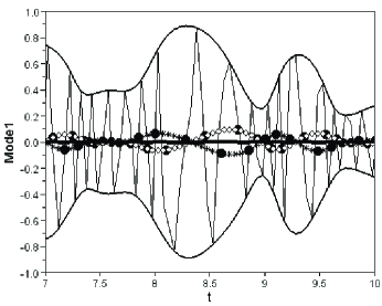
According to the number of interpolating curves, we classify ESMD into ESMD_I, ESMD_II, ESMD_III, $\cdots$. In fact, their differences lie in the request on the equilibrium variation $A_{e}(t)\cos{\theta_{e}(t)}$ which should be understood as an interpolating function with all the midpoints. ESMD_I adopts a rigid extreme-point symmetry in the sifting process which requires all the midpoints almost lying on the zero line, that is, $A_{e}(t)\approx 0$. For this case, all the IMFs should almost degenerate to the equal-amplitude form $A_{r}\cos{\theta_{r}(t)}$. From the viewpoint of physics, this strategy is too rigorous. ESMD_II extends the concept of the extreme-point symmetry, which permits the location shifting of the midpoint in such a manner: The trajectory variation $A_{e}(t)\cos{\theta_{e}(t)}$ should be envelop-symmetric about its odd and even interpolating curves. These two envelops differ from the common positive and negative outer envelops, after all, they may change their signs alternately. The sifting test results show that this odd-even type of extreme-point symmetry for ESMD_II is almost equivalent to the outer envelop symmetry for EMD (see Fig.17). ESMD_III gives a further extension to the concept of extreme-point symmetry. It liberalizes the restriction on $A_{e}(t)\cos{\theta_{e}(t)}$ and only requires the sum of two interpolating curves to be symmetric with the third one. Certainly, the restriction on $A_{e}(t)\cos{\theta_{e}(t)}$ can be also liberalized in this way with more interpolating curves.

1.4 About the Instantaneous Frequency

The definition of the instantaneous frequency is a controversial issue [Huang et al. (2009a)]. As analyzed above, only when a quantity varies in a periodic oscillating manner, the frequency can be understood as an oscillating change rate during the process of moving back and forth. So there is no local meaning for frequency at a given point. But as argued by Huang et al. (2009a) and the references therein, there is indeed a frequency modulating phenomenon. Therefore, to accord with the generalized periodic function $A(t)\cos{\theta(t)}$ in mathematics, the derivative form $\omega(t)=d\theta/{dt}$ is recommended. To be physically meaningful, it requires $d\theta/{dt}\geq 0$. However, for a decomposed IMF with denotation $x(t)$, this calculation is not trivial. In order to solve this problem, Huang et al. suggested the Hilbert transform which is popular used nowadays:

$$y(t)=H[x(t)]=\frac{1}{\pi}P\int_{-\infty}^{\infty}\frac{x(\tau)}{t-\tau}d\tau,$$ (3)

in which $P$ indicates the principal value of the singular integral. With the Hilbert transform, the analytic data is defined as

$$z(t)=x(t)+iy(t)=A(t)e^{i\theta(t)},$$ (4)

where

$$A(t)=\sqrt{x^{2}(t)+y^{2}(t)},\qquad\theta(t)=\arctan\left(\frac{y(t)}{x(t)}\right).$$ (5)

Here $A(t)$ is the instantaneous amplitude and $\theta(t)$ is the phase function. Furthermore, the instantaneous frequency can be calculated by $\omega(t)=d\theta/{dt}$.

Essentially, the Eqn.(3) defines the Hilbert transform as the convolution of $x(t)$ and $1/t$, therefore, it emphasizes the local properties of $x(t)$. In Eqn.(4) the polar coordinate expression further clarifies the local nature of this representation: it is the best local fit of an amplitude and phase varying trigonometric function to $z(t)$ [Huang and Shen (2005)]. In this sense, the Hilbert transform is superior to the Fourier transform, Wavelet transform and other analytical forms. However, this approach has a disadvantage in unsatisfying the quadrature request delimited by the well-known Bedrosian and Nuttall theorems. That is, in order to use Eqn.(4) $y(t)$ should be a quadrature function of $x(t)$. In addition, to get a meaningful instantaneous frequency it also needs a hypothesis that the positive derivative of $\theta(t)$ exists.

In fact, no matter how the integral transform is defined, it is actually a uniform running-mean processing. Now that the processing is done on the data, why not calculate the instantaneous frequency from the data in a direct way? Historically speaking, there are only crude estimation methods for the frequency change. Just as reviewed by Huang et al. (2009a), there is a fundamental “zero-crossing method” which has been used for a long time to compute the mean period (frequency) for narrow band data. Of course, this approach is only meaningful for mono-component functions, where the numbers of zero-crossings and extreme points must be equal in the data. Huang et al. had generalized the zero-crossing method by improving the temporal resolution to a quarter wave period with a running-mean approach. This improvement yields a better estimation for the frequency, but it is still incapable of reflecting the instantaneous changes.

Figure 1: An example of periodic oscillation with intermittences.

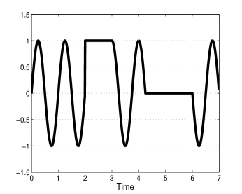
As an instantaneous frequency, it should be capable of reflecting the intermittent case as in Fig.1, rather than excluding the adjacent-equal situation. While the oscillation maintains unchanged at the extrema, the zero-crossing or any other locations its instantaneous frequency should be all $0$. Certainly, the frequency may lose its meaning on the junctures (belong to a null set). It doesn’t matter, after all, the data itself is not smooth. Now that the period should be defined relative to a segment of time and the frequency needs to be understood point by point, we can conciliate this conflict by an interpolating method. With this understanding, we have developed a “direct interpolating” approach for the calculation of the instantaneous frequency which will be illustrated in a latter section.

1.5 About the Definition of IMF

The EMD method defines an intrinsic mode function (IMF) with the following two conditions [Huang et al. (1998), Huang and Shen (2005)]:
(1) In the whole data set, the number of extreme points and the number of zero-crossings must either equal or differ at most by one.
(2) At any point, the mean value of the envelope defined by the local maxima and the envelope defined by the local minima is zero.

The first condition can be understood as: the IMF’s local maxima and minima points are septal with no adjacent zero-crossings, all its maxima should be positive and all its minima should be negative. Just as stated by Huang et al. (1998), this request on oscillating manner is for the rationality of defining an instantaneous frequency. According to this restriction, the function given in Fig.1 is not an IMF. But from the viewpoint of physics, the occurrence of this intermittence phenomenon is possible. Therefore, it is reasonable for liberalizing the restriction and counting it as an IMF.

The second condition requires that an IMF must have an envelope symmetry. This restriction is for convenience of deducing a meaningful instantaneous frequency by means of the Hilbert transform. Now that the Hilbert transform is abandoned and the “direct interpolating” approach is adopted, the restriction should be liberalized. In fact, just as stated in our previous paper [Wang and Li (2012a)] the rigid envelope-symmetric IMFs are out of reach for an actual data processing test. Therefore, only if a decomposed component satisfies a certain error requirement it can be seen as an IMF. In addition, notice that the odd-even type of the extreme-point symmetry for ESMD_II is almost equivalent to the envelop symmetry for EMD and the three-curve type for ESMD_III is more general than the envelop symmetry, this request can be also liberalized.

Based on the above analysis, the definition of IMF can be extended with the following two conditions:
(1) To count all the adjacent equal extreme points as one, the local maxima and minima points should be septal, all its maxima should be positive and all its minima should be negative.
(2) It should be almost envelop-symmetric or extreme-point symmetric in the generalized sense.
We note that the envelop symmetry and the odd-even type of the extreme-point symmetry are very good types which yield IMFs with suitable amplitude and frequency modulations, and too low request on symmetry would lead to difficulty to frequency and energy analysis.

2 Decomposition Algorithm for ESMD Method

We begin to introduce the ESMD method with the decomposition algorithm. In the present paper, only one-dimensional data are considered. Certainly, there is a precondition for the processing that the sampling rate of the observational instruments should be known. It is a common sense that the local maxima and minima points are septal with counting all the adjacent equal extreme points as one. For convenience of programming, in case there are several adjacent equal extreme points, we only choose the first one as a representative. The program code is exploited on the Scilab platform and the algorithm is as follows:

Step 1: Find all the local extreme points (maxima points plus minima points) of the data $Y$ and numerate them by $E_{i}$ with $1\leq i\leq n$.

Step 2: Connect all the adjacent $E_{i}$ with line segments and mark their midpoints by $F_{i}$ with $1\leq i\leq n-1$.

Step 3: Add a left and a right boundary midpoints $F_{0}$ and $F_{n}$ through a certain approach.

Step 4: Construct $p$ interpolating curves $L_{1},\cdots,L_{p}$ ($p\geq 1$) with all these $n+1$ midpoints and calculate their mean value by $L^{*}=(L_{1}+\cdots+L_{p})/p$.

Step 5: Repeat the above four steps on $Y-L^{*}$ until $|L^{*}|\leq\varepsilon$ ($\varepsilon$ is a permitted error) or the sifting times attain a preset maximum number $K$. At this time, we get the first mode $M_{1}$.

Step 6: Repeat the above five steps on the residual $Y-M_{1}$ and get $M_{2},M_{3}\cdots$ until the last residual $R$ with no more than a certain number of extreme points.

Step 7: Change the maximum number $K$ on a finite integer interval $[K_{min},K_{max}]$ and repeat the above six steps. Then calculate the variance $\sigma^{2}$ of $Y-R$ and plot a figure with $\sigma/\sigma_{0}$ and $K$, here $\sigma_{0}$ is the standard deviation of $Y$.

Step 8: Find the number $K_{0}$ which accords with minimum $\sigma/\sigma_{0}$ on $[K_{min},K_{max}]$. Then use this $K_{0}$ to repeat the previous six steps and output the whole modes. At this time, the last residual $R$ is actually an optimal AGM curve.

There are several questions associated with this algorithm. In the following we explain them one by one.

According to the fourth step, we classify the ESMD into ESMD_I, ESMD_II, ESMD_III, $\cdots$. ESMD_I does the sifting process by using only $1$ curve interpolated by all the midpoints; ESMD_II does the sifting process by using $2$ curves interpolated by the odd and even midpoints, respectively; ESMD_III does the sifting process by using $3$ curves interpolated by the midpoints numerated by $3k+1$, $3k+2$ and $3(k+1)$ ($k=0,1,\cdots$), respectively. Certainly, we can also define other schemes with more interpolating curves according to this method.

In the fifth step, besides the permitted error $\varepsilon$, we can also adjust the maximum sifting times $K$. On the one hand, if $\varepsilon$ is the unique controlling parameter, it may leads to an endless loop to the decomposition; On the other hand, if $K$ is the unique controlling parameter, we know nothing about the symmetric properties of each mode. Perhaps a small number of sifting may lead to good symmetric to a mode. So the wise choice is to use them all. To obtain a series of relatively reliable modes, we can fix $\varepsilon$ to be a very small value and control the decomposing process by changing $K$ on a finite integer interval such that the last residual $R$ (AGM curve) is an optimal one. So Step $7$ and $8$ are very necessary. In fact, only when the fitting curve of the data is an optimal one, the remainder can be seen as an actual oscillation caused by a series of wave fluctuations.

Denote the original data and the AGM curve by $Y=\{y_{i}\}_{i=1}^{N}$ and $R=\{r_{i}\}_{i=1}^{N}$, respectively. Commonly, relative to its total mean $\overline{Y}=\sum_{i=1}^{N}y_{i}/N$ the variance of the data is defined as

$$\sigma_{0}^{2}=\frac{1}{N}\sum\limits_{i=1}^{N}(y_{i}-\overline{Y})^{2}.$$ (6)

Here we define the variance relative to the AGM by

$$\sigma^{2}=\frac{1}{N}\sum\limits_{i=1}^{N}(y_{i}-r_{i})^{2}.$$ (7)

In the applications, we usually choose $\varepsilon=0.001\sigma_{0}$ and use the ratio $\nu=\sigma/\sigma_{0}$ to reflect the degree of optimization for the AGM relative to the common total mean.

In addition, the third step is associated with a boundary processing which is a “benevolent see benevolence” problem. In our program codes we have developed the linear interpolation method given by Wu and Huang (2009) and revised the interpolation styles for the too steep boundary case [see Appendix A]. This revision can make the boundary much more stable, even for the tests with $100,000$ sifting times [Wang and Li (2012a)]. In the following we test the decomposition effectiveness according to ESMD_I, ESMD_II and ESMD_III and our attention is mainly focused on the second one.

3 Performance of ESMD_I

ESMD_I does the sifting process by using only $1$ curve interpolated by all the midpoints of the line segments between the local maxima and minima points. Though this case has been discussed by Huang et al.(1998), it is worth reemphasizing from the viewpoint of ESMD. We test it by a simple example as follows. Example 1: $Y(t)=e^{-0.1t}\sin{(\pi t/2+\pi/3)}$ with $0\leq t\leq 20$. This is a weighted-periodic function with a fixed frequency and varying amplitude. A data may maintain its oscillating frequency and increase (or decrease) its amplitude with gaining (or losing) energy. So it is a very natural thing to meet the weighted-periodic function in data processing. A good sifting scheme is anticipated yielding a unique IMF with a small decomposition error.

Figure 2: All the midpoints (circle points) of the line segments between the local maxima and minima points and their unique interpolating curve (bulk inner curve).

Figure 3: The decomposition result for the weighted-periodic function given by ESMD_I with 20 sifting times, here the horizontal axis stands for the time (second).

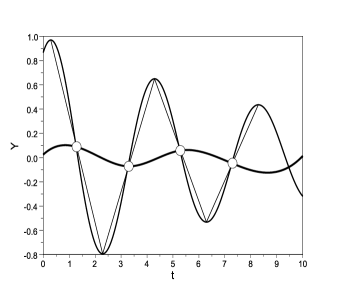
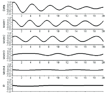
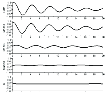
The detailed constructing process of the interpolating curve is shown in Fig.2. If there is no variance-ratio investigations, we know nothing about the effect of sifting times. To try the decomposition with $20$ times sifting, it yields a result in Fig.3, which includes $4$ modes and a residual R. There is a common feature for these modes that all their amplitudes almost maintain unchanged. In fact, it is due to the scheme of the rigid extreme-point symmetry adopted by ESMD_I. Through a simple geometric proof we see a curve with an equal amplitude in the form $A\sin{\theta(t)}$ ($\theta(t)$ is an increasing function) must be an extreme-point symmetric one. Vice versa, it is also true. Particularly, the Mode1 is not only extreme-point symmetric but also periodic. In fact, it is an approximation of the function $0.6\sin{(\pi t/2+\pi/3)}$ which carries the most periodicity of the original data. This try shows that $20$ times sifting accords with an enough-symmetry and slow-efficiency case. Hence, a lower times with lose symmetry request may be better. but there is no effective criteria for it under the EMD circumstance. One progress of ESMD is on the adoption of variance ratio.

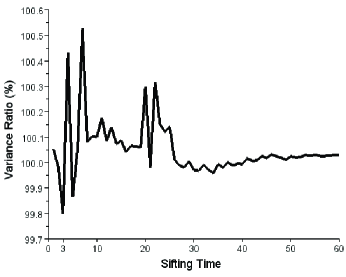
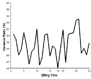
Firstly, we plot the distribution figure of the variance ratio $\nu=\sigma/\sigma_{0}$ along the sifting times (see Fig.4) and find out the optimal sifting time $3$ which accords with the minimum value $\nu=99.8\%$; Secondly, we output the corresponding decomposition result with $3$ sifting times. It follows from Fig.5 that the result is better than that in Fig.3 with $20$ times sifting, where Mode1 can be seen as an approximation of the original data and the others can be seen as the decomposition error. Certainly, this decomposition is not perfect either, after all, the error amplitude achieves $0.3$.

Figure 4: The distribution of variance ratio $\nu=\sigma/\sigma_{0}$ along the sifting times for the weighted-periodic function.

Figure 5: The decomposition result for the weighted-periodic function given by ESMD_I with $3$ sifting times, here the horizontal axis stands for the time (second).

Example 2: A segment of wind data observed at sea with $20$Hz sampling rate.

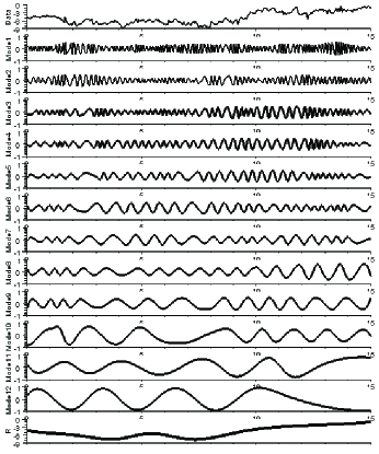
It follows from Fig.6 that $18$ is the optimal sifting times in the interval $[1,30]$. The corresponding decomposition in Fig.7 yields $12$ IMFs together with a residual R with $40\%$ variance ratio. It means the AGM is the best fitting curve of the wind data. At this time, the IMFs still have an amplitude-modulation phenomenon. If the sifting times is added, more and more equal-amplitude IMFs may appear. In consideration of physical meaning stated by Huang et al. (2003), we do not expect too many equal-amplitude modes. So the lower sifting times with imperfect decomposition is preferred for ESMD_I.

Figure 6: The distribution of variance ratio $\nu=\sigma/\sigma_{0}$ along the sifting times for the wind data.

Figure 7: The decomposition result for the wind data given by ESMD_I with $18$ sifting times, here the horizontal axis stands for the time (second).

In all, due to the adoption of a scheme with the rigid extreme-point symmetry, the decomposition efficiency of ESMD_I is not high. Besides the rigorous request of symmetry, there is also another aspect. It follows from Fig.2 that when all of the midpoints are used for interpolating, the generated curve may contain almost the same number of extreme points as the original data which may subsequently enter into the second mode. This also leads to low efficiency to the decomposition. Though ESMD_I has this defect, its AGM curve may be very good. Comparatively, the EMD method has a relatively high decomposing efficiency. One reason is that, the request of envelope symmetry is lower than that of the rigid extreme-point symmetry; Another reason is that, the upper and lower envelopes are interpolated by almost half number of the data’s extreme points and their mean curve discounts the number by almost a half. In view of these facts, it is very natural to do the decomposition by using $2$ interpolating curves.

4 Performance of ESMD_II

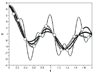
ESMD_II does the sifting process by using $2$ curves interpolated by the odd and even midpoints, respectively. The detailed constructing process of the curves is shown in Fig.8. For this case, the decomposition of Example 1 is trivial since the original curve itself is a permitted mode. In the following we test ESMD_II by three examples and analyze its characteristics in three aspects.

Figure 8: All the midpoints (big circle points) of the line segments between the local maxima and minima points of the data (thin solid curve) and the mean curve (thick solid curve) of their odd and even interpolating curves.

4.1 Decomposition Tests

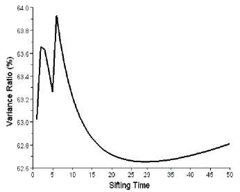
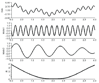
Example 3: $Y(t)=-\sin(8\pi t)+1.5e^{-0.2t}\sin{(1.9\pi t+\pi/20)}+(t-2)^{2}$, $0\leq t\leq 4$. This data is composed of one periodic function, one weighted-periodic function and one parabola. In the following we do the decomposition with ESMD_II. From Fig.9 and 10 we see the decomposition is perfect. Mode1 accords with the periodic function; Mode2 accords with the weighted-periodic function; The residual R accords with the parabola.

Figure 9: The distribution of variance ratio $\nu=\sigma/\sigma_{0}$ along the sifting times for the composed data.

Figure 10: The decomposition result for the composed data given by ESMD_II with $29$ sifting times, here the horizontal axis stands for the time (second).

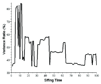
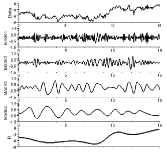
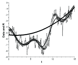
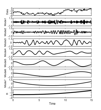
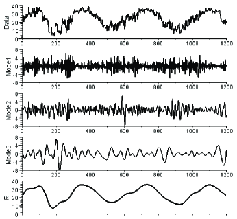
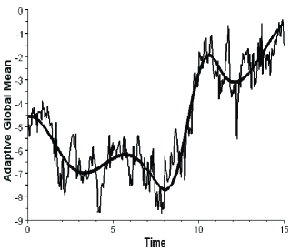
In the following we re-decompose Example 2 with ESMD_II. From Fig.11 we see the variance ratio $\nu=\sigma/\sigma_{0}$ attains its minimum value at $30$, which can be seen as an optimal sifting times in the whole interval $[1,100]$. Fig.12 shows the corresponding decomposition which is more distinct than that in Fig.7 given by ESMD_I. The decomposed IMFs accord with the components of the wind turbulence with average periods $3.8$s, $1.5$s, $0.6$s,$\cdots$. In addition, the last residual R is an optimal AGM curve, which reflects the fundamental evolutionary trend of the wind speed very well (see Fig.13). Certainly, there is a necessity for us to compare with EMD method. So the test is also done on the code eemd.m (downloaded from http://rcada.ncu.edu.tw/class2009.htm) for the non-noise case. By the way, to be more objective, the default $10$ times sifting given by Wu and Huang (2009) is substituted by $30$ here. From Fig.12 and Fig.14 we see the difference is very clear. This difference probably lies in the sifting scheme, the boundary processing and the programming. Certainly, it is difficult for us to judge which IMF set is more reasonable. But it follows from the residual comparison in Fig.13 we see the global mean curve given by ESMD_II is better than the monotone form given by the EMD method, after all, this one is found by an optimizing approach. It also indicates that the AGM curve is almost equivalent to the sum of Mode5, Mode6, Mode7 and the last trend function of EMD. Generally speaking, the global mean curve is a component with maximum magnitude, its deviation would lead to large distortion to the oscillating IMFs. So in this sense, ESMD_II is preferable.

Figure 11: The distribution of the variance ratio $\nu=\sigma/\sigma_{0}$ along the sifting times for the wind data.

Figure 12: The decomposition result for the wind data given by ESMD_II with $30$ sifting times, here the horizontal axis stands for the time (second).

Figure 13: Comparison between the AGM curve of ESMD_II (the curve with small circles), the trend function (thick solid curve) as well as the sum of R and Mode5-7 of EMD (thin solid curve), where the dotted curve stands for the wind data.

Figure 14: The decomposition result for the wind data given by EMD method with $30$ sifting times.

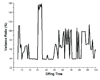
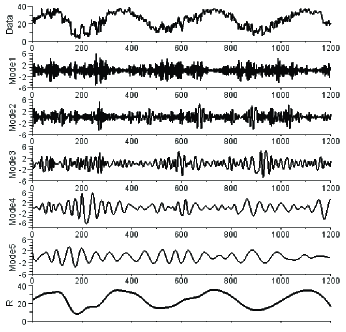
Example 4: The day-averaged air temperature data from May 10, 2008 to Nov. 3, 2011 downloaded from the National Climatic Data Center of America. From Fig.15 we see the variance ratio has some septal stable intervals, such as $[20,29]$, $[36,40]$, $[43,48]$ and $[72,76]$. On all these stable intervals, the variance ratio is almost identical, which leads to almost the same result to the decomposition. At this time the optimal sifting time is $29$, even when the whole interval is prolonged to $[1,200]$. The decomposition in Fig.16 shows a very good seasonal evolutionary trend for the air temperature. The decomposed IMFs accord with the components with average periods $66$ day, $35$ day, $17$ day,$\cdots$, which can be understood as bimonthly, monthly, semimonthly,$\cdots$ temperature oscillations. We refer the readers to Huang et al. (2009b) and Bao et al. (2011) for the analyzing approach. Particularly, we can judge the period and time of the temperature anomaly from the amplitude variation. For this case, the amplitude variation of Mode5 is small, yet that of Mode4 is very big. These indicate that the temperature anomaly mainly occurs on time-scale of 35 days in Jan.-Mar., 2009.

Figure 15: The distribution of variance ratio $\nu=\sigma/\sigma_{0}$ along the sifting times for the temperature data.

Figure 16: The decomposition result for the temperature data given by ESMD_II with $29$ sifting times, here the horizontal axis stands for the time (day).

4.2 Symmetry Characteristic of the Modes

When the decomposed mode is a periodic function, such as Mode1 in Fig.10, its symmetry characteristic is very obvious. For this case, bother the odd and even interpolating curves and their mean value all approximate the zero line. This is a real extreme-point symmetry. But if the decomposed mode is a weighted-periodic function, such as Mode2 in Fig.10, its symmetry is an extreme-point symmetry of odd-even type, which only requires the symmetry between the odd and even interpolating curves. In fact, this phenomenon is very universal. For an actual data component, not only its amplitude but also its frequency changes along the time, such as Mode1 in Fig.12. It follows from Fig.17 that this case is almost equivalent to the envelope symmetry. However, since the magnitudes of the odd and even interpolating curves are smaller than that of the upper and lower envelopes, the convergence speed of their mean curve to the zero line may be quicker. So the ESMD_II method may need less sifting times than that of the EMD method to reach a relatively stable state.

4.3 Effect of Sifting Times to the Decomposition

According to the ESMD algorithm Step 4 and 5, adding the sifting times may make the modes more and more symmetric until $|L^{*}|\leq\varepsilon$. Moreover, since the permitted error $\varepsilon$ is preestablished (such as $\varepsilon=0.001\sigma_{0}$), more times of sifting may imply more symmetric modes. So we can anticipate a finite times of sifting such that all the modes satisfy this permitted error. This case accords with a relatively stable variance ratio $\nu=\sigma/\sigma_{0}$. For Fig.9 the stable interval is approximately $[25,34]$; For Fig.11 and Fig.15 there are several septal stable intervals. In the symmetry requirement we prefer to choose the optimal sifting times in the stable intervals, though there may be some lower sifting times which accord with lower $\nu$. By the way, it is not the case that more times of sifting leads to a better decomposition. On the one hand, as shown in Fig.9, the additional sifting may lead to additional error to the decomposition; On the other hand, as shown in Fig.15, the decomposition may be not uniform convergent about the sifting times. Certainly, there is also another case that the stable interval does not appear for several hundred times of sifting. This is possibly caused by a too small value of $\varepsilon$. At this time, we suggest replacing the value of $\varepsilon$ by a bigger one and redoing it. In addition, we note that in the stable interval the decomposition is insensitive to the sifting times and, on the contrary, in the unstable interval it differs much. Especially, when the variance ratio $\nu>100\%$, the corresponding decomposition may be very bad.

4.4 Effect of Least Extreme-Point Number to the Decomposition

To stop the decomposition it requires the least number of extreme points. This number, denoted by $m_{R}$, may influence the shape of R. In order to satisfy the requirement of the linear interpolation on the boundaries, it requires $m_{R}\geq 4$. The default one is $4$. If the so-called optimal R for the default case has large difference from the data (reflected by a very high $\nu$), we can increase $m_{R}$ and redo it to get a better one. Fig.9 and 10 are the default decompositions; Fig.11 and 12 are the decompositions with $m_{R}=6$; Fig.15 and 16 are the decompositions with $m_{R}=8$. In Fig.16 if $m_{R}$ is increased to $20$ the AGM curve may become the combination of Mode5 and R which should be avoided, though the variance ratio is much lowered down at this time.

Figure 17: The odd-even type of extreme-point symmetry for Mode$1$ of Fig.12 (symmetry between the inner curves with $\ast$ and $\diamond$). Here two outer envelop curves are also shown.

Figure 18: The decomposition result for the temperature data given by ESMD_III with $11$ sifting times, here the horizontal axis stands for the time (day).

5 Performance of ESMD_III

ESMD_III does the sifting process by using $3$ curves $L_{1},L_{2}$ and $L_{3}$ interpolated by the midpoints numerated by $3k+1$, $3k+2$ and $3(k+1)$ ($k=0,1,\cdots$), respectively. For this case the mean curve is defined as $L^{*}=(L_{1}+L_{2}+L_{3})/3$. To make a mode symmetric it requires $|L^{*}|\leq\varepsilon$. This kind of symmetry is an extreme-point symmetry in the more extensive meaning, which only requires the symmetry between $L_{1}+L_{2}$ and $L_{3}$. Particularly, if the component is a periodic function it becomes a real extreme-point symmetry; if the component is a weighted-periodic function it degenerates to the odd-even type of extreme-point symmetry. So ESMD_III can give almost the same decomposition result as ESMD_II for Example 3. By the way, for this case ESMD_III only needs $5$ sifting times, which is much less than $29$ for ESMD_II.

It follows from Fig.18 that ESMD_III also outputs good AGM curve for the temperature data. Its $11$ times sifting yields a variance ratio $36.97\%$, which is slightly smaller than $37.11\%$ obtained by ESMD_II with $29$ times sifting. By making comparison with Fig.16, we see ESMD_III yields less modes than that of ESMD_II. One reason is that, relative to the odd-even interpolation, the $3$-curve one gives much quicker decreasing to the number of extreme points; Another reason is that, ESMD_III adopts a lower type of symmetry.

6 Direct Interpolating Approach for Instantaneous Frequency and Amplitude

Now that the period should be defined relative to a segment of time and the frequency needs to be understood point by point, we conciliate this conflict by developing a “direct interpolating (DI)” approach for it. Just as analyzed in Section 1.4, the instantaneous frequency should be capable of reflecting the intermittent case in Fig.1, rather than excluding the adjacent-equal situation. The detailed interpolation algorithm is as follows.

6.1 Interpolation Algorithm

For the decomposed $n$ IMFs we calculate their instantaneous frequencies by implementing the following algorithm:

Step 1: For each IMF (denoted by $(t(k),y(k))$ with $1\leq k\leq N$) find all the interpolating points which satisfy: $y(k)>y(k-1)\;\&\;y(k)\geq y(k+1)$, $y(k)\geq y(k-1)\;\&\;y(k)>y(k+1)$, $y(k)<y(k-1)\;\&\;y(k)\leq y(k+1)$ or $y(k)\leq y(k-1)\;\&\;y(k)<y(k+1)$ and numerate them by $E_{i}(t_{i},y_{i})$ with $1\leq i\leq m$.

Step 2: If there are two adjacent $E_{i}$ such that $y_{i-1}=y_{i}$ or $y_{i}=y_{i+1}$, then define the frequency interpolation coordinates by $a_{i}=t(i),f_{i}=0$; further if $E_{i}$ and $E_{i+1}$ are adjacent extreme points, then define $a_{i-1}=(t_{i}+t_{i-2})/2,f_{i-1}=1/(t_{i}-t_{i-2})$ and $a_{i+2}=(t_{i+3}+t_{i+1})/2,f_{i+2}=1/(t_{i+3}-t_{i+1})$; else if $E_{i}$ and $E_{i+1}$ (or $E_{i-1}$ and $E_{i}$) are not adjacent extreme points, then define $a_{i-1}=t_{i-1},f_{i-1}=1/[(t_{i+2}-t_{i-2})-(t_{i+1}-t_{i})]$ and $a_{i+2}=t_{i+2},f_{i+2}=1/[(t_{i+3}-t_{i-1})-(t_{i+1}-t_{i})]$; else, define $a_{i}=(t_{i+1}+t_{i-1})/2,f_{i}=1/(t_{i+1}-t_{i-1})$.

Step 3: To add the boundary points with a linear interpolating method. For the left one, if it is an adjacent equal case, assign the value $f_{1}=0$ to $a_{1}=t(1)$; if not, assign the value $f_{1}=(f_{3}-f_{2})(a_{1}-a_{2})/(a_{3}-a_{2})+f_{2}$ to $a_{1}=t(1)$; further if $f_{1}\leq 0$ then assign $f_{1}=1/[2(t_{2}-t_{1})]$ to $a_{1}=t(1)$. For the right one, if it is an adjacent equal case, assign the value $f_{m}=0$ to $a_{m}=t(N)$; if not, assign the value $f_{m}=(f_{m-1}-f_{m-2})(a_{m}-a_{m-1})/(a_{m-1}-a_{m-2})+f_{m-1}$ to $a_{m}=t(N)$; further if $f_{m}\leq 0$ then assign $f_{m}=1/[2(t_{m}-t_{m-1})]$ to $a_{m}=t(N)$.

Step 4: To make the interpolation with all the discrete points $(a_{i},f_{i})$ and get a curve $f(t)$. To be meaningful, we define the instantaneous frequency curve by $\max\{0,\;f(t)\}$.

Step 5: To output subplot frequency figures for all IMFs.

In addition, since the interpolating method for the instantaneous amplitude is much simpler, we omit its algorithm. For an IMF, its instantaneous amplitude curve can be understood as the upper envelop interpolated by all the maxima points of this IMF in the absolute-value form (rely on all the extreme points of the original one). In fact, for an IMF obtained under the envelop-symmetry scheme or the odd-even extreme-point symmetry scheme, its amplitude curve is almost equivalent to the upper envelop of the IMF itself with the slow modulation. But for the three-curve type the amplitude may have too quick modulation which is not preferred. By the way, to reflect the energy variation in a distinct way, the instantaneous amplitude and frequency can be figured out together.

6.2 Performance of DI Approach

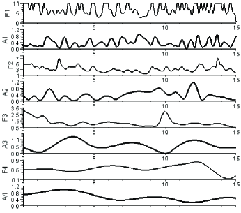
In the following we test the DI approach with the decomposition results given in Fig.12. By executing the previous algorithm on the $4$ IMFs it yields instantaneous frequencies and amplitudes in Fig.19. It follows from F1 that there are several segments on which the instantaneous frequency attains the Nyquist frequency $f_{N}=f/2$, here $f=20$Hz stands for the sampling rate of the wind data. For a given IMF, such as the third one, this kind of figure can reflect clear variation of the frequency and amplitude. The comparison between F3 and A3 shows that, at $t=10$s, the third IMF has a sharp oscillation with a very small amplitude.

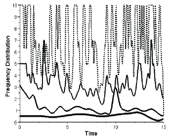
Besides reflecting the time-variation of amplitude and frequency, the DI approach can also provide an intuitional frequency distribution for the IMFs (see Fig.20). It gives us a new understanding on the decomposition. Though, the neighboring two modes may have the same frequency on the whole, this state rarely occurs at the same time. In another word, the frequencies of these two neighboring modes do not overlap at the same time for almost all the case. So the so-called “frequency-overlapping puzzle” is not a real puzzle in the sense of time-variation. With this understanding, the decomposed modes can be seen as independent ones. Each one represents an individual component which accords with a specific physical oscillation. Certainly, it needs a mathematical theory to support the decomposition methodology. It is the second attractive topic of this paper left for mathematicians.

Figure 19: The instantaneous frequency (F) and amplitude (A) variations of the IMFs for the wind data along the time.

Figure 20: The frequency distribution of the IMFs for the wind data.

Since the frequency and amplitude (energy) of each IMF shift at any time, it is unreasonable to project the total energy onto a series of frequencies as a Fourier frequency-spectrum or a Hilbert time-frequency-spectrum, after all, the total energy itself changes along the time. With this understanding we abandon the spectrum method and turn to discussing the time-variation of the total energy. According to the state in Section 1.3, the $j$-th IMF almost accord with the mathematical expression $x_{j}(t)=A_{j}(t)\cos{\theta_{j}(t)}$ ($1\leq j\leq n$), here $A_{j}(t)$ is actually the called amplitude curve. Taking ESMD_II as a default decomposition, the odd-even extreme-point symmetry scheme assigns $A_{j}(t)$ a slow modulation feather. Based on this consideration, we define the so-called total energy in the form of kinetic energy:

$$E(t)=\frac{1}{2}\sum\limits_{j=1}^{n}A^{2}_{j}(t).$$ (8)

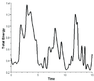
Certainly, here the word “total energy” is in a general sense. For the temperature data, it can be understood as the whole oscillation intensity of the temperature. By using this definition, we get the corresponding variation of the total energy for the wind data. It follows from Fig.21 that the total energy of IMFs has three large peaks in the $15$s time segment. By making comparison with Fig.22 we see these peaks accord just right with the sunk parts of the AGM. This is a very interesting phenomenon. Perhaps it is caused by the energy transfer; perhaps it is just a coincidence; perhaps there are other deep causes. It is the third attractive topic of this paper left for further discussion.

Figure 21: The time-variation of the total energy for all the IMFs of the wind data.

Figure 22: The variation of the optimal AGM curve for the wind data along the time.

7 Summary

In order to analyze the non-stationary data, an “extreme-point symmetric mode decomposition (ESMD)” method is proposed. There are two parts for it: the first part is the decomposition approach which yields a series of intrinsic mode functions (IMFs) together with an optimal “adaptive global mean (AGM)” curve, the second part is the “direct interpolating (DI)” approach which yields instantaneous amplitudes and frequencies for the IMFs together with a time-varying total energy. It can be seen as an alternate of the well-known “Hilbert-Huang transform (HHT)” method with the following five characteristics:
(1) Differing from constructing $2$ outer envelopes, its sifting process is implemented by the aid of $1$, $2$, $3$ or more inner curves interpolated by the midpoints of the line segments connecting the local maxima and minima points. Accordingly, ESMD is classified into ESMD_I, ESMD_II, ESMD_III, etc.
(2) It does not decompose the data to the last trend curve with at most one extreme point, it optimizes the residual component to be an optimal AGM curve which possesses a certain number of extreme points. By the optimizing process one can determine the sifting times and output the optimal decomposition.
(3) The concept of extreme-point symmetry is wider than the envelop symmetry. From the viewpoint of material movement, as a matter of fact, the oscillation occurs around the equilibrium which may also shift during this process. So the extreme-point symmetry actually reflects the local symmetry about itself. ESMD_I adopts a rigid extreme-point symmetry which is more rigorous than envelop symmetry; ESMD_II adopts an odd-even type of extreme-point symmetry which is almost equivalent to the envelop symmetry; ESMD_III adopts a three-curve type of extreme-point symmetry which is more general than the envelop symmetry.
(4) The definition of IMF is extended. The new form not only includes the intermittent case but also looses the requirement on symmetry.
(5) The Hilbert-spectral-analysis approach for instantaneous frequency and amplitude is substituted by the data-based one. This new approach easily conciliates the conflict: the period should be defined relative to a segment of time and the frequency needs to be understood point by point. It is unreasonable to project the total energy onto a series of fixed frequencies as a Fourier frequency-spectrum or a Hilbert time-frequency-spectrum because the total energy itself changes along the time. The DI approach can not only yield clear distribution for instantaneous frequency and amplitude but also reflect the time-variation of total energy in a distinct way.

Comparing ESMD_I, ESMD_II and ESMD_III reveals that, as the number of interpolating curves increases, 1) the mode number decreases; 2) the symmetry degree decreases; 3) the amplitude modulation increases; 4) the decomposition efficiency increases (needs less sifting times). With these understandings, we prefer doing the decomposition with the eclectic one. In fact, ESMD_I can only yield acceptable imperfect decomposition with low times sifting. The equal-amplitude phenomenon will occur at high sifting times. In order to keep physical meaning this case should be avoided. ESMD_III has high decomposition efficiency, but its low degree of symmetry and quick modulation of amplitude are disadvantageous for frequency and energy analysis. The data processing tests also indicate that ESMD_II is superior to ESMD_I and ESMD_III and its decomposition result is more preferable. In addition, from the first try on ESMD_I to the successful exploitations of ESMD_II and ESMD_III it costs us two years time. Besides this paper, we have also developed a software which is now protected by the National Copyright Administration of China [Wang and Li (2012), Wang and Li (2012b)]. ESMD_II is anticipated an effective usage in the fields of atmospheric and oceanic sciences, informatics, economics, ecology, medicine and seismology, etc.

Though these three types of interpolation have much difference, they have a mutual advantage. All of them can output good AGM curve. In fact, this advantage owes to the inner interpolation. Besides the decomposition, the ESMD method also offers a good adaptive approach for data fitting. It is superior to the common least-square method and running mean approach. In fact, the first one is awkward in application due to the request on a priori function form, the second one lacks of theoretical basis and different choices of time windows and weight coefficients may result in different curves.

We note that the type of interpolation is not essential, the approach developed here is also suitable for the envelop-symmetric scheme adopted by the EMD method [see Appendix B]. As the stoppage criterion concerned, our strategy is an synthetic one. A preset-error condition is adopted to ensure the symmetry and an ensemble optimal-sifting-times (OST) scheme is chosen to optimize the whole decomposition. In addition to this stoppage criterion there is also another applicable one. In fact, in view of the intermittent feature of IMF’s symmetry [Wang and Li (2012a)], we can abandon the preset-error condition and execute the OST processing repeatedly and draw out a series of IMFs. If the mode symmetry is merely concerned this approach is a better choice, but it follows from the test in Appendix C that the last residual may be an inferior one. In order to make up this defect, one can further implement the ensemble OST scheme on the whole IMF sets. Certainly, its time-consuming would be longer than the present one. The last appendix is about the asymptotic behavior of the modes along sifting times.

Acknowledgments. Firstly, we thank Professor Norden E. Huang for his enthusiastic encouragement and many stimulating discussions on the topics related to the present research; Secondly, we thank Professor Xian-Yao Chen for his help in the manuscript revision; Thirdly, we thank the support from the Shandong Province Natural Science Fund, P.R. China (No.ZR2012DM004).

Appendix A: Boundary Processing

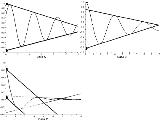
In our program codes we have developed the linear interpolation method given by Wu and Huang (2009) and revised the interpolation styles for the too steep boundary case. This revision can make the boundary much more stable, even for the tests given by Wang and Li (2012a) with $100,000$ sifting times. Take the left boundary processing as an example. Let $y(t)=k_{1}t+b_{1}$ and $y(t)=k_{2}t+b_{2}$ be the upper and lower lines interpolated by the first two maxima and minima points, respectively. Also denote the first point of the data by $Y_{1}$. According to Wu and Huang’s classification, (1) if $b_{2}\leq Y_{1}\leq b_{1}$, then define $b_{1}$ and $b_{2}$ as the boundary maximum and minimum points, respectively; (2) if $Y_{1}>b_{1}$ (or $Y_{1}<b_{2}$), then define $Y_{1}$ and $b_{2}$ (or $b_{1}$ and $Y_{1}$) as the boundary maximum and minimum points. But if the boundary is too steep (relative to these two interpolating lines), this kind of processing may lead to instability to the decomposition. So we substitute the second term by: (2) if $b_{1}<Y_{1}\leq(b_{1}+b_{2})/2+(b_{1}-b_{2})=(3b_{1}-b_{2})/2$ (or $(3b_{2}-b_{1})/2=(b_{1}+b_{2})/2-(b_{1}-b_{2})\leq Y_{1}<b_{2}$), then define $Y_{1}$ and $b_{2}$ (or $b_{1}$ and $Y_{1}$) as the boundary maximum and minimum points; (3) if $Y_{1}>(3b_{1}-b_{2})/2$ (or $Y_{1}<(3b_{2}-b_{1})/2$), then define $Y_{1}$ as the boundary maximum (minimum) point and take the boundary minimum (maximum) point by using new interpolating line from the first minimum (maximum) point: $y(t)=k^{*}t+b^{*}$, here $k^{*}$ relies on the point $(0,Y_{1})$ and the first maximum (minimum) point. The detailed processing is depicted in Fig.23.

Figure 23: The developed linear interpolation method for the left boundary processing. Case A: $b_{2}\leq Y_{1}\leq b_{1}$; Case B: $b_{1}<Y_{1}\leq(3b_{1}-b_{2})/2$; Case C: $Y_{1}>(3b_{1}-b_{2})/2$.

Appendix B: Decomposition with Envelop-Symmetric Scheme

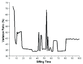
The approach developed in this paper is also suitable for the envelop-symmetric scheme adopted by the EMD method. At this time, the decomposition result is similar to that of odd-even extreme-point symmetric one. To make comparison with ESMD_II at $30$ sifting times, we choose the second optimal one $39$ in the interval $[1,100]$ (the first optimal one is $62$). For this case the AGM curve is as good as ESMD_II with variance ratio $\nu=33.8\%$ and Mode1 and Mode2 are very similar to that of Fig.12. The difference lies in the low-frequency modes (Mode3 and Mode4). This indicates the whole outer symmetry is similar to the local inner symmetry for the case with dense extreme points. But for the sparse case, the outer and inner interpolations may result in different results. Notice that the magnitudes of the upper and lower outer envelopes are bigger than that of odd and even inner curves, their interpolating uncertainty should be bigger than the inner ones for the sparse case. Hence, the result given by ESMD_II should be more credible.

Figure 24: Under the envelop-symmetric scheme, the distribution of the variance ratio $\nu=\sigma/\sigma_{0}$ along the sifting times for the wind data.

Figure 25: Under the envelop-symmetric scheme, the decomposition result for the wind data with $39$ sifting times, here the horizontal axis stands for the time (second).

Appendix C: Decomposition with Optimal-Sifting-Times Approach

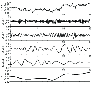
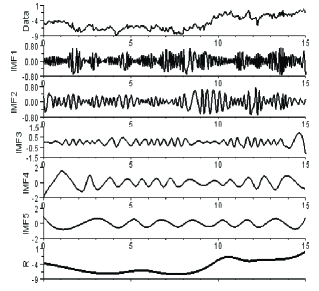
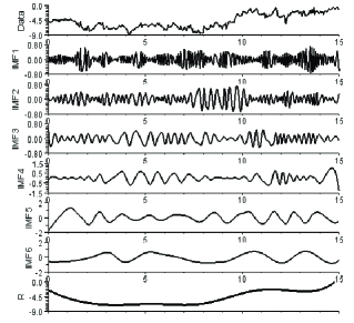
In the following we try another stoppage criterion which is associated with the single usage of optimal-sifting-times (OST) approach. For a preset maximum sifting times $K_{max}$, we can select an optimal one in the integer interval $[1,K_{max}]$ which accords with the minimum value of $A_{max}$, where $A_{max}$ stands for the maximum amplitude of an quasi-mode’s mean cure $L^{*}$. By implementing this OST approach repeatedly we can draw out a series of IMFs. For convenience of processing we take the envelop-symmetric scheme as an example. At this time, $L^{*}$ is simply the mean of the upper and lower envelops and the corresponding decomposition results are given in Fig.26 and 27 with $K_{max}=100$ and $200$, respectively. Though in the interval $[1,200]$ we have more choices and the symmetry of IMFs should be better, its last residual R is worse than that in $[1,100]$. That is to say, the optimal processing on IMFs can not ensure an optimal global mean cure. This defect can be made up by further optimizing $K_{max}$ with respect to the variance ratio $\nu=\sigma/\sigma_{0}$. Certainly, it would cost a longer time-consuming than the one adopted by this paper due to more times of calculation.

Figure 26: Under the envelop-symmetric scheme, the decomposition result for the wind data given by optimal-sifting-times (OST) approach with $K_{{max}}=100$, here the horizontal axis stands for the time (second).

Figure 27: Under the envelop-symmetric scheme, the decomposition result for the wind data given by optimal-sifting-times (OST) approach with $K_{{max}}=200$, here the horizontal axis stands for the time (second).

Appendix D: Asymptotic Behavior of the Modes

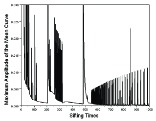
We note that the degree of symmetry does not increase uniformly along the sifting times. Just as indicated by Wang and Li (2012a), its variation behaves in an intermittent manner [see Fig.28]. In addition to it, there is another phenomenon that, by and large, the number of extreme-points for the first mode increases with the sifting times. The ultimate case for it is that all the extreme-points are adjacent with no middle points. At this time, the instantaneous frequency attains its maximum value (equals to the Nyquist frequency). Hence, in order to revealing the intrinsic oscillation of a process through mode decomposition, too high times sifting is not recommended. From our experiential understanding, dozens of times sifting is enough for the ESMD decomposition.

Figure 28: The variation of maximum amplitude for the mean curve of IMF1 along the sifting times, here the wind data is used.

References

- [1] Bao, S. et al. (2011) An empirical study of tropical cyclone activity in the Atlantic and Pacific oceans:1851-2005. Adv. in Adap. Data Analy., 3(3): 291 C307.
- [2] Flandrin, P., Rilling, G. and Goncalves, P. (2004). Empirical mode decomposition as a filterbank. IEEE Data Proc. Lett., 11: 112-114.
- [3] Flandrin, P. and Goncalves, P. (2004). Empirical mode decompositions as datadriven wavelet-like expansions. Int. J. Wavelets, Multiresolut. Inf. Process., 2(4): 477-496.
- [4] Flandrin, P., Goncalves, P. and Rilling, G. (2005). EMD equivalent filter bank, from interpretation to applications. in Hilbert-Huang Transform and Its Applications, Eds. N. E. Huang and S. Shen, World Scientific, Singapore, pp. 57-74.
- [5] Hou, T. Y., Yan, M. P. and Wu, Z. (2009). A variant of the EMD method for multiscale data. Adv. in Adap. Data Analy., 1(4): 483 C516.
- [6] Hou T. Y. and Shi Z. Q. (2011). Adaptive data analysis via sparse time-frequency represen tation. Adv. in Adap. Data Analy., 3(1,2): 1-28.
- [7] Hou T. Y. and Shi Z. Q. (2012). Data-driven time-frequency analysis. arXiv:1202.5621v1 [math.NA].
- [8] Huang, N. E. et al. (1998). The empirical mode decomposition and the Hilbert spectrum for nonlinear and non-stationary time series analysis. Proc. R. Soc. Lond. A, 454: 903 C995.
- [9] Huang, N. E. et al. (2003). A confidence limit for the empirical mode decomposition and Hilbert spectral analysis. Proc. R. Soc. Lond. A, 459: 3217 C2345.
- [10] Huang, N. E. and Shen, S. S. P. (Ed.)(2005). Hilbert-Huang Transform: Introduction and Applications, World Scientific, Singapore, 311pp.
- [11] Huang, N. E. and Wu, Z. (2008). A review on Hilbert-Huang transform: method and its applications to geophysical studies. Rev. Geophys., 46(2): RG2006.
- [12] Huang, N. E. et al. (2009a). On instantaneous frequency. Adv. in Adap. Data Analy., 1(2): 177-229.
- [13] Huang, N. E. et al. (2009b). Reductions of noise and uncertainty in annual global surface temperature anomaly data. Adv. in Adap. Data Analy., 1(3): 447 C460.
- [14] Moghtaderi, A., Borgnat, P. and Flandrin P. (2011). Trend filtering: empirical mode decompositions versus L1 and Hodrick-Prescott. Adv. in Adap. Data Analy., 3(1,2): 41 C61.
- [15] Moghtaderi, A., Flandrin P. and Borgnat, P. (2011). Trend filtering via empirical mode decompositions. Computational Statistics and Data Analysis, doi:10.1016/ j.csda.2011.05.015.
- [16] Rilling, G., Flandrin, P. and Goncalves, P. (2003). On empirical mode decomposition and its algorithms. IEEE-EURASIP Workshop on Nonlinear Data and Image Processing NSIP-03, Grado (I).
- [17] Rilling, G. and Flandrin, P. (2008). One or two frequencies? The empirical mode decomposition answers. IEEE Trans. on Data Processing, 56 (1): 85-95.
- [18] Wang, G. et al. (2010). On intrinsic mode function. Adv. in Adap. Data Analy., 2(3): 277 C293.
- [19] Wang, J.L. and Li, H. F. (2006). The weighted periodic function and its properties. Dynamics of Continuous Discrete and Impulsive Systems, 13(S3): 1179-1183.
- [20] Wang, J.L. and Zhang, G. (2006). Asymptotic weighted periodicity for delay differential equations. Dynamic Systems and Applications, 15: 479-500.
- [21] Wang, J.L. and Li, H. F. (2007). Asymptotic weighted-periodicity of the impulsive parabolic equation with time delay. Acta Mathematicae Applicatae Sinica, 23(1): 1-8.
- [22] Wang, J.L. and Li, H. F. (2011). Surpassing the fractional derivative: Concept of the memory-dependent derivative. Computers and Mathematics with Applications, 62: 1562-1567.
- [23] Wang, J.L. and Li, H. F. (2012). Software for the direct interpolating method to the frequency under the frame of extreme-point symmetric mode decomposition method. Computer Software Copyright Registration, No.2012SR102181, from the National Copyright Administration of China.
- [24] Wang, J.L. and Li, Z. J. (2012a). What about the asymptotic behavior of the intrinsic mode functions as the sifting times tend to infinity? Adv. in Adap. Data Analy., 4(1,2): 1250008 (1-17).
- [25] Wang, J.L. and Li, Z. J. (2012b). Software for the extreme-point symmetric mode decomposition method to nonlinear and non-stationary signal processing. Computer Software Copyright Registration, No.2012SR052512, from the National Copyright Administration of China.
- [26] Wu, Z. and Huang, N. E. (2005). Statistical significant test of intrinsic mode functions. In Hilbert-Huang Transform: Introduction and Applications, pp. 125 C148, Eds. N. E. Huang and S. S. P. Shen, World Scientific, Singapore, 311pp.
- [27] Wu, Z. and Huang, N. E. (2009). Ensemble empirical mode decomposition: a noise assisted data analysis method. Adv. in Adap. Data Analy., 1(1): 1 C41.
- [28] Wu, Z. and Huang, N. E. (2010). On the filtering properties of the empirical mode decomposition. Adv. in Adap. Data Analy., 2(4): 397-414.
- [29] Wu, H. T., Flandrin P. and Daubechies I. (2011). One or two frequencies? the synchrosqueezing answers. Adv. in Adap. Data Analy., 3(1,2): 29-39.