Spectroscopy of H II Regions in the Late-Type Spiral Galaxy NGC 6946

Abstract

We present the results of spectroscopy of 39 H II regions in the spiral galaxy NGC 6946. The spectral observations were carried out at the 6-m BTA telescope of the SAO RAS with the SCORPIO focal reducer in the multi-slit mode with the dispersion of 2.1Å/px and spectral resolution of 10Å. The absorption estimates for 39 H II regions were obtained. Using the ”strong line” method (NS-calibration) we determined the electron temperature, and the abundances of oxygen and nitrogen for 30 H II regions. The radial gradients of O/H and N/H were constructed.

DOI: 10.1134/S1990341313010045

Keywords: galaxies: abundances -— galaxies: interstellar medium —- galaxies: spiral – galaxies: individual: NGC 6946

1 INTRODUCTION

This work is part of our research aimed at determining the physical parameters of H II regions, and studying the processes of star formation in spiral and irregular galaxies based on the spectroscopic and photometric data. In Gusev et al. (2012) we have analyzed the results of spectroscopic observations of the H II regions in six spiral galaxies. The NGC 6946 galaxy, for which the largest sample of objects was obtained has a number of features requiring a separate discussion. We have therefore dedicated a separate paper to the analysis of spectral observations of its H II regions.

A nearby late-type spiral galaxy NGC 6946, turned almost face-on to the observer from Earth has been actively studied for more than half a century. Numerous H II regions and a large number of registered supernovae make it a suitable object for the study of star formation processes in the modern epoch. Given all that, the reduction and interpretation of spectroscopic data poses a serious problem (Efremov et al., 2011) since the NGC 6946 is located at a low galactic latitude ($b=11.7\hbox{${}^{\circ}$}$, Paturel et al., 2003). Accounting for the effect of the Milky Way requires particular care during the data reduction.

The spectral studies of H II regions in the galaxies provide information on the chemical composition and its variation with galactocentric distance in the galactic disks. Despite the fact that there is a large number of spectral observations of H II regions in other galaxies (Zaritsky et al., 1994; Roy et al., 1996; van Zee et al., 1998; Dutil & Roy, 1999; Kennicutt et al., 2003; Bresolin et al., 2005, 2009), in NGC 6946 they were carried out only for nine H II regions (McCall et al., 1985; Ferguson et al., 1998). A number of investigations were devoted to the detailed studies of certain large H II complexes, located in the peripheral parts of the galactic disk; four complexes, located in a close proximity in the eastern part of the galaxy were studied using the panoramic spectroscopy in García-Benito et al. (2010); the spectroscopic studies of the stellar complex located westerly were conducted in Efremov et al. (2002, 2007). In 1992, Belley & Roy (1992) published the estimates of the chemical composition for 166 H II regions in NGC 6946 based on the spectrophotometry of four emission lines (H$\alpha$, H$\beta$, [N ii] and [O iii]), conducted with the narrowband interference filters. However, the ”strong line” method used by the authors to calibrate the oxygen abundance does not give an unambiguous estimate of the true oxygen and nitrogen abundance (see Pilyugin, 2003; Ellison et al., 2008; López-Sánchez & Esteban, 2010). Since all the lines were calibrated separately, the systematic underestimation or overestimation of fluxes in different lines, noted in Belley & Roy (1992) leads to the systematic errors in the relative intensities, as seen on the diagnostic BPT diagram (Baldwin et al., 1981), given in Belley & Roy (1992), where a significant number of H II regions have revealed a nonthermal nature of the emission lines. Therefore, the relative intensities of the lines of hydrogen, oxygen, nitrogen and sulfur, measured in the present study from the analysis of an integral spectrogram, covering the range from 3200 to 7000Å  for 30 objects in NGC 6946 is an essential complement to the sample of nine H II regions, earlier obtained by two teams of researchers (McCall et al., 1985; Ferguson et al., 1998).

An important feature of the galaxy was noted by Boomsma et al. (2008), who observed it in the 21-cm line. The authors have detected large irregularities in the spatial distribution of H I and in the velocity field. One hundred and twenty-one cavities of neutral hydrogen were identified; their sizes reach up to 2.5 kpc. More than $4\%$ of H I by mass has a velocity which differs by over 50 km/s from the circular velocity at a given distance from the center. Large deviations from circular velocities are due to the presence of the first mode (along with the second mode) of the spiral density wave, which occur in the Fourier analysis of the two-dimensional velocity field (Sakhibov, 2004). Therefore, the NGC 6946 is an isolated spiral galaxy with a classical structure, having, however, a peculiar distribution of neutral gas, and is hence a very interesting object to study the physical parameters of the H II regions and the features of star formation process.

Table 1: Main characteristics of NGC 6946.

Parameter	Value
Type	SABc
$\alpha_{2000}$	$20^{h}34^{m}52.75^{s}$
$\delta_{2000}$	$+60\hbox{${}^{\circ}$}09\hbox{${}^{\prime}$}13.6\hbox{${}^{\prime\prime}$}$
$m_{B}$	$9.75^{m}$
$M_{B}^{0,i}$	$-20.68^{m}$
$i$	$31\hbox{${}^{\circ}$}$
P.A.	$62\hbox{${}^{\circ}$}$
$V$	46 km/s
$R^{c}_{25}$	$7.74\hbox{${}^{\prime}$}$
$R^{c}_{25}$	13.28 kpc
$d$	5.9 Mpc
$A(B)_{Gal}$	$1.48^{m}$
$A(B)_{i}$	$0.04^{m}$

The main characteristics of the galaxy: its type, $\alpha_{2000}$ and $\delta_{2000}$ coordinates, apparent magnitude $m_{B}$, absolute magnitude $M_{B}^{0,i}$, corrected for the galactic extinction and absorption caused by the inclination of NGC 6946, inclination $i$, position angle P.A., radial velocity $V$, the radius from the isophotes $25^{m}$ in the $B$-band $R^{c}_{25}$, the distance $d$, galactic extinction $A(B)_{Gal}$ and absorption $A(B)_{i}$, caused by the inclination of NGC 6946 are presented in Table 1. The distance $d$ in the table is listed according to Karachentsev et al. (2000), the other parameters were adopted from the HyperLeda database (Paturel et al., 2003). Note that unlike most of researchers, we use the radius $R^{c}_{25}$ by the isophote $25^{m}$, corrected for the galactic extinction and absorption caused by the inclination of NGC 6946.

Given the large extinction of our Galaxy in the direction of NGC 6946, the corrected $R^{c}_{25}$ value is by $40\%$ greater than $R_{25}$, not corrected for extinction. Hence, all the galactocentric distances in the scale of $R^{c}_{25}$, obtained in this study may differ from the data of other authors, who used the value of $R_{25}$. Further in the text, we omit the $c$ index, implying everywhere the $R_{25}$ value corrected for the absorption (see Table 1).

In this paper, we did not give consideration to the H II regions with the absorption lines in the spectrum. Such regions were excluded from our further research (such as the famous (Hodge, 1967; Elmegreen et al., 2000; Efremov et al., 2002, 2007) giant peculiar star complex located westwards in the galaxy).

2 OBSERVATIONS AND DATA REDUCTION

2.1 Observations

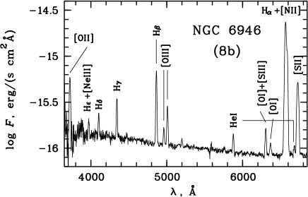
Figure 1: The ”b” spectrum of the eighth H II region of the galaxy.

Spectral observations were conducted in 2007 at the 6-m BTA telescope of the Special Astrophysical Observatory of the Russian Academy of Sciences (SAO RAS) with the SCORPIO focal reducer (for a detailed description of the device, see Afanasiev & Moiseev, 2005) in the multi-slit mode. The detector used was a CCD camera EEV 42-40. The size of the chip amounts to $2048\times 2048$ px, which provides a field of view of $6\hbox{${}^{\prime}$}$ given the image scale of $0.178\hbox{${}^{\prime\prime}$}$ per pixel. In the multi-slit mode the SCORPIO instrument has 16 movable slits, installed in the focal plane and relocating in the field of $2.9\hbox{${}^{\prime}$}\times 5.9\hbox{${}^{\prime}$}$. The size of the slits is $1.5\hbox{${}^{\prime\prime}$}\times 18\hbox{${}^{\prime\prime}$}$, the distance between the centers of adjacent slits amounts to $22\hbox{${}^{\prime\prime}$}$. The log of spectral observations at the BTA is given in Table 2.

During the observations we used the VPHG550G grism with the dispersion of 2.1Å/px and spectral resolution of 10Å. This grism allows to register the radiation in the range of 3100–-7300Å, where the range edges vary depending on the position of the slit. The spectral range of the grism allows to obtain the lines from [O ii]$\lambda$3727+$\lambda$3729Å  to [S ii]$\lambda$6717+$\lambda$6731Å  in one spectrum (Fig. 1).

The choice of the H II regions for spectral observations was made based on the images of the galaxy in the $B$ and H$\alpha$ filters, earlier obtained at the 1.5-m telescope of the Maidanak Observatory (Uzbekistan) with the angular resolution of about $1\hbox{${}^{\prime\prime}$}$ (unpublished data). We have selected the bright (both in the $B$ and H$\alpha$ bands) regions with the angular sizes from 2 to $5\hbox{${}^{\prime\prime}$}$, located in a wide range of galactocentric distances. For each of the three sets of slit positions, from six to eight 15-minute exposures were obtained (Table 2). After each exposure the slit positions were shifted rightwards-–leftwards along the slit in the increments of 20 px. This made it possible to obtain the spectra of several nearby H II regions in a single slit. However, due to the shifts the total time of exposure for a number of individual H II regions was less than the total exposure time, specified in Table 2.

For the standard reduction and data calibration, at the beginning and end of each set of observations of NGC 6946, the images with the zero exposure (bias), flat field, the spectra of the helium-neon-argon lamp and the comparison star were obtained.

Table 2: Log of spectral observations.

Date	Set of	Exposure,	Seeing,	Air
	slit	s	arcsec	mass
	positions
Sep 06, 2007	1	$900\times 6$	1.2	1.08
	2	$900\times 6$	1.2	1.57
Sep 07, 2007	3	$900\times 8$	1.6	1.19

2.2 Data Reduction

Further data reduction was carried out at the SAI MSU via a standard procedure using the ESO MIDAS image processing system. The main processing steps included: removal of traces of cosmic ray particles, identifying and correcting the data for the bias and flat field; conversion to the wavelength scale using the spectrum of a He-Ne-Ar lamp; normalization of fluxes by the intensity of the central (eighth) slit; background subtraction; conversion of the instrumental fluxes into absolute, using the observational data of spectrophotometric standard stars and the correction for the atmospheric extinction; the integration of two-dimensional spectra in the selected apertures for obtaining the one-dimensional spectra of the individual H II region; addition of spectra for each region. An example of the resulting spectrum is shown in Fig 1.

In the transition to one-dimensional spectra we integrated the two-dimensional spectra in the apertures, corresponding to the areas, where the bright emission lines of the H II regions were recognizable above the noise. The aperture size approximately corresponds to the diameter of an individual H II region along the slit position angle.

The continuum was predetermined and subtracted from the spectra to measure the fluxes in the emission lines. The star BD+25^∘4655 (Oke, 1990) was used as a spectrophotometric standard. To calculate the atmospheric extinction coefficient and correct for the atmospheric extinction, the results of astroclimatic measurements were used along with the observations of BD+25^∘4655 (Kartasheva & Chounakova, 1978). To separate the fluxes of the blended emission lines, they (the doublets or triplets) were simultaneously described by two or three Gaussians.

All in all, we have obtained the spectra of 39 H II regions (Fig. 2). The regions observed twice are marked in Tables 3, 4, 5 by letters ”a” and ”b” for the first and second obtained spectra, respectively.

The line intensity measurement errors include several components. The first source of errors is associated with the Poisson photon statistics in the line flux. The second component is caused by the error in determining the continuum level under the emission line and provides the main contribution to the total error for single lines. The third source of errors is associated with the accuracy of determining the spectral sensitivity curve, it is significant (over $1\%$) in the short-wavelength spectral region for the wavelengths of $\lambda<4000$Å. The last source of error, which is important for blended lines is due to the blend approximation errors by the Gaussians. The total error of line intensity was determined by quadratic summation of all the error components. These full errors were then correctly converted into the errors of calculated parameters by standard formulae.

Note that the absolute values of fluxes in the emission lines obtained for one and the same H II region may significantly differ from one set to another. This is caused by the seeing variation and the error of slit pointing on the object. Also note that the angular sizes of the observed H II regions are by 2–-3 times larger than the slit width, and the regions themselves can possess a complex internal structure. For these reasons the absolute values of fluxes, obtained for the H II regions observed twice may be very different from each other (see Table 3), while the line flux ratios for these regions are almost everywhere identical within the error margins (Table 4).

We estimated the equivalent widths (EW) of the H$\alpha$ and H$\beta$ emission lines from the spectra of H II regions, taking into account the continuum (Fig. 1). Such spectra were constructed by subtracting from the spectrum of the H II region the spectrum of the surrounding galactic disk background. This allows us to eliminate the contribution of stars and gas of the NGC 6946 disk in the radiation, coming from the H II region, and eliminates the problem of accounting for the contribution of the diffuse extraplanar ionized gas of the Galaxy, considered in detail by Efremov et al. (2011). For some H II regions the resulting level of the continuum appeared to by very small (close to zero), causing the obtained EW values to be unrealistically high, and the error estimates to be huge. Such data are not included in Table 3.

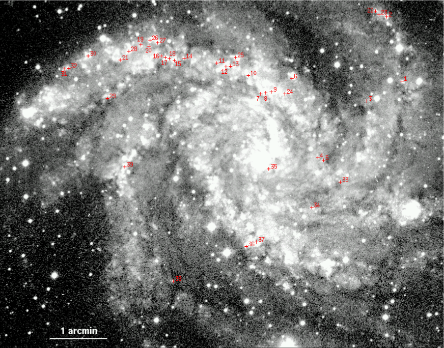
Figure 2: The image of the galaxy in the $B$-band. The positions of H II regions are marked. The numbers correspond to the index number of the region in Table 3. North is on top, east is to the left.

Table 3 lists the coordinates, deprojected galactocentric distances $r$, equivalent H$\alpha$ and H$\beta$ line widths and $F$(H$\beta$) fluxes of the H II regions, not corrected for absorption.

Table 4 lists the normalized for H$\beta$ and corrected for the interstellar extinction of light relative intensities of the [O ii]$\lambda$3727+$\lambda$3729Å, [O iii]$\lambda$5007Å, [N ii]$\lambda$6584Å, and [S ii]$\lambda$6717+$\lambda$6731Å  lines. The account of the extinction of the gas radiation emission lines was carried out by the observed values of the Balmer decrement in the spectra of the investigated objects. We used the theoretical ratio of the H$\alpha$/H$\beta$ lines from Osterbrock (1989) for the case B: recombination at the electron temperature of $10^{4}$ K, and analytical approximation of Izotov et al. (1994) of the Whitford interstellar reddening law. We took the equivalent width of the hydrogen absorption lines EW_a($\lambda$) to be equal to 2Å  for all objects. According to McCall et al. (1985), this value is the average for the H II regions. For the lines of other chemical elements EW_a($\lambda$) = 0.

Determining the errors of the corrected for interstellar extinction of light relative intensities of lines, presented in Table 4, we took into account the errors of intensity of the corresponding line, the H$\beta$ line, and the coefficient of absorption $c$(H$\beta$).

3 ANALYSIS

3.1 Abundance of Chemical Elements

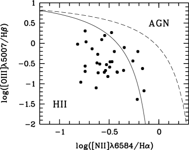
Figure 3: The BPT diagram for the H II regions, studied in the present paper (black circles). The solid line separating the classical H II regions from the objects with nonthermal emission spectra (AGN) is calculated according to Kewley et al. (2001). The dashed line is the curve, adopted from Kauffmann et al. (2003).

Take a look at the positions of our objects in the diagnostic BPT diagram (Fig. 3). The figure clearly shows that all the objects are located in the region, where the emission lines are emerging as a result of thermal radiation, implying that all the objects are the classical H II regions. Based on this, all these objects are taken for the further analysis of chemical elements.

Table 3: Parameters of the H II regions, equivalent widths of the H$\alpha$, H$\beta$ lines, and the H$\beta$ line fluxes.

H II	Set	Number from	Coordinates,	$r$,	EW(H$\beta$),	EW(H$\alpha$),	$F$(H$\beta$),
region		Belley & Roy (1992),	arcsec	kpc	Å	Å	10-16
		McCall et al. (1985),					erg/(s$\cdot$cm2)
		Ferguson et al. (1998)
1	1	116	79.7N, 146.5W	5.34	—	—	$6.63\pm 0.38$
2	1	143, 5	146.9N, 130.5W	6.51	$81.4\pm 3.4$	$519.0\pm 24.7$	$84.06\pm 1.33$
3	1	—	58.9N, 110.0W	3.99	$14.9\pm 5.4$	$106.5\pm 30.1$	$1.23\pm 0.20$
4	1	—	0.3S, 58.8W	1.75	$27.0\pm 3.5$	$105.6\pm 8.5$	$5.97\pm 0.23$
5a	1	—	2.7S, 64.6W	1.91	$15.8\pm 5.0$	$80.5\pm 13.9$	$1.85\pm 0.24$
5b	2	—	2.7S, 64.6W	1.91	$9.6\pm 1.7$	$61.2\pm 6.8$	$3.61\pm 0.33$
6	1	149	82.6N, 31.6W	2.95	$9.5\pm 0.4$	$92.2\pm 3.8$	$21.03\pm 0.60$
7	1	—	66.3N, 1.2E	2.14	$1.1\pm 0.4$	$37.2\pm 8.8$	$0.30\pm 0.07$
8a	1	1	67.7N, 4.1W	2.21	$27.9\pm 2.1$	$151.1\pm 11.4$	$8.86\pm 0.23$
8b	2	1	67.7N, 4.1W	2.21	$84.0\pm 4.3$	$645.8\pm 38.3$	$92.95\pm 1.52$
9	1	150	68.5N, 10.2W	2.28	$102.1\pm 6.0$	$939.3\pm 77.3$	$33.02\pm 0.54$
10	1	10	85.5N, 14.0E	2.75	$15.0\pm 0.8$	$117.7\pm 5.5$	$22.97\pm 0.65$
11	1	—	98.6N, 46.8E	3.32	$61.8\pm 8.6$	$577.0\pm 80.3$	$29.52\pm 0.84$
12	1	8	94.9N, 37.5E	3.13	$18.9\pm 0.8$	$173.9\pm 9.0$	$20.31\pm 0.43$
13	1	6	95.4N, 32.4E	3.12	$49.1\pm 5.7$	$264.3\pm 28.2$	$13.50\pm 0.40$
14	1	24	103.4N, 81.0E	3.87	$158.5\pm 25.9$	$997.9\pm 160.3$	$24.82\pm 0.45$
15a	1	25	101.0N, 91.4E	3.98	$103.9\pm 30.3$	$771.1\pm 273.9$	$13.75\pm 0.38$
15b	2	25	101.0N, 91.4E	3.98	$85.0\pm 19.7$	$525.6\pm 93.9$	$21.21\pm 0.67$
16	1	29	106.1N, 105.0E	4.34	$136.0\pm 53.2$	$664.4\pm 134.7$	$19.44\pm 0.58$
17	1	28	104.2N, 101.0E	4.22	$50.2\pm 4.6$	$385.0\pm 26.7$	$17.14\pm 0.37$
18	2	26	103.1N, 96.7E	4.12	$44.3\pm 4.2$	$179.7\pm 11.9$	$27.25\pm 0.65$
19	1	16	117.8N, 126.3E	5.00	$113.2\pm 13.7$	$1055.1\pm 107.0$	$23.54\pm 0.43$
20	1	—	116.2N, 118.0E	4.81	—	—	$10.67\pm 0.36$
21	1	19	101.8N, 147.6E	5.14	$107.7\pm 21.7$	$570.4\pm 55.1$	$48.75\pm 1.11$
22	2	146	153.0N, 118.8W	6.44	$113.9\pm 22.8$	$304.3\pm 14.4$	$17.37\pm 0.46$
23	2	145	149.3N, 122.5W	6.41	$73.6\pm 9.0$	$333.7\pm 28.6$	$16.56\pm 0.38$
24	2	151	66.3N, 23.8W	2.35	$8.5\pm 3.0$	$30.4\pm 3.5$	$4.00\pm 0.87$
25	2	5	104.5N, 27.1E	3.38	$39.7\pm 2.7$	$416.9\pm 35.1$	$39.02\pm 0.88$
26	2	15	122.3N, 116.7E	4.92	$27.5\pm 1.2$	$158.5\pm 6.5$	$26.38\pm 0.49$
27	2	14	119.9N, 108.7E	4.72	$92.8\pm 8.7$	$691.4\pm 47.4$	$59.51\pm 1.03$
28	2	17	110.6N, 138.6E	5.10	$7.1\pm 1.2$	$113.0\pm 15.4$	$4.05\pm 0.34$
29	2	—	61.8N, 161.2E	4.95	$13.3\pm 2.1$	$114.8\pm 12.5$	$9.55\pm 0.65$
30	2	39, 4, A	105.8N, 181.2E	6.00	$83.9\pm 3.4$	$560.4\pm 15.1$	$144.84\pm 2.28$
31	2	—	92.5N, 206.3E	6.47	$31.4\pm 4.2$	$315.8\pm 56.9$	$9.68\pm 0.35$
32	2	—	93.3N, 201.5E	6.35	$13.8\pm 1.1$	$131.5\pm 7.5$	$8.55\pm 0.31$
33	3	—	25.7S, 82.0W	2.47	$59.8\pm 29.6$	$292.1\pm 95.9$	$8.90\pm 0.86$
34	3	—	52.6S, 52.4W	2.16	$23.0\pm 1.3$	$208.5\pm 15.3$	$33.43\pm 0.78$
35	3	163	12.1S, 7.6W	0.43	$6.1\pm 0.7$	$38.4\pm 2.3$	$6.39\pm 0.46$
36	3	78	92.9S, 15.9E	3.10	$14.7\pm 0.8$	$117.2\pm 5.7$	$42.23\pm 1.12$
37	3	—	88.1S, 5.5E	2.88	$6.9\pm 1.9$	$83.7\pm 13.0$	$2.83\pm 0.36$
38	3	—	129.1S, 92.4E	5.29	—	—	$4.63\pm 0.16$
39	3	49, 3	9.7S, 142.8E	4.30	$56.2\pm 3.3$	$399.9\pm 21.1$	$81.34\pm 1.46$

A number of empirical correlations between the relative intensities of emission lines and the chemical composition and temperature of the emitting gas have been proposed at different times by many researchers (see the surveys Ellison et al., 2008; López-Sánchez & Esteban, 2010). Let us outline among them two recent calibrations used to determine the metallicity in the H II regions. Both the ON- (Pilyugin et al., 2010) and NS-calibrations (Pilyugin & Mattsson, 2011) interpret the relative intensities of strong emission lines (O²⁺, O⁺, and N⁺ in the case of ON-calibration or O²⁺, N⁺, and S⁺ in the case of NS-calibration) in terms of the relative oxygen and nitrogen abundances and electron temperatures. Since the relative intensities of [O ii]$\lambda$3727+$\lambda$3729/H$\beta$ were measured with large errors, or have not been measured at all in many objects, we chose the NS-calibration to determine the metallicity and electron temperature of the gas in the studied H II regions.

As the [O iii]$\lambda$4959Å  line intensities were measured by us only for a half of H II regions, and the [N ii]$\lambda$6548Å  line intensities were determined with very high errors, in the calculation of the oxygen and nitrogen abundances, and electron temperature, we used the following ratios: [O iii]$\lambda$4959+$\lambda$5007Å=1.33[O iii]$\lambda$5007Å  and [N ii]$\lambda$6548+$\lambda$6584Å=1.33[N ii]$\lambda$6584Å  (following Storey & Zeippen, 2000).

The NS-method is applicable to the regions of low density. Unfortunately, the sulfur [S ii]$\lambda$6717Å  and [S ii]$\lambda$6731Å  doublet lines are blended in our spectra and can only be isolated with a poor accuracy. Hence, we could not confidently determine the density of the studied objects. Nevertheless, for all the studied H II regions, [S ii]$\lambda$6717Å/[S ii]$\lambda$6731Å$\geq$1 (Table 4), what corresponds to the density values of $N_{e}\leq 300$ cm^-3. Thus, the estimates show that all our objects have low densities, which is typical of giant H II regions, observed in other galaxies (Kennicutt, 1984; Zaritsky et al., 1994; Bresolin et al., 2005; Gutiérrez & Beckman, 2010).

The estimates of metallicity and electron temperature, obtained using the NS-calibration in our sample are given in Table 5. For the NS-calibration we used the spectra of H II regions with reliable estimates of electron temperature (Pilyugin & Mattsson, 2011). Therefore, the metallicity estimates are in a good agreement with the values given by the classical $T_{e}$-method (see Fig. 4). It is clear from the O/H––N/O diagram (Fig. 4) that the objects we have studied in the NGC 6946 are within the lane, occupied by the most reliably investigated H II regions in other galaxies. This agreement indicates the validity of metallicity estimates obtained for the studied objects.

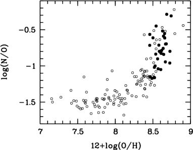
Figure 4: The O/H–-N/O diagram. The open circles represent a sample of well-studied H II regions in the nearby galaxies from Pilyugin et al. (2010), black circles are the objects studied in this paper.

Table 4: The absorption coefficients $c$(H$\beta$), emission line fluxes corrected for reddening (in the units of $I$(H$\beta$)) and the ratio of sulfur lines [S ii]6717Å/[S ii]6731Å.

H II	$c$(H$\beta$)	[O ii]	[O iii]	[N ii]	[S ii]	[S ii]6717Å/
region		3727+3729Å	5007Å	6584Å	6717+6731Å	[S ii]6731Å
1	1.26$\pm$0.12	—	0.11$\pm$0.03	0.47$\pm$0.12	0.54$\pm$0.11	1.49$\pm$0.44
2	1.80$\pm$0.04	—	0.79$\pm$0.03	1.29$\pm$0.11	0.76$\pm$0.05	1.20$\pm$0.18
3	0.54$\pm$0.34	—	—	1.29$\pm$0.67	1.02$\pm$0.51	2.54$\pm$1.31
4	0.19$\pm$0.09	—	—	1.04$\pm$0.17	0.47$\pm$0.09	4.80$\pm$3.69
5a	0.83$\pm$0.28	—	—	0.96$\pm$0.44	0.45$\pm$0.21	—
5b	0.68$\pm$0.21	—	—	0.74$\pm$0.28	—	—
6	0.90$\pm$0.07	—	0.35$\pm$0.04	0.97$\pm$0.13	0.56$\pm$0.07	1.55$\pm$0.33
7	1.57$\pm$0.72	—	—	3.31$\pm$3.10	—	—
8a	0.60$\pm$0.07	—	0.21$\pm$0.03	0.83$\pm$0.12	0.65$\pm$0.07	1.20$\pm$0.26
8b	0.95$\pm$0.05	1.68$\pm$0.21	0.29$\pm$0.01	0.85$\pm$0.10	0.65$\pm$0.04	1.02$\pm$0.17
9	1.11$\pm$0.05	1.23$\pm$0.20	0.21$\pm$0.01	0.52$\pm$0.08	0.51$\pm$0.03	1.09$\pm$0.21
10	0.96$\pm$0.07	—	0.04$\pm$0.02	1.73$\pm$0.20	0.62$\pm$0.07	1.56$\pm$0.31
11	0.92$\pm$0.07	—	0.07$\pm$0.02	2.03$\pm$0.21	0.67$\pm$0.07	0.95$\pm$0.16
12	1.12$\pm$0.06	—	—	0.80$\pm$0.10	0.55$\pm$0.05	1.87$\pm$0.49
13	1.38$\pm$0.07	—	0.24$\pm$0.03	1.97$\pm$0.22	0.82$\pm$0.10	1.38$\pm$0.31
14	1.57$\pm$0.05	—	0.19$\pm$0.02	0.81$\pm$0.09	0.46$\pm$0.04	1.62$\pm$0.32
15a	1.06$\pm$0.07	—	0.35$\pm$0.04	0.92$\pm$0.12	0.83$\pm$0.09	1.18$\pm$0.21
15b	1.01$\pm$0.07	—	0.33$\pm$0.04	0.68$\pm$0.10	0.29$\pm$0.04	1.18$\pm$0.28
16	1.76$\pm$0.07	—	0.20$\pm$0.03	1.09$\pm$0.13	0.51$\pm$0.06	1.34$\pm$0.24
17	1.81$\pm$0.06	—	0.22$\pm$0.02	1.26$\pm$0.12	0.50$\pm$0.04	1.12$\pm$0.17
18	0.63$\pm$0.06	—	0.27$\pm$0.03	0.52$\pm$0.08	0.71$\pm$0.06	1.64$\pm$0.30
19	1.40$\pm$0.05	—	0.53$\pm$0.02	0.69$\pm$0.07	0.38$\pm$0.03	1.26$\pm$0.17
20	1.07$\pm$0.07	—	0.63$\pm$0.05	1.02$\pm$0.13	1.21$\pm$0.13	1.21$\pm$0.17
21	1.06$\pm$0.05	1.04$\pm$0.27	0.31$\pm$0.02	0.73$\pm$0.08	0.54$\pm$0.04	1.43$\pm$0.18
22	2.15$\pm$0.06	—	1.09$\pm$0.06	0.53$\pm$0.07	0.21$\pm$0.02	2.59$\pm$0.66
23	1.27$\pm$0.06	—	0.63$\pm$0.04	1.76$\pm$0.17	0.80$\pm$0.07	1.59$\pm$0.29
24	0.18$\pm$0.45	—	—	1.25$\pm$0.82	1.24$\pm$0.91	2.04$\pm$0.94
25	1.20$\pm$0.06	—	0.19$\pm$0.02	0.70$\pm$0.09	0.61$\pm$0.05	1.83$\pm$0.38
26	0.75$\pm$0.05	—	0.74$\pm$0.03	0.61$\pm$0.07	0.64$\pm$0.05	1.46$\pm$0.24
27	1.08$\pm$0.04	—	0.95$\pm$0.03	0.44$\pm$0.05	0.36$\pm$0.03	1.47$\pm$0.24
28	1.19$\pm$0.19	—	1.83$\pm$0.27	0.96$\pm$0.29	1.28$\pm$0.37	1.85$\pm$0.56
29	0.85$\pm$0.15	—	—	0.93$\pm$0.22	0.90$\pm$0.22	1.70$\pm$0.45
30	1.11$\pm$0.04	0.92$\pm$0.11	2.02$\pm$0.05	0.52$\pm$0.05	0.51$\pm$0.03	1.46$\pm$0.18
31	0.59$\pm$0.08	—	1.24$\pm$0.08	0.76$\pm$0.11	0.90$\pm$0.11	1.36$\pm$0.19
32	1.25$\pm$0.08	—	1.56$\pm$0.11	0.82$\pm$0.12	0.93$\pm$0.11	1.49$\pm$0.22
33	0.78$\pm$0.19	—	0.36$\pm$0.08	1.57$\pm$0.44	0.90$\pm$0.28	2.19$\pm$0.95
34	1.04$\pm$0.06	—	0.19$\pm$0.03	1.09$\pm$0.12	0.45$\pm$0.05	1.55$\pm$0.35
35	1.57$\pm$0.17	—	—	1.80$\pm$0.45	0.74$\pm$0.21	3.10$\pm$1.98
36	0.65$\pm$0.07	1.72$\pm$0.43	0.08$\pm$0.02	0.67$\pm$0.10	0.61$\pm$0.06	1.44$\pm$0.28
37	0.77$\pm$0.29	—	—	0.70$\pm$0.33	0.49$\pm$0.25	1.87$\pm$1.58
38	0.25$\pm$0.08	—	0.26$\pm$0.05	0.92$\pm$0.13	0.38$\pm$0.06	0.97$\pm$0.29
39	1.25$\pm$0.05	—	0.15$\pm$0.01	0.88$\pm$0.08	0.71$\pm$0.04	1.46$\pm$0.19

3.2 Comparison of Results with Previous Studies

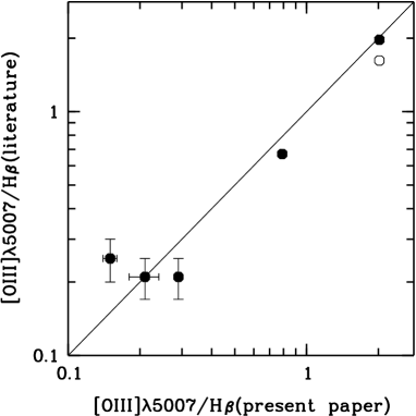
Figure 5: A comparison of relative fluxes in the line of oxygen [O iii]$\lambda$5007Å, obtained in the present work with the data from McCall et al. (1985) (black circles) and Ferguson et al. (1998) (open circles) for common objects. The measurement errors, not exceeding the sizes of the signs in the figure are not shown.

We compared our estimates of relative intensity of the H II region emission lines in the galaxy with the results from McCall et al. (1985); Ferguson et al. (1998). Four objects from our sample (one of which was observed twice) coincide with the H II regions from the list of McCall et al. (1985), one of these objects was also studied in Ferguson et al. (1998) (Table 3). For the reasons stated in the introduction, we did not compare our results with the spectrophotometric data (Belley & Roy, 1992). Fig. 5 in a way of example gives a comparison of relative fluxes in the [O iii]$\lambda$5007Å  line for the coinciding objects that were obtained by us and in McCall et al. (1985); Ferguson et al. (1998). The figure demonstrates a satisfactory agreement between them.

The differences between our results and those obtained by McCall et al. (1985); Ferguson et al. (1998), which are for some objects higher than the measurement errors, may be caused by the fact that the angular scales of the H II regions in the nearby NGC 6946 galaxy are as a rule greater than the width of the slit, set for the spectroscopic observations. Different authors obtain the spectra of various parts of the H II region with a slightly different chemical composition. Also note the problem, associated with the identification of H II regions in the given stellar system: NGC 6946 is an example of a galaxy with a virtually complete absence of large stellar complexes. Its spiral arms are the chains of closely spaced H II regions. A slightly different seeing during the observations may result in the differences in the definition of what actually constitutes an individual H II region.

3.3 Metallicity Gradient, Electron Temperature

The metallicity variations in the H II regions, depending on their galactocentric distance reflect the chemical evolution of the disk galaxies. To investigate the metallicity gradient in the galactic disk we need a sample of H II regions, relatively evenly distributed over the galactocentric distances. Such samples of H II regions with measured chemical compositions are available only for a limited number (about 50) of nearby galaxies (see the following surveys: Garnett, 2002; Pilyugin et al., 2004; Moustakas et al., 2010). We used the sample of 30 objects investigated in this study to determine the metallicity gradient in the disk of NGC 6946.

Table 5: The oxygen, nitrogen abundances and electron temperature in the H II regions.

H II	$r/R_{25}$	12+	12+	$t_{\rm NS}$,
regions		$\log$(O/H)	$\log$(N/H)	$10^{4}$ K
1	0.40	8.73$\pm$0.04	7.77$\pm$0.05	0.64$\pm$0.01
2	0.49	8.46$\pm$0.01	7.74$\pm$0.02	0.81$\pm$0.01
6	0.22	8.58$\pm$0.02	7.87$\pm$0.03	0.72$\pm$0.01
8a	0.17	8.62$\pm$0.02	7.83$\pm$0.03	0.69$\pm$0.01
8b	0.17	8.59$\pm$0.01	7.79$\pm$0.03	0.72$\pm$0.01
9	0.17	8.67$\pm$0.03	7.73$\pm$0.05	0.68$\pm$0.01
10	0.21	8.74$\pm$0.05	8.43$\pm$0.02	0.58$\pm$0.02
11	0.25	8.68$\pm$0.03	8.40$\pm$0.01	0.61$\pm$0.01
13	0.23	8.54$\pm$0.02	8.09$\pm$0.03	0.71$\pm$0.01
14	0.29	8.67$\pm$0.02	7.97$\pm$0.02	0.66$\pm$0.01
15a	0.30	8.54$\pm$0.02	7.70$\pm$0.03	0.75$\pm$0.01
15b	0.30	8.68$\pm$0.02	7.98$\pm$0.04	0.67$\pm$0.01
16	0.33	8.64$\pm$0.02	8.05$\pm$0.03	0.67$\pm$0.01
17	0.32	8.63$\pm$0.02	8.11$\pm$0.03	0.67$\pm$0.01
18	0.31	8.60$\pm$0.02	7.55$\pm$0.04	0.72$\pm$0.01
19	0.38	8.60$\pm$0.01	7.80$\pm$0.03	0.73$\pm$0.01
20	0.36	8.52$\pm$0.02	7.36$\pm$0.05	0.79$\pm$0.01
21	0.39	8.61$\pm$0.01	7.78$\pm$0.02	0.71$\pm$0.01
22	0.48	8.56$\pm$0.02	7.66$\pm$0.05	0.78$\pm$0.01
23	0.48	8.46$\pm$0.01	7.89$\pm$0.03	0.79$\pm$0.01
25	0.25	8.64$\pm$0.02	7.80$\pm$0.03	0.68$\pm$0.01
26	0.37	8.52$\pm$0.01	7.50$\pm$0.03	0.80$\pm$0.01
27	0.36	8.57$\pm$0.01	7.53$\pm$0.03	0.78$\pm$0.01
28	0.38	8.53$\pm$0.05	7.53$\pm$0.12	0.87$\pm$0.02
30	0.45	8.47$\pm$0.02	7.32$\pm$0.04	0.88$\pm$0.01
31	0.49	8.49$\pm$0.02	7.32$\pm$0.04	0.84$\pm$0.01
32	0.48	8.52$\pm$0.02	7.36$\pm$0.05	0.85$\pm$0.01
33	0.19	8.50$\pm$0.05	7.89$\pm$0.09	0.75$\pm$0.02
34	0.16	8.66$\pm$0.02	8.10$\pm$0.02	0.66$\pm$0.01
36	0.23	8.73$\pm$0.03	7.93$\pm$0.02	0.63$\pm$0.01
38	0.40	8.66$\pm$0.03	8.05$\pm$0.04	0.67$\pm$0.01
39	0.32	8.64$\pm$0.01	7.88$\pm$0.02	0.67$\pm$0.01

The study of the radial distribution of nitrogen in galaxies is generally given less attention than the research of the O/H gradient. However, the knowledge of the radial N/H gradient is important for the study of the chemical evolution of galaxies. Starting from the values of $12+\log({\rm O/H})\geq 8.3$ the secondary nitrogen begins to dominate in the gas disk. Its abundance increases more rapidly than the oxygen content (Henry et al., 2000). As a result, the variations of the nitrogen abundance with distance from the center of the galaxy has a greater amplitude than the variation in the oxygen content, and can be determined with a good accuracy, despite the fact that the fluxes in the nitrogen lines are usually measured with larger errors than those in the lines of oxygen. In addition, a comparative analysis of the O/H and N/H gradients in the galaxy can provide information on the delay of appearance of nitrogen in the interstellar medium with respect to oxygen (Maeder, 1992; van den Hoek & Groenewegen, 1997; Pagel, 1997; Pilyugin & Thuan, 2011). Therefore, we determine here the radial gradients of both oxygen and nitrogen.

Radial distributions of metallicity are generally described by the following expressions:

$$12+\log({\rm O/H})=12+\log({\rm O/H})_{0}+C_{\rm O/H}\times(r/R_{25}),$$ (1)

where $12+\log({\rm O/H})_{0}$ is the relative abundance of oxygen, extrapolated to the center, $C_{\rm O/H}$ is the value of gradient of the radial decrease of relative oxygen abundance in the units of dex/$R_{\rm 25}$, $r$/$R_{\rm 25}$ is the galactocentric distance in the units of the galactic radius, measured from the isophote 25^m/arcsec² (Zaritsky et al., 1994; van Zee et al., 1998; Pilyugin et al., 2004). The radial distribution of relative nitrogen content is described similarly:

$$12+\log({\rm N/H})=12+\log({\rm N/H})_{0}+C_{\rm N/H}\times(r/R_{25}).$$ (2)

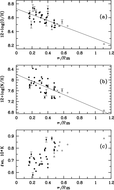
Figure 6: The diagrams of radial distribution of the relative abundance of oxygen (a), nitrogen (b) and the values of electron temperature $t_{\rm NS}$ (c) in the disk of NGC 6946. The open circles denote the objects, measured in McCall et al. (1985), the open triangles are the measurements from Ferguson et al. (1998), the oblique crosses — García-Benito et al. (2010), while the black circles are the objects studied in this paper. The values determined with an accuracy of less than $\pm 0.02$ dex (a), $\pm 0.04$ dex (b) and $\pm 100$ K (c) are accompanied with the error bars. The straight lines describe the radial gradient of the oxygen and nitrogen abundances.

Figs. 6a and  6b show the radial distribution of relative oxygen and nitrogen abundances in the disk of NGC 6946, respectively. We can see that the actual spread of metallicity at a fixed radius exceeds the chemical composition measurement errors. The objects from McCall et al. (1985); Ferguson et al. (1998) are also subject to this spread: one of the objects from the samples of McCall et al. (1985); Ferguson et al. (1998) is identified with the object no. 30 from our sample and has the same chemical composition.

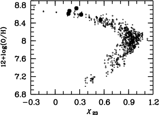
Figure 7: The $X_{23}$–O/H diagram for the sample of H II regions according to Pilyugin et al. (2010) (dots), Pilyugin et al. (2012) (gray dots), and five objects investigated in the present study (black circles).

The numerical values of the sought coefficients in the expressions (1) and (2) were determined via the least squares method for all the objects shown in Fig. 6. We obtained the following values of the coefficients:
$12+\log({\rm O/H})_{0}=8.73\pm 0.02$,
$C_{\rm O/H}=-0.43\pm 0.06$ dex/$R_{\rm 25}$,
$12+\log({\rm N/H})_{0}=8.21\pm 0.08$,
$C_{\rm N/H}=-1.25\pm 0.19$ dex/$R_{\rm 25}$.

Fig. 6 shows that the radial distributions of the oxygen and nitrogen abundances are described by a single regression model throughout the entire disk of NGC 6946. The distribution of the nitrogen abundance varies faster relative to the radial distribution of oxygen.

The galaxy reveals an increase in the electron temperature of the H II regions with distance from the galactic center (Fig. 6c). A similar dependence is also observed for the H II regions in the Galaxy (Churchwell et al., 1978; Paladini et al., 2004; Quireza et al., 2006; Balser et al., 2011). The temperature–-metallicity dependence for the H II regions in NGC 6946 is rather well explained by the theoretical models of Rubin (1985).

4 DISCUSSION

Figs. 6a and  6b show a large dispersion of object positions relative to the regression model of the radial gradient of chemical composition. This is consistent with the results of previous studies (McCall et al., 1985; Ferguson et al., 1998; García-Benito et al., 2010) for the common and nearby objects. McCall et al. (1985); Ferguson et al. (1998) have investigated the abundance of chemical elements in the MRS 4 (+182, +103) = FGW 6946A complex (corresponds to the complex 30 from our list), and obtained the metallicities, which coincide with our values within the errors (Fig. 6). On the northern edge of the spiral arm (the eastern part of the galaxy) a giant stellar complex is located, it was investigated in García-Benito et al. (2010) and denominated as Knot A. The estimations of the oxygen and nitrogen abundances in the complex, obtained in García-Benito et al. (2010), proved to be similar ($12+\log{\rm(O/H)}=8.48\pm 0.01$, $12+\log{\rm(N/H)}=7.38\pm 0.01$) with the O/H and N/H estimates, obtained in the present work for the most nearby to the Knot A regions number 31 and 32 (Figs. 2, 6, Table 5).

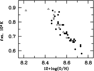
Figure 8: The dependence of the electron temperature on the relative abundance of oxygen in the H II regions. The designations are the same as in Fig. 6.

A large dispersion is most likely due to the conditions of observations of the H II regions in this galaxy. NGC 6946 is a sufficiently close galaxy, and the nebulae in it have relatively large angular dimensions. In the case if the spectrograph slit has only captured the central part of the nebula, where the nitrogen is doubly ionized, the NS-calibration used here leads to an underestimation of the oxygen content. If the spectrograph slit captures the peripheral part of the nebula, where the doubly ionized nitrogen is absent, the NS-calibration yields an exaggerated oxygen abundance. In order to test the reliability of the obtained oxygen abundance estimates, we checked the positions of the investigated objects on other diagrams.

Based on the usual assumption that in the H II regions having similar intensities of strong emission lines there should be approximately the same physical conditions and chemical composition, we have compared in Fig. 7 the positions of objects, studied in this research (the black circles) with a sample of calibration areas from Pilyugin et al. (2010) (the black dots). The gray dots show the H II regions for which the oxygen abundance was determined via the recently proposed C-method (Pilyugin et al., 2012). We determined the parameter $X_{23}\equiv\log R_{23}\equiv\log$ (([O ii]$\lambda$3727+ $\lambda$3729Å+[O iii]$\lambda$4959Å+[O iii]$\lambda$5007Å)/H$\beta$) for five H II regions in NGC 6946, where we were able to measure the [O ii]$\lambda$3727+$\lambda$3729Å  line (Table 4) as $\log$ (([O ii]$\lambda$3727+$\lambda$3729Å+1.33[O iii]$\lambda$5007Å)/H$\beta$).

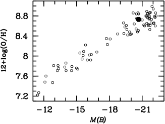
Figure 9: The luminosity–-central metallicity diagram. The open circles represent the data from Pilyugin et al. (2007) (with the addition of the results from Gusev et al., 2012), the black circle marks the position of NGC 6946 according to this paper.

Fig. 8 examines the relationship between the electron temperature and oxygen abundance in the studied regions, indicating that the electron temperature in the nebula essentially depends on the cooling of gas via irradiation in the oxygen lines. Here, like in Fig. 6c, a significantly underestimated electron temperature of the object from the sample of Ferguson et al. (1998) can be seen. Since this object was located far at the edge of the galactic disk ($R/R_{25}>1$), the account of this object can effect the choice of the radial the gradient of chemical composition of the galaxy. Without this object the gradient becomes a little flatter, $-0.39\pm 0.08$ dex/$R_{\rm 25}$ in the case of radial distribution of oxygen, and a little steeper $-1.30\pm 0.22$ dex/$R_{\rm 25}$ in the case of radial distribution of nitrogen.

The luminosity -– central metallicity diagram was built by Pilyugin et al. (2007). The oxygen and nitrogen abundances in Pilyugin et al. (2007) and in the present work were determined using the methods that are consistent with the metallicity scale, based on the $T_{e}$ method, hence they can be compared. Fig. 9 demonstrates the position of the central metallicity estimates of NGC 6946 obtained here compared with other galaxies. It is clear from the graph that the central metallicity obtained in this work is typical for the galaxy of a given luminosity.

5 CONCLUSIONS

Using the SCORPIO focal reducer in the multislit mode we have performed the spectroscopy of 39 H II regions of the NGC 6946 galaxy. The estimates of absorption were obtained for these regions.

Having applied the ”strong line” method the electron temperatures, oxygen and nitrogen abundances were determined for 30 H II regions. The radial gradients of O/H, N/H, and the electron temperature were constructed.

The radial decrease of the oxygen and nitrogen abundances amounted to
$12+\log({\rm O/H})=(8.73\pm 0.02)-(0.43\pm 0.06)r/R_{\rm 25}$ and
$12+\log({\rm N/H})=(8.21\pm 0.08)-(1.25\pm 0.19)r/R_{\rm 25}$.