A Unified Approach to Structural Limits and Limits of Graphs with Bounded Tree-depth

Abstract.

In this paper we introduce a general framework for the study of limits of relational structures and graphs in particular, which is based on a combination of model theory and (functional) analysis. We show how the various approaches to graph limits fit to this framework and that they naturally appear as “tractable cases” of a general theory. As an outcome of this, we provide extensions of known results. We believe that this puts these into a broader context. The second part of the paper is devoted to the study of sparse structures. First, we consider limits of structures with bounded diameter connected components and we prove that in this case the convergence can be “almost” studied component-wise. We also propose the structure of limit objects for convergent sequences of sparse structures. Eventually, we consider the specific case of limits of colored rooted trees with bounded height and of graphs with bounded tree-depth, motivated by their role as “elementary bricks” these graphs play in decompositions of sparse graphs, and give an explicit construction of a limit object in this case. This limit object is a graph built on a standard probability space with the property that every first-order definable set of tuples is measurable. This is an example of the general concept of modeling we introduce here. Our example is also the first “intermediate class” with explicitly defined limit structures where the inverse problem has been solved.

Chapter 1 Introduction

To facilitate the study of the asymptotic properties of finite graphs (and more generally of finite structures) in a sequence $G_{1},G_{2},\ldots,G_{n},\ldots$, it is natural to introduce notions of structural convergence. By structural convergence, we mean that we are interested in the characteristics of a typical vertex (or group of vertices) in the graph $G_{n}$, as $n$ grows to infinity. This convergence can be concisely expressed by various means. We note two main directions:

• the convergence of the sampling distributions;

• the convergence with respect to a metric in the space of structures (such as the cut metric).

Also, sampling from a limit structure may also be used to define a sequence convergent to the limit structure.

All these directions lead to a rich theory which originated in a probabilistic context by Aldous [3] and Hoover [48] (see also the monograph of Kallenberg [53] and the survey of Austin [8]) and, independently, in the study of random graph processes, and in analysis of properties of random (and quasirandom) graphs (in turn motivated among others by statistical physics [16, 17, 63]). This development is nicely documented in the recent monograph of Lovász [62].

The asymptotic properties of large graphs are studied also in the context of decision problems as exemplified e.g. by structural graphs theory, [26, 80]. However it seems that the existential approach typical for decision problems, structural graph theory and model theory on the one side and the counting approach typical for statistics and probabilistic approach on the other side have little in common and lead to different directions: on the one side to study, say, definability of various classes and the properties of the homomorphism order and on the other side, say, properties of partition functions. It has been repeatedly stated that these two extremes are somehow incompatible and lead to different areas of study (see e.g. [15, 46]). In this paper we take a radically different approach which unifies these both extremes.

We propose here a model which is a mixture of the analytic, model theoretic and algebraic approach. It is also a mixture of existential and probabilistic approach. Precisely, our approach is based on the Stone pairing $\langle\phi,G\rangle$ of a first-order formula $\phi$ (with set of free variables ${\rm Fv}(\phi)$) and a graph $G$, which is defined by the following expression

$$\langle\phi,G\rangle=\frac{|\{(v_{1},\dots,v_{|{\rm Fv}(\phi)|})\in G^{|{\rm Fv}(\phi)|}:G\models\phi(v_{1},\dots,v_{|{\rm Fv}(\phi)|})\}|}{|G|^{|{\rm Fv}(\phi)|}}.$$

Stone pairing induces a notion of convergence: a sequence of graphs $(G_{n})_{n\in\mathbb{N}}$ is ${\rm FO}$-convergent if, for every first order formula $\phi$ (in the language of graphs), the values $\langle\phi,G_{n}\rangle$ converge as $n\rightarrow\infty$. In other words, $(G_{n})_{n\in\mathbb{N}}$ is ${\rm FO}$-convergent if the probability that a formula $\phi$ is satisfied by the graph $G_{n}$ with a random assignment of vertices of $G_{n}$ to the free variables of $\phi$ converges as $n$ grows to infinity. We also consider analogously defined $X$-convergence, where $X$ is a fragment of ${\rm FO}$.

Our main result is that this model of FO-convergence is a suitable model for the analysis of limits of sparse graphs (and particularly of graphs with bounded tree depth). This fits to a broad context of recent research.

For graphs, and more generally for finite structures, there is a class dichotomy: nowhere dense and somewhere dense [78, 74]. Each class of graphs falls in one of these two categories. Somewhere dense class ${\mathcal{C}}$ may be characterised by saying that there exists a (primitive positive) FO interpretation of all graphs into them. Such class ${\mathcal{C}}$ is inherently a class of dense graphs. In the theory of nowhere dense structures [80] there are two extreme conditions related to sparsity: bounded degree and bounded diameter. Limits of bounded degree graphs have been studied thoroughly [10], and this setting has been partially extended to sparse graphs with far away large degree vertices [65]. The class of graphs with bounded diameter is considered in Section 3.3 (and leads to a difficult analysis of componentwise convergence). This analysis provides a first-step for the study of limits of graphs with bounded tree-depth. Classes of graphs with bounded tree-depth can be defined by logical terms as well as combinatorially in various ways; the most concise definition is perhaps that a class of graphs has bounded tree depth if and only if the maximal length of a path in every $G$ in the class is bounded by a constant. Graphs with bounded tree-depth play also the role of building blocks of graphs in a nowhere dense class (by means of low tree-depth decompositions [68, 69, 80]). So the solution of limits for graphs with bounded tree depth presents a step (and perhaps provides a road map) in solving the limit problem for sparse graphs.

We propose here a new type of measurable structure, called modeling, which extends the notion of graphing, and which we believe is a good candidate for limit objects of sequence of graphs in a nowhere dense class. The convergence of graphs with bounded tree depth is analysed in detail and this leads to a construction of a modeling limits for those sequences of graphs where all members of the sequence have uniformly bounded tree depth (see Theorem 4.36). Moreover, we characterize modelings which are limits of graphs with bounded tree-depth.

There is more to this than meets the eye: We prove that if ${\mathcal{C}}$ is a monotone class of graphs such that every ${\rm FO}$-convergent sequence has a modeling limit then the class ${\mathcal{C}}$ is nowhere dense (see Theorem 1.8). This shows the natural limitations to modeling ${\rm FO}$-limits. To create a proper model for bounded height trees we have to introduce the model in a greater generality and it appeared that our approach relates and in most cases generalizes, by properly choosing a fragment $X$ of ${\rm FO}$, all existing models of graph limits. For instance, for the fragment $X$ of all existential first-order formulas, $X$-convergence means that the probability that a structure has a particular extension property converges. Our approach is encouraged by the deep connections to the four notions of convergence which have been proposed to study graph limits in different contexts.

The ultimate goal of the study of structural limits is to provide (as effectively as possible) limit objects themselves: we would like to find an object which will induce the limit distribution and encode the convergence.

For dense graphs Lovász and Szegedy managed to unveil the essential notion of a graphon, which exactly fits their notion of convergence: In this representation the limit [63, 16] is a symmetric Lebesgue measurable function $W:[0,1]^{2}\rightarrow[0,1]$ called a graphon and every graphon is the limit of a sequence of graphs. Such a representation is of course not unique, in the sense that different graphons may define the same graph limit, but equivalence of graphons is well understood [13, 25]. A connection between graph limits and de Finetti’s theorem for exchangeable arrays (and the early works of Aldous [3], Hoover [48] and Kallenberg [53]) has been established, see e.g. Diaconis and Janson [25]. Note that representation of graph limits by graphons extend (in a non-trivial way) to regular hypergraphs [32, 91] and, more generally, to relational structures [6, 7].

A representation of the limit for our second example of bounded degree graphs is a measurable graphing (notion introduced by Adams [1] in the context of Ergodic theory), that is a standard Borel space with a measure $\mu$ and $d$ measure preserving Borel involutions. The existence of such a representation has been made explicit by Elek [31], and relies on the works of Benjamini [10] and Gaboriau [38]. Graphing representation is not unique, but the equivalence of graphings (called local equivalence) can be characterized by means of bi-local isomorphism [62]. However, it is a difficult open problem, known as Aldous–Lyons conjecture, whether every graphing is the limit of some sequence of finite graphs (see Conjecture 1.2).

Both of these models of convergence are particular cases of our general approach. One of the main issue of our general approach is to determine a representation of ${\rm FO}$-limits as measurable graphs. A natural limit object is a standard probability space $(V,\Sigma,\mu)$ together with a graph with vertex set $V$ and edge set $E$, with the property that every first-order definable subset of a power of $V$ is measurable. This leads to the notion of relational sample space and to the notion of modeling. This notion seems to be particularly suitable for sparse graphs (and in the full generality only for sparse graphs, see Theorem 1.8). We shall see that modelings inherit most of the nice properties of graphings and that open problems on graphings can be generalized to open problems on modelings (in particular the Aldous–Lyons conjecture mentioned above). It is open which type of limit object could be considered for the general (sparse and dense) case, which would generalize graphons and graphings.

In this paper, we shed a new light on all these constructions by an approach inspired by functional analysis. The preliminary material and our framework are introduced in Sections 1.1 and 2.1. The general approach presented in the first sections of this paper leads to several new results. Let us mention a sample of such results.

Central to the theory of graph limits stand random graphs (in the Erdős-Rényi model, where each edge is present with a given probability $p$, independently of the other edges [33]): a sequence of random graphs with increasingly many vertices and fixed edge probability $0<p<1$ is almost surely convergent to the constant graphon $p$ [63]. On the other hand, it follows from the work of Erdős and Rényi [34] and the work of Glebskii, Kogan, Liagonkii and Talanov [42], Fagin [35] that such a sequence is almost surely elementarily convergent to an ultra-homogeneous graph, called the Rado graph. We prove that these two facts — elementary convergence to the Rado graph and convergence to a constant graphon — together with the quantifier elimination property of ultra-homogeneous graphs, imply that a sequence of random graphs with increasing order and fixed edge probability $0<p<1$ is almost surely ${\rm FO}$-convergent, see Section 2.3.4. (However, we know that this limit cannot be either a random-free graphon or a modeling, see Theorem 1.8)

We shall prove that a sequence of bounded degree graphs $(G_{n})_{n\in\mathbb{N}}$ with $|G_{n}|\rightarrow\infty$ is ${\rm FO}$-convergent if and only if it is both convergent in the sense of Benjamini-Schramm and in the sense of elementary convergence. The limit can still be represented by a graphing, see Sections 2.2.2 and 3.2.6.

For the general case we prove that the limit of an ${\rm FO}$-convergent sequence of graphs is a probability measure on the Stone space of the Boolean algebra of first-order formulas, which is invariant under the action of the symmetric group $\mathfrak{S}_{\omega}$ on this space, see Section 2.1. This representation theorem holds generally and it is the basis of our approach. Fine interplay of these notions is depicted on Table 1.1.

Boolean algebra $\mathcal{B}(X)$	Stone Space $S(\mathcal{B}(X))$
v[0,1,2]hvvv Formula $\phi$	Continuous function $f_{\phi}$
vvvhvvv Vertex $v$	“Type” of vertices $T$
vvvhvvv Graph $G$	statistics of types
v	=probability measure $\mu_{G}$
vvvhvvv $\langle\phi,G\rangle$	$\displaystyle\int f_{\phi}(T)\ {\rm d}\mu_{G}(T)$
vvvhvvv $X$-convergent $(G_{n})$	weakly convergent $\mu_{G_{n}}$
vvvhvvv $\Gamma={\rm Aut}(\mathcal{B}(X))$	$\Gamma$-invariant measure
vvvh

Table 1.1. Some correspondences

Graph limits (in the sense of Lovász et al.) — and more generally hypergraph limits — have been studied by Elek and Szegedy [32] through the introduction of a measure on the ultraproduct of the graphs in the sequence (via Loeb measure construction, see [59]). The fundamental theorem of ultraproducts proved by Łoś [60] implies that the ultralimit of a sequence of graphs is (as a measurable graph) an ${\rm FO}$-limit. Thus in this non-standard setting we get ${\rm FO}$-limits (almost) for free see [79]. However this very general construction has several major drawbacks in an analytical context: it involves countably many measures (which are not simply product measures) and non-separable sigma algebras, while major tools from analysis rely on Borel product measures on standard Borel spaces (like for graphings).

We believe that the approach taken in this paper is natural and that it enriches the existing notions of limits by several natural notions of $X$-convergence (such as elementary, quantifier-free, and local convergences), and gives the whole area a new perspective, which we explain in the next section. In a sense we proceed dually to homomorphism counting (see e.g. [15, 62]). We do not view $\langle\phi,G\rangle$ as a “$\phi$ test” for $G$ but rather as a “$G$ test” for $\phi$: A graph defines an operator on the Boolean algebra of all ${\rm FO}$-formulas (or on the sub-algebra induced by a fragment $X\subset{\rm FO}$). It also presents a promising approach to more general intermediate classes (see the final comments).

1.1. Main Definitions and Results

If we consider relational structures with signature $\lambda$, the symbols of the relations and constants in $\lambda$ define the non-logical symbols of the vocabulary of the first-order language ${\rm FO}(\lambda)$ associated to $\lambda$-structures. Notice that if $\lambda$ is countable then ${\rm FO}(\lambda)$ is countable. The symbols of variables will be assumed to be taken from a countable set $\{x_{1},\dots,x_{n},\dots\}$ indexed by $\mathbb{N}$. Let $u_{1},\dots,u_{k}$ be terms. The set of used free variables of a formula $\phi$ will be denoted by ${\rm Fv}(\phi)$ (by saying that a variable $x_{i}$ is “used” in $\phi$ we mean that $\phi$ is not logically equivalent to a formula in which $x_{i}$ does not appear). The formula $\phi_{x_{i_{1}},\dots,x_{i_{k}}}(u_{1},\dots,u_{k})$ denotes the formula obtained by substituting simultaneously the term $u_{j}$ to the free occurrences of $x_{i_{j}}$ for $j=1,\dots,k$. In the sake of simplicity, we will denote by $\phi(u_{1},\dots,u_{k})$ the substitution $\phi_{x_{1},\dots,x_{k}}(u_{1},\dots,u_{k})$.

A relational structure $\mathbf{A}$ with signature $\lambda$ is defined by its domain (or universe) $A$ and relations with names and arities as defined in $\lambda$. In the following we will denote relational structures by bold face letters $\mathbf{A},\mathbf{B},\dots$ and their domains by the corresponding light face letters $A,B,\dots$

The key to our approach are the following two definitions.

Definition 1.1 (Stone pairing).

Let $\lambda$ be a signature, let $\phi\in{\rm FO}(\lambda)$ be a first-order formula with free variables $x_{1},\dots,x_{p}$ and let $\mathbf{A}$ be a finite $\lambda$-structure.

Put

$$\Omega_{\phi}(\mathbf{A})=\{(v_{1},\dots,v_{p})\in A^{p}:\ \mathbf{A}\models\phi(v_{1},\dots,v_{p})\}.$$

We define the Stone pairing of $\phi$ and $\mathbf{A}$ by

(1.1) $$\langle\phi,\mathbf{A}\rangle=\frac{|\Omega_{\phi}(\mathbf{A})|}{|A|^{p}}.$$

In other words, $\langle\phi,\mathbf{A}\rangle$ is the probability that $\phi$ is satisfied in $\mathbf{A}$ when we interpret the $p$ free variables of $\phi$ by $p$ vertices of $G$ chosen randomly, uniformly and independently. Also, $\Omega_{\phi}(\mathbf{A})$ is interpreted as the solution set of $\phi$ in $\mathbf{A}$.

Note that in the case of a sentence $\phi$ (that is a formula with no free variables, thus $p=0$), the definition of the Stone pairing reduces to

$$\langle\phi,\mathbf{A}\rangle=\begin{cases}1,&\text{if }\mathbf{A}\models\phi;\\ 0,&\text{otherwise.}\end{cases}$$

Definition 1.2 (FO-convergence).

A sequence $(\mathbf{A}_{n})_{n\in\mathbb{N}}$ of finite $\lambda$-structures is FO-convergent if, for every formula $\phi\in{\rm FO}(\lambda)$ the sequence $(\langle\phi,\mathbf{A}_{n}\rangle)_{n\in\mathbb{N}}$ is (Cauchy) convergent.

In other words, a sequence $(\mathbf{A}_{n})_{n\in\mathbb{N}}$ is FO-convergent if the sequence of mappings $\langle\,\cdot\,,\mathbf{A}_{n}\rangle:{\rm FO}(\lambda)\rightarrow[0,1]$ is pointwise-convergent.

The interpretation of the Stone pairing as a probability suggests to extend this view to more general $\lambda$-structures which will be our candidates for limit objects.

Definition 1.3 (Relational sample space).

A relational sample space is a relational structure $\mathbf{A}$ (with signature $\lambda$) with extra structure: The domain $A$ of $\mathbf{A}$ of a sample model is a standard Borel space (with Borel $\sigma$-algebra $\Sigma_{\mathbf{A}}$) with the property that every subset of $A^{p}$ that is first-order definable in ${\rm FO}(\lambda)$ is measurable (in $A^{p}$ with respect to the product $\sigma$-algebra). For brevity we shall use the same letter $\mathbf{A}$ for structure and relational sample space.

In other words, if $\mathbf{A}$ is a relational sample space then for every integer $p$ and every $\phi\in{\rm FO}(\lambda)$ with $p$ free variables it holds that $\Omega_{\phi}(\mathbf{A})\in\Sigma_{\mathbf{A}}^{p}$.

Definition 1.4 (Modeling).

A modeling $\mathbf{A}$ is a relational sample space $\mathbf{A}$ equipped with a probability measure (denoted $\nu_{\mathbf{A}}$). By the abuse of symbols the modeling will be denoted by $\mathbf{A}$ (with $\sigma$-algebra $\Sigma_{\mathbf{A}}$ and corresponding measure $\nu_{\mathbf{A}}$). A $modeling$ with signature $\lambda$ is a $\lambda$-modeling.

Remark 1.5.

We take time for some comments on the above definitions:

• According to Kuratowski’s isomorphism theorem, the domains of relational sample spaces are Borel-isomorphic to either $\mathbb{R}$, $\mathbb{Z}$, or a finite space.

• Borel graphs (in the sense of Kechris et al. [55]) are generally not modelings (in our sense) as Borel graphs are only required to have a measurable adjacency relation.

• By equipping its domain with the discrete $\sigma$-algebra, every finite $\lambda$-structure defines a relational sample space. Considering the uniform probability measure on this space then canonically defines a uniform modeling.

• It follows immediately from Definition 1.3 that any $k$-rooting of a relational sample space is a relational sample space.

We can extend the definition of Stone pairing from finite structures to modelings as follows.

Definition 1.6 (Stone pairing for modeling).

Let $\lambda$ be a signature, let $\phi\in{\rm FO}(\lambda)$ be a first-order formula with free variables $x_{1},\dots,x_{p}$ and let $\mathbf{A}$ be a $\lambda$-modeling.

We can define the Stone pairing of $\phi$ and $\mathbf{A}$ by

(1.2) $$\langle\phi,\mathbf{A}\rangle=\int_{x\in A^{p}}1_{\Omega_{\phi}(\mathbf{A})}(x)\,{\rm d}\nu_{\mathbf{A}}^{p}(x).$$

Note that the definition of a modeling is simply tailored to make the expression (1.2) meaningful. Based on this definition, modelings can sometimes be used as a representation of the limit of an FO-convergent sequence of finite $\lambda$-structures.

Definition 1.7.

A modeling $\mathbf{L}$ is a modeling FO-limit of an FO-convergent sequence $(\mathbf{A}_{n})_{n\in\mathbb{N}}$ of finite $\lambda$-structures if $\langle\phi\,,\mathbf{A}_{n}\rangle$ converges pointwise to $\langle\,\phi\,,\mathbf{L}\rangle$ for every first order formula $\phi$.

As we shall see in Lemma 3.8, a modeling FO-limit of an FO-convergent sequence $(\mathbf{A}_{n})_{n\in\mathbb{N}}$ of finite $\lambda$-structures is necessarily weakly uniform (meaning that all the singletons of the limit have the same measure). It follows that if a modeling $\mathbf{L}$ is a modeling FO-limit then $L$ is either finite or uncountable.

We shall see that not every FO-convergent sequence of finite relational structures admits a modeling FO-limit. In particular we prove (see Theorem 3.39):

Theorem 1.8.

Let $\mathcal{C}$ be a monotone class of finite graphs, such that every ${\rm FO}$-convergent sequence of graphs in $\mathcal{C}$ has a modeling ${\rm FO}$-limit. Then the class $\mathcal{C}$ is nowhere dense.

Recall that a class of graphs is monotone if it is closed under the operation of taking a subgraph, and that a monotone class of graphs $\mathcal{C}$ is nowhere dense if, for every integer $p$, there exists an integer $N(p)$ such that the $p$-th subdivision of the complete graph $K_{N(p)}$ on $N(p)$ vertices does not belong to $\mathcal{C}$ (see [74, 78, 80]).

However, we conjecture that the theorem above expresses exactly when modeling FO-limits exist:

Conjecture 1.1.

If $(G_{n})_{n\in\mathbb{N}}$ is an ${\rm FO}$-convergent sequence of graphs and if $\{G_{n}:n\in\mathbb{N}\}$ is a nowhere dense class, then the sequence $(G_{n})_{n\in\mathbb{N}}$ has a modeling ${\rm FO}$-limit.

As a first step, we prove that modeling FO-limits exist in two particular cases, which form in a certain sense the building blocks of nowhere dense classes.

Theorem 1.9.

Let $C$ be a integer.

1. Every FO-convergent sequence of graphs with maximum degree at most $C$ has a modeling FO-limit;

2. Every FO-convergent sequence of rooted trees with height at most $C$ has a modeling FO-limit.

The first item will be derived from the graphing representation of limits of Benjamini-Schramm convergent sequences of graphs with bounded maximum degree with no major difficulties. Recall that a graphing [1] is a Borel graph $G$ such that the following Intrinsic Mass Transport Principle (IMTP) holds:

$$\forall A,B\qquad\int_{A}{\rm deg}_{B}(x)\,{\rm d}x=\int_{B}{\rm deg}_{A}(y){\rm d}y,$$

where the quantification is on all measurable subsets of vertices, and where ${\rm deg}_{B}(x)$ (resp.  ${\rm deg}_{A}(y)$) denotes the degree in $B$ (resp.  in $A$) of the vertex $x$ (resp. of the vertex $y$). In other words, the Mass Transport Principle states that if we count the edges between sets $A$ and $B$ by summing up the degrees in $B$ of vertices in $A$ or by summing up the degrees in $A$ of vertices in $B$, we should get the same result.

Theorem 1.10 (Elek [31]).

The Benjamini-Schramm limit of a bounded degree graph sequence can be represented by a graphing.

A full characterization of the limit objects in this case is not known, and is related to the following conjecture.

Conjecture 1.2 (Aldous, Lyons [5]).

Every graphing is the Benjamini-Schramm limit of a bounded degree graph sequence.

Equivalently, every unimodular distribution on rooted countable graphs with bounded degree is the Benjamini-Schramm limit of a bounded degree graph sequence.

We conjecture that a similar condition could characterize modeling ${\rm FO}$-limits of sequences of graphs with bounded degree. In this more general setting, we have to add a new condition, namely to have the finite model property. Recall that an infinite structure $\mathbf{L}$ has the finite model property if every sentence satisfied by $\mathbf{L}$ has a finite model.

Conjecture 1.3.

A modeling is the Benjamini-Schramm limit of a bounded degree graph sequence if and only if it is a graph with bounded degree, is weakly uniform, it satisfies both the Intrinsic Mass Transport Principle, and it has the finite model property.

When handling infinite degrees, we do not expect to be able to keep the Intrinsic Mass Transport Principle as is. If a sequence of finite graphs is ${\rm FO}$-convergent to some modeling $\mathbf{L}$ then we require the following condition to hold, which we call Finitary Mass Transport Principle (FMTP): For every measurable subsets of vertices $A$ and $B$, if it holds that ${\rm deg}_{B}(x)\geq a$ for every $x\in A$ and ${\rm deg}_{A}(y)\leq b$ for every $y\in B$ then $a\,\nu_{\mathbf{L}}(A)\leq b\,\nu_{\mathbf{L}}(B)$. Note that in the case of modelings with bounded degrees, the Finitary Mass Transport Principle is equivalent to the Intrinsic Mass Transport Principle. Also note that the above equation holds necessarily when $A$ and $B$ are first-order definable, according to the convergence of the Stone pairings and the fact that the Finitary Mass Transport Principle obviously holds for finite graphs.

The second item of Theorem 1.9 will be quite difficult to establish and is the main result of this paper. We formulate it together with the inverse theorem as follows:

Theorem 1.11.

Every sequence of finite rooted colored trees with height at most $C$ has a modeling ${\rm FO}$-limit that is a rooted colored tree with height at most $C$, is weakly uniform, and satisfies the Finitary Mass Transport Principle.

Conversely, every rooted colored tree modeling with height at most $C$ that satisfies the Finitary Mass Transport Principle is the FO-limit of a sequence of finite rooted colored trees.

By Theorem 1.8, modeling FO-limits do not exist in general. However, we have a general representation of the limit of an FO-convergent sequence of $\lambda$-structures by means of a probability distribution on a compact Polish space $S_{\lambda}$ defined from ${\rm FO}(\lambda)$ using Stone duality:

Theorem 1.12.

Let $\lambda$ be a fixed (possibly finite) countable signature. Then there exist two mappings $\mathbf{A}\mapsto\mu_{\mathbf{A}}$ and $\phi\mapsto K(\phi)$ such that

• $\mathbf{A}\mapsto\mu_{\mathbf{A}}$ is an injective mapping from the class of finite $\lambda$-structures to the space of regular probability measures on $S_{\lambda}$,

• $\phi\mapsto K(\phi)$ is a mapping from ${\rm FO}(\lambda)$ to the set of the clopen subsets of $S_{\lambda}$,

such that for every finite $\lambda$-structure $\mathbf{A}$ and every first-order formula $\phi\in{\rm FO}(\lambda)$ the following equation holds:

$$\langle\phi,\mathbf{A}\rangle=\int_{S_{\lambda}}1_{K(\phi)}\,{\rm d}\mu_{\mathbf{A}}.$$

(To prevent risks of notational ambiguity, we shall use $\mu$ as root symbol for measures on Stone spaces and keep $\nu$ for measures on modelings.)

Consider an FO-convergent sequence $(\mathbf{A}_{n})_{n\in\mathbb{N}}$. Then the pointwise convergence of $\langle\,\cdot\,,\mathbf{A}_{n}\rangle$ translates as a weak $\ast$-convergence of the measures $\mu_{\mathbf{A}_{n}}$ and we get:

Theorem 1.13.

A sequence $(\mathbf{A}_{n})_{n\in\mathbb{N}}$ of finite $\lambda$-structures is FO-convergent if and only if the sequence $(\mu_{\mathbf{A}_{n}})_{n\in\mathbb{N}}$ is weakly $\ast$-convergent.
Moreover, if $\mu_{\mathbf{A}_{n}}\Rightarrow\mu$ then for every first-order formula $\phi\in{\rm FO}(\lambda)$ the following equation holds:

$$\int_{S_{\lambda}}1_{K(\phi)}\,{\rm d}\mu=\lim_{n\rightarrow\infty}\langle\phi,\mathbf{A}_{n}\rangle.$$

These last two Theorems are established in the next section as a warm up for our general theory.

Chapter 2 General Theory

2.1. Limits as Measures on Stone Spaces

In order to prove the representation theorems Theorem 1.12 and Theorem 1.13, we first need to prove a general representation for additive functions on Boolean algebras.

2.1.1. Representation of Additive Functions

Recall that a Boolean algebra $B=(B,\wedge,\vee,\neg,0,1)$ is an algebra with two binary operations $\vee$ and $\wedge$, a unary operation $\neg$ and two elements $0$ and $1$, such that $(B,\vee,\wedge)$ is a complemented distributive lattice with minimum $0$ and maximum $1$. The two-elements Boolean algebra is denoted $\mathbf{2}$.

To a Boolean algebra $B$ is associated a topological space, denoted $S(B)$, whose points are the ultrafilters on $B$ (or equivalently the homomorphisms $B\rightarrow\mathbf{2}$). The topology on $S(B)$ is generated by a sub-basis consisting of all sets

$$K_{B}(b)=\{x\in S(B):b\in x\},$$

where $b\in B$. When the considered Boolean algebra will be clear from context we shall omit the subscript and write $K(b)$ instead of $K_{B}(b)$.

A topological space is a Stone space if it is Hausdorff, compact, and has a basis of clopen subsets. Boolean algebras and Stone spaces are equivalent as formalized by Stone representation theorem [89], which states (in the language of category theory) that there is a duality between the category of Boolean algebras (with homomorphisms) and the category of Stone spaces (with continuous functions). This justifies calling $S(B)$ the Stone space of the Boolean algebra $B$. The two contravariant functors defining this duality are denoted by $S$ and $\Omega$ and defined as follows:

For every homomorphism $h:A\rightarrow B$ between two Boolean algebra, we define the map $S(h):S(B)\rightarrow S(A)$ by $S(h)(g)=g\circ h$ (where points of $S(B)$ are identified with homomorphisms $g:B\rightarrow\mathbf{2}$). Then for every homomorphism $h:A\rightarrow B$, the map $S(h):S(B)\rightarrow S(A)$ is a continuous function.

Conversely, for every continuous function $f:X\rightarrow Y$ between two Stone spaces, define the map $\Omega(f):\Omega(Y)\rightarrow\Omega(X)$ by $\Omega(f)(U)=f^{-1}(U)$ (where elements of $\Omega(X)$ are identified with clopen sets of $X$). Then for every continuous function $f:X\rightarrow Y$, the map $\Omega(f):\Omega(Y)\rightarrow\Omega(X)$ is a homomorphism of Boolean algebras.

We denote by $K=\Omega\circ S$ one of the two natural isomorphisms defined by the duality. Hence, for a Boolean algebra $B$, $K(B)$ is the set algebra $\{K_{B}(b):b\in B\}$, and this algebra is isomorphic to $B$.

An ultrafilter of a Boolean algebra $B$ can be considered as a finitely additive measure, for which every subset has either measure $0$ or $1$. Because of the equivalence of the notions of Boolean algebra and of set algebra, we define the space ${\rm ba}(B)$ as the space of all bounded additive functions $f:B\rightarrow\mathbb{R}$. Recall that a function $f:B\rightarrow\mathbb{R}$ is additive if for all $x,y\in B$ the following implication holds

$$x\wedge y=0\quad\Longrightarrow\quad f(x\vee y)=f(x)+f(y).$$

The space ${\rm ba}(B)$ is a Banach space for the norm

$$\|f\|_{{\rm ba}(B)}=\sup_{x\in B}f(x)-\inf_{x\in B}f(x).$$

(Recall that the ba space of an algebra of sets $\Sigma$ is the Banach space consisting of all bounded and finitely additive measures on $\Sigma$ with the total variation norm.)

Let $V(B)$ be the normed vector space (of so-called simple functions) generated by the indicator functions of the clopen sets (equipped with supremum norm). The indicator function of the clopen set $K(b)$ (for some $b\in B$) is denoted by $\mathbf{1}_{K(b)}$.

Lemma 2.1.

The space ${\rm ba}(B)$ is the topological dual of $V(B)$.

Proof.

One can identify ${\rm ba}(B)$ with the space ${\rm ba}(K(B))$ of finitely additive measures defined on the set algebra $K(B)$. As a vector space, ${\rm ba}(B)\approx{\rm ba}(K(B))$ is then clearly the (algebraic) dual of the normed vector space $V(B)$.

The pairing of a function $f\in{\rm ba}(B)$ and a vector $X=\sum_{i=1}^{n}a_{i}\mathbf{1}_{K(b_{i})}$ is defined by

$$[f,X]=\sum_{i=1}^{n}a_{i}f(b_{i}).$$

That $[f,X]$ does not depend on a particular choice of a decomposition of $X$ follows from the additivity of $f$. We include a short proof for completeness: Assume $\sum_{i}\alpha_{i}\mathbf{1}_{K(b_{i})}=\sum_{i}\beta_{i}\mathbf{1}_{K(b_{i})}$. As for every $b,b^{\prime}\in B$ it holds that $f(b)=f(b\wedge b^{\prime})+f(b\wedge\neg b^{\prime})$ and $\mathbf{1}_{K(b)}=\mathbf{1}_{K(b\wedge b^{\prime})}+\mathbf{1}_{K(b\wedge\neg b^{\prime})}$ we can express the two sums as $\sum_{j}\alpha_{j}^{\prime}\mathbf{1}_{K(b_{j}^{\prime})}=\sum_{j}\beta_{j}^{\prime}\mathbf{1}_{K(b_{j}^{\prime})}$ (where $b_{i}^{\prime}\wedge b_{j}^{\prime}=0$ for every $i\neq j$), with $\sum_{i}\alpha_{i}f(b_{i})=\sum_{j}\alpha_{j}^{\prime}f(b_{j}^{\prime})$ and $\sum_{i}\beta_{i}f(b_{i})=\sum_{j}\beta_{j}^{\prime}f(b_{j}^{\prime})$. As $b_{i}^{\prime}\wedge b_{j}^{\prime}=0$ for every $i\neq j$, for $x\in K(b_{j}^{\prime})$ it holds that $\alpha_{j}^{\prime}=X(x)=\beta_{j}^{\prime}$. Hence $\alpha_{j}^{\prime}=\beta_{j}^{\prime}$ for every $j$. Thus $\sum_{i}\alpha_{i}f(b_{i})=\sum_{i}\beta_{i}f(b_{i})$.

Note that $X\mapsto[f,X]$ is indeed continuous. Thus ${\rm ba}(B)$ is the topological dual of $V(B)$. ∎

Lemma 2.2.

The vector space $V(B)$ is dense in $C(S(B))$ (with the uniform norm).

Proof.

Let $f\in C(S(B))$ and let $\epsilon>0$. For $z\in f(S(B))$ let $U_{z}$ be the preimage by $f$ of the open ball $B_{\epsilon/2}(z)$ of $\mathbb{R}$ centered in $z$. As $f$ is continuous, $U_{z}$ is a open set of $S(B)$. As $\{K(b):b\in B\}$ is a basis of the topology of $S(B)$, $U_{z}$ can be expressed as a union $\bigcup_{b\in\mathcal{F}(U_{z})}K(b)$. It follows that $\bigcup_{z\in f(S(B))}\bigcup_{b\in\mathcal{F}(U_{z})}K(b)$ is a covering of $S(B)$ by open sets. As $S(B)$ is compact, there exists a finite subset $\mathcal{F}$ of $\bigcup_{z\in f(S(B))}\mathcal{F}(U_{z})$ that covers $S(B)$. Moreover, as for every $b,b^{\prime}\in B$ it holds that $K(b)\cap K(b^{\prime})=K(b\wedge b^{\prime})$ and $K(b)\setminus K(b^{\prime})=K(b\wedge\neg b^{\prime})$ it follows that we can assume that there exists a finite family $\mathcal{F}^{\prime}$ such that $S(B)$ is covered by open sets $K(b)$ (for $b\in\mathcal{F}^{\prime}$) and such that for every $b\in\mathcal{F}^{\prime}$ there exists $b^{\prime}\in\mathcal{F}$ such that $K(b)\subseteq K(b^{\prime})$. In particular, it follows that for every $b\in\mathcal{F}^{\prime}$, $f(K(b))$ is included in an open ball of radius $\epsilon/2$ of $\mathbb{R}$. For each $b\in\mathcal{F}^{\prime}$ choose a point $x_{b}\in S(B)$ such that $b\in x_{b}$. Now define

$$\hat{f}=\sum_{b\in\mathcal{F}^{\prime}}f(x_{b})\mathbf{1}_{K(b)}$$

Let $x\in S(B)$. Then there exists $b\in\mathcal{F}^{\prime}$ such that $x\in K(b)$. Thus

$$|f(x)-\hat{f}(x)|=|f(x)-f(x_{b})|<\epsilon.$$

Hence $\|f-\hat{f}\|_{\infty}<\epsilon$. ∎

Lemma 2.3.

Let $B$ be a Boolean algebra, let ${\rm ba}(B)$ be the Banach space of bounded additive real-valued functions equipped with the norm $\|f\|=\sup_{b\in B}f(b)-\inf_{b\in B}f(b)$, let $S(B)$ be the Stone space associated to $B$ by the Stone representation theorem, and let ${\rm rca}(S(B))$ be the Banach space of the regular countably additive measure on $S(B)$ equipped with the total variation norm.

Then the mapping $C_{K}:{\rm rca}(S(B))\rightarrow{\rm ba}(B)$ defined by $C_{K}(\mu)=\mu\circ K$ is an isometric isomorphism. In other words, $C_{K}$ is defined by

$$C_{K}(\mu)(b)=\mu(\{x\in S(B):\ b\in x\})$$

(considering that the points of $S(B)$ are the ultrafilters on $B$).

Proof.

According to Lemma 2.1, the Banach space ${\rm ba}(B)$ is the topological dual of $V(B)$ and as $V(B)$ is dense in $C(S(B))$ (according to Lemma 2.2) we deduce that ${\rm ba}(B)$ can be identified with the continuous dual of $C(S(B))$. By Riesz representation theorem, the topological dual of $C(S(B))$ is the space ${\rm rca}(S(B))$ of regular countably additive measures on $S(B)$. From these observations follows the equivalence of ${\rm ba}(B)$ and ${\rm rca}(S(B))$.

This equivalence is easily made explicit, leading to the conclusion that the mapping $C_{K}:{\rm rca}(S(B))\rightarrow{\rm ba}(B)$ defined by $C_{K}(\mu)=\mu\circ K$ is an isometric isomorphism. ∎

Note also that, similarly, the restriction of $C_{K}$ to the space ${\rm Pr}(S(B))$ of all (regular) probability measures on $S(B)$ is an isometric isomorphism of ${\rm Pr}(S(B))$ and the subset ${\rm ba}_{1}(B)$ of ${\rm ba}(B)$ of all non-negative additive functions $f$ on $B$ such that $f(1)=1$.

Recall that given a measurable function $f:X\rightarrow Y$ (where $X$ and $Y$ are measurable spaces), the pushforward $f_{*}(\mu)$ of a measure $\mu$ on $X$ is the measure on $Y$ defined by $f_{*}(\mu)(A)=\mu(f^{-1}(A))$ (for every measurable set $A$ of $Y$). Note that if $f$ is a continuous function and if $\mu$ is a regular measure on $X$, then the pushforward measure $f_{*}(\mu)$ is a regular measure on $Y$. By similarity with the definition of $\Omega(f):\Omega(Y)\rightarrow\Omega(X)$ (see above definition) we denote by $\Omega_{*}(f)$ the mapping from ${\rm rca}(X)$ to ${\rm rca}(Y)$ defined by $(\Omega_{*}(f))(\mu)=f_{*}(\mu)$.

All the functors defined above are consistent in the sense that if $h:A\rightarrow B$ is a homomorphism and $f\in{\rm ba}(B)$ then

$$\Omega_{*}(S(h))(\mu_{f})\circ K_{A}=f\circ h.$$

A standard notion of convergence in ${\rm rca}(S(B))$ (as the continuous dual of $C(S(B))$) is the weak $*$-convergence: a sequence $(\mu_{n})_{n\in\mathbb{N}}$ of measures is convergent if, for every $f\in C(S(B))$ the sequence $\int f(x)\,{\rm d}\mu_{n}(x)$ is convergent. Thanks to the density of $V(B)$ this convergence translates as pointwise convergence in ${\rm ba}(B)$ as follows: a sequence $(g_{n})_{n\in\mathbb{N}}$ of functions in ${\rm ba}(B)$ is convergent if, for every $b\in B$ the sequence $(g_{n}(b))_{n\in\mathbb{N}}$ is convergent. As ${\rm rca}(S(B))$ is complete, so is ${\rm rca}(B)$. Moreover, it is easily checked that ${\rm ba}_{1}(B)$ is closed in ${\rm ba}(B)$.

In a more concise way, we can write, for a sequence $(f_{n})_{n\in\mathbb{N}}$ of functions in ${\rm ba}(B)$ and for the corresponding sequence $(\mu_{f_{n}})_{n\in\mathbb{N}}$ of regular measures on $S(B)$:

$$f_{n}\rightarrow f\text{ pointwise}\qquad\iff\qquad\mu_{f_{n}}\Rightarrow\mu_{f}.$$

We now apply this classical machinery to structures and models.

2.1.2. Basics of Model Theory and Lindenbaum–Tarski Algebras

We denote by ${\mathcal{B}}({\rm FO}(\lambda))$ the equivalence classes of ${\rm FO}(\lambda)$ defined by logical equivalence. The (class of) unsatisfiable formulas (resp. of tautologies) will be designated by $0$ (resp. $1$). Then, ${\mathcal{B}}({\rm FO}(\lambda))$ gets a natural structure of Boolean algebra (with minimum $0$, maximum $1$, infimum $\wedge$, supremum $\vee$, and complement $\neg$). This algebra is called the Lindenbaum–Tarski algebra of ${\rm FO}(\lambda)$. Notice that all the Boolean algebras ${\rm FO}(\lambda)$ for countable $\lambda$ are isomorphic, as there exists only one countable atomless Boolean algebra up to isomorphism (see [47]).

For an integer $p\geq 1$, the fragment ${\rm FO}_{p}(\lambda)$ of ${\rm FO}(\lambda)$ contains first-order formulas $\phi$ such that ${\rm Fv}(\phi)\subseteq\{x_{1},\dots,x_{p}\}$. The fragment ${\rm FO}_{0}(\lambda)$ of ${\rm FO}(\lambda)$ contains first-order formulas without free variables (that is sentences).

We check that the permutation group $\mathfrak{S}_{p}$ on $[p]$ acts on ${\rm FO}_{p}(\lambda)$ by $\sigma\cdot\phi=\phi(x_{\sigma(1)},\dots,x_{\sigma(p)})$ and that each permutation indeed define an automorphism of $\mathcal{B}({\rm FO}_{p}(\lambda))$. Similarly, the group $\mathfrak{S}_{\omega}$ of permutations on $\mathbb{N}$ acts on ${\rm FO}(\lambda)$ and $\mathcal{B}({\rm FO}(\lambda))$. Note that ${\rm FO}_{0}(\lambda)\subseteq\dots\subseteq{\rm FO}_{p}(\lambda)\subseteq{\rm FO}_{p+1}(\lambda)\subseteq\dots\subseteq{\rm FO}(\lambda)$. Conversely, let ${\rm rank}(\phi)=\max\{i:x_{i}\in{\rm Fv}(\phi)\}$. Then we have a natural projection $\pi_{p}:{\rm FO}(\lambda)\rightarrow{\rm FO}_{p}(\lambda)$ defined by

$$\pi_{p}(\phi)=\begin{cases}\phi&\text{if }{\rm rank}(\phi)\leq p\\ \exists x_{p+1}\,\exists x_{p+2}\,\dots\,\exists x_{{\rm rank}(\phi)}\,\phi&\text{otherwise}\end{cases}$$

An elementary class (or axiomatizable class) $\mathcal{C}$ of $\lambda$-structures is a class consisting of all $\lambda$-structures satisfying a fixed consistent first-order theory $T_{\mathcal{C}}$. Denoting by $\mathcal{I}_{T_{\mathcal{C}}}$ the ideal of all first-order formulas in $\mathcal{L}$ that are provably false from axioms in $T_{\mathcal{C}}$, The Lindenbaum–Tarski algebra $\mathcal{B}({\rm FO}(\lambda),T_{\mathcal{C}})$ associated to the theory $T_{\mathcal{C}}$ of $\mathcal{C}$ is the quotient Boolean algebra $\mathcal{B}({\rm FO}(\lambda),T_{\mathcal{C}})=\mathcal{B}({\rm FO}(\lambda))/\mathcal{I}_{T_{\mathcal{C}}}$. As a set, $\mathcal{B}({\rm FO}(\lambda),T_{\mathcal{C}})$ is simply the quotient of ${\rm FO}(\lambda)$ by logical equivalence modulo $T_{\mathcal{C}}$.

As we consider countable languages, $T_{\mathcal{C}}$ is at most countable and it is easily checked that $S(\mathcal{B}({\rm FO}(\lambda),T_{\mathcal{C}}))$ is homeomorphic to the compact subspace of $S(\mathcal{B}({\rm FO}(\lambda)))$ defined as $\{T\in S(\mathcal{B}({\rm FO}(\lambda))):T\supseteq T_{\mathcal{C}}\}$. Note that, for instance, $S(\mathcal{B}({\rm FO}_{0}(\lambda),T_{\mathcal{C}}))$ is a clopen set of $S(\mathcal{B}({\rm FO}_{0}(\lambda)))$ if and only if $\mathcal{C}$ is finitely axiomatizable (or a basic elementary class), that is if $T_{\mathcal{C}}$ can be chosen to be a single sentence. These explicit correspondences are particularly useful to our setting.

2.1.3. Stone Pairing Again

We add a few comments to Definition 1.6. Note first that this definition is consistent in the sense that for every modeling $\mathbf{A}$ and for every formula $\phi\in{\rm FO}(\lambda)$ with $p$ free variables can be considered as a formula with $q\geq p$ free variables with $q-p$ unused variables, we have

$$\int_{A^{q}}1_{\Omega_{\phi}(\mathbf{A})}(x)\,{\rm d}\nu_{\mathbf{A}}^{q}(x)=\int_{A^{p}}1_{\Omega_{\phi}(\mathbf{A})}(x)\,{\rm d}\nu_{\mathbf{A}}^{p}(x).$$

It is immediate that for every formula $\phi$ it holds that $\langle\neg\phi,\mathbf{A}\rangle=1-\langle\phi,\mathbf{A}\rangle$. Moreover, if $\phi_{1},\dots,\phi_{n}$ are formulas, then by de Moivre’s formula, the following equation holds:

$$\langle\bigvee_{i=1}^{n}\phi_{i},\mathbf{A}\rangle=\sum_{k=1}^{n}(-1)^{k+1}\biggl{(}\sum_{1\leq i_{1}<\dots<i_{k}\leq n}\langle\bigwedge_{j=1}^{k}\phi_{i_{j}},\mathbf{A}\rangle\biggr{)}.$$

In particular, if $\phi_{1},\dots,\phi_{k}$ are mutually exclusive (meaning that $\phi_{i}\wedge\phi_{j}=0$) then the following equation holds:

$$\langle\bigvee_{i=1}^{k}\phi_{i},\mathbf{A}\rangle=\sum_{i=1}^{k}\langle\phi_{i},\mathbf{A}\rangle.$$

It follows that for every fixed modeling $\mathbf{A}$, the mapping $\phi\mapsto\langle\phi,\mathbf{A}\rangle$ is additive (i.e. $\langle\,\cdot\,,\mathbf{A}\rangle\in{\rm ba}(\mathcal{B}({\rm FO}(\lambda)))$):

$$\phi_{1}\wedge\phi_{2}=0\quad\Longrightarrow\quad\langle\phi_{1}\vee\phi_{2},\mathbf{A}\rangle=\langle\phi_{1},\mathbf{A}\rangle+\langle\phi_{2},\mathbf{A}\rangle.$$

The Stone pairing is antimonotone: Let $\phi,\psi\in{\rm FO}(\lambda)$. For every modeling $\mathbf{A}$ the following implication holds:

$$\phi\vdash\psi\quad\Longrightarrow\quad\langle\phi,G\rangle\geq\langle\psi,G\rangle.$$

However, even if $\phi$ and $\psi$ are sentences and $\langle\phi,\,\cdot\,\rangle\geq\langle\psi,\,\cdot\,\rangle$ on finite $\lambda$-structures, this does not imply in general that $\phi\vdash\psi$: let $\theta$ be a sentence with only infinite models and let $\phi$ be a sentence with only finite models. On finite $\lambda$-structures it holds that $\langle\phi\vee\theta,\,\cdot\,\rangle=\langle\phi,\,\cdot\,\rangle$ although $\phi\vee\theta\nvdash\phi$ (as witnessed by an infinite model of $\theta$).

Nevertheless, inequalities between Stone pairing that are valid for finite $\lambda$-structures will of course still hold at the limit. For instance, for $\phi_{1},\phi_{2}\in{\rm FO}_{1}(\lambda)$, for $\zeta\in{\rm FO}_{2}(\lambda)$, and for $a,b\in\mathbb{N}$ define the first-order sentence $B(a,b,\phi_{1},\phi_{2},\zeta)$ expressing that for every vertex $x$ such that $\phi_{1}(x)$ holds there exist at least $a$ vertices $y$ such that $\phi_{2}(y)\wedge\zeta(x,y)$ holds and that for every vertex $y$ such that $\phi_{2}(x)$ holds there exist at most $b$ vertices $x$ such that $\phi_{1}(x)\wedge\zeta(x,y)$ holds. Then it is easily checked that for every finite $\lambda$-structure $\mathbf{A}$ the following implication holds:

$$\mathbf{A}\models B(a,b,\phi_{1},\phi_{2},\zeta)\quad\Longrightarrow\quad a\langle\phi_{1},\mathbf{A}\rangle\leq b\langle\phi_{2},\mathbf{A}\rangle.$$

For example, if a finite directed graph is such that every arc connects a vertex with out-degree $2$ to a vertex with in-degree $1$, it is clear that the probability that a random vertex has out-degree $2$ is half the probability that a random vertex has in-degree $1$.

Now we come to important twist and the basic of our approach. The Stone pairing $\langle\,\cdot\,,\,\cdot\,\rangle$ can be considered from both sides: On the right side the functions of type $\langle\phi,\,\cdot\,\rangle$ are a generalization of the homomorphism density functions [15]:

$$t(F,G)=\frac{|{\rm hom}(F,G)|}{|G|^{|F|}}$$

(these functions correspond to $\langle\phi,G\rangle$ for Boolean conjunctive queries $\phi$ and a graph $G$). Also the density function used in [10] to measure the probability that the ball of radius $r$ rooted at a random vertex as a given isomorphism type may be expressed as a function $\langle\phi,\,\cdot\,\rangle$. Note again that we follow here, in a sense, a dual approach: we consider for fixed $\mathbf{A}$ the function $\langle\,\cdot\,,\mathbf{A}\rangle$, which is an additive function on $\mathcal{B}({\rm FO}(\lambda))$ with the following properties:

• $\langle\,\cdot\,,\mathbf{A}\rangle\geq 0$ and $\langle 1,\mathbf{A}\rangle=1$;

• $\langle\sigma\cdot\phi,\mathbf{A}\rangle=\langle\phi,\mathbf{A}\rangle$ for every $\sigma\in\mathfrak{S}_{\omega}$;

• if ${\rm Fv}(\phi)\cap{\rm Fv}(\psi)=\emptyset$, then $\langle\phi\wedge\psi,\mathbf{A}\rangle=\langle\phi,\mathbf{A}\rangle\ \langle\psi,\mathbf{A}\rangle$.

Thus $\langle\,\cdot\,,\mathbf{A}\rangle$ is, for a given $\mathbf{A}$, an operator on the class of first-order formulas.

We now can apply Lemma 2.3 to derive a representation by means of a regular measure on a Stone space. The fine structure and interplay of additive functions, Boolean functions, and dual spaces can be used effectively if we consider finite $\lambda$-structures as probability spaces as we did when we considered finite $\lambda$-structures as a particular case of Borel models.

The following two theorems generalize Theorems 1.12 and 1.13 mentioned in Section 1.1.

Theorem 2.4.

Let $\lambda$ be a signature, let $\mathcal{B}({\rm FO}(\lambda))$ be the Lindenbaum–Tarski algebra of ${\rm FO}(\lambda)$, let $S(\mathcal{B}({\rm FO}(\lambda)))$ be the associated Stone space, and let ${\rm rca}(S(\mathcal{B}({\rm FO}(\lambda))))$ be the Banach space of the regular countably additive measures on $S(\mathcal{B}({\rm FO}(\lambda)))$. Then:

1. There is a mapping from the class of $\lambda$-modeling to ${\rm rca}(S(\mathcal{B}({\rm FO}(\lambda))))$, which maps a modeling $\mathbf{A}$ to the unique regular measure $\mu_{\mathbf{A}}$ such that for every $\phi\in{\rm FO}(\lambda)$ the following equation holds:

   $$\langle\phi,\mathbf{A}\rangle=\int_{S(\mathcal{B}({\rm FO}(\lambda)))}\mathbf{1}_{K(\phi)}\,{\rm d}\mu_{\mathbf{A}},$$

   where $\mathbf{1}_{K(\phi)}$ is the indicator function of $K(\phi)$ in $S(\mathcal{B}({\rm FO}(\lambda)))$. Moreover, this mapping is injective of finite $\lambda$-structures.

2. A sequence $(\mathbf{A}_{n})_{n\in\mathbb{N}}$ of finite $\lambda$-structures is FO-convergent if and only if the sequence $(\mu_{\mathbf{A}_{n}})_{n\in\mathbb{N}}$ is weakly converging in ${\rm rca}(S(\mathcal{B}({\rm FO}(\lambda))))$;

3. If $(\mathbf{A}_{n})_{n\in\mathbb{N}}$ is an FO-convergent sequence of finite $\lambda$-structures then the weak limit $\mu$ of $(\mu_{\mathbf{A}_{n}})_{n\in\mathbb{N}}$ is such that for every $\phi\in{\rm FO}(\lambda)$ the following equation holds:

   $$\lim_{n\rightarrow\infty}\langle\phi,\mathbf{A}_{n}\rangle=\int_{S(\mathcal{B}({\rm FO}(\lambda)))}\mathbf{1}_{K(\phi)}\,{\rm d}\mu.$$

Proof.

The proof follows from Lemma 2.3, considering the additive functions $\langle\,\cdot\,,\mathbf{A}\rangle$.

Let $\mathbf{A}$ be a finite $\lambda$-structure. As $\mu_{\mathbf{A}}$ allows one to recover the complete theory of $\mathbf{A}$ and as $\mathbf{A}$ is finite, the mapping $\mathbf{A}\mapsto\mu_{\mathbf{A}}$ is injective. ∎

It is important to consider fragments of ${\rm FO}(\lambda)$ to define a weaker notion of convergence. This allows us to capture limits of dense graphs too.

Definition 2.5 ($X$-convergence).

Let $X$ be a fragment of ${\rm FO}(\lambda)$. A sequence $(\mathbf{A}_{n})_{n\in\mathbb{N}}$ of finite $\lambda$-structures is $X$-convergent if $\langle\phi,\mathbf{A}_{n}\rangle$ is convergent for every $\phi\in X$.

In the particular case that $X$ is a Boolean sub-algebra of $\mathcal{B}({\rm FO}(\lambda))$ we can apply all above methods and in this context we can extend Theorem 2.4.

Theorem 2.6.

Let $\lambda$ be a signature, and let $X$ be a fragment of ${\rm FO}(\lambda)$ defining a Boolean algebra $\mathcal{B}(X)\subseteq\mathcal{B}({\rm FO}(\lambda))$. Let $S(\mathcal{B}(X))$ be the associated Stone space, and let ${\rm rca}(S(\mathcal{B}(X)))$ be the Banach space of the regular countably additive measure on $S(\mathcal{B}(X))$. Then:

1. The canonical injection $\iota^{X}:\mathcal{B}(X)\rightarrow\mathcal{B}({\rm FO}(\lambda))$ defines by duality a continuous projection $p^{X}:S(\mathcal{B}({\rm FO}(\lambda)))\rightarrow S(\mathcal{B}(X))$; The pushforward $p^{X}_{*}\mu_{\mathbf{A}}$ of the measure $\mu_{\mathbf{A}}$ associated to a modeling $\mathbf{A}$ (see Theorem 2.4) is the unique regular measure on $S(\mathcal{B}(X))$ such that:

   $$\langle\phi,\mathbf{A}\rangle=\int_{S(\mathcal{B}(X))}\mathbf{1}_{K(\phi)}\,{\rm d}p^{X}_{*}\mu_{\mathbf{A}},$$

   where $\mathbf{1}_{K(\phi)}$ is the indicator function of $K(\phi)$ in $S(\mathcal{B}(X))$.

2. A sequence $(\mathbf{A}_{n})_{n\in\mathbb{N}}$ of finite $\lambda$-structures is $X$-convergent if and only if the sequence $(p^{X}_{*}\mu_{\mathbf{A}_{n}})_{n\in\mathbb{N}}$ is weakly converging in ${\rm rca}(S(\mathcal{B}(X)))$;

3. If $(\mathbf{A}_{n})_{n\in\mathbb{N}}$ is an $X$-convergent sequence of finite $\lambda$-structures then the weak limit $\mu$ of $(p^{X}_{*}\mu_{\mathbf{A}_{n}})_{n\in\mathbb{N}}$ is such that for every $\phi\in X$ the following equation holds:

   $$\lim_{n\rightarrow\infty}\langle\phi,\mathbf{A}_{n}\rangle=\int_{S(\mathcal{B}(X))}\mathbf{1}_{K(\phi)}\,{\rm d}\mu.$$

Proof.

If $X$ is closed under conjunction, disjunction and negation, thus defining a Boolean algebra $\mathcal{B}(X)$, then the inclusion of $X$ in ${\rm FO}(\lambda)$ translates as a canonical injection $\iota$ from $\mathcal{B}(X)$ to $\mathcal{B}({\rm FO}(\lambda))$. By Stone duality, the injection $\iota$ corresponds to a continuous projection $p:S(\mathcal{B}({\rm FO}(\lambda)))\rightarrow S(\mathcal{B}(X))$. As every measurable function, this continuous projection also transports measures by pushforward: the projection $p$ transfers the measure $\mu$ on $S(\mathcal{B}({\rm FO}(\lambda)))$ to $S(\mathcal{B}(X))$ as the pushforward measure $p_{*}\mu$ defined by the identity $p_{*}\mu(Y)=\mu(p^{-1}(Y))$, which holds for every measurable subset $Y$ of $S(\mathcal{B}(X))$.

The proof follows from Lemma 2.3, considering the additive functions $\langle\,\cdot\,,\mathbf{A}\rangle$. ∎

We can also consider a notion of convergence restricted to $\lambda$-structures satisfying a fixed axiom.

Theorem 2.7.

Let $\lambda$ be a signature, and let $X$ be a fragment of ${\rm FO}(\lambda)$ defining a Boolean algebra $\mathcal{B}(X)\subseteq\mathcal{B}({\rm FO}(\lambda))$. Let $S(\mathcal{B}(X))$ be the associated Stone space, and let ${\rm rca}(S(\mathcal{B}(X)))$ be the Banach space of the regular countably additive measure on $S(\mathcal{B}(X))$.

Let $\mathcal{C}$ be a basic elementary class defined by a single axiom $\Psi\in X\cap{\rm FO}_{0}$, and let $\mathcal{I}_{\Psi}$ be the principal ideal of $\mathcal{B}(X)$ generated by $\neg\Psi$.

Then:

1. The Boolean algebra obtained by taking the quotient of $X$ equivalence modulo $\Psi$ is the quotient Boolean algebra $\mathcal{B}(X,\Psi)=\mathcal{B}(X)/\mathcal{I}_{\Psi}$. Then $S(\mathcal{B}(X,\Psi))$ is homeomorphic to the clopen subspace $K(\Psi)$ of $S(\mathcal{B}(X))$.

   If $\mathbf{A}\in\mathcal{C}$ is a finite $\lambda$-structure then the support of the measure $p^{X}_{*}\mu_{\mathbf{A}}$ associated to $\mathbf{A}$ (see Theorem 2.6) is included in $K(\Psi)$ and for every $\phi\in X$ the following equation holds:

   $$\langle\phi,\mathbf{A}\rangle=\int_{K(\Psi)}\mathbf{1}_{K(\phi)}\,{\rm d}p^{X}_{*}\mu_{\mathbf{A}}.$$

2. A sequence $(\mathbf{A}_{n})_{n\in\mathbb{N}}$ of finite $\lambda$-structures of $\mathcal{C}$ is $X$-convergent if and only if the sequence $(p^{X}_{*}\mu_{\mathbf{A}_{n}})_{n\in\mathbb{N}}$ is weakly converging in ${\rm rca}(S(\mathcal{B}(X,\Psi)))$;

3. If $(\mathbf{A}_{n})_{n\in\mathbb{N}}$ is an $X$-convergent sequence of finite $\lambda$-structures in $\mathcal{C}$ then the weak limit $\mu$ of $(p^{X}_{*}\mu_{\mathbf{A}_{n}})_{n\in\mathbb{N}}$ is such that for every $\phi\in X$ the following equation holds:

   $$\lim_{n\rightarrow\infty}\langle\phi,\mathbf{A}_{n}\rangle=\int_{K(\Psi)}\mathbf{1}_{K(\phi)}\,{\rm d}\mu.$$

Proof.

The quotient algebra $\mathcal{B}(X,\Psi)=\mathcal{B}(X)/\mathcal{I}_{\Psi}$ is isomorphic to the sub-Boolean algebra $\mathcal{B}^{\prime}$ of $\mathcal{B}$ of all (equivalence classes of) formulas $\phi\wedge\Psi$ for $\phi\in X$. To this isomorphism corresponds by duality the identification of $S(\mathcal{B}(X,\Psi))$ with the clopen subspace $K(\Psi)$ of $S(\mathcal{B}(X))$. ∎

The situation expressed by these theorems is summarized in the following diagram.

The essence of our approach is that we follow a dual path: we view a graph $G$ as an operator on first-order formulas through Stone pairing $\langle\,\cdot\,,G\rangle$.

2.1.4. Limit of Measures Associated to Finite Structures

We consider a signature $\lambda$ and fragment ${\rm FO}_{p}$ of ${\rm FO}(\lambda)$. Let $(\mathbf{A}_{n})_{n\in\mathbb{N}}$ be an $X$-convergent sequence of $\lambda$-structures, let $\mu_{\mathbf{A}_{n}}$ be the measure on $S(\mathcal{B}(X))$ associated to $\mathbf{A}_{n}$, and let $\mu$ be the weak limit of $\mu_{\mathbf{A}_{n}}$.

Fact 2.8.

As we consider countable languages only, $S(\mathcal{B}({\rm FO}_{p}))$ is a Radon space and thus for every (Borel) probability measure $\mu$ on $S(\mathcal{B}({\rm FO}_{p}))$, any measurable set outside the support of $\mu$ has zero $\mu$-measure.

Definition 2.9.

Let $\pi$ be the natural projection $S(\mathcal{B}({\rm FO}_{p}))\rightarrow S(\mathcal{B}({\rm FO}_{0}))$.

A measure $\mu$ on $S(\mathcal{B}({\rm FO}_{p}))$ is pure if $|\pi({\rm Supp}(\mu))|=1$. The unique element $T$ of $\pi({\rm Supp}(\mu))$ is then called the complete theory of $\mu$.

Remark 2.10.

Consider ${\rm FO}_{p}$ or ${\rm FO}$ convergence. Every measure $\mu$ that is the weak limit of some sequence of measures associated to finite structures is pure and its complete theory has the finite model property.

Indeed, if a sequence $(\mathbf{A}_{n})_{n\in\mathbb{N}}$ of finite structures is ${\rm FO}_{p}$ or ${\rm FO}$-convergent it is in particular ${\rm FO}_{0}$-convergent. It follows that if $\mu_{\mathbf{A}_{n}}$ weakly converges to $\mu$ then $\pi(\mu)$ is concentrated on the complete theory $T$ of the elementary limit of $(\mathbf{A}_{n})_{n\in\mathbb{N}}$ (thus $\mu$ is pure) and as $T$ is the complete theory of the elementary limit of finite structures it has the finite model property.

Definition 2.11.

For $T\in S(\mathcal{B}({\rm FO}_{p}),\psi,\phi\in{\rm FO}_{p}$, and $\beta\in{\rm FO}_{2p}$ define

$${\rm deg}_{\psi}^{\beta+}(T) =\begin{cases}k&\text{if }T\ni(\exists^{=k}(y_{1},\dots,y_{p})\,\beta(x_{1},\dots,x_{p},y_{1},\dots,y_{p})\wedge\psi(y_{1},\dots,y_{p}))\\ \infty&\text{ otherwise.}\\ \end{cases}$$

$${\rm deg}_{\phi}^{\beta-}(T) =\begin{cases}k&\text{if }T\ni(\exists^{=k}(x_{1},\dots,x_{p})\,\phi(x_{1},\dots,x_{p})\wedge\beta(x_{1},\dots,x_{p},y_{1},\dots,y_{p}))\\ \infty&\text{ otherwise.}\end{cases}$$

Denote by $\xi_{k}$ the formula $\exists^{=k}(\mathbf{y})\,\beta(\mathbf{x},\mathbf{y})\wedge\psi(\mathbf{y})$ (where $\mathbf{x}=(x_{1},\dots,x_{p})$ and $\mathbf{y}=(y_{1},\dots,y_{p})$) then for every finite structure $\mathbf{A}$ it holds that $\mathbf{A}\models(\forall\mathbf{x})\ \neg\xi_{k}(\mathbf{x},\mathbf{y})$ if $k>|A|^{p}$. Thus ${\rm deg}_{\psi}^{\beta^{+}}=\sum_{k=1}^{|A|^{p}}\mathbf{1}_{K(\xi_{k})}$ and

$$\int_{K(\phi)}{\rm deg}_{\psi}^{\beta^{+}}(T)\,{\rm d}\mu_{\mathbf{A}}(T) =\adjustlimits{\int}_{K(\phi)}{\sum}_{k=1}^{|A|^{p}}\mathbf{1}_{K(\xi_{k})}\,{\rm d}\mu_{\mathbf{A}}(T)$$

$$=\sum_{k=1}^{|A|^{p}}\langle\xi_{k}\wedge\phi,\mathbf{A}\rangle$$

$$=\frac{1}{|A|^{p}}\sum_{\mathbf{v}\in\phi(\mathbf{A})}\Bigl{|}\{\mathbf{w}\in\psi(\mathbf{A}):\mathbf{A}\models\beta(\mathbf{v},\mathbf{w})\}\Bigr{|}$$

$$=\frac{1}{|A|^{p}}\Bigl{|}\{((\mathbf{v},\mathbf{w})\in\phi(\mathbf{A})\times\psi(\mathbf{A}):\ \mathbf{A}\models\beta(\mathbf{v},\mathbf{w})\}\Bigr{|}$$

and, similarly we get

$$\int_{K(\psi)}{\rm deg}_{\phi}^{\beta^{-}}(T)\,{\rm d}\mu_{\mathbf{A}}(T) =\frac{1}{|A|^{p}}\sum_{\mathbf{w}\in\psi(\mathbf{A})}\Bigl{|}\{\mathbf{v}\in\phi(\mathbf{A}):\mathbf{A}\models\beta(\mathbf{v},\mathbf{w})\}\Bigr{|}$$

$$=\frac{1}{|A|^{p}}\Bigl{|}\{((\mathbf{v},\mathbf{w})\in\phi(\mathbf{A})\times\psi(\mathbf{A}):\ \mathbf{A}\models\beta(\mathbf{v},\mathbf{w})\}\Bigr{|}.$$

Thus if $\mu$ is a measure associated to a finite structure then for every $\phi,\psi\in{\rm FO}_{p}$ the following equation holds:

$$\int_{K(\phi)}{\rm deg}_{\psi}^{\beta^{+}}(T)\,{\rm d}\mu(T)=\int_{K(\psi)}{\rm deg}_{\phi}^{\beta-}(T)\,{\rm d}\mu(T).$$

Hence for every measure $\mu$ that is the weak limit of some sequence of measures associated to finite structures the following property holds:

General Finitary Mass Transport Principle (GFMTP)

For every $\phi,\psi\in{\rm FO}_{p}$, every $\beta\in{\rm FO}_{2p}$, and all integers $a,b$ that are such that

$$\forall T\in K(\phi)\quad \ {\rm deg}_{\psi}^{\beta^{+}}(T)\geq a$$

$$\forall T\in K(\psi)\quad \ {\rm deg}_{\phi}^{\beta-}(T)\leq b$$

the following inequality holds:

$$a\,\mu(K(\phi))\leq b\,\mu(K(\psi)).$$

Of course, similar statement holds as well for the projection of $\mu$ on $S(\mathcal{B}({\rm FO}_{q}))$ for $q<p$. In the case of digraphs, when $p=1$ and $\beta(x_{1},x_{2})$ is existence of an arc from $x_{1}$ to $x_{2}$, we shall write ${\rm deg}_{\psi}^{+}$ and ${\rm deg}_{\phi}^{-}$ instead of ${\rm deg}_{\psi}^{\beta+}$ and ${\rm deg}_{\phi}^{\beta-}$. (In the case of graphs, we have ${\rm deg}_{\psi}^{+}={\rm deg}_{\psi}^{-}={\rm deg}_{\psi}$.) Thus the following property holds.

Finitary Mass Transport Principle (FMTP)

For every $\phi,\psi\in{\rm FO}_{1}$, and all integers $a,b$ that are such that

$$\forall T\in K(\phi)\quad \ {\rm deg}_{\psi}^{+}(T)\geq a$$

$$\forall T\in K(\psi)\quad \ {\rm deg}_{\phi}^{-}(T)\leq b$$

the following inequality holds:

$$a\,\mu(K(\phi))\leq b\,\mu(K(\psi)).$$

GFMTP and FMTP will play a key role in the analysis of modeling limits.

2.2. Convergence, Old and New

As we have seen above, there are many possible notions of convergence for a sequence $(\mathbf{A}_{n})_{n\in\mathbb{N}}$ of finite $\lambda$-structures. As we considered $\lambda$-structures defined with a countable signature $\lambda$, the Boolean algebra $\mathcal{B}({\rm FO}(\lambda))$ is countable. It follows that the Stone space $S(\mathcal{B}({\rm FO}(\lambda)))$ is a Polish space, and thus (with the Borel $\sigma$-algebra) it is a standard Borel space. Hence every probability distribution turns $S(\mathcal{B}({\rm FO}(\lambda)))$ into a standard probability space. However, the fine structure of $S(\mathcal{B}({\rm FO}(\lambda)))$ is complex and we have no simple description of this space.

${\rm FO}$-convergence is of course the most restrictive notion of convergence and it seems (at least at the first glance) that this is perhaps too much to ask, as we may encounter many particular difficulties and specific cases. But we shall exhibit later classes for which ${\rm FO}$-convergence is captured — for special basic elementary classes of structures — by $X$-convergence for a small fragment $X$ of ${\rm FO}$.

At this time it is natural to ask whether one can consider fragments whose corresponding Boolean algebras are not sub-Boolean algebras of $\mathcal{B}({\rm FO}(\lambda))$ and still have a description of the limit of a converging sequence as a probability measure on a nice measurable space. There is obviously a case where this is possible: when the convergence of $\langle\phi,\mathbf{A}_{n}\rangle$ for every $\phi$ in a fragment $X$ implies the convergence of $\langle\psi,\mathbf{A}_{n}\rangle$ for every $\psi$ in the minimum Boolean algebra containing $X$. We prove now that this is for instance the case when $X$ is a fragment closed under conjunction.

For a Boolean algebra $B$ and a subset $X$ of $B$ we denote by $B[X]$ the Boolean sub-algebra of $B$ generated by $X$, that is the sub-algebra of $B$ whose elements can be expressed as a finite combination of elements of $X$, using the Boolean operations (in $B$). We shall need the following preliminary lemma:

Lemma 2.12.

Let $B$ be a Boolean algebra and let $X\subseteq B$ be closed under $\wedge$ and such that $X$ generates $B$ (i.e. such that $B[X]=B$).

Then $\{\mathbf{1}_{b}:\ b\in X\}\cup\{\mathbf{1}\}$ (where $\mathbf{1}$ is the constant function with value $1$) includes a basis of the vector space $V(B)$ generated by the whole set $\{\mathbf{1}_{b}:\ b\in B\}$.

Proof.

Let $b\in B$. As $X$ generates $B$ there exist $b_{1},\dots,b_{k}\in X$ and a Boolean function $F$ such that $b=F(b_{1},\dots,b_{k})$. As $\mathbf{1}_{x\wedge y}=\mathbf{1}_{x}\,\mathbf{1}_{y}$ and $\mathbf{1}_{\neg x}=\mathbf{1}-\mathbf{1}_{x}$ there exists a polynomial $P_{F}$ such that $\mathbf{1}_{b}=P_{F}(\mathbf{1}_{b_{1}},\dots,\mathbf{1}_{b_{k}})$. For $I\subseteq[k]$, the monomial $\prod_{i\in I}\mathbf{1}_{b_{i}}$ rewrites as $\mathbf{1}_{b_{I}}$ where $b_{I}=\bigwedge_{i\in I}b_{i}$. It follows that $\mathbf{1}_{b}$ is a linear combination of the functions $\mathbf{1}_{b_{I}}$ ($I\subseteq[k]$) which belong to $X$ if $I\neq\emptyset$ (as $X$ is closed under $\wedge$ operation) and equals $\mathbf{1}$, otherwise. ∎

Proposition 2.13.

Let $X$ be a fragment of ${\rm FO}(\lambda)$ closed under (finite) conjunction — thus defining a meet semilattice of $\mathcal{B}({\rm FO}(\lambda))$ — and let ${\mathcal{B}}(X)$ be the sub-Boolean algebra of $\mathcal{B}({\rm FO}(\lambda))$ generated by $X$. Let $\overline{X}$ be the fragment of ${\rm FO}(\lambda)$ consisting of all formulas with equivalence class in ${\mathcal{B}}(X)$.

Then $X$-convergence is equivalent to $\overline{X}$-convergence.

Proof.

Let $\Psi\in\overline{X}$. According to Lemma 2.12, there exist $\phi_{1},\dots,\phi_{k}\in X$ and $\alpha_{0},\alpha_{1},\dots,\alpha_{k}\in\mathbb{R}$ such that

$$\mathbf{1}_{\Psi}=\alpha_{0}\mathbf{1}+\sum_{i=1}^{k}\alpha_{i}\mathbf{1}_{\phi_{i}}.$$

Let $\mathbf{A}$ be a $\lambda$-structure, let $\Omega=S({\mathcal{B}}(X))$ and let $\mu_{\mathbf{A}}\in{\rm rca}(\Omega)$ be the associated measure. Then

$$\langle\Psi,\mathbf{A}\rangle=\int_{\Omega}\mathbf{1}_{\Psi}\,{\rm d}\mu_{\mathbf{A}}=\int_{\Omega}\bigl{(}\alpha_{0}\mathbf{1}+\sum_{i=1}^{k}\alpha_{i}\mathbf{1}_{\phi_{i}}\bigr{)}\,{\rm d}\mu_{G}=\alpha_{0}+\sum_{i=1}^{k}\alpha_{i}\langle\phi_{i},\mathbf{A}\rangle.$$

It follows that if $(\mathbf{A}_{n})_{n\in\mathbb{N}}$ is an $X$-convergent sequence, the sequence $(\langle\psi,\mathbf{A}_{n}\rangle)_{n\in\mathbb{N}}$ converges for every $\psi\in\overline{X}$, that is $(\mathbf{A}_{n})_{n\in\mathbb{N}}$ is $\overline{X}$-convergent. ∎

Now we demonstrate the expressive power of $X$-convergence by relating it to the main types of convergence of graphs studied previously:

1. the notion of dense graph limit [14, 63];

2. the notion of bounded degree graph limit [10, 5];

3. the notion of elementary limit derived from two important results in first-order logic, namely Gödel’s completeness theorem and the compactness theorem.

These standard notions of graph limits, which have inspired this work, correspond to special fragments of ${\rm FO}(\gamma)$, where $\gamma$ is the signature of graphs. In the remainder of this section, we shall only consider undirected graphs, thus we shall omit making mention of their signature in the notations as well as the axioms defining the basic elementary class of undirected graphs.

2.2.1. L-convergence and ${\rm QF}$-convergence

Recall that a sequence $(G_{n})_{n\in\mathbb{N}}$ of graphs is L-convergent if

$$t(F,G_{n})=\frac{{\rm hom}(F,G_{n})}{|G_{n}|^{|F|}}$$

converges for every fixed (connected) graph $F$, where ${\rm hom}(F,G)$ denotes the number of homomorphisms of $F$ to $G$ [63, 16, 17].

It is a classical observation that homomorphisms between finite structures can be expressed by Boolean conjunctive queries [19]. We denote by ${\rm HOM}$ the fragment of ${\rm FO}$ consisting of formulas formed by conjunction of atoms. For instance, the formula

$$(x_{1}\sim x_{2})\wedge(x_{2}\sim x_{3})\wedge(x_{3}\sim x_{4})\wedge(x_{4}\sim x_{5})\wedge(x_{5}\sim x_{1})$$

belongs to ${\rm HOM}$ and it expresses that $(x_{1},x_{2},x_{3},x_{4},x_{5})$ form a homomorphic image of $C_{5}$. Generally, to a finite graph $F$ we associate the canonical formula $\phi_{F}\in{\rm HOM}$ defined by

$$\phi_{F}:=\bigwedge_{ij\in E(F)}(x_{i}\sim x_{j}).$$

Then, for every graph $G$ the following equation holds:

$$\langle\phi_{F},G\rangle=\frac{{\rm hom}(F,G)}{|G|^{|F|}}=t(F,G).$$

Thus L-convergence is equivalent to ${\rm HOM}$-convergence. According to Proposition 2.13, ${\rm HOM}$-convergence is equivalent to $\overline{\rm HOM}$-convergence. It is easy to see that $\overline{\rm HOM}$ is the fragment ${\rm QF}^{-}$ of quantifier free formulas that do not use equality. We prove now that ${\rm HOM}$-convergence is actually equivalent to ${\rm QF}$-convergence, where ${\rm QF}$ is the fragment of all quantifier free formulas. Note that ${\rm QF}$ is a proper fragment of the fragment ${\rm FO}^{\rm local}$ of local formulas (that is of formulas whose satisfaction only depends on a fixed neighborhood of the free variables, see Section 2.2.2 for a formal definition).

Theorem 2.14.

Let $(G_{n})$ be a sequence of finite graphs such that $\lim_{n\rightarrow\infty}|G_{n}|=\infty$.

Then the following conditions are equivalent:

1. the sequence $(G_{n})$ is L-convergent;

2. the sequence $(G_{n})$ is ${\rm QF}^{-}$-convergent;

3. the sequence $(G_{n})$ is ${\rm QF}$-convergent;

Proof.

As L-convergence is equivalent to ${\rm HOM}$-convergence and as ${\rm HOM}\subset{\rm QF}^{-}\subset{\rm QF}$, it is sufficient to prove that L-convergence implies ${\rm QF}$-convergence.

Assume $(G_{n})$ is L-convergent. The inclusion/exclusion principle implies that for every finite graph $F$ the density of induced subgraphs isomorphic to $F$ converges too. Define

$${\rm dens}(F,G_{n})=\frac{(\#F\subseteq_{i}G_{n})}{|G_{n}|^{|F|}}.$$

Then ${\rm dens}(F,G_{n})$ is a converging sequence for each $F$.

Let $\theta$ be a quantifier free formula with ${\rm Fv}(\theta)\subseteq[p]$. We first consider all possible cases of equalities between the free variables. For a partition $\mathcal{P}=(I_{1},\dots,I_{k})$ of $[p]$, we define $|\mathcal{P}|=k$ and $s_{\mathcal{P}}(i)=\min I_{i}$ (for $1\leq i\leq|\mathcal{P}|$). Consider the formula

$$\zeta_{\mathcal{P}}:=\bigwedge_{i=1}^{|\mathcal{P}|}\biggl{(}\bigwedge_{j\in I_{i}}(x_{j}=x_{s_{\mathcal{P}}(i)})\ \wedge\ \bigwedge_{j=i+1}^{|\mathcal{P}|}(x_{s_{\mathcal{P}}(j)}\neq x_{s_{\mathcal{P}}(i)})\biggr{)}.$$

Then $\theta$ is logically equivalent to

$$(\bigwedge_{i\neq j}(x_{i}\neq x_{j})\wedge\theta)\ \vee\bigvee_{\mathcal{P}:|\mathcal{P}|<p}\zeta_{\mathcal{P}}\wedge\theta_{\mathcal{P}}(x_{s_{\mathcal{P}}(1)},\dots,x_{s_{\mathcal{P}}(|\mathcal{P}|)}).$$

Note that all the formulas in the disjunction are mutually exclusive. Also $\bigwedge_{i\neq j}(x_{i}\neq x_{j})\wedge\theta$ may be expressed as a disjunction of mutually exclusive terms:

$$\bigwedge_{i\neq j}(x_{i}\neq x_{j})\wedge\theta=\bigvee_{F\in\mathcal{F}}\theta_{F}^{\prime},$$

where $\mathcal{F}$ is a finite family of finite graphs $F$ and where $G\models\theta_{F}^{\prime}(v_{1},\dots,v_{p})$ if and only if the mapping $i\mapsto v_{i}$ is an isomorphism from $F$ to $G[v_{1},\dots,v_{p}]$.

It follows that for every graph $G$ it holds that

$$\langle\theta,G\rangle =\sum_{F\in\mathcal{F}}\langle\theta_{F}^{\prime},G\rangle+\sum_{\mathcal{P}:|\mathcal{P}|<p}\langle\zeta_{\mathcal{P}}\wedge\theta_{\mathcal{P}}(x_{s_{\mathcal{P}}(1)},\dots,x_{s_{\mathcal{P}}(|\mathcal{P}|)}),G\rangle$$

$$=\sum_{F\in\mathcal{F}}\langle\theta_{F}^{\prime},G\rangle+\sum_{\mathcal{P}:|\mathcal{P}|<p}|G|^{|\mathcal{P}|-p}\langle\theta_{\mathcal{P}},G\rangle$$

$$=\sum_{F\in\mathcal{F}}\frac{1}{p!}\sum_{\sigma\in\mathfrak{S}_{p}}\frac{|\{(v_{1},\dots,v_{p}):\ G\models\theta_{F}^{\prime}(v_{\sigma(1)},\dots,v_{\sigma(p)})\}|}{|G|^{p}}+O(|G|^{-1})$$

$$=\sum_{F\in\mathcal{F}}\frac{{\rm Aut}(F)}{p!}\,{\rm dens}(F,G)+O(|G|^{-1}).$$

Thus $\langle\theta,G_{n}\rangle$ converge for every quantifier free formula $\theta$. Hence $(G_{n})$ is QF-convergent. ∎

Notice that the condition that $\lim_{n\rightarrow\infty}|G_{n}|$ is necessary as witnessed by the sequence $(G_{n})$ where $G_{n}$ is $K_{1}$ if $n$ is odd and $2K_{1}$ if $n$ is even. The sequence is obviously L-convergent, but not QF convergent as witnessed by the formula $\phi(x,y):x\neq y$, which has density $0$ in $K_{1}$ and $1/2$ in $2K_{1}$.

Remark 2.15.

The Stone space of the fragment ${\rm QF}^{-}$ has a simple description. Indeed, a homomorphism $h:\mathcal{B}({\rm QF}^{-})\rightarrow\mathbf{2}$ is determined by its values on the formulas $x_{i}\sim x_{j}$ and any mapping from this subset of formulas to $\mathbf{2}$ extends (in a unique way) to a homomorphism of $\mathcal{B}({\rm QF}^{-})$ to $\mathbf{2}$. Thus the points of $S(\mathcal{B}({\rm QF}^{-}))$ can be identified with the mappings from $\binom{\mathbb{N}}{2}$ to $\{0,1\}$ that is to the graphs on $\mathbb{N}$. Hence the considered measures $\mu$ are probability measures of graphs on $\mathbb{N}$ that have the property that they are invariant under the natural action of $\mathfrak{S}_{\omega}$ on $\mathbb{N}$. Such random graphs on $\mathbb{N}$ are called infinite exchangeable random graphs. For more on infinite exchangeable random graphs and graph limits, see e.g. [8, 25].

2.2.2. BS-convergence and ${\rm FO}^{\rm local}$-convergence

The class of graphs with maximum degree at most $D$ (for some integer $D$) has received much attention. Specifically, the notion of local weak convergence of bounded degree graphs was introduced in [10], which is called here BS-convergence:

A rooted graph is a pair $(G,o)$, where $o\in V(G)$. An isomorphism of rooted graph $\phi:(G,o)\rightarrow(G^{\prime},o^{\prime})$ is an isomorphism of the underlying graphs which satisfies $\phi(o)=o^{\prime}$. Let $D\in\mathbb{N}$. Let ${\mathcal{G}}_{D}$ denote the collection of all isomorphism classes of connected rooted graphs with maximal degree at most $D$. For the sake of simplicity, we denote elements of $\mathcal{G}_{D}$ simply as graphs. For $(G,o)\in{\mathcal{G}}_{D}$ and $r\geq 0$ let $B_{G}(o,r)$ denote the subgraph of $G$ spanned by the vertices at distance at most $r$ from $o$. If $(G,o),(G^{\prime},o^{\prime})\in{\mathcal{G}}_{D}$ and $r$ is the largest integer such that $(B_{G}(o,r),o)$ is rooted-graph isomorphic to $(B_{G^{\prime}}(o^{\prime},r),o^{\prime})$, then set $\rho((G,o),(G^{\prime},o^{\prime}))=1/r$, say. Also take $\rho((G,o),(G,o))=0$. Then $\rho$ is metric on ${\mathcal{G}}_{D}$. Let $\mathfrak{M}_{D}$ denote the space of all probability measures on ${\mathcal{G}}_{D}$ that are measurable with respect to the Borel $\sigma$-field of $\rho$. Then $\mathfrak{M}_{D}$ is endowed with the topology of weak convergence, and is compact in this topology.

A sequence $(G_{n})_{n\in\mathbb{N}}$ of finite connected graphs with maximum degree at most $D$ is BS-convergent if, for every integer $r$ and every rooted connected graph $(F,o)$ with maximum degree at most $D$ the following limit exists:

$$\lim_{n\rightarrow\infty}\frac{|\{v:B_{G_{n}}(v,r)\cong(F,o)\}|}{|G_{n}|}.$$

This notion of limits leads to the definition of a limit object as a probability measure on ${\mathcal{G}}_{D}$ [10].

To relate BS-convergence to $X$-convergence, we shall consider the fragment of local formulas:

Let $r\in\mathbb{N}$. A formula $\phi\in{\rm FO}_{p}$ is $r$-local if, for every graph $G$ and every $v_{1},\dots,v_{p}\in G^{p}$ the following equivalence holds:

$$G\models\phi(v_{1},\dots,v_{p})\quad\iff\quad G[N_{r}(v_{1},\dots,v_{p})]\models\phi(v_{1},\dots,v_{p}),$$

where $G[N_{r}(v_{1},\dots,v_{p})]$ denotes the subgraph of $G$ induced by all the vertices at (graph) distance at most $r$ from one of $v_{1},\dots,v_{p}$ in $G$.

A formula $\phi$ is local if it is $r$-local for some $r\in\mathbb{N}$; the fragment ${\rm FO}^{\rm local}$ is the set of all local formulas in ${\rm FO}$. Notice that if $\phi_{1}$ and $\phi_{2}$ are local formulas, so are $\phi_{1}\wedge\phi_{2}$, $\phi_{1}\vee\phi_{2}$ and $\neg\phi_{1}$. It follows that the quotient of ${\rm FO}^{\rm local}$ by the relation of logical equivalence defines a sub-Boolean algebra $\mathcal{B}({\rm FO}^{\rm local})$ of $\mathcal{B}({\rm FO})$. For $p\in\mathbb{N}$ we further define ${\rm FO}_{p}^{\rm local}={\rm FO}^{\rm local}\cap{\rm FO}_{p}$.

Theorem 2.16.

Let $(G_{n})$ be a sequence of finite graphs with maximum degree $d$, with $\lim_{n\rightarrow\infty}|G_{n}|=\infty$.

Then the following properties are equivalent:

1. the sequence $(G_{n})_{n\in\mathbb{N}}$ is BS-convergent;

2. the sequence $(G_{n})_{n\in\mathbb{N}}$ is ${\rm FO}_{1}^{\rm local}$-convergent;

3. the sequence $(G_{n})_{n\in\mathbb{N}}$ is ${\rm FO}^{\rm local}$-convergent.

Proof.

If $(G_{n})_{n\in\mathbb{N}}$ is ${\rm FO}^{\rm local}$-convergent, it is ${\rm FO}^{\rm local}_{1}$-convergent;

If $(G_{n})_{n\in\mathbb{N}}$ is ${\rm FO}_{1}^{\rm local}$-convergent then it is BS-convergent as for any finite rooted graph $(F,o)$, testing whether the the ball of radius $r$ centered at a vertex $x$ is isomorphic to $(F,o)$ can be formulated by a local first order formula.

Assume $(G_{n})_{n\in\mathbb{N}}$ is BS-convergent. As we consider graphs with maximum degree $d$, there are only finitely many isomorphism types for the balls of radius $r$ centered at a vertex. It follows that any local formula $\xi(x)$ with a single variable can be expressed as the conjunction of a finite number of (mutually exclusive) formulas $\xi_{(F,o)}(x)$, which in turn correspond to subgraph testing. It follows that BS-convergence implies ${\rm FO}_{1}^{\rm local}$-convergence.

Assume $(G_{n})_{n\in\mathbb{N}}$ is ${\rm FO}_{1}^{\rm local}$-convergent and let $\phi\in{\rm FO}_{p}^{\rm local}$ be an $r$-local formula. Let $\mathcal{F}_{\phi}$ be the set of all $p$-tuples $((F_{1},f_{1}),\dots,(F_{p},f_{p}))$ of rooted connected graphs with maximum degree at most $d$ and radius (from the root) at most $r$ such that $\bigcup_{i}F_{i}\models\phi(f_{1},\dots,f_{p})$.

Then, for every graph $G$ the sets

$$\Omega_{\phi}(G)=\{(v_{1},\dots,v_{p}):\ G\models\phi(v_{1},\dots,v_{p})\}$$

and

$$\biguplus_{((F_{1},f_{1}),\dots,(F_{p},f_{p}))\in\mathcal{F}_{\phi}}\prod_{i=1}^{p}\{v:\ G\models\theta_{(F_{i},f_{i})}(v)\}$$

differ by at most $O(|G|^{p-1})$ elements. Indeed, according to the definition of an $r$-local formula, the $p$-tuples $(x_{1},\dots,x_{p})$ belonging to exactly one of these sets are such that there exists $1\leq i<j\leq p$ such that ${\rm dist}(x_{i},x_{j})\leq 2r$.

It follows that

$$\langle\phi,G\rangle=\bigl{(}\sum_{((F_{i},f_{i}))_{1\leq i\leq p}\in\mathcal{F}_{\phi}}\,\prod_{i=1}^{p}\,\langle\theta_{(F_{i},f_{i})},G\rangle\bigr{)}+O(|G|^{-1}).$$

It follows that ${\rm FO}^{\rm local}_{1}$-convergence (hence BS-convergence) implies full ${\rm FO}^{\rm local}$-convergence. ∎

Remark 2.17.

According to this proposition and Theorem 2.7, the BS-limit of a sequence of graphs with maximum degree at most $D$ corresponds to a probability measure on $S(\mathcal{B}({\rm FO}_{1}^{\rm local}))$ whose support is include in the clopen set $K(\zeta_{D})$, where $\zeta_{D}$ is the sentence expressing that the maximum degree is at most $D$. The Boolean algebra $\mathcal{B}({\rm FO}_{1}^{\rm local})$ is isomorphic to the Boolean algebra defined by the fragment $X\subset{\rm FO}_{0}(\lambda_{1})$ of sentences for rooted graphs that are local with respect to the root (here, $\lambda_{1}$ denotes the signature of graphs augmented by one symbol of constant). According to this locality, any two countable rooted graphs $(G_{1},r_{1})$ and $(G_{2},r_{2})$, the trace of the complete theories of $(G_{1},r_{1})$ and $(G_{2},r_{2})$ on $X$ are the same if and only if the (rooted) connected component $(G_{1}^{\prime},r_{1})$ of $(G_{1},r_{1})$ containing the root $r_{1}$ is elementary equivalent to the (rooted) connected component $(G_{2}^{\prime},r_{2})$ of $(G_{2},r_{2})$ containing the root $r_{2}$. As isomorphism and elementary equivalence are equivalent for countable connected graphs with bounded degrees (see Lemma 2.20) it is easily checked that $K_{X}(\zeta_{D})$ is homeomorphic to $\mathcal{G}_{D}$. Hence our setting (based on a very different and dual approach) leads essentially to the same limit object as [10] for BS-convergent sequences.

2.2.3. Elementary-convergence and ${\rm FO}_{0}$-convergence

We already mentioned that ${\rm FO}_{0}$-convergence is nothing but elementary convergence. Elementary convergence is implicitly part of the classical model theory. Although we only consider graphs here, the definition and results indeed generalize to general $\lambda$-structures We now reword the notion of elementary convergence:

A sequence $(G_{n})_{n\in\mathbb{N}}$ is elementarily convergent if, for every sentence $\phi\in{\rm FO}_{0}$, there exists a integer $N$ such that either all the graphs $G_{n}$ $(n\geq N)$ satisfy $\phi$ or none of them do.

Of course, the limit object (as a graph) is not unique in general and formally, the limit of an elementarily convergent sequence of graphs is an elementary class defined by a complete theory.

Elementary convergence is also the backbone of all the $X$-convergences we consider in this paper. The ${\rm FO}_{0}$-convergence is induced by an easy ultrametric defined on equivalence classes of elementarily equivalent graphs. Precisely, two (finite or infinite) graphs $G_{1},G_{2}$ are elementarily equivalent (denoted $G_{1}\equiv G_{2}$) if, for every sentence $\phi$ the following equivalence holds:

$$G_{1}\models\phi\ \iff\ G_{2}\models\phi.$$

In other words, two graphs are elementarily equivalent if they satisfy the same sentences.

A weaker (parametrized) notion of equivalence will be crucial: two graphs $G_{1},G_{2}$ are $k$-elementarily equivalent (denoted $G_{1}\equiv^{k}G_{2}$) if, for every sentence $\phi$ with quantifier rank at most $k$ it holds that $G_{1}\models\phi\ \iff\ G_{2}\models\phi$.

It is easily checked that for every two graphs $G_{1},G_{2}$ the following equivalence holds:

$$G_{1}\equiv G_{2}\quad\iff\quad(\forall k\in\mathbb{N})\ G_{1}\equiv^{k}G_{2}.$$

For every fixed $k\in\mathbb{N}$, checking whether two graphs $G_{1}$ and $G_{2}$ are $k$-elementarily equivalent can be done using the so-called Ehrenfeucht-Fraïssé game.

From the notion of $k$-elementary equivalence naturally derives a pseudometric ${\rm dist}_{0}(G_{1},G_{2})$:

$${\rm dist}_{0}(G_{1},G_{2})=\begin{cases}0&\text{if }G_{1}\equiv G_{2}\\ \min\{2^{-{\rm qrank}(\phi)}:(G_{1}\models\phi)\wedge(G_{2}\models\neg\phi)\}&\text{otherwise}\end{cases}$$

Proposition 2.18.

The metric space of countable graphs (up to elementary equivalence) with ultrametric ${\rm dist}_{0}$ is compact.

Proof.

This is a direct consequence of the compactness theorem for first-order logic (a theory has a model if and only if every finite subset of it has a model) and of the downward Löwenheim-Skolem theorem (if a theory has a model and the language is countable then the theory has a countable model). ∎

Note that not every countable graph is (up to elementary equivalence) the limit of a sequence of finite graphs. A graph $G$ that is a limit of a sequence finite graphs is said to have the finite model property, as such a graph is characterized by the property that every finite set of sentences satisfied by $G$ has a finite model (which does not imply that $G$ is elementarily equivalent to a finite graph). As proved by Trakhtenbrot [90] the set of finitely satisfiable sentences is not decidable and deciding wether a given theory has a finite model is usually an extremely difficult problem (see for instance Example 2.36).

Example 2.19.

A ray is not an elementary limit of finite graphs as it contains exactly one vertex of degree $1$ and all the other vertices have degree $2$, what can be expressed in first-order logic but is satisfied by no finite graph. However, the union of two rays is an elementary limit from the sequence $(P_{n})_{n\in\mathbb{N}}$ of paths of order $n$.

Although two finite graphs are elementary equivalent if and only if they are isomorphic, this property does not holds in general for countable graphs. For instance, the union of a ray and a line is elementarily equivalent to a ray. However we shall make use of the equivalence of isomorphisms and elementary equivalences for rooted connected countable locally finite graphs, which we prove now for completeness.

Lemma 2.20.

Let $(G,r)$ and $(G^{\prime},r^{\prime})$ be two rooted connected countable graphs.

If $G$ is locally finite then $(G,r)\equiv(G^{\prime},r^{\prime})$ if and only if $(G,r)$ and $(G^{\prime},r^{\prime})$ are isomorphic.

Proof.

If two rooted graphs are isomorphic they are obviously elementarily equivalent. Assume that $(G,r)$ and $(G^{\prime},r^{\prime})$ are elementarily equivalent. Enumerate the vertices of $G$ in a way that distance to the root is not decreasing. Using $n$-back-and-forth equivalence (for all $n\in\mathbb{N}$), one builds a tree of partial isomorphisms of the subgraphs induced by the $n$ first vertices, where ancestor relation is restriction. This tree is infinite and has only finite degrees. Hence, by Kőnig’s lemma, it contains an infinite path. It is easily checked that it defines an isomorphism from $(G,r)$ to $(G^{\prime},r^{\prime})$ as these graphs are connected. ∎

Fragments of ${\rm FO}_{0}$ allow to define convergence notions, which are weaker than elementary convergence. The hierarchy of the convergence schemes defined by sub-algebras of $\mathcal{B}({\rm FO}_{0})$ is as strict as one could expect. Precisely, if $X\subset Y$ are two sub-algebras of $\mathcal{B}({\rm FO}_{0})$ then $Y$-convergence is strictly stronger than $X$-convergence — meaning that there exists graph sequences that are $X$-convergent but not $Y$-convergent — if and only if there exists a sentence $\phi\in Y$ such that for every sentence $\psi\in X$, there exists a (finite) graph $G$ disproving $\phi\leftrightarrow\psi$.

We shall see that the special case of elementary convergent sequences is of particular importance. Indeed, every limit measure is a Dirac measure concentrated on a single point of $S(\mathcal{B}({\rm FO}_{0}))$. This point is the complete theory of the elementary limit of the considered sequence. This limit can be represented by a finite or countable graph. As ${\rm FO}$-convergence (and any ${\rm FO}_{p}$-convergence) implies ${\rm FO}_{0}$-convergence, the support of a limit measure $\mu$ corresponding to an ${\rm FO}_{p}$-convergent sequence (or to an ${\rm FO}$-convergent sequence) is such that ${\rm Supp}(\mu)$ projects to a single point of $S(\mathcal{B}({\rm FO}_{0}))$.

Finally, let us remark that all the results of this section can be readily formulated and proved for $\lambda$-structures.

2.3. Combining Fragments

2.3.1. The ${\rm FO}_{p}$ Hierarchy

When we consider ${\rm FO}_{p}$-convergence of finite $\lambda$-structures for finite a signature $\lambda$, the space $S(\mathcal{B}({\rm FO}_{p}(\lambda)))$ can be given the following ultrametric ${\rm dist}_{p}$ (compatible with the topology of $S(\mathcal{B}({\rm FO}_{p}(\lambda)))$): Let $T_{1},T_{2}\in S(\mathcal{B}({\rm FO}_{p}(\lambda)))$ (where the points of $S(\mathcal{B}({\rm FO}_{p}(\lambda)))$ are identified with ultrafilters on $\mathcal{B}({\rm FO}_{p}(\lambda))$). Then

$${\rm dist}_{p}(T_{1},T_{2})=\begin{cases}0&\text{if }T_{1}=T_{2}\\ 2^{-\min\{{\rm qrank}(\phi):\ \phi\in T_{1}\setminus T_{2}\}}&\text{otherwise}\end{cases}$$

This ultrametric has several other nice properties:

• actions of $\mathfrak{S}_{p}$ on $S(\mathcal{B}({\rm FO}_{p}(\lambda)))$ are isometries:

  $$\forall\sigma\in\mathfrak{S}_{p}\ \forall T_{1},T_{2}\in S(\mathcal{B}({\rm FO}_{p}(\lambda)))\quad{\rm dist}_{p}(\sigma\cdot T_{1},\sigma\cdot T_{2})={\rm dist}_{p}(T_{1},T_{2});$$

• projections $\pi_{p}$ are contractions:

  $$\forall q\geq p\ \forall T_{1},T_{2}\in S(\mathcal{B}({\rm FO}_{q}(\lambda)))\quad{\rm dist}_{p}(\pi_{p}(T_{1}),\pi_{p}(T_{2}))\leq{\rm dist}_{q}(T_{1},T_{2}).$$

We prove that there is a natural isometric embedding $\eta_{p}:S(\mathcal{B}({\rm FO}_{p}(\lambda)))\rightarrow S(\mathcal{B}({\rm FO}(\lambda)))$. This may be seen as follows: for an ultrafilter $X\in S(\mathcal{B}({\rm FO}_{p}(\lambda)))$, consider the filter $X^{+}$ on $\mathcal{B}({\rm FO}(\lambda))$ generated by $X$ and all the formulas $x_{i}=x_{i+1}$ (for $i\geq p$). This filter is an ultrafilter: for every sentence $\phi\in{\rm FO}(\lambda)$, let $\widetilde{\phi}$ be the sentence obtained from $\phi$ by replacing each free occurrence of a variable $x_{q}$ with $q>p$ by $x_{p}$. It is clear that $\phi$ and $\widetilde{\phi}$ are equivalent modulo the theory $T_{p}=\{(x_{i}=x_{i+1}):\ i\geq p\}$. As either $\widetilde{\phi}$ or $\neg\widetilde{\phi}$ belongs to $X$, either $\phi$ or $\neg\phi$ belongs to $\eta_{p}(X)$. Moreover, we deduce easily from the fact that $\widetilde{\phi}$ and $\phi$ have the same quantifier rank that if $q\geq p$ then $\pi_{q}\circ\eta_{p}$ is an isometry. Finally, let us note that $\pi_{p}\circ\eta_{p}$ is the identity of $S(\mathcal{B}({\rm FO}_{p}(\lambda)))$.

Let $\lambda_{p}$ be the signature $\lambda$ augmented by $p$ symbols of constants $c_{1},\dots,c_{p}$. There is a natural isomorphism of Boolean algebras $\nu_{p}:{\rm FO}_{p}(\lambda)\rightarrow{\rm FO}_{0}(\lambda_{p})$, which replaces the free occurrences of the variables $x_{1},\dots,x_{p}$ in a formula $\phi\in{\rm FO}_{p}$ by the corresponding symbols of constants $c_{1},\dots,c_{p}$, so that the following equation holds, for every modeling $\mathbf{A}$, for every $\phi\in{\rm FO}_{p}$ and every $v_{1},\dots,v_{p}\in A$:

$$\mathbf{A}\models\phi(v_{1},\dots,v_{p})\quad\iff\quad(\mathbf{A},v_{1},\dots,v_{p})\models\nu_{p}(\phi).$$

This mapping induces an isometric isomorphism of the metric spaces $(S(\mathcal{B}({\rm FO}_{p}(\lambda))),{\rm dist}_{p})$ and $(S(\mathcal{B}({\rm FO}_{0}(\lambda_{p}))),{\rm dist}_{0})$. Note that the Stone space $S(\mathcal{B}({\rm FO}_{0}(\lambda_{p})))$ associated to the Boolean algebra $\mathcal{B}({\rm FO}_{0}(\lambda_{p}))$ is the space of all complete theories of $\lambda_{p}$-structures. In particular, points of $S(\mathcal{B}({\rm FO}_{p}(\lambda))$ can be represented (up to elementary equivalence) by countable $\lambda$-structures with $p$ special points. All these transformations may seem routine but they need to be carefully formulated and checked.

We can test whether the distance ${\rm dist}_{p}$ of two theories $T$ and $T^{\prime}$ is smaller than $2^{-n}$ by means of an Ehrenfeucht-Fraïssé game: Let $\nu_{p}(T)=\{\nu_{p}(\phi):\phi\in T\}$ and, similarly, let $\nu_{p}(T^{\prime})=\{\nu_{p}(\phi):\phi\in T^{\prime}\}$. Let $(\mathbf{A},v_{1},\dots,v_{p})$ be a model of $T$ and let $(\mathbf{A}^{\prime},v_{1}^{\prime},\dots,v_{p}^{\prime})$ be a model of $T^{\prime}$. Then the following equivalence holds:

$${\rm dist}_{p}(T,T^{\prime})<2^{-n}\quad\iff\quad(\mathbf{A},v_{1},\dots,v_{p})\equiv^{n}(\mathbf{A}^{\prime},v_{1}^{\prime},\dots,v_{p}^{\prime}).$$

Recall that the $n$-rounds Ehrenfeucht-Fraïssé game on two $\lambda$-structures $\mathbf{A}$ and $\mathbf{A}^{\prime}$, denoted ${\rm EF}(\mathbf{A},\mathbf{A}^{\prime},n)$ is the perfect information game with two players — the Spoiler and the Duplicator — defined as follows: The game has $n$ rounds and each round has two parts. At each round, the Spoiler first chooses one of $\mathbf{A}$ and $\mathbf{A}^{\prime}$ and accordingly selects either a vertex $x\in A$ or a vertex $y\in A^{\prime}$. Then, the Duplicator selects a vertex in the other $\lambda$-structure. At the end of the $n$ rounds, $n$ vertices have been selected from each structure: $x_{1},\dots,x_{n}$ in $A$ and $y_{1},\dots,y_{n}$ in $A^{\prime}$ ($x_{i}$ and $y_{i}$ corresponding to vertices $x$ and $y$ selected during the $i$th round). The Duplicator wins if the substructure induced by the selected vertices are order-isomorphic (i.e. $x_{i}\mapsto y_{i}$ is an isomorphism of $\mathbf{A}[\{x_{1},\dots,x_{n}\}]$ and $\mathbf{A}^{\prime}[\{y_{1},\dots,y_{n}\}]$). As there are no hidden moves and no draws, one of the two players has a winning strategy, and we say that that player wins ${\rm EF}(\mathbf{A},\mathbf{A}^{\prime},n)$. The main property of this game is the following equivalence, due to Fraïssé [36, 37] and Ehrenfeucht [29]: The duplicator wins ${\rm EF}(\mathbf{A},\mathbf{A}^{\prime},n)$ if and only if $\mathbf{A}\equiv^{n}\mathbf{A}^{\prime}$. In our context this translates to the following equivalence:

$${\rm dist}_{p}(T,T^{\prime})<2^{-n}\ \iff\ \text{Duplicator wins }{\rm EF}((\mathbf{A},v_{1},\dots,v_{p}),(\mathbf{A}^{\prime},v_{1}^{\prime},\dots,v_{p}^{\prime}),n).$$

As ${\rm FO}_{0}\subset{\rm FO}_{1}\subset\dots\subset{\rm FO}_{p}\subset{\rm FO}_{p+1}\subset\dots\subset{\rm FO}=\bigcup_{i}{\rm FO}_{i}$, the fragments ${\rm FO}$ form a hierarchy of more and more restrictive notions of convergence. In particular, ${\rm FO}_{p+1}$-convergence implies ${\rm FO}_{p}$-convergence and ${\rm FO}$-convergence is equivalent to ${\rm FO}_{p}$ for all $p$. If a sequence $(\mathbf{A}_{n})_{n\in\mathbb{N}}$ is ${\rm FO}_{p}$-convergent then for every $q\leq p$ the ${\rm FO}_{q}$-limit of $(\mathbf{A}_{n})_{n\in\mathbb{N}}$ is a measure $\mu_{q}\in{\rm rca}(S(\mathcal{B}({\rm FO}_{q})))$, which is the pushforward of $\mu_{p}$ by the projection $\pi_{q}$ (more precisely, by the restriction of $\pi_{q}$ to $S(\mathcal{B}({\rm FO}_{p}))$):

$$\mu_{q}=(\pi_{q})_{*}(\mu_{p}).$$

2.3.2. ${\rm FO}^{\rm local}$ and Locality

${\rm FO}$-convergence can be reduced to the conjunction of elementary convergence and ${\rm FO}^{\text{local}}$-convergence, which we call local convergence. This is a consequence of a result, which we recall now:

Theorem 2.21 (Gaifman locality theorem [39]).

For every first-order formula $\phi(x_{1},\dots,x_{n})$ there exist integers $t$ and $r$ such that $\phi$ is equivalent to a Boolean combination of $t$-local formulas $\xi_{s}(x_{i_{1}},\dots,x_{i_{s}})$ and sentences of the form

(2.1) $$\exists y_{1}\dots\exists y_{m}\biggl{(}\bigwedge_{1\leq i<j\leq m}{\rm dist}(y_{i},y_{j})>2r\wedge\bigwedge_{1\leq i\leq m}\psi(y_{i})\biggr{)}$$

where $\psi$ is $r$-local. Furthermore, we can choose

$$r\leq 7^{{\rm qrank}(\phi)-1},\ t\leq(7^{{\rm qrank}(\phi)-1}-1)/2,\ m\leq n+{\rm qrank}(\phi),$$

and, if $\phi$ is a sentence, only sentences (2.1) occur in the Boolean combination. Moreover, these sentences can be chosen with quantifier rank at most $q({\rm qrank}(\phi))$, for some fixed function $q$.

From this theorem and the following folklore technical result will follow the claimed decomposition of ${\rm FO}$-convergence into elementary and local convergence.

Lemma 2.22.

Let $B$ be a Boolean algebra, let $A_{1}$ and $A_{2}$ be sub-Boolean algebras of $B$, and let $b\in B[A_{1}\cup A_{2}]$ be a Boolean combination of elements from $A_{1}$ and $A_{2}$. Then $b$ can be written as

$$b=\bigvee_{i\in I}x_{i}\wedge y_{i},$$

where $I$ is finite, $x_{i}\in A_{1}$, $y_{i}\in A_{2}$, and for every $i\neq j$ in $I$ it holds that $(x_{i}\wedge y_{i})\wedge(x_{j}\wedge y_{j})=0$.

Proof.

Let $b=F(u_{1},\dots,u_{a},v_{1},\dots,v_{b})$ with $u_{i}\in A_{1}$ ($1\leq i\leq a$) and $v_{j}\in A_{2}$ ($1\leq j\leq b$) where $F$ is a Boolean combination. By using iteratively Shannon’s expansion, we can write $F$ as

$$F(u_{1},\dots,u_{a},v_{1},\dots,v_{b})=\bigvee_{(X_{1},X_{2},Y_{1},Y_{2})\in\mathcal{F}}\ (\bigwedge_{i\in X_{1}}u_{i}\wedge\bigwedge_{i\in X_{2}}\neg u_{i}\wedge\bigwedge_{j\in Y_{1}}v_{j}\wedge\bigwedge_{j\in Y_{2}}\neg v_{j}),$$

where $\mathcal{F}$ is a subset of the quadruples $(X_{1},X_{2},Y_{1},Y_{2})$ such that $(X_{1},X_{2})$ is a partition of $[a]$ and $(Y_{1},Y_{2})$ is a partition of $[b]$. For a quadruple $Q=(X_{1},X_{2},Y_{1},Y_{2})$, define $x_{Q}=\bigwedge_{i\in X_{1}}u_{i}\wedge\bigwedge_{i\in X_{2}}\neg u_{i}$ and $y_{Q}=\bigwedge_{j\in Y_{1}}v_{j}\wedge\bigwedge_{j\in Y_{2}}\neg v_{j}$. Then for every $Q\in\mathcal{F}$ it holds that $x_{Q}\in A_{1},y_{Q}\in A_{2}$, for every $Q\neq Q^{\prime}\in\mathcal{F}$ it holds that $x_{Q}\wedge y_{Q}\wedge x_{Q^{\prime}}\wedge y_{Q^{\prime}}=0$, and we have $b=\bigvee_{Q\in\mathcal{F}}\ x_{Q}\wedge y_{Q}$. ∎

Theorem 2.23.

Let $(\mathbf{A}_{n})$ be a sequence of finite $\lambda$-structures. Then $(\mathbf{A}_{n})$ is ${\rm FO}$-convergent if and only if it is both ${\rm FO}^{\rm local}$-convergent and ${\rm FO}_{0}$-convergent. Precisely, $(\mathbf{A}_{n})$ is ${\rm FO}_{p}$-convergent if and only if it is both ${\rm FO}_{p}^{\rm local}$-convergent and ${\rm FO}_{0}$-convergent.

Proof.

Assume $(\mathbf{A}_{n})_{n\in\mathbb{N}}$ is both ${\rm FO}^{\rm local}_{p}$-convergent and ${\rm FO}_{0}$-convergent and let $\phi\in{\rm FO}_{p}$. According to Theorem 2.21, there exist integers $t$ and $r$ such that $\phi$ is equivalent to a Boolean combination of $t$-local formula $\xi(x_{i_{1}},\dots,x_{i_{s}})$ and of sentences. As both ${\rm FO}^{\rm local}$ and ${\rm FO}_{0}$ define a sub-Boolean algebra of $\mathcal{B}({\rm FO})$, according to Lemma 2.22, $\phi$ can be written as $\bigvee_{i\in I}\psi_{i}\wedge\theta_{i}$, where $I$ is finite, $\psi_{i}\in{\rm FO}^{\rm local}$, $\theta_{i}\in{\rm FO_{0}}$, and $\psi_{i}\wedge\theta_{i}\wedge\psi_{j}\wedge\theta_{j}=0$ if $i\neq j$. Thus for every finite $\lambda$-structure $\mathbf{A}$ the following equation holds:

$$\langle\phi,\mathbf{A}\rangle=\sum_{i\in I}\langle\psi_{i}\wedge\theta_{i},\mathbf{A}\rangle.$$

As $\langle\,\cdot\,,\mathbf{A}\rangle$ is additive and $\langle\theta_{i},\mathbf{A}\rangle\in\{0,1\}$ we have $\langle\psi_{i}\wedge\theta_{i},\mathbf{A}\rangle=\langle\psi_{i},\mathbf{A}\rangle\,\langle\theta_{i},\mathbf{A}\rangle$. Hence

$$\langle\phi,\mathbf{A}\rangle=\sum_{i\in I}\langle\psi_{i},\mathbf{A}\rangle\,\langle\theta_{i},\mathbf{A}\rangle.$$

Thus if $(\mathbf{A}_{n})_{n\in\mathbb{N}}$ is both ${\rm FO}^{\rm local}_{p}$-convergent and ${\rm FO}_{0}$-convergent then $(\mathbf{A}_{n})_{n\in\mathbb{N}}$ is ${\rm FO}_{p}$-convergent. ∎

Similarly points of $S(\mathcal{B}({\rm FO}_{p}(\lambda))$ can be represented (up to elementary equivalence) by countable $\lambda$-structures with $p$ special points, and points of $S(\mathcal{B}({\rm FO}_{p}^{\rm local}(\lambda))$ can be represented by countable $\lambda$-structures with $p$ special points such that every connected component contains at least one special point. In particular, points of $S(\mathcal{B}({\rm FO}_{1}^{\rm local}(\lambda))$ can be represented by rooted connected countable $\lambda$-structures.

Also, the structure of an ${\rm FO}_{2}^{\rm local}$-limit of graphs can be outlined by considering that points of $S(\mathcal{B}({\rm FO}_{2}^{\rm local}))$ as countable graphs with two special vertices $c_{1}$ and $c_{2}$, such that every connected component contains at least one of $c_{1}$ and $c_{2}$. Let $\mu_{2}$ be the limit probability measure on $S(\mathcal{B}({\rm FO}_{2}^{\rm local}))$ for an ${\rm FO}_{2}^{\rm local}$-convergent sequence $(G_{n})_{n\in\mathbb{N}}$, let $\pi_{1}$ be the standard projection of $S(\mathcal{B}({\rm FO}_{2}^{\rm local}))$ into $S(\mathcal{B}({\rm FO}_{1}^{\rm local}))$, and let $\mu_{1}$ be the pushforward of $\mu_{2}$ by $\pi_{1}$. We construct a measurable graph $\hat{G}$ as follows: the vertex set of $\hat{G}$ is the support ${\rm Supp}(\mu_{1})$ of $\mu_{1}$. Two vertices $x$ and $y$ of $\hat{G}$ are adjacent if there exists $x^{\prime}\in\pi_{1}^{-1}(x)$ and $y^{\prime}\in\pi_{1}^{-1}(y)$ such that (considered as ultrafilters of $\mathcal{B}({\rm FO}_{2}^{\rm local})$) it holds that:

• $x_{1}\sim x_{2}$ belongs to both $x^{\prime}$ and $y^{\prime}$,

• the transposition $\tau_{1,2}$ exchanges $x^{\prime}$ and $y^{\prime}$ (i.e. $y^{\prime}=\tau_{1,2}\cdot x^{\prime}$).

The vertex set of $\hat{G}$ is of course endowed with a structure of a probability space (as a measurable subspace of $S(\mathcal{B}({\rm FO}_{1}^{\rm local}))$ equipped with the probability measure $\mu_{1}$). In the case of bounded degree graphs, the obtained graph $\hat{G}$ is the graph of graphs introduced in [61]. Notice that this graph may have loops. An example of such a graph is shown Fig. 2.1.

Figure 2.1. An outline of the local limit of a sequence of trees

2.3.3. Component-Local Formulas

It is sometimes possible to reduce ${\rm FO}^{\rm local}$ to a smaller fragment. This is in particular the case when connected components of the considered structures can be identified by some first-order formula. Precisely:

Definition 2.24.

Let $\lambda$ be a signature and let $T$ be a theory of $\lambda$-structures. A binary relation $\varpi\in\lambda$ is a component relation in $T$ if $T$ entails that $\varpi$ is an equivalence relation such that for every $k$-ary relation $R\in\lambda$ with $k\geq 2$ the following property holds:

$$T\models(\forall x_{1},\dots,x_{k})\ \Bigl{(}R(x_{1},\dots,x_{k})\rightarrow\bigwedge_{1\leq i<j\leq k}\varpi(x_{i},x_{j})\Bigr{)}.$$

A local formula $\phi$ with $p$ free variables is $\varpi$-local if $\phi$ is equivalent (modulo $T$) to $\phi\wedge\bigwedge_{x_{i},x_{j}\in{\rm Fv}(\phi)}\varpi(x_{i},x_{j})$.

In presence of a component relation, it is possible to reduce from ${\rm FO}^{\rm local}$ to the fragment of $\varpi$-local formulas, thanks to the following result.

Lemma 2.25.

Let $\varpi$ be a component relation in a theory $T$. For every local formula $\phi$ with quantifier rank $r$ there exist $\varpi$-local formulas $\xi_{i,j}\in{\rm FO}_{q_{i,j}}^{\rm local}$ ($1\leq i\leq n$, $j\in I_{i}$) with quantifier rank at most $r$ and permutations $\sigma_{i}$ of $[p]$ ($1\leq i\leq n$) such that for each $1\leq i\leq n$, $\sum_{j\in I_{i}}q_{i,j}=p$ and, for every model $\mathbf{A}$ of $T$ the following equation holds:

$$\Omega_{\phi}(\mathbf{A})=\biguplus_{i=1}^{n}F_{\sigma_{i}}\Bigl{(}\prod_{j\in I_{i}}\Omega_{\xi_{i,j}}(\mathbf{A})\Bigr{)},$$

where $F_{\sigma_{i}}(X)$ performs a permutation of the coordinates according to $\sigma_{i}$.

Proof.

First note that if two $\varpi$-local formulas $\phi_{1}$ and $\phi_{2}$ share a free variable then $\phi_{1}\wedge\phi_{2}$ is $\varpi$-local. For this obvious fact, we deduce that if $\psi_{1},\dots,\psi_{n}$ are $\varpi$-local formulas in ${\rm FO}_{p}$, then there is a partition $\tau$ and a permutation $\sigma$ of $[p]$ such that for every $\lambda$-structure $\mathbf{A}$ the following equation holds:

$$\Omega_{\bigwedge_{i=1}^{n}\psi_{i}}(\mathbf{A})=F_{\sigma}\Bigl{(}\prod_{P\in\tau}\Omega_{\bigwedge_{i\in P}\psi_{i}}(\mathbf{A})\Bigr{)},$$

where each $\bigwedge_{i\in P}\psi_{i}$ is $\varpi$-local, and $F_{\sigma}:A^{p}\rightarrow A^{p}$ is defined by

$$F_{\sigma}(X)=\{(v_{\sigma(1)},\dots,v_{\sigma(p)}):\ (v_{1},\dots,v_{p})\in X\}.$$

For a partition $\tau$ of $[p]$ we denote by $\zeta_{\tau}$ the conjunction of $\varpi(x_{i},x_{j})$ for every $i,j$ belonging to a same part and of $\neg\varpi(x_{i},x_{j})$ for every $i,j$ belonging to different parts. Then, for any two distinct partitions $\tau$ and $\tau^{\prime}$, the formula $\zeta_{\tau}\wedge\zeta_{\tau}^{\prime}$ is never satisfied; moreover $\bigvee_{\tau}\zeta_{\tau}$ is always satisfied. Thus for every local formula $\phi$ the following equation holds:

$$\phi=\bigvee_{\tau}(\zeta_{\tau}\wedge\phi)=\bigoplus_{\tau}(\zeta_{\tau}\wedge\phi)$$

(where only the partitions $\tau$ for which $\zeta_{\tau}\wedge\phi\neq 0$ have to be considered).

We denote by $\Lambda_{\tau}$ the formula $\bigwedge_{P\in\tau}\bigwedge_{i,j\in P}\varpi(x_{i},x_{j})$. Obviously the following equation holds:

$$\Lambda_{\tau}=\bigoplus_{\tau^{\prime}\geq\tau}\zeta_{\tau},$$

where $\oplus$ stands for the exclusive disjunction ($a\oplus b=(a\wedge\neg n)\vee(\neg a\wedge b)$) and $\tau^{\prime}\geq\tau$ means that $\tau^{\prime}$ is a partition of $[p]$, which is coarser than $\tau$. Then there exists (by Möbius inversion or immediate induction) a function $M$ from the set of the partitions of $[p]$ to the powerset of the set of partitions of $[p]$ such that for every partition $\tau$ of $[p]$ the following equation holds:

$$\zeta_{\tau}=\bigoplus_{\tau^{\prime}\in M(\tau)}\Lambda_{\tau^{\prime}}.$$

Hence

$$\phi=\bigoplus_{\tau}\bigoplus_{\tau^{\prime}\in M(\tau)}\Lambda_{\tau^{\prime}}\wedge\phi.$$

It follows that $\phi$ is a Boolean combination of formulas $\Lambda_{\tau}\wedge\phi$, for partitions $\tau$ such that $\zeta_{\tau}\wedge\phi\neq 0$ (as $\zeta_{\tau}\wedge\phi\neq 0$ and $\tau^{\prime}\geq\tau$ imply $\zeta_{\tau^{\prime}}\wedge\phi\neq 0$). Each formula $\Lambda_{\tau}\wedge\phi$ is itself a Boolean combination of $\varpi$-local formulas. Putting this in standard form (exclusive disjunction of conjunctions) and gathering in the conjunctions the $\varpi$-local formulas whose set of free variables intersect, we get that there exist families $\mathcal{F}_{\tau}$ of $\varpi$-local formulas $\varphi_{P}$ ($P\in\tau$) with free variables ${\rm Fv}(\varphi_{P})=\{x_{j}:j\in P\}$ such that

$$\phi=\bigvee_{\tau}\bigvee_{\varphi\in\mathcal{F}_{\tau}}\bigwedge_{P\in\tau}\varphi_{P},$$

where the disjunction is exclusive.

Hence, considering adequate permutations $\sigma_{\tau}$ of $[p]$ the following equation holds:

$$\Omega_{\phi}(\mathbf{A})=\biguplus_{\tau}\biguplus_{\varphi\in\mathcal{F}_{\tau}}F_{\sigma_{\tau}}\Bigl{(}\prod_{P\in\tau}\Omega_{\tilde{\varphi}_{P}}(\mathbf{A})\Bigr{)},$$

which is the requested form.

Note that the fact that ${\rm qrank}(\xi_{i,j})\leq{\rm qrank}(\phi)$ is obvious as we did not introduce any quantifier in our transformations. ∎

As a consequence, we get the the desired:

Corollary 2.26.

Let $\varpi$ be a component relation in a theory $T$ and let $(\mathbf{A}_{n})_{n\in\mathbb{N}}$ be a sequence of models of $T$. Then the sequence $(\mathbf{A}_{n})_{n\in\mathbb{N}}$ is ${\rm FO}^{\rm local}$-convergent if and only if it is ${\rm FO}^{\mbox{\scriptsize$\varpi$-local}}$-convergent.

2.3.4. Sequences with Homogeneous Elementary Limit

Elementary convergence is an important aspect of ${\rm FO}$-convergence and we shall see that in several contexts, ${\rm FO}$-convergence can be reduced to the conjunction of elementary convergence and $X$-convergence (for some suitable fragment $X$).

In some special cases, the limit (as a countable structure) will be unique. This means that some particular complete theories have exactly one countable model (up to isomorphism). Such complete theories are called $\omega$-categorical. Several properties are known to be equivalent to $\omega$-categoricity. For instance, for a complete theory $T$ the following statements are equivalent:

• $T$ is $\omega$-categorical;

• for every $p\in\mathbb{N}$, the Stone space $S(\mathcal{B}({\rm FO}_{p}(\lambda),T))$ is finite (see Fig. 2.2);

• every countable model $\mathbf{A}$ of $T$ has an oligomorphic automorphism group, what means that for every $n\in\mathbb{N}$, $A^{n}$ has finitely many orbits under the action of ${\rm Aut}(\mathbf{A})$.

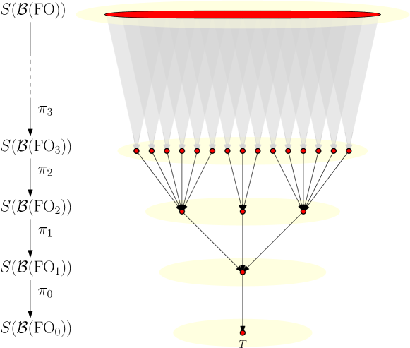
Figure 2.2. Ultrafilters projecting to an $\omega$-categorical theory

A theory $T$ is said to have quantifier elimination if, for every $p$ and every formula $\phi\in{\rm FO}_{p}(\lambda)$ there exists $\widetilde{\phi}\in{\rm QF}_{p}(\lambda)$ such that $T\models\phi\leftrightarrow\widetilde{\phi}$. If a theory (in the language of relational structures with given finite signature, like the language of graphs) has quantifier elimination then it is $\omega$-categorical. Indeed, for every $p$, there exists only finitely many quantifier free formulas with $p$ free variables hence (up to equivalence modulo $T$) only finitely many formulas with $p$ free variables. The unique countable model of a complete theory $T$ (in the language of relational structures with given finite signature) with quantifier elimination is ultra-homogeneous, what means that every partial isomorphism of finite induced substructures extends as a full automorphism. In the context of relational structures with given finite signature, the property of having a countable ultra-homogeneous model is equivalent to the property of having quantifier elimination. We provide a proof of this folklore result in the context of graphs in order to illustrate these notions.

Lemma 2.27.

Let $T$ be a complete theory of graphs with no finite model.

Then $T$ has quantifier elimination if and only if some (equivalently, every) countable model of $T$ is ultra-homogeneous.

Proof.

Assume that $T$ has an ultra-homogeneous countable model $G$. Let $(a_{1},\dots,a_{p})$, $(b_{1},\dots,b_{p})$ be $p$-tuples of vertices of $G$. Assume that $a_{i}\mapsto b_{i}$ is an isomorphism between $G[a_{1},\dots,a_{p}]$ and $G[b_{1},\dots,b_{p}]$. Then, as $G$ is ultra-homogeneous, there exists an automorphism $f$ of $G$ such that $f(a_{i})=b_{i}$ for every $1\leq i\leq p$. As the satisfaction of a first-order formula is invariant under the action of the automorphism group, for every formula $\phi\in{\rm FO}_{p}$ the following equivalence holds:

$$G\models\phi(a_{1},\dots,a_{p})\quad\iff\quad G\models\phi(b_{1},\dots,b_{p}).$$

Consider a maximal set $\mathcal{F}$ of $p$-tuples $(v_{1},\dots,v_{p})$ of $G$ such that $G\models\phi(v_{1},\dots,v_{p})$ and no two $p$-tuples induce isomorphic (ordered) induced subgraphs. Obviously $|\mathcal{F}|=2^{O(p^{2})}$ is finite. Moreover, each $p$-tuple $\vec{v}=(v_{1},\dots,v_{p})$ defines a quantifier free formula $\eta_{\vec{v}}$ with $p$ free variables such that $G\models\eta_{\vec{v}}(x_{1},\dots,x_{p})$ if and only if $x_{i}\mapsto v_{i}$ is an isomorphism between $G[x_{1},\dots,x_{p}]$ and $G[v_{1},\dots,v_{p}]$. Hence the following property holds:

$$G\models\phi\leftrightarrow\bigvee_{\vec{v}\in\mathcal{F}}\eta_{\vec{v}}.$$

In other words, $\phi$ is equivalent (modulo $T$) to the quantifier free formula $\widetilde{\phi}=\bigvee_{\vec{v}\in\mathcal{F}}\eta_{\vec{v}}$, that is: $T$ has quantifier elimination.

Conversely, assume that $T$ has quantifier elimination. As notice above, $T$ is $\omega$-categorical thus has a unique countable model. Assume $(a_{1},\dots,a_{p})$ and $(b_{1},\dots,b_{p})$ are $p$-tuples of vertices such that $f:a_{i}\mapsto b_{i}$ is a partial isomorphism. Assume that $f$ does not extend into an automorphism of $G$. Let $(a_{1},\dots,a_{q})$ be a tuple of vertices of $G$ of maximal length such that there exists $b_{p+1},\dots,b_{q}$ such that $a_{i}\mapsto b_{i}$ is a partial isomorphism. Let $a_{q+1}$ be a vertex distinct from $a_{1},\dots,a_{q}$. Let $\phi(x_{1},\dots,x_{q})$ be the formula

$$\begin{split}\bigwedge_{a_{i}\sim a_{j}}(x_{i}\sim x_{j})\wedge\bigwedge_{\neg(a_{i}\sim a_{j})}\neg(x_{i}\sim x_{j})\wedge\bigwedge_{1\leq i\leq q}\neg(x_{i}=x_{j})\\ \quad\wedge\ (\exists y)\ \biggl{(}\bigwedge_{a_{i}\sim a_{q+1}}(x_{i}\sim y)\wedge\bigwedge_{\neg(a_{i}\sim a_{q+1})}\neg(x_{i}\sim y)\wedge\bigwedge_{1\leq i\leq q}\neg(x_{i}=y)\biggr{)}\end{split}$$

As $T$ has quantifier elimination, there exists a quantifier free formula $\widetilde{\phi}$ such that $T\models\phi\leftrightarrow\widetilde{\phi}$. As $G\models\phi(a_{1},\dots,a_{q})$ (witnessed by $a_{q+1}$) it holds that $G\models\widetilde{\phi}(a_{1},\dots,a_{q})$ hence $G\models\widetilde{\phi}(b_{1},\dots,b_{q})$ (as $a_{i}\mapsto b_{i},1\leq i\leq q$ is a partial isomorphism) thus $G\models\phi(b_{1},\dots,b_{q})$. It follows that there exists $b_{q+1}$ such that $a_{i}\mapsto b_{i},1\leq i\leq q+1$ is a partial isomorphism, contradicting the maximality of $(a_{1},\dots,a_{q})$. ∎

When a sequence of graphs is elementarily convergent to an ultra-homogeneous graph (i.e. to a complete theory with quantifier elimination), we shall prove that ${\rm FO}$-convergence reduces to ${\rm QF}$-convergence. This later mode of convergence is of particular interest as it is equivalent to L-convergence.

Lemma 2.28.

Let $(G_{n})_{n\in\mathbb{N}}$ be sequence of graphs that converges elementarily to some ultra-homogeneous graph $\hat{G}$. Then the following properties are equivalent:

• the sequence $(G_{n})_{n\in\mathbb{N}}$ is ${\rm FO}$-convergent;

• the sequence $(G_{n})_{n\in\mathbb{N}}$ is ${\rm QF}$-convergent;

• the sequence $(G_{n})_{n\in\mathbb{N}}$ is L-convergent.

Proof.

As ${\rm FO}$-convergence implies ${\rm QF}$-convergence we only have to prove the opposite direction. Assume that the sequence $(G_{n})_{n\in\mathbb{N}}$ is ${\rm QF}$-convergent. According to Lemma 2.27, for every formula $\phi\in{\rm FO}_{p}$ there exists a quantifier free formula $\widetilde{\phi}\in{\rm QF}_{p}$ such that $\hat{G}\models\phi\leftrightarrow\widetilde{\phi}$ (i.e. ${\rm Th}(\hat{G})$ has quantifier elimination). As $\hat{G}$ is an elementary limit of the sequence $(G_{n})_{n\in\mathbb{N}}$ there exists some $N$ such that for every $n\geq N$ it holds that $G_{n}\models\phi\leftrightarrow\widetilde{\phi}$. It follows that for every $n\geq N$ it holds that $\langle\phi,G_{n}\rangle=\langle\widetilde{\phi},G_{n}\rangle$ hence $\lim_{n\rightarrow\infty}\langle\phi,G_{n}\rangle$ exists. Thus the sequence $(G_{n})_{n\in\mathbb{N}}$ is ${\rm FO}$-convergent. ∎

There are not so many countable ultra-homogeneous graphs.

Theorem 2.29 (Lachlan and Woodrow [56]).

Every infinite countable ultrahomogeneous undirected graph is isomorphic to one of the following:

• the disjoint union of $m$ complete graphs of size $n$, where $m,n\leq\omega$ and at least one of $m$ or $n$ is $\omega$, (or the complement of it);

• the generic graph for the class of all countable graphs not containing $K_{n}$ for a given $n\geq 3$ (or the complement of it);

• the Rado graph R (the generic graph for the class of all countable graphs).

Among them, the Rado graph $R$ (also called “the random graph”) is characterized by the extension property: for every finite disjoint subsets of vertices $A$ and $B$ of $R$ there exists a vertex $z$ of $R-A-B$ such that $z$ is adjacent to every vertex in $A$ and to no vertex in $B$. We deduce for instance the following application of Lemma 2.28.

Example 2.30.

It is known [11, 12] that for every fixed $k$, Paley graphs of sufficiently large order satisfy the $k$-extension property hence the sequence of Paley graphs converge elementarily to the Rado graph. Moreover, Paley graphs is a standard example of quasi-random graphs [23], and the sequence of Paley graphs is L-convergent to the $1/2$-graphon. Thus, according to Lemma 2.28, the sequence of Paley graphs is ${\rm FO}$-convergent.

We now relate more precisely the extension property with quantifier elimination.

Definition 2.31.

Let $k\in\mathbb{N}$. A graph $G$ has the $k$-extension property if, for every disjoint subsets of vertices $A,B$ of $G$ with size $k$ there exists a vertex $z$ not in $A\cup B$ that is adjacent to every vertex in $A$ and to no vertex in $B$. In other words, $G$ has the $k$-extension property if $G$ satisfies the sentence $\Upsilon_{k}$ below:

$$\begin{split}(\forall x_{1},\dots,x_{2k})\quad&\biggl{(}\bigwedge_{1\leq i<j\leq 2k}\neg(x_{i}=x_{j})\\ &\qquad\rightarrow\quad(\exists z)\ \bigwedge_{i=1}^{2k}\neg(x_{i}=z)\wedge\bigwedge_{i=1}^{k}(x_{i}\sim z)\wedge\bigwedge_{i=k+1}^{2k}\neg(x_{i}\sim z)\biggr{)}.\end{split}$$

Lemma 2.32.

Let $G$ be a graph and let $p,r$ be integers.

If $G$ has the $(p+r)$-extension property then every formula $\phi$ with $p$ free variables and quantifier rank $r$ is equivalent, in $G$, with a quantifier free formula.

Proof.

Let $\phi$ be a formula with $p$ free variables and quantifier rank $r$. Let $(a_{1},\dots,a_{p})$ and $(b_{1},\dots,b_{p})$ be two $p$-tuples of vertices of $G$ such that $a_{i}\mapsto b_{i}$ is a partial isomorphism. The $(p+r)$-extension properties allows to easily play a $r$-turns back-and-forth game between $(G,a_{1},\dots,a_{p})$ and $(G,b_{1},\dots,b_{p})$, thus proving that $(G,a_{1},\dots,a_{p})$ and $(G,b_{1},\dots,b_{p})$ are $r$-equivalent. It follows that $G\models\phi(a_{1},\dots,a_{p})$ if and only if $G\models\phi(b_{1},\dots,b_{p})$. Following the lines of Lemma 2.27, we deduce that there exists a quantifier free formula $\widetilde{\phi}$ such that $G\models\phi\leftrightarrow\widetilde{\phi}$. ∎

We now prove that random graphs converge elementarily to the countable random graphs.

Lemma 2.33.

Let $1/2>\delta>0$. Assume that for every positive integer $n\geq 2$ and every $1\leq i<j\leq n$, $p_{n,i,j}\in[\delta,1-\delta]$. Assume that for each $n\in\mathbb{N}$, $G_{n}$ is a random graph on $[f(n)]$ where $f(n)\geq n$, and where $i$ and $j$ are adjacent with probability $p_{n,i,j}$ (all these events being independent). Then the sequence $(G_{n})_{n\in\mathbb{N}}$ almost surely converges elementarily to the Rado graph.

Proof.

Let $p\in\mathbb{N}$ and let $\alpha=\delta(1-\delta)$. The probability that $G_{n}\models\Upsilon_{p}$ is at least $1-(1-\alpha^{p})^{f(n)}$. It follows that for $N\in\mathbb{N}$ the probability that all the graphs $G_{n}$ ($n\geq N$) satisfy $\Upsilon_{p}$ is at least $1-\alpha^{-p}(1-\alpha^{p})^{f(N)}$. According to Borel-Cantelli lemma, the probability that $G_{n}$ does not satisfy $\Upsilon_{p}$ infinitely many is zero. As this holds for every integer $p$, it follows that, with high probability, every elementarily converging subsequence of $(G_{n})_{n\in\mathbb{N}}$ converges to the Rado graph hence, with high probability, $(G_{n})_{n\in\mathbb{N}}$ converges elementarily to the Rado graph. ∎

Thus we get:

Theorem 2.34.

Let $0<p<1$ and let $G_{n}\in G(n,p)$ be independent random graphs with edge probability $p$. Then $(G_{n})_{n\in\mathbb{N}}$ is almost surely ${\rm FO}$-convergent.

Proof.

This is an immediate consequence of Lemma 2.28, Lemma 2.33 and the easy fact that $(G_{n})_{n\in\mathbb{N}}$ is almost surely ${\rm QF}$-convergent. ∎

Theorem 2.35.

For every $\phi\in{\rm FO}_{p}$ there exists a polynomial $P_{\phi}\in\mathbb{Z}[X_{1},\dots,X_{\binom{p}{2}}]$ such that for every sequence $(G_{n})_{n\in\mathbb{N}}$ of finite graphs that converges elementarily to the Rado graph the following holds:

If $(G_{n})_{n\in\mathbb{N}}$ is L-convergent to some graphon $W$ then

$$\lim_{n\rightarrow\infty}\langle\phi,G_{n}\rangle=\idotsint P_{\phi}((W_{i,j}(x_{i},x_{j}))_{1\leq i<j\leq p})\,{\rm d}x_{1}\dots\rm dx_{p}.$$

Proof.

Assume the sequence $(G_{n})_{n\in\mathbb{N}}$ is elementarily convergent to the Rado graph and that it is L-convergent to some graphon $W$.

According to Lemma 2.27, there exists a quantifier free formula $\widetilde{\phi}$ such that

$$G\models(\forall x_{1}\dots x_{p})\ \phi(x_{1},\dots,x_{p})\leftrightarrow\widetilde{\phi}(x_{1},\dots,x_{p})$$

(hence $\Omega_{\phi}(G)=\Omega_{\widetilde{\phi}}(G)$) holds when $G$ is the Rado graph. As $(G_{n})_{n\in\mathbb{N}}$ is elementarily convergent to the Rado graph, this sentence holds for all but finitely many graphs $G_{n}$. Thus for all but finitely many $G_{n}$ it holds that $\langle\phi,G_{n}\rangle=\langle\widetilde{\phi},G_{n}\rangle$. Moreover, according to Lemma 2.28, the sequence $(G_{n})_{n\in\mathbb{N}}$ is ${\rm FO}$-convergent and thus the following equation holds:

$$\lim_{n\rightarrow\infty}\langle\phi,G_{n}\rangle=\lim_{n\rightarrow\infty}\langle\widetilde{\phi},G_{n}\rangle.$$

By using an inclusion/exclusion argument and the general form of the density of homomorphisms of fixed target graphs to a graphon we deduce that there exists a polynomial $P_{\phi}\in\mathbb{Z}[X_{1},\dots,X_{\binom{p}{2}}]$ (which depends only on $\phi$) such that

$$\lim_{n\rightarrow\infty}\langle\widetilde{\phi},G_{n}\rangle=\idotsint P_{\phi}((W_{i,j}(x_{i},x_{j}))_{1\leq i<j\leq p})\,{\rm d}x_{1}\dots\rm dx_{p}.$$

The theorem follows. ∎

Although elementary convergence to Rado graph seems quite a natural assumption for graphs which are neither too sparse nor too dense, elementary convergence to other ultra-homogeneous graphs may be problematic.

Example 2.36.

Cherlin [21] posed the problem whether there is a finite $k$-saturated triangle-free graph, for each $k\in\mathbb{N}$, where a triangle free graph is called $k$-saturated if for every set $S$ of at most $k$ vertices, and for every independent subset $T$ of $S$, there exists a vertex adjacent to each vertex of $T$ and to no vertex of $S-T$. In other words, Cherlin asks whether the generic countable triangle-free graph has the finite model property, that is if it is an elementary limit of a sequence of finite graphs. See [50] for more ultra-homogeneous structures defined by forbidden substructures.

It is possible to extend Lemma 2.28 to sequences of graph having a non ultra-homogeneous elementary limit if we restrict ${\rm FO}$ to a smaller fragment. An example is the following:

Example 2.37.

A graph $G$ is IH-Homogeneous [18] if every partial finite isomorphism extends into an endomorphism. Let ${\rm PP}$ be the fragment of ${\rm FO}$ that consists into primitive positive formulas, that is formulas formed using adjacency, equality, conjunctions and existential quantification only, and let ${\rm BA}({\rm PP})$ be the minimum sub-Boolean algebra of ${\rm FO}$ containing ${\rm PP}$.

Following the lines of Lemma 2.28 and using Theorem 2.14 and Proposition 2.13, one proves that if a sequence of graphs $(G_{n})_{n\in\mathbb{N}}$ converges elementarily to some IH-homogeneous infinite countable graph then $(G_{n})_{n\in\mathbb{N}}$ is ${\rm BA}({\rm PP})$-convergent if and only if it is ${\rm QF}$-convergent.

2.3.5. ${\rm FO}$-convergence of Graphs with Bounded Maximum Degree

We now consider how full ${\rm FO}$-convergence differs to BS-convergence for sequence of graphs with maximum degree at most $D$. As a corollary of Theorems 2.23 and 2.16 we have:

Corollary 2.38.

A sequence $(G_{n})$ of finite graphs with maximum degree at most $d$ such that $\lim_{n\rightarrow\infty}|G_{n}|=\infty$ is ${\rm FO}$-convergent if and only if it is both BS-convergent and elementarily convergent.

2.4. Interpretation Schemes

In the process of this research we discovered the increasing role played by interpretations. They are described in this section.

2.4.1. Continuous Functions and Interpretations

Let $X$ and $Y$ be fragments of ${\rm FO}(\kappa)$ and ${\rm FO}(\lambda)$, respectively. Let $f:S(\mathcal{B}(X))\rightarrow S(\mathcal{B}(Y))$. A function $f:S(\mathcal{B}(X))\rightarrow S(\mathcal{B}(Y))$ is continuous if and only if the inverse image of an open subset of $S(\mathcal{B}(Y))$ is an open subset of $S(\mathcal{B}(X))$. In the case of Stone spaces (where clopen subsets generates the topology), we can further restrict our attention to clopen subsets: $f$ will be continuous if the inverse image of a clopen subset is a clopen subset. In other words, $f$ is continuous if there exists $f^{*}:\mathcal{B}(Y)\rightarrow\mathcal{B}(X)$, such that for every $\phi\in Y$, the following equation holds:

$$f^{-1}(K(\phi))=K(f^{*}(\phi)).$$

It follows that if $f$ is continuous then for every $X$-convergent sequence $(\mathbf{A}_{n})_{n\in\mathbb{N}}$, the sequence $(f(\mathbf{A}_{n}))_{n\in\mathbb{N}}$ is $Y$-convergent. Note that $f^{*}$ will be a homomorphism from $\mathcal{B}(Y)$ to $\mathcal{B}(X)$, and that the duality between $f$ and $f^{*}$ is nothing more the duality between Stone spaces and Boolean algebras.

The above property can be sometimes restated in terms of definable sets in structures. For a fragment $X$ of ${\rm FO}$ and a relational structure $\mathbf{A}$, a subset $F\subseteq A^{p}$ is $X$-definable if there exists a formula $\phi\in X$ with free variables $x_{1},\dots,x_{p}$ such that

$$F=\Omega_{\phi}(\mathbf{A})=\{(v_{1},\dots,v_{p})\in A^{p}:\ \mathbf{A}\models\phi(v_{1},\dots,v_{p})\}.$$

Let $\mathbf{A}$ be a $\kappa$-structure, let $\mathbf{B}$ be a $\lambda$-structure, and let $g:A^{k}\rightarrow B$ be surjective. Assume that there exists a function $g^{*}:Y\rightarrow X$ such that for every $\phi\in Y$ with free variables $x_{1},\dots,x_{p}$ ($p\geq 0$), and every $v_{i,j}\in A$ ($1\leq i\leq p$, $1\leq j\leq k$) the following holds:

$$\mathbf{B}\models\phi(g(v_{1,1},\dots,v_{1,k}),\dots,g(v_{p,1},\dots,v_{p,k}))$$

$$\iff$$

$$\mathbf{A}\models g^{*}(\phi)(v_{1,1},\dots,v_{1,k},\dots,v_{p,1},\dots,v_{p,k})$$

then $g^{*}$ is a homomorphism, and thus it defines a continuous function from $S(\mathcal{B}(X))$ to $S(\mathcal{B}(Y))$. Note that the above formula can be restated as

$$\Omega_{g^{*}(\phi)}(\mathbf{A})=\hat{g}^{-1}(\Omega_{\phi}(\mathbf{B})),$$

where

$$\hat{g}((v_{1,1},\dots,v_{p,k}))=(g(v_{1,1},\dots,v_{1,k}),\dots,g(v_{p,1},\dots,v_{p,k})).$$

In other words, the inverse image of a $Y$-definable set of $\mathbf{B}$ is an $X$-definable set of $\mathbf{A}$.

When $X={\rm FO}(\kappa)$ and $Y={\rm FO}(\lambda)$, the property that the inverse image of a first-order definable set of $\mathbf{B}$ is a first-order definable set of $\mathbf{A}$ leads to the model theoretical notion of interpretation (without parameters) of $\mathbf{B}$ in $\mathbf{A}$. We recall now the formal definition of an interpretation.

Definition 2.39 (Interpretation).

An interpretation of $\mathbf{B}$ in $\mathbf{A}$ with parameters (or without parameters, respectively) with exponent $k$ is a surjective map from a subset of $A^{k}$ onto $B$ such that the inverse image of every set $X$ definable in $\mathbf{B}$ by a first-order formula without parameters is definable in $\mathbf{A}$ by a first-order formula with parameters (or without parameters, respectively).

2.4.2. Interpretation Schemes

The main drawback of interpretations is that they only concerns two specific structures $\mathbf{A}$ and $\mathbf{B}$. However, it is frequent that interpretations naturally generalize to a family of interpretations of $\lambda$-structures in $\kappa$-structures with the same associated homomorphism of Boolean algebras. Moreover, this homomorphism is uniquely defined by the way it transforms each relation in $\lambda$ (including equality) into a formula in $\kappa$ and by the formula which defines the domain of the $\kappa$-structures. This can be formalized as follows.

Definition 2.40 (Interpretation Scheme).

Let $\kappa,\lambda$ be signatures, where $\lambda$ has $q$ relational symbols $R_{1},\dots,R_{q}$ with respective arities $r_{1},\dots,r_{q}$.

An interpretation scheme ${\mathsf{I}}$ of $\lambda$-structures in $\kappa$-structures is defined by an integer $k$ — the exponent of the interpretation scheme — a formula $E\in{\rm FO}_{2k}(\kappa)$, a formula $\theta_{0}\in{\rm FO}_{k}(\kappa)$, and a formula $\theta_{i}\in{\rm FO}_{r_{i}k}(\kappa)$ for each symbol $R_{i}\in\lambda$, such that:

• the formula $E$ defines an equivalence relation of $k$-tuples;

• each formula $\theta_{i}$ is compatible with $E$, in the sense that for every $0\leq i\leq q$ the following property holds:

  $$\bigwedge_{1\leq j\leq r_{i}}\,E(\mathbf{x}_{j},\mathbf{y}_{j})\quad\vdash\quad\theta_{i}(\mathbf{x}_{1},\dots,\mathbf{x}_{r_{i}})\leftrightarrow\theta_{i}(\mathbf{y}_{1},\dots,\mathbf{y}_{r_{i}}),$$

  where $r_{0}=1$, boldface $\mathbf{x}_{j}$ and $\mathbf{y}_{j}$ represent $k$-tuples of free variables, and where $\theta_{i}(\mathbf{x}_{1},\dots,\mathbf{x}_{r_{i}})$ stands for $\theta_{i}(x_{1,1},\dots,x_{1,k},\dots,x_{r_{i},1},\dots,x_{r_{i},k})$.

For a $\kappa$-structure $\mathbf{A}$, we denote by $\mathsf{I}(\mathbf{A})$ the $\lambda$-structure $\mathbf{B}$ defined as follows:

• the domain $B$ of $\mathbf{B}$ is the subset of the $E$-equivalence classes $[\mathbf{x}]\subseteq A^{k}$ of the tuples $\mathbf{x}=(x_{1},\dots,x_{k})$ such that $\mathbf{A}\models\theta_{0}(\mathbf{x})$;

• for each $1\leq i\leq q$ and every $\mathbf{v}_{1},\dots,\mathbf{v}_{s_{i}}\in A^{kr_{i}}$ such that $\mathbf{A}\models\theta_{0}(\mathbf{v}_{j})$ (for every $1\leq j\leq r_{i}$) the following equivalence holds:

  $$\mathbf{B}\models R_{i}([\mathbf{v}_{1}],\dots,[\mathbf{v}_{r_{i}}])\quad\iff\quad\mathbf{A}\models\theta_{i}(\mathbf{v}_{1},\dots,\mathbf{v}_{r_{i}}).$$

From the standard properties of model theoretical interpretations (see, for instance [57] p. 180), we state the following: if $\mathsf{I}$ is an interpretation of $\lambda$-structures in $\kappa$-structures, then there exists a mapping $\tilde{\mathsf{I}}:{\rm FO}(\lambda)\rightarrow{\rm FO}(\kappa)$ (defined by means of the formulas $E,\theta_{0},\dots,\theta_{q}$ above) such that for every $\phi\in{\rm FO}_{p}(\lambda)$, and every $\kappa$-structure $\mathbf{A}$, the following property holds (while letting $\mathbf{B}=\mathsf{I}(\mathbf{A})$ and identifying elements of $B$ with the corresponding equivalence classes of $A^{k}$):

For every $[\mathbf{v}_{1}],\dots,[\mathbf{v}_{p}]\in B^{p}$ (where $\mathbf{v}_{i}=(v_{i,1},\dots,v_{i,k})\in A^{k}$) the following equivalence holds:

$$\mathbf{B}\models\phi([\mathbf{v}_{1}],\dots,[\mathbf{v}_{p}])\quad\iff\quad\mathbf{A}\models\tilde{\mathsf{I}}(\phi)(\mathbf{v}_{1},\dots,\mathbf{v}_{p}).$$

It directly follows from the existence of the mapping $\tilde{\mathsf{I}}$ that an interpretation scheme ${\mathsf{I}}$ of $\lambda$-structures in $\kappa$-structures defines a continuous mapping from $S(\mathcal{B}({\rm FO}(\kappa)))$ to $S(\mathcal{B}({\rm FO}(\lambda)))$. Thus, interpretation schemes have the following general property:

Proposition 2.41.

Let $\mathsf{I}$ be an interpretation scheme of $\lambda$-structures in $\kappa$-structures.

Then, if a sequence $(\mathbf{A}_{n})_{n\in\mathbb{N}}$ of finite $\kappa$-structures is ${\rm FO}$-convergent then the sequence $(\mathsf{I}(\mathbf{A}_{n}))_{n\in\mathbb{N}}$ of (finite) $\lambda$-structures is ${\rm FO}$-convergent.

We shall be mostly interested in very specific and simple types of interpretation schemes.

Definition 2.42.

Let $\kappa,\lambda$ be signatures. A basic interpretation scheme ${\mathsf{I}}$ of $\lambda$-structures in $\kappa$-structures with exponent $k$ is defined by a formula $\theta_{i}\in{\rm FO}_{kr_{i}}(\kappa)$ for each symbol $R_{i}\in\lambda$ with arity $r_{i}$.

For a $\kappa$-structure $\mathbf{A}$, we denote by $\mathsf{I}(\mathbf{A})$ the structure with domain $A^{k}$ such that, for every $R_{i}\in\lambda$ with arity $r_{i}$ and every $\mathbf{v}_{1},\dots,\mathbf{v}_{r_{i}}\in A^{k}$ the following equivalence holds:

$$\mathsf{I}(\mathbf{A})\models R_{i}(\mathbf{v}_{1},\dots,\mathbf{v}_{r_{i}})\quad\iff\quad\mathbf{A}\models\theta_{i}(\mathbf{v}_{1},\dots,\mathbf{v}_{r_{i}}).$$

It is immediate that every basic interpretation scheme $\mathsf{I}$ defines a mapping $\tilde{\mathsf{I}}:{\rm FO}(\lambda)\rightarrow{\rm FO}(\kappa)$ such that for every $\kappa$-structure $\mathbf{A}$, every $\phi\in{\rm FO}_{p}(\lambda)$, and every $\mathbf{v}_{1},\dots,\mathbf{v}_{p}\in A^{k}$ the following equivalence holds:

$$\mathsf{I}(\mathbf{A})\models\phi(\mathbf{v}_{1},\dots,\mathbf{v}_{p})\quad\iff\quad\mathbf{A}\models\tilde{\mathsf{I}}(\phi)(\mathbf{v}_{1},\dots,\mathbf{v}_{p})$$

and

$${\rm qrank}(\tilde{\mathsf{I}}(\phi))\leq k({\rm qrank}(\phi)+\max_{i}{\rm qrank}(\theta_{i})).$$

It follows that for every $\kappa$-structure $\mathbf{A}$, every $\phi\in{\rm FO}_{p}(\lambda)$, the following equation holds:

$$\Omega_{\phi}(\mathsf{I}(\mathbf{A}))=\Omega_{\tilde{\mathsf{I}}(\phi)}(\mathbf{A}).$$

In particular, if $\mathbf{A}$ is a finite structure, the following equation holds:

$$\langle\phi,\mathsf{I}(\mathbf{A})\rangle=\langle\tilde{\mathsf{I}}(\phi),\mathbf{A}\rangle.$$

Chapter 3 Modelings for Sparse Structures

3.1. Relational Samples Spaces

The notion of relational sample space is a strenghtening of the one of relational structure, where it is required that the domain shall be endowed with a suitable structure of a (nice) measurable space.

3.1.1. Definition and Basic Properties

Definition 3.1.

Let $\lambda$ be a signature. A $\lambda$-relational sample space is a $\lambda$-structure $\mathbf{A}$, whose domain $A$ is a standard Borel space with the property that every first-order definable subset of $A^{p}$ is measurable. Precisely, for every integer $p$, and every $\phi\in{\rm FO}_{p}(\lambda)$, denoting

$$\Omega_{\phi}(\mathbf{A})=\{(v_{1},\dots,v_{p})\in A^{p}:\ \mathbf{A}\models\phi(v_{1},\dots,v_{p})\},$$

it holds that $\Omega_{\phi}(\mathbf{A})\in\Sigma_{\mathbf{A}}^{p}$, where $\Sigma_{\mathbf{A}}$ is the Borel $\sigma$-algebra of $A$.

Note, that in the case of graphs, every relational sample space is a Borel graph (that is a graph whose vertex set is a standard Borel space and whose edge set is Borel), but the converse is not true.

Lemma 3.2.

Let $\lambda$ be a signature, let $\mathbf{A}$ be a $\lambda$-structure, whose domain $A$ is a standard Borel space with $\sigma$-algebra $\Sigma_{\mathbf{A}}$.

Then the following conditions are equivalent:

1. $\mathbf{A}$ is a $\lambda$-relational sample space;

2. for every integer $p\geq 0$ and every $\phi\in{\rm FO}_{p}(\lambda)$, it holds that $\Omega_{\phi}(\mathbf{A})\in\Sigma_{\mathbf{A}}^{p}$;

3. for every integer $p\geq 1$ and every $\phi\in{\rm FO}_{p}^{\rm local}(\lambda)$, it holds that $\Omega_{\phi}(\mathbf{A})\in\Sigma_{\mathbf{A}}^{p}$;

4. for all integers $p,q\geq 0$, every $\phi\in{\rm FO}_{p+q}(\lambda)$, and every $a_{1},\dots,a_{q}\in A^{q}$ the set

   $$\{(v_{1},\dots,v_{p})\in A^{p}:\ \mathbf{A}\models\phi(a_{1},\dots,a_{q},v_{1},\dots,v_{p})\}$$

   belongs to $\Sigma_{\mathbf{A}}^{p}$.

Proof.

Items (a) and (b) are equivalent by definition. Also we obviously have the implications (d) $\Rightarrow$ (b) $\Rightarrow$ (c). That (c) $\Rightarrow$ (b) is a direct consequence of Gaifman locality theorem, and the implication (b) $\Rightarrow$ (d) is a direct consequence of Fubini-Tonelli theorem. ∎

Lemma 3.3.

Let $\mathbf{A}$ be a relational sample space, let $a\in A$, and let $\mathbf{A}_{a}$ be the connected component of $\mathbf{A}$ containing $a$.

Then $\mathbf{A}_{a}$ has a measurable domain and, equipped with the $\sigma$-algebra of the Borel sets of $A$ included in $A_{a}$, it is a relational sample space.

Proof.

Let $\phi\in{\rm FO}_{p}^{\rm local}$ and let

$$X=\{(v_{1},\dots,v_{p})\in A_{a}^{p}:\ \mathbf{A}_{a}\models\phi(v_{1},\dots,v_{p})\}.$$

As $\phi$ is local, there is an integer $D$ such that the satisfaction of $\phi$ only depends on the $D$-neighborhoods of the free variables.

For every integer $n\in\mathbb{N}$, denote by $B(\mathbf{A},a,n)$ the substructure of $\mathbf{A}$ induced by all vertices at distance at most $n$ from $a$. By the locality of $\phi$, for every $v_{1},\dots,v_{p}$ at distance at most $n$ from $a$ the following equivalence holds:

$$\mathbf{A}_{a}\models\phi(v_{1},\dots,v_{p})\quad\iff\quad B(\mathbf{A},a,n+D)\models\phi(v_{1},\dots,v_{p}).$$

However, it is easily checked that there is a local first-order formula $\varphi_{n}\in{\rm FO}_{p+1}^{\rm local}$ such that for every $v_{1},\dots,v_{p}$ the following equivalence holds:

$$B(\mathbf{A},a,n+D)\models\phi(v_{1},\dots,v_{p})\wedge\bigwedge_{i=1}^{p}{\rm dist}(a,v_{i})\leq n\quad\iff\quad\mathbf{A}\models\varphi_{n}(a,v_{1},\dots,v_{p}).$$

By Lemma 3.2, it follows that the set $X_{n}=\{(v_{1},\dots,v_{n})\in A:\ \mathbf{A}\models\varphi_{n}(a,v_{1},\dots,v_{p})\}$ is measurable. As $X=\bigcup_{n\in\mathbb{N}}X_{n}$, we deduce that $X$ is measurable (with respect to $\Sigma_{\mathbf{A}}^{p}$). In particular, $A_{a}$ is a Borel subset of $A$ hence $A_{a}$, equipped with the $\sigma$-algebra $\Sigma_{\mathbf{A}_{a}}$ of the Borel sets of $A$ included in $A_{a}$, is a standard Borel set. Moreover, it is immediate that a subset of $A_{a}^{p}$ belongs to $\Sigma_{\mathbf{A}_{a}}^{p}$ if and only if it belongs to $\Sigma_{\mathbf{A}}^{p}$. Hence, every subset of $A_{a}^{p}$ defined by a local formula is measurable with respect to $\Sigma_{\mathbf{A}_{a}}^{p}$. By Lemma 3.2, it follows that $\mathbf{A}_{a}$ is a relational sample space. ∎

3.1.2. Interpretations of Relational Sample Spaces

An elementary interpretation with parameter amounts to distinguishing a single element, the parameter, by adding a new unary symbol to the signature (e.g. representing a root).

Lemma 3.4.

Let $\mathbf{A}$ be a $\lambda$-relational sample space, let $\lambda^{+}$ be the signature obtained from $\lambda$ by adding a new unary symbol $M$ and let $\mathbf{A}^{+}$ be obtained from $\mathbf{A}$ by marking a single $a\in A$ (i.e. $a$ is the only element $x$ of $A^{+}=A$ such that $\mathbf{A}^{+}\models M(x)$).

Then $\mathbf{A}^{+}$ is a relational sample space.

Proof.

Let $\phi\in{\rm FO}_{p}(\lambda^{+})$. There exists $\phi^{\prime}\in{\rm FO}_{p+1}(\lambda)$ such that for every $x_{1},\dots,x_{p}\in A$ the following equivalence holds:

$$\mathbf{A}^{+}\models\phi(x_{1},\dots,x_{p})\quad\iff\quad\mathbf{A}\models\phi(a,x_{1},\dots,x_{p}).$$

According to Lemma 3.2, the set of all $(x_{1},\dots,x_{p})$ such that $\mathbf{A}\models\phi(a,x_{1},\dots,x_{p})$ is measurable. It follows that $\mathbf{A}^{+}$ is a relational sample space. ∎

Lemma 3.5.

Every injective first-order interpretation (with or without parameters) of a relational sample space is a relational sample space.

Precisely, if $f$ is an injective first-order interpretation of a $\lambda$-structure $\mathbf{B}$ in a $\kappa$-relational sample space $\mathbf{A}$ and if we define

$$\Sigma_{\mathbf{B}}=\{X\subseteq B:f^{-1}(X)\in\Sigma_{\mathbf{A}}^{k}\},$$

then $(\mathbf{B},\Sigma_{\mathbf{B}})$ is a relational sample space.

Proof.

According to Lemma 3.4, we can first mark all the parameters and reduce to the case where the interpretation has no parameters.

Let $D$ be the domain of $f$. As $B$ is first-order definable in $\mathbf{B}$, $D$ is first-order definable in $\mathbf{A}$ hence $D\in\Sigma_{\mathbf{A}}^{k}$. Then $D$ is a Borel sub-space of $A^{k}$. As $f$ is a bijection from $D$ to $B$, we deduce that $(B,\Sigma_{\mathbf{B}})$ is a standard Borel space.

Moreover, as the inverse image of every first-order definable set of $\mathbf{B}$ is first-order definable in $\mathbf{A}$, we deduce that $(\mathbf{B},\Sigma_{\mathbf{B}})$ is a $\lambda$-relational sample space. ∎

3.1.3. Disjoint union

Let $\mathbf{H}_{i}$ be $\lambda$-relational sample spaces for $i\in I\subseteq\mathbb{N}$. We define the disjoint union

$${\mathbf{H}}=\coprod_{i\in I}\mathbf{H}_{i}$$

of the $\mathbf{H}_{i}$’s as the relational structure, which is the disjoint union of the $\mathbf{H}_{i}$’s endowed with the $\sigma$-algebra $\Sigma_{\mathbf{H}}=\{\bigcup_{i}X_{i}:\ X_{i}\in\Sigma_{\mathbf{H}_{i}}\}$.

Lemma 3.6.

Let $\mathbf{H}_{i}$ be $\lambda$-relational sample spaces for $i\in I\subseteq\mathbb{N}$. Then $\mathbf{H}=\coprod_{i\in I}\mathbf{H}_{i}$ is a $\lambda$-relational sample space, in which every $H_{i}$ is measurable.

Proof.

We consider the signature $\lambda^{+}$ obtained from $\lambda$ by adding a new binary relation $\varpi$, and the basic interpretation scheme $\mathsf{I}_{1}$ of $\lambda^{+}$-structures in $\lambda$-structures corresponding to the addition of the new relation $\varpi$ by the formula $\theta_{\varpi}=1$. This means that for every $\lambda$-structure $\mathbf{A}$ it holds that $\mathsf{I}_{1}(\mathbf{A})\models(\forall x,y)\ \varpi(x,y)$. Let $\mathbf{H}_{i}^{+}=\mathsf{I}_{1}(\mathbf{H}_{i})$.

Let $\mathbf{H}^{+}=\coprod_{i\in I}\mathbf{H}_{i}^{+}$. Clearly, $\Sigma_{\mathbf{H}^{+}}=\Sigma_{\mathbf{H}}$ and $(H,\Sigma_{\mathbf{H}})$ is a standard Borel space. Moreover, by construction, each $H_{i}$ is measurable.

Let $\phi\in{\rm FO}_{p}(\lambda)$. First notice that for every $(v_{1},\dots,v_{p})\in H^{p+q}$ (which is also $(H^{+})^{p+q}$) it holds that $\Omega_{\phi}(\mathbf{H})=\Omega_{\phi}(\mathbf{H}^{+})$, that is:

$$\mathbf{H}\models\phi(v_{1},\dots,v_{p})\quad\iff\quad\mathbf{H}^{+}\models\phi(v_{1},\dots,v_{p}).$$

It follows from Lemma 2.25 that the set $\Omega_{\phi}(\mathbf{H}^{+})$ may be obtained by Boolean operations, products, and coordinate permutations from sets defined by $\varpi$-local formulas (which we introduced in Section 2.3.3). As all these operations preserve measurability, we can assume that $\phi$ is $\varpi$-local. Then $\Omega_{\phi}(\mathbf{H}^{+})$ is the union of the sets $\Omega_{\phi}(\mathbf{H}_{i})$. All these sets are measurable (as $\mathbf{H}_{i}$ is a modeling) thus their union is measurable (by construction of $\Sigma_{\mathbf{H}}$). It follows that $\mathbf{H}^{+}$ is a relational sample space, and so is $\mathbf{H}$ (every first-order definable set of $\mathbf{H}$ is first-order definable in $\mathbf{H}^{+}$). ∎

3.2. Modelings

We introduced a notion of limit objects — called modelings — for sequences of sparse graphs and structures, which is a natural generalization of graphings. These limit objects are defined by considering a probability measure on a relational sample space. In this section, we show that the most we can expect is that modelings are limit objects for sequence of sparse structures, and we conjecture that an unavoidable qualitative jump occurs for notions of limit structures, which coincides with the nowhere dense/somewhere dense frontier (see Conjecture 1.1).

3.2.1. Definition and Basic Properties

Recall Definitions 1.4 and 1.6: a $\lambda$-modeling $\mathbf{A}$ is a $\lambda$-relational sample space equipped with a probability measure (denoted $\nu_{\mathbf{A}}$), and the Stone pairing of $\phi\in{\rm FO}(\lambda)$ and a $\lambda$-modeling $\mathbf{A}$ is $\langle\phi,\mathbf{A}\rangle=\nu_{\mathbf{A}}^{p}(\Omega_{\phi}(\mathbf{A}))$. Notice that it follows (by Fubini’s theorem) that it holds that

$$\langle\phi,\mathbf{A}\rangle =\int_{\mathbf{x}\in A^{p}}1_{\Omega_{\phi}(\mathbf{A})}(\mathbf{x})\,{\rm d}\nu_{\mathbf{A}}^{p}(\mathbf{x})$$

$$=\idotsint\mathbf{1}_{\Omega_{\phi}(\mathbf{A})}(x_{1},\dots,x_{p})\ {\rm d}\nu_{\mathbf{A}}(x_{1})\,\dots\,{\rm d}\nu_{\mathbf{A}}(x_{p}).$$

Then, generalizing Definition 1.7, we extend the notion of $X$-convergence to modelings:

Definition 3.7 (modeling $X$-limit).

Let $X$ be a fragment of ${\rm FO}(\lambda)$.

If an $X$-convergent sequence $(\mathbf{A}_{n})_{n\in\mathbb{N}}$ of $\lambda$-modelings satisfies

$$(\forall\phi\in X)\quad\langle\phi,\mathbf{L}\rangle=\lim_{n\rightarrow\infty}\langle\phi,\mathbf{A}_{n}\rangle$$

for some $\lambda$-modeling $\mathbf{L}$, then we say that $\mathbf{L}$ is a modeling $X$-limit of $(\mathbf{A}_{n})_{n\in\mathbb{N}}$.

A $\lambda$-modeling $\mathbf{A}$ is weakly uniform if all the singletons of $A$ have the same measure. Clearly, every finite $\lambda$-structure $\mathbf{A}$ can be identified with the weakly uniform modeling obtained by considering the discrete topology on $A$. This identification is clearly consistent with our definition of the Stone pairing of a formula and a modeling.

In the case where a modeling $\mathbf{A}$ has an infinite domain, the condition for $\mathbf{A}$ to be weakly uniform is equivalent to the condition for $\nu_{\mathbf{A}}$ to be atomless. This property is usually fulfilled by modeling $X$-limits of sequences of finite structures.

Lemma 3.8.

Let $X$ be a fragment of ${\rm FO}$ that includes ${\rm FO}_{0}$ and the formula $(x_{1}=x_{2})$. Then every modeling $X$-limit of weakly uniform modelings is weakly uniform.

Proof.

Let $\phi$ be the formula $(x_{1}=x_{2})$. Notice that for every finite $\lambda$-structure $\mathbf{A}$ it holds that $\langle\phi,\mathbf{A}\rangle=1/|A|$ and that for every infinite weakly uniform $\lambda$-structure it holds that $\langle\phi,\mathbf{A}\rangle=0$.

Let $\mathbf{L}$ be a modeling $X$-limit of a sequence $(\mathbf{A}_{n})_{n\in\mathbb{N}}$. Assume $\lim_{n\rightarrow\infty}|A_{n}|=\infty$. Assume for contradiction that $\nu_{\mathbf{L}}$ has an atom $\{v\}$ (i.e. $\nu_{\mathbf{L}}(\{v\})>0$). Then $\langle\phi,\mathbf{L}\rangle\geq\nu_{\mathbf{L}}(\{v\})^{2}>0$, contradicting $\lim_{n\rightarrow\infty}\langle\phi,\mathbf{A}_{n}\rangle=0$. Hence $\nu_{\mathbf{L}}$ is atomless.

Otherwise, $|L|=\lim_{n\rightarrow\infty}|A_{n}|<\infty$ (as $\mathbf{L}$ is an elementary limit of $(\mathbf{A}_{n})_{n\in\mathbb{N}}$). Let $N=|L|$. Label $v_{1},\dots,v_{N}$ the elements of $L$ and let $p_{i}=\nu_{\mathbf{L}}(\{v_{i}\})$. Then

$$\frac{1}{N}\sum_{i=1}^{N}p_{i}^{2}-\Bigl{(}\frac{1}{N}\sum_{i=1}^{N}p_{i}\Bigr{)}^{2} =\frac{\langle\phi,\mathbf{L}\rangle}{N}-\frac{1}{N^{2}}$$

$$=\frac{\lim_{n\rightarrow\infty}\langle\phi,\mathbf{A}_{n}\rangle}{N}-\frac{1}{N^{2}}$$

$$=0$$

Thus $p_{i}=1/N$ for every $i=1,\dots,N$. ∎

Corollary 3.9.

Every modeling ${\rm FO}_{2}^{\rm local}$-limit of finite structures is weakly uniform.

Lemma 3.10.

Let $X$ be a fragment that includes all quantifier free formulas.

Assume $\mathbf{L}$ is a modeling $X$-limit of a sequence $(G_{n})_{n\in\mathbb{N}}$ of graphs with $|G_{n}|\rightarrow\infty$. Let $\overline{\nu}_{\mathbf{L}}$ be the completion of the measure $\nu_{\mathbf{L}}$.

Then there is at least one mod $0$ isomorphism $f:[0,1]\rightarrow(L,\overline{\nu}_{\mathbf{L}})$, and for every such $f$ the graphon $W$ defined by

$$W(x,y)=\mathbf{1}_{\Omega_{(x_{1}\sim x_{2})}(\mathbf{L})}(f(x),f(y))$$

(for $x,y$ in the domain of $f$, and $W(x,y)=0$ elsewhere) is a random-free graphon L-limit of $(G_{n})_{n\in\mathbb{N}}$.

Proof.

Considering the formula $x_{1}=x_{2}$, we infer that $\nu_{\mathbf{L}}$ is atomless. This measure is also atomless and turns $L$ into a standard probability space. According to the isomorphism theorem, all atomless standard probability spaces are mutually mod $0$ isomorphic hence there is at least one mod $0$ isomorphism $f:[0,1]\rightarrow(L,\overline{\nu}_{\mathbf{L}})$ ($[0,1]$ is considered with Lebesgue measure).

Fix such a mod $0$ isomorphism $f$, defined on $[0,1]\setminus N_{1}$, with value on $L\setminus N_{2}$ (where $N_{1}$ and $N_{2}$ are nullsets). For every Borel measurable function $g:L^{n}\rightarrow[0,1]$, define $g_{f}$ by $g_{f}(x_{1},\dots,x_{n})=g(f(x_{1}),\dots,f(x_{n}))$ if $x_{i}\notin N_{1}$ for every $1\leq i\leq n$ and $g_{f}(x_{1},\dots,x_{n})=0$ otherwise. Then it holds that

$$\int_{[0,1]^{n}}g_{f}(x_{1},\dots,x_{n})\,{\rm d}x_{1}\dots\rm dx_{n} =\int_{L^{n}}g(v_{1},\dots,v_{n})\,{\rm d}\overline{\nu}_{\mathbf{L}}(v_{1})\dots\rm d\overline{\nu}_{\mathbf{L}}(v_{n})$$

$$=\int_{L^{n}}g(v_{1},\dots,v_{n})\,{\rm d}\nu_{\mathbf{L}}(v_{1})\dots\rm d\nu_{\mathbf{L}}(v_{n}).$$

It follows that for every finite graph $F$ with vertex set $\{1,\dots,n\}$, denoting by $\phi_{F}$ the formula $\bigwedge_{ij\in E(F)}(x_{i}\sim x_{j})$, it holds that

$$t(F,W) =\int_{[0,1]^{n}}\prod_{ij\in E(F)}W(x_{i},x_{j})\,{\rm d}x_{1}\dots\rm dx_{n}$$

$$=\int_{L^{n}}\prod_{ij\in E(F)}\mathbf{1}_{\Omega_{(x_{1}\sim x_{2})}(\mathbf{L})}(v_{i},v_{j})\,{\rm d}\nu_{\mathbf{L}}(v_{1})\dots\rm d\nu_{\mathbf{L}}(v_{n})$$

$$=\int_{L^{n}}\mathbf{1}_{\Omega_{\phi_{F}}(\mathbf{L})}(v_{1},\dots,v_{n})\,{\rm d}\nu_{\mathbf{L}}(v_{1})\dots\rm d\nu_{\mathbf{L}}(v_{n})$$

$$=\langle\phi_{F},\mathbf{L}\rangle$$

$$=\lim_{n\rightarrow\infty}\langle\phi_{F},G_{n}\rangle$$

$$=\lim_{n\rightarrow\infty}t(F,G_{n}).$$

Hence $W$ is a graphon L-limit of $(G_{n})_{n\in\mathbb{N}}$. As $W$ is $\{0,1\}$-valued, it is (by definition) random-free. ∎

We deduce the following limitation of modelings as limit objects.

Corollary 3.11.

Let $X$ be a fragment that includes all quantifier free formulas.

Assume $(G_{n})_{n\in\mathbb{N}}$ is an $X$-convergent sequence of graphs with unbounded order, which is L-convergent to some non random-free graphon $W$. Then $(G_{n})_{n\in\mathbb{N}}$ has no modeling $X$-limit.

Let us now give some example stressing that the nullsets of the mod $0$ isomorphism $f$ can be quite large, making $\mathbf{L}$ and $W$ look quite different. We now give an example in the more general setting of directed graphs and non-symmetric graphons.

Example 3.12.

Let $\vec{T}_{n}$ be the transitive tournament of order $n$, that is the directed graph on $\{1,\dots,n\}$ defined from the natural linear order $<_{n}$ on $\{1,\dots,n\}$ by $i\rightarrow j$ if $i<j$. This sequence is obviously ${\rm FO}$-convergent.

It is not difficult to construct a modeling ${\rm FO}$-limit of $(\vec{T}_{n})_{n\in\mathbb{N}}$: Let

$$L=(\{0\}\times\mathbb{Z}^{+})\cup(\,]0,1[\times\mathbb{Z})\cup(\{1\}\times\mathbb{Z}^{-}),$$

with the Borel $\sigma$-algebra $\Sigma$ generated by the product topology of $\mathbb{Z}$ (with discrete topology) and $\mathbb{R}$ (with usual topology). On $L$ we define a linear order $<_{L}$ by $(\alpha,i)<_{L}(\beta,j)$ if $\alpha<\beta$ or $(\alpha=\beta)$ and $(i<j)$. That $(L,\Sigma)$ is a relational sample space follows from the o-minimality of $([0,1],<)$. The measure $\nu_{\mathbf{L}}$ can be defined as the product of Lebesgue measure on $[0,1]$ by any probability measure on $\mathbb{Z}$. For instance, for every $B\in\Sigma$ we let $\nu_{\mathbf{L}}(B)=\lambda(B\cap([0,1]\times\{0\}))$, where $\lambda$ is Lebesgue measure. It is not difficult to check that $\mathbf{L}$ is indeed a modeling ${\rm FO}$-limit of $(\{1,\dots,n\},<_{n})\simeq\vec{T}_{n}$.

In this case, a mod $0$ isomorphism $f$ defined on $[0,1]$ with values in $L\setminus N_{2}$ (where $N_{2}$ is a nullset) can be defined by $f(x)=(x,0)$. The null set $N_{2}$, although very large, is clearly a $\nu_{\mathbf{L}}$-nullset, and the obtained (non symmetric) random-free graphon $W:[0,1]\times[0,1]\rightarrow[0,1]$ is simply defined by

$$W(x,y)=\begin{cases}1&\text{if }x<y\\ 0&\text{otherwise.}\end{cases}$$

Note that $W$ corresponds to $[0,1]$ with its natural order $<$. This order is clearly an L-limit of $<_{n}$ (but not an elementary limit, as it is dense although no finite order is).

In the spirit of Lemma 3.2, we propose the following problems:

Problem 3.1.

Let $\mathbf{L}$ be a modeling ${\rm FO}$-limit of a sequence $(\mathbf{A}_{n})_{n\in\mathbb{N}}$ of $\lambda$-structures, and let $v\in L$. Does there exist a sequence $(v_{n})_{n\in\mathbb{N}}$ such that $v_{n}\in A_{n}$ and such that the rooted modeling $(\mathbf{L},v)$ is a modeling ${\rm FO}$-limit of the rooted structures $(\mathbf{A}_{n},v_{n})$?

Problem 3.2.

Let $\mathbf{L}$ be a modeling ${\rm FO}$-limit of a sequence $(\mathbf{A}_{n})_{n\in\mathbb{N}}$ of $\lambda$-structures. Does there exist $f:L\rightarrow\prod_{i\in\mathbb{N}}A_{n}$ such that for every $v_{1},\dots,v_{k}\in L$, the $k$-rooted modeling $(\mathbf{L},v_{1},\dots,v_{k})$ is a modeling ${\rm FO}$-limit of the $k$-rooted structures $(\mathbf{A}_{n},f(v_{1})_{n},\dots,f(v_{k})_{n})$?

3.2.2. Interpretation Schemes applied to Modelings

Basic interpretation schemes will be an efficient tool to handle modelings. Let $\mathsf{I}$ be an interpretation scheme ${\mathsf{I}}$ of $\lambda$-structures in $\kappa$-structures. We have seen that $\mathsf{I}$ can be extended to a mapping from $\kappa$-relational sample space to $\lambda$-relational sample space. In the case where $\mathsf{I}$ is a basic interpretation scheme, we further extend $\mathsf{I}$ to a mapping from $\kappa$-modeling to $\lambda$-modeling: For a $\kappa$-modeling $\mathbf{A}$, the $\lambda$-modeling $\mathbf{B}=\mathsf{I}(\mathbf{A})$ is the modeling on the image relational sample space of $\mathbf{A}$ with the probability measure $\nu_{\mathbf{B}}=\nu_{\mathbf{A}}$. This is formalized as follows:

Lemma 3.13.

Let $\mathsf{I}$ be a basic interpretation scheme ${\mathsf{I}}$ of $\lambda$-structures in $\kappa$-structures with exponent $k$. Extend the definition of $\mathsf{I}$ to a mapping of $\kappa$-modeling to $\lambda$-modeling by setting $\nu_{\mathsf{I}(\mathbf{A})}=\nu_{\mathbf{A}}^{k}$. Then for every $\kappa$-modeling $\mathbf{A}$ and every $\phi\in{\rm FO}(\lambda)$ the following equation holds:

$$\langle\phi,\mathsf{I}(\mathbf{A})\rangle=\langle\tilde{\mathsf{I}}(\phi),\mathbf{A}\rangle.$$

Proof.

Let $\mathbf{A}$ be a $\kappa$-modeling. For every $\phi\in{\rm FO}_{p}(\lambda)$ the following equation holds:

$$\Omega_{\phi}(\mathsf{I}(\mathbf{A}))=\Omega_{\tilde{\mathsf{I}}(\phi)}(\mathbf{A})$$

thus $\langle\phi,\mathsf{I}(\mathbf{A})\rangle=\nu_{\mathsf{I}(\mathbf{A})}^{p}(\Omega_{\phi}(\mathsf{I}(\mathbf{A})))=\nu_{\mathbf{A}}^{kp}(\Omega_{\tilde{\mathsf{I}}(\phi)}(\mathbf{A}))=\langle\tilde{\mathsf{I}}(\phi),\mathbf{A}\rangle$. ∎

Remark 3.14.

If the basic interpretation scheme $\mathsf{I}$ is defined by quantifier free formulas only, then it is possible to define $\widetilde{\mathsf{I}}$ in such a way that for every $\phi\in{\rm FO}(\lambda)$ it holds that ${\rm qrank}(\widetilde{\mathsf{I}}(\phi))\leq{\rm qrank}(\phi)$.

The following strengthening of Proposition 2.41 in the case where we consider a basic interpretation scheme is a clear consequence of Lemma 3.13.

Proposition 3.15.

Let $\mathsf{I}$ be a basic interpretation scheme of $\lambda$-structures in $\kappa$-structures.

If $\mathbf{L}$ is a modeling ${\rm FO}$-limit of a sequence $(\mathbf{A}_{n})_{n\in\mathbb{N}}$ of $\kappa$-modelings then $\mathsf{I}(\mathbf{L})$ is a modeling ${\rm FO}$-limit of the sequence $(\mathsf{I}(\mathbf{A}_{n}))_{n\in\mathbb{N}}$.

Remark 3.16.

Let us mention that interpretations can be used to generalize graphings to bounded degree $k$-regular hypergraphs, and even to bounded degree relational structures: Define the degree of an element of a $\lambda$-structure as the number of relations it belongs to. Following the lines of Proposition 3.15 and considering a natural interpretation of $\lambda$-structures with maximum degree $D$ in colored (multi)graphs with maximum degree $\max(D,r)$ (where $r$ is the maximum arity of a relation in $\lambda$) we deduce from Corollary 2.38 that classes of relational structures with bounded maximum degree have modeling FO-limits.

Lemma 3.17.

Let $p\in\mathbb{N}$ be a positive integer, let $\mathbf{L}$ be a modeling, and let $\tensor*[^{p}_{\scriptscriptstyle\mathbf{L}}]{\sf\textstyle Tp}{}:L^{p}\rightarrow S(\mathcal{B}({\rm FO}_{p}(\lambda)))$ be the function mapping $(v_{1},\dots,v_{p})\in L^{p}$ to the complete theory of $(\mathbf{L},v_{1},\dots,v_{p})$ (that is the set of the formulas $\varphi\in{\rm FO}_{p}(\lambda)$ such that $\mathbf{L}\models\varphi(v_{1},\dots,v_{p})$).

Then $\tensor*[^{p}_{\scriptscriptstyle\mathbf{L}}]{\sf\textstyle Tp}{}$ is a measurable map from $(L^{p},\Sigma_{\mathbf{L}}^{p})$ to $S(\mathcal{B}({\rm FO}_{p}(\lambda)))$ (with its Borel $\sigma$-algebra).

Let $(\mathbf{A}_{n})_{n\in\mathbb{N}}$ be an ${\rm FO}_{p}(\lambda)$-convergent sequence of finite $\lambda$-structures, and let $\mu_{p}$ be the associated limit measure (as in Theorem 2.6).

Then $\mathbf{L}$ is an ${\rm FO}_{p}(\lambda)$-limit modeling of $(\mathbf{A}_{n})_{n\in\mathbb{N}}$ if and only if $\mu_{p}$ is the pushforward of the product measure $\nu_{\mathbf{L}}^{p}$ by the measurable map $\tensor*[^{p}_{\scriptscriptstyle\mathbf{L}}]{\sf\textstyle Tp}{}$, that is:

$$\tensor*[^{p}_{\scriptscriptstyle\mathbf{L}}]{\sf\textstyle Tp}{}_{*}(\nu_{\mathbf{L}}^{p})=\mu_{p}.$$

Proof.

Recall that the clopen sets of $S(\mathcal{B}({\rm FO}_{p}(\lambda)))$ are of the form $K(\phi)$ for $\phi\in{\rm FO}_{p}(\lambda)$ and that they generate the topology of $S(\mathcal{B}({\rm FO}_{p}(\lambda)))$ hence also its Borel $\sigma$-algebra.

That $\tensor*[^{p}_{\scriptscriptstyle\mathbf{L}}]{\sf\textstyle Tp}{}$ is measurable follows from the fact that for every $\phi\in{\rm FO}_{p}$ the preimage of $K(\phi)$, that is $\tensor*[^{p}_{\scriptscriptstyle\mathbf{L}}]{\sf\textstyle Tp}{}^{-1}(K(\phi))=\Omega_{\phi}(\mathbf{L})$, is measurable.

Assume that $\mathbf{L}$ is an ${\rm FO}_{p}(\lambda)$-limit modeling of $(\mathbf{A}_{n})_{n\in\mathbb{N}}$. In order to prove that $\tensor*[^{p}_{\scriptscriptstyle\mathbf{L}}]{\sf\textstyle Tp}{}_{*}(\nu_{\mathbf{L}}^{p})=\mu_{p}$, it is sufficient to check it on sets $K(\phi)$:

$$\mu_{p}(K(\phi))=\lim_{n\rightarrow\infty}\langle\phi,\mathbf{A}_{n}\rangle=\langle\phi,\mathbf{L}\rangle=\nu_{\mathbf{L}}^{p}(\tensor*[^{p}_{\scriptscriptstyle\mathbf{L}}]{\sf\textstyle Tp}{}^{-1}(K(\phi))).$$

Conversely, if $\tensor*[^{p}_{\scriptscriptstyle\mathbf{L}}]{\sf\textstyle Tp}{}_{*}(\nu_{\mathbf{L}}^{p})=\mu_{p}$ then for every $\phi\in{\rm FO}_{p}(\lambda)$ the following equation holds:

$$\langle\phi,\mathbf{L}\rangle=\nu_{\mathbf{L}}^{p}(\tensor*[^{p}_{\scriptscriptstyle\mathbf{L}}]{\sf\textstyle Tp}{}^{-1}(K(\phi)))=\mu_{p}(K(\phi))=\lim_{n\rightarrow\infty}\langle\phi,\mathbf{A}_{n}\rangle,$$

hence $\mathbf{L}$ is an ${\rm FO}_{p}(\lambda)$-limit modeling of $(\mathbf{A}_{n})_{n\in\mathbb{N}}$. ∎

If $(X,\Sigma)$ is a Borel space with a probability measure $\nu$, it is standard to define the product $\sigma$-algebra $\Sigma^{\omega}$ on the infinite product space $X^{\mathbb{N}}$, which is generated by cylinder sets of the form

$$R=\{f\in X^{\mathbb{N}}:\ f(i_{1})\in A_{i_{1}},\dots,f(i_{k})\in A_{i_{k}}\}$$

for some $k\in\mathbb{N}$ and $A_{i_{1}},\dots,A_{i_{k}}\in\Sigma$. The measure $\nu^{\omega}$ of the cylinder $R$ defined above is then

$$\nu^{\omega}(R)=\prod_{j=1}^{k}\nu(A_{i_{j}}).$$

By Kolmogorov’s Extension Theorem, this extends to a unique probability measure on $\Sigma^{\omega}$ (which we still denote by $\nu^{\omega}$). We summarize this as the following (see also Fig. 3.1).

Theorem 3.18.

let $\mathbf{L}$ be a modeling, and let $\tensor*[^{\omega}_{\scriptscriptstyle\mathbf{L}}]{\sf\textstyle Tp}{}:L^{\mathbb{N}}\rightarrow S(\mathcal{B}({\rm FO}(\lambda)))$ be the function which assigns to $f\in L^{\mathbb{N}}$ the point of $S(\mathcal{B}({\rm FO}(\lambda)))$ corresponding to the set $\{\phi:\mathbf{L}\models\phi(f(1),\dots,f(p)),\text{ where }{\rm Fv}(\phi)\subseteq\{1,\dots,p\}\}$.

Then $\tensor*[^{\omega}_{\scriptscriptstyle\mathbf{L}}]{\sf\textstyle Tp}{}$ is a measurable map.

Let $(\mathbf{A}_{n})_{n\in\mathbb{N}}$ be an ${\rm FO}(\lambda)$-convergent sequence of finite $\lambda$-structures, and let $\mu$ be the associated limit measure (see Theorem 2.4).

Then $\mathbf{L}$ is an ${\rm FO}(\lambda)$-limit modeling of $(\mathbf{A}_{n})_{n\in\mathbb{N}}$ if and only if

$$\tensor*[^{\omega}_{\scriptscriptstyle\mathbf{L}}]{\sf\textstyle Tp}{}_{*}(\nu_{\mathbf{L}}^{\omega})=\mu.$$

Fig. 3.1 visualizes Lemma 3.17 and Theorem 3.18.

Figure 3.1. Pushforward of measures

Remark 3.19.

We could have considered free variables to be indexed by $\mathbb{Z}$ instead of $\mathbb{N}$. In such a context, natural shift operations $S$ and $T$ act respectively on the Stone space $\mathcal{S}$ of the Lindenbaum–Tarski algebra of ${\rm FO}(\lambda)$, and on the space $\mathbf{L}^{\mathbb{Z}}$ of the mappings from $\mathbb{Z}$ to a $\lambda$-modeling $\mathbf{L}$. If $(\mathbf{A}_{n})_{n\in\mathbb{N}}$ is an ${\rm FO}$-convergent sequence with limit measure $\mu$ on $\mathcal{S}$, then $(\mathcal{S},\mu,S)$ is a measure-preserving dynamical system. Also, if $\nu^{\mathbb{Z}}$ is the product measure on $\mathbf{A}$, $(\mathbf{A}^{\mathbb{Z}},\nu,T)$ is a Bernoulli scheme. Then, the condition of Theorem 3.18 can be restated as follows: the modeling $\mathbf{L}$ is a modeling ${\rm FO}$-limit of the sequence $(\mathbf{A}_{n})_{n\in\mathbb{N}}$ if and only if $(\mathcal{S},\mu,S)$ is a factor of $(\mathbf{A}^{\mathbb{Z}},\nu^{\mathbb{Z}},T)$. This setting leads to yet another interpretation of our result, which we hope will be treated elsewhere.

3.2.3. Component-Local Formulas

The basic observation is that for $\varpi$-local formulas, we can reduce the Stone pairing to components.

Lemma 3.20.

Let $\mathbf{A}$ be a $\lambda$-modeling and component relation $\varpi$. Let $\psi\in{\rm FO}_{p}(\lambda)$ be a $\varpi$-local formula of $\mathbf{A}$.

Assume $\mathbf{A}$ has countably many connected components $\{\mathbf{B}_{i}\}_{i\in\Gamma}$. Let $\Gamma_{+}$ be the set of indexes $i$ such that $\nu_{\mathbf{A}}(B_{i})>0$. For $i\in\Gamma_{+}$ we equip $\mathbf{B}_{i}$ with the $\sigma$-algebra $\Sigma_{\mathbf{B}_{i}}$ and the probability measure $\nu_{\mathbf{B}_{i}}$, where $\Sigma_{\mathbf{B}_{i}}$ is restriction of $\Sigma_{\mathbf{A}}$ to $B_{i}$ and, for $X\in\Sigma_{\mathbf{B}_{i}}$, $\nu_{\mathbf{B}_{i}}(X)=\nu_{\mathbf{A}}(X)/\nu_{\mathbf{A}}(B_{i})$. Then

$$\langle\psi,\mathbf{A}\rangle=\sum_{i\in\Gamma}\nu_{\mathbf{A}}(B_{i})^{p}\,\langle\psi,\mathbf{B}_{i}\rangle.$$

Proof.

First note that each connected component of $\mathbf{A}$ is measurable: let $\mathbf{B}_{i}$ be a connected component of $\mathbf{A}$ and let $a\in B_{i}$. Then $B_{i}=\{x\in A:\mathbf{A}\models\varpi(x,a)\}$ hence $B_{i}$ is measurable as $\mathbf{A}$ is a relational sample space. Let $Y=\{(v_{1},\dots,v_{p})\in A^{p}:\mathbf{A}\models\psi(v_{1},\dots,v_{p})\}$. Then $\langle\psi,\mathbf{A}\rangle=\nu_{\mathbf{A}}^{p}(Y)$. As $\psi$ is $\varpi$-local, it also holds that $Y=\bigcup_{i\in\Gamma}Y_{i}$, where $Y_{i}=\{(v_{1},\dots,v_{p}):\mathbf{B}_{i}\models\psi(v_{1},\dots,v_{p})\}=Y\cap B_{i}^{p}$. As $B_{i}\in\Sigma_{\mathbf{A}}$ and $Y\in\Sigma_{\mathbf{A}}^{p}$, it follows that $Y_{i}\in\Sigma_{\mathbf{A}}^{p}$ and (by countable additivity) it holds that

$$\langle\psi,\mathbf{A}\rangle=\nu_{\mathbf{A}}^{p}(Y)=\sum_{i\in\Gamma}\nu_{\mathbf{A}}^{p}(Y_{i})=\sum_{i\in\Gamma_{+}}\nu_{\mathbf{A}}(\mathbf{B}_{i})^{p}\nu_{\mathbf{B}_{i}}^{p}(Y_{i})=\sum_{i\in\Gamma}\nu_{\mathbf{A}}(\mathbf{B}_{i})^{p}\,\langle\psi,\mathbf{B}_{i}\rangle.$$

∎

Corollary 3.21.

Let $\mathbf{A}$ be a finite $\lambda$-structure with component relation $\varpi$. Let $\psi\in{\rm FO}_{p}(\lambda)$ be a $\varpi$-local formula of $\mathbf{A}$.

Let $\mathbf{B}_{1},\dots,\mathbf{B}_{n}$ be the connected components of $\mathbf{A}$. Then

$$\langle\psi,\mathbf{A}\rangle=\sum_{i=1}^{n}\biggl{(}\frac{|B_{i}|}{|A|}\biggr{)}^{p}\,\langle\psi,\mathbf{B}_{i}\rangle.$$

We are now ready to reduce Stone pairing of local formulas to Stone pairings with $\varpi$-local formulas on connected components.

Theorem 3.22.

Let $p\in\mathbb{N}$ and $\phi\in{\rm FO}_{p}^{\rm local}(\lambda)$.

Then there exist $\varpi$-local formulas $\xi_{i,j}\in{\rm FO}_{q_{i,j}}^{\rm local}$ ($1\leq i\leq n$, $j\in I_{i}$) with ${\rm qrank}(\xi_{i,j})\leq{\rm qrank}(\phi)$ such that for each $i$, $\sum_{j\in I_{i}}q_{i,j}=p$ and, for every modeling $\mathbf{A}$ with component relation $\varpi$ and countable set of connected components $\{\mathbf{B}_{k}\}_{k\in\Gamma}$, the following equation holds:

$$\langle\phi,\mathbf{A}\rangle=\sum_{i=1}^{n}\prod_{j\in I_{i}}\sum_{k\in\Gamma}\nu_{\mathbf{A}}(B_{k})^{q_{i,j}}\langle\xi_{i,j},\mathbf{B}_{k}\rangle.$$

Proof.

This is a direct consequence of Lemmas 2.25 and 3.20. ∎

The case of sentences can be handled easily by limited counting. For a set $X$ and an integer $m$, define

$${\rm Big}_{m}(X)=\begin{cases}1&\text{if }|X|\geq m\\ 0&\text{otherwise}.\end{cases}$$

Lemma 3.23.

Let $\theta\in{\rm FO}_{0}(\lambda)$.

Then there exist formulas $\psi_{1},\dots,\psi_{s}\in{\rm FO}_{1}^{\rm local}$ with quantifier rank at most $q({\rm qrank}(\theta))$, integers $m_{1},\dots,m_{s}\leq{\rm qrank}(\theta)$, and a Boolean function $F$ such that for every $\lambda$-structure $\mathbf{A}$ with component relation $\varpi$ and connected components $\mathbf{B}_{i}$ ($i\in I$), the property $\mathbf{A}\models\theta$ is equivalent to

$$F({\rm Big}_{m_{1}}(\{i,\mathbf{B}_{i}\models(\exists x)\psi_{1}(x)\}),\dots,{\rm Big}_{m_{s}}(\{i,\mathbf{B}_{i}\models(\exists x)\psi_{s}(x)\}))=1.$$

Proof.

Indeed, it follows from the Gaifman locality theorem (Theorem 2.21) that — in the presence of a component relation $\varpi$ — every sentence $\theta$ with quantifier rank $r$ can be written as a Boolean combination of sentences $\theta_{k}$ of the form

$$\exists y_{1}\dots\exists y_{m_{k}}\biggl{(}\bigwedge_{1\leq i<j\leq m_{k}}\neg\varpi(y_{i},y_{j})\wedge\bigwedge_{1\leq i\leq m_{k}}\psi_{k}(y_{i})\biggr{)}$$

where $\psi_{k}$ is $\varpi$-local, $m_{k}\leq{\rm qrank}(\theta)$, and ${\rm qrank}(\psi_{k})\leq q({\rm qrank}(\theta))$, for some fixed function $q$. As $\mathbf{A}\models\theta_{k}$ if and only if ${\rm Big}_{m_{k}}(\{i,\mathbf{B}_{i}\models(\exists x)\psi_{k}(x)\})=1$, the lemma follows. ∎

3.2.4. Convex Combinations of Modelings

In several contexts, it is clear when the disjoint union of converging sequences forms a converging sequence. If two graph sequences $(G_{n})_{n\in\mathbb{N}}$ and $(H_{n})_{n\in\mathbb{N}}$ are L-convergent or BS-convergent, it is clear that the sequence $(G_{n}\cup H_{n})_{n\in\mathbb{N}}$ is also convergent, provided that the limit

$$\lim_{n\rightarrow\infty}|G_{n}|/(|G_{n}|+|H_{n}|)$$

exists. The same applies if we merge a countable set of L-convergent (resp. BS-convergent) sequences $(H_{n,i})_{n\in\mathbb{N}}$ (where $i\in\mathbb{N}$), with the obvious restriction that for each $i\in\mathbb{N}$ all but finitely many $H_{n,i}$ are empty graphs.

We shall see that the possibility of merging a countable set of converging sequences to ${\rm FO}^{\rm local}$-convergence will need a further assumption, namely the following equality:

$$\sum_{i}\lim_{n\rightarrow\infty}\frac{|G_{n,i}|}{|\bigcup_{j}G_{n,j}|}=1.$$

The importance of this assumption is illustrated by the next example.

Example 3.24.

Let $N_{n}=2^{2^{n}}$ (so that $N(n)$ is divisible by $2^{i}$ for every $1\leq i\leq 2^{n}$). Consider sequences $(H_{n,i})_{n\in\mathbb{N}}$ of edgeless black and white colored graphs where $H_{n,i}$ is

• empty if $i>2^{n}$,

• the edgeless graph with $(2^{-i}+2^{-n})N_{n}$ white vertices and $2^{-i}N_{n}$ black vertices if $n$ is odd,

• the edgeless graph with $(2^{-i}+2^{-n})N_{n}$ black vertices and $2^{-i}N_{n}$ white vertices if $n$ is even.

For each $i\in\mathbb{N}$, the sequence $(H_{n,i})_{n\in\mathbb{N}}$ is obviously L-convergent (and even ${\rm FO}$-convergent) as the proportion of white vertices in $H_{n,i}$ tends to $1/2$ as $n\rightarrow\infty$. The order of $G_{n}=\bigcup_{i\in\mathbb{N}}H_{n,i}$ is $3N_{n}$ and $|H_{n,i}|/|G_{n}|$ tends to $\frac{2}{3}\cdot 2^{-i}$ as $n$ goes to infinity. However the sequence $(G_{n})_{n\in\mathbb{N}}$ is not L-convergent (hence not ${\rm FO}^{\rm local}$-convergent). Indeed, the proportion of white vertices in $G_{n}$ is $2/3$ if $n$ is odd and $1/3$ is $n$ is even.

Hence, we are led to the following definition.

Definition 3.25 (Convex combination of Modelings).

Let $\mathbf{H}_{i}$ be $\lambda$-modelings for $i\in I\subseteq\mathbb{N}$ and let $(\alpha_{i})_{i\in I}$ be positive real numbers such that $\sum_{i\in I}\alpha_{i}=1$.

Let $\mathbf{H}=\coprod_{i\in I}\mathbf{H}_{i}$ be the relational sample space obtained as the disjoint union of the $\mathbf{H}_{i}$. We endow $\mathbf{H}$ with the probability measure $\nu_{\mathbf{H}}(X)=\sum_{i}\alpha_{i}\nu_{\mathbf{H}_{i}}(X\cap H_{i})$.

Then $\mathbf{H}$ is the convex combination of modelings $\mathbf{H}_{i}$ with weights $\alpha_{i}$ and we denote it by $\coprod_{i\in I}(\mathbf{H}_{i},\alpha_{i})$.

Lemma 3.26.

Let $\mathbf{H}_{i}$ be $\lambda$-modelings for $i\in I\subseteq\mathbb{N}$ and let $(\alpha_{i})_{i\in I}$ be positive real numbers such that $\sum_{i\in I}\alpha_{i}=1$. Let $\mathbf{H}=\coprod_{i\in I}(\mathbf{H}_{i},\alpha_{i})$ Then

1. $\mathbf{H}$ is a modeling, each $H_{i}$ is measurable and $\nu_{\mathbf{H}}(H_{i})=\alpha_{i}$ holds for every $i\in I$;

2. if all the $\mathbf{H}_{i}$ are weakly uniform and either all the $H_{i}$ are infinite or all the $H_{i}$ are finite, $I$ is finite, and $\alpha_{i}=|H_{i}|/\sum_{i\in I}|H_{i}|$, then $\mathbf{H}$ is weakly uniform.

Proof.

According to Lemma 3.2, $\mathbf{H}$ is a relational sample space, in which each $H_{i}$ is measurable. That $\nu_{\mathbf{H}}(H_{i})=\alpha_{i}$ immediately follows from the definition of $\nu_{\mathbf{H}}$.

Assume that all the $\mathbf{H}_{i}$ are weakly uniform. If all the $\mathbf{H}_{i}$ are finite, $I$ is finite, and $\alpha_{i}=|H_{i}|/\sum_{i\in I}|H_{i}|$, then $\mathbf{H}$ is the modeling associated to the union of the $\mathbf{H}_{i}$ hence it is weakly uniform. Otherwise all the $H_{i}$ are infinite, hence all the $\nu_{\mathbf{H}_{i}}$ are atomless, $\nu_{\mathbf{H}}$ is atomless, and $\mathbf{H}$ is weakly uniform. ∎

Lemma 3.27.

Let $p\in\mathbb{N}$ and $\phi\in{\rm FO}_{p}^{\rm local}(\lambda)$.

Then there exist local formulas $\xi_{i,j}\in{\rm FO}_{q_{i,j}}^{\rm local}$ ($1\leq i\leq n$, $j\in I_{i}$) with ${\rm qrank}(\xi_{i,j})\leq{\rm qrank}(\phi)$ such that for each $i$, $\sum_{j\in I_{i}}q_{i,j}=p$ and, for every countable set of modelings $\mathbf{A}_{k}$ and weights $\alpha_{k}$ ($k\in\Gamma\subseteq\mathbb{N}$ and $\sum_{k}\alpha_{k}=1$) the following equation holds, denoting $\mathbf{A}=\coprod_{i\in\Gamma}(\mathbf{A}_{i},\alpha_{i})$:

$$\langle\phi,\mathbf{A}\rangle=\sum_{i=1}^{n}\prod_{j\in I_{i}}\sum_{k\in\Gamma}\alpha_{k}^{q_{i,j}}\langle\xi_{i,j},\mathbf{A}_{k}\rangle.$$

Proof.

Considering, as above, the combination $\mathbf{A}^{+}=\coprod_{i\in\Gamma}(\mathbf{A}_{i}^{+},\alpha_{i})$, where $\mathbf{A}_{i}^{+}$ is obtained by the basic interpretation scheme adding a full binary relation $\varpi$, the result is an immediate consequence of Theorem 3.22. ∎

For $\lambda$-modelings $\mathbf{A}$ and $\mathbf{B}$, and $p,r\in\mathbb{N}$ define

$$\|\mathbf{A}-\mathbf{B}\|_{p,r}^{\rm local}=\sup\{|\langle\phi,\mathbf{A}\rangle-\langle\phi,\mathbf{B}\rangle|:\ \phi\in{\rm FO}_{p}^{\rm local}(\lambda),{\rm qrank}(\phi)\leq r\}.$$

The following lemma relates precisely how close Stone pairings on two combinations of modelings are, when the modelings and weights involved in the combinations define close Stone pairings.

Lemma 3.28.

Let $p,r\in\mathbb{N}$, and let $\Gamma\subseteq\mathbb{N}$. For $k\in\Gamma$, let $\mathbf{A}_{k},\mathbf{B}_{k}$ be $\lambda$-modelings, and let $\alpha_{k},\beta_{k}$ be non-negative weights with $\sum_{k}\alpha_{k}=\sum_{k}\beta_{k}=1$.

Let $\mathbf{A}=\coprod_{i\in\Gamma}(\mathbf{A}_{i},\alpha_{i})$ and $\mathbf{B}=\coprod_{i\in\Gamma}(\mathbf{B}_{i},\beta_{i})$. Then there exists a constant $c_{r,p}$ (which depends only on $\lambda,r$, and $p$) such that it holds that

$$\|\mathbf{A}-\mathbf{B}\|_{p,r}^{\rm local} \leq c_{r,p}\bigl{(}\|\alpha-\beta\|_{1}+\sum_{k\in\Gamma}\alpha_{k}\|\mathbf{A}_{k}-\mathbf{B}_{k}\|_{p,r}^{\rm local}\bigr{)}$$

$$\leq c_{r,p}\bigl{(}\|\alpha-\beta\|_{1}+\sup_{i\in\Gamma}\|\mathbf{A}_{i}-\mathbf{B}_{i}\|_{p,r}^{\rm local}\bigr{)}.$$

Proof.

Let $\phi\in{\rm FO}_{p}^{\rm local}(\lambda)$ with ${\rm qrank}(\phi)\leq r$. According to Lemma 3.27 there exist local formulas $\xi_{i,j}\in{\rm FO}_{q_{i,j}}^{\rm local}(\lambda)$ ($1\leq i\leq n$, $j\in I_{i}$) with ${\rm qrank}(xi_{i,j})\leq r$ such that for each $i$, $\sum_{j\in I_{i}}q_{i,j}=p$ and, for every countable set of modelings $\mathbf{C}_{k}$ and weights $\gamma_{k}$ ($k\in\Gamma$ and $\sum_{k}\gamma_{k}=1$) the following equation holds, denoting $\mathbf{C}=\coprod_{i\in\Gamma}(\mathbf{C}_{i},\gamma_{i})$:

$$\langle\phi,\mathbf{C}\rangle=\sum_{i=1}^{n}\prod_{j\in I_{i}}\langle\xi_{i,j},\mathbf{C}\rangle,\quad\text{with }\langle\xi_{i,j},\mathbf{C}\rangle=\sum_{k\in\Gamma}\gamma_{k}^{q_{i,j}}\langle\xi_{i,j},\mathbf{C}_{k}\rangle.$$

As there are only finitely many non-equivalent formulas in ${\rm FO}_{p}^{\rm local}(\lambda)$ with quantifier rank at most $r$, there is a constant $N_{r,p}$ such that $n\leq N_{r,p}$.

We have

$$|\langle\phi,\mathbf{A}\rangle-\langle\phi,\mathbf{B}\rangle| \leq\sum_{i=1}^{n}\biggl{|}\prod_{j\in I_{i}}\langle\xi_{i,j},\mathbf{A}\rangle-\prod_{j\in I_{i}}\langle\xi_{i,j},\mathbf{B}\rangle\biggr{|}.$$

Note that if $$a_{i},b_{i}\in[0,1]$$ then we get easily

$$\biggl{|}\prod_{i=1}^{k}a_{i}-\prod_{i=1}^{k}b_{i}\biggr{|} =\biggl{|}(a_{1}-b_{1})\prod_{i=2}^{k}a_{i}+b_{1}\bigl{(}\prod_{i=2}^{k}a_{i}-\prod_{i=2}^{k}b_{i}\bigr{)}\biggr{|}$$

$$\leq|a_{1}-b_{1}|+\biggl{|}\prod_{i=2}^{k}a_{i}-\prod_{i=2}^{k}b_{i}\biggr{|}$$

$$\leq\sum_{i=1}^{k}|a_{i}-b_{i}|.$$

Hence, as for every $$1\leq i\leq n j\in I 0\leq\langle\xi_{i,j},\mathbf{A}\rangle\leq 1 0\leq\langle\xi_{i,j},\mathbf{B}\rangle\leq 1$$ and every it holds that and , we have

$$|\langle\phi,\mathbf{A}\rangle-\langle\phi,\mathbf{B}\rangle| \leq\sum_{i=1}^{n}\sum_{j\in I_{i}}\biggl{|}\langle\xi_{i,j},\mathbf{A}\rangle-\langle\xi_{i,j},\mathbf{B}\rangle\biggr{|}$$

$$\leq\sum_{i=1}^{n}\sum_{j\in I_{i}}\biggl{|}\sum_{k\in\Gamma}\alpha_{k}^{q_{i,j}}\langle\xi_{i,j},\mathbf{A}_{k}\rangle-\sum_{k\in\Gamma}\beta_{k}^{q_{i,j}}\langle\xi_{i,j},\mathbf{B}_{k}\rangle\biggr{|}$$

$$\leq\sum_{i=1}^{n}\sum_{j\in I_{i}}\sum_{k\in\Gamma}\bigl{|}\alpha_{k}^{q_{i,j}}\langle\xi_{i,j},\mathbf{A}_{k}\rangle-\beta_{k}^{q_{i,j}}\langle\xi_{i,j},\mathbf{B}_{k}\rangle\bigr{|}.$$

Thus, as $$q_{i,j}\geq 1 \langle\,\cdot\,,\,\cdot\,\rangle [0,1] c_{r,p}=pN_{r,p}$$ and as Stone pairings have value in , the following inequality holds (denoting ):

$$\|\mathbf{A}-\mathbf{B}\|_{p,r}^{\rm local} \leq c_{r,p}\biggl{(}\sum_{k\in\Gamma}|\alpha_{k}-\beta_{k}|+\sum_{k\in\Gamma}\alpha_{k}\|\mathbf{A}_{k}-\mathbf{B}_{k}\|_{p,r}^{\rm local}\biggr{)}.$$

∎

Lemma 3.29.

Let $p,r\in\mathbb{N}$, let $\mathbf{A},\mathbf{B}$ be $\lambda$-modeling, with connected components $\mathbf{A}_{k},k\in\Gamma_{\mathbf{A}}$ and $\mathbf{B}_{k},k\in\Gamma_{\mathbf{B}}$ (where $\Gamma_{\mathbf{A}}$ and $\Gamma_{\mathbf{B}}$ can be infinite non-countable).

Then the following inequality holds

$$\|\mathbf{A}-\mathbf{B}\|_{p,r}^{\rm local}<c_{r,p}\bigl{(}\sup_{k\in\Gamma_{\mathbf{A}}}\nu_{\mathbf{A}}(\mathbf{A}_{k})+\sup_{k\in\Gamma_{\mathbf{B}}}\nu_{\mathbf{B}}(\mathbf{B}_{k})+\|\mathbf{A}-\mathbf{B}\|_{1,r}^{\rm local}\bigr{)}.$$

Proof.

Let $\phi\in{\rm FO}_{p}^{\rm local}(\lambda)$ with ${\rm qrank}(\phi)\leq r$. The following equation holds

$$\langle\phi,\mathbf{A}\rangle=\sum_{i=1}^{n}\prod_{j\in I_{i}}\langle\xi_{i,j},\mathbf{A}\rangle.$$

It is clear that if $\zeta_{i,j}$ is component-local and $q_{i,j}>1$ then

$$\langle\xi_{i,j},\mathbf{A}\rangle<\sup_{k\in\Gamma_{\mathbf{A}}}\nu_{\mathbf{A}}(\mathbf{A}_{k}).$$

Let $X$ be the set of the integers $1\leq i\leq n$ such that there is $j\in I_{i}$ such that $q_{i,j}>1$, and let $Y$ be the complement of $X$ in $\{1,\dots,n\}$. Then

$$\bigl{|}\langle\phi,\mathbf{A}\rangle-\sum_{i\in Y}\prod_{j\in I_{i}}\langle\xi_{i,j},\mathbf{A}\rangle\bigr{|} <c_{r,p}\sup_{k\in\Gamma_{\mathbf{A}}}\nu_{\mathbf{A}}(\mathbf{A}_{k}).$$

Similarly, it holds that

$$\bigl{|}\langle\phi,\mathbf{B}\rangle-\sum_{i\in Y}\prod_{j\in I_{i}}\langle\xi_{i,j},\mathbf{B}\rangle\bigr{|} <c_{r,p}\sup_{k\in\Gamma_{\mathbf{B}}}\nu_{\mathbf{B}}(\mathbf{B}_{k}).$$

Thus the statement follows from

$$\biggl{|}\sum_{i\in Y}\prod_{j\in I_{i}}\langle\xi_{i,j},\mathbf{A}\rangle-\sum_{i\in Y}\prod_{j\in I_{i}}\langle\xi_{i,j},\mathbf{B}\rangle\biggr{|} \leq\sum_{i\in Y}\biggl{|}\prod_{j\in I_{i}}\langle\xi_{i,j},\mathbf{A}\rangle-\prod_{j\in I_{i}}\langle\xi_{i,j},\mathbf{B}\rangle\biggr{|}$$

$$\leq\sum_{i\in Y}\sum_{j\in I_{i}}\bigl{|}\langle\xi_{i,j},\mathbf{A}\rangle-\langle\xi_{i,j},\mathbf{B}\rangle\bigr{|}$$

$$\leq c_{r,p}\|\mathbf{A}-\mathbf{B}\|_{1,r}^{\rm local}.$$

∎

Theorem 3.30.

Let $p\in\mathbb{N}$, let $I\subseteq\mathbb{N}$ and, for each $i\in I$ let $(\mathbf{A}_{i,n})_{n\in\mathbb{N}}$ be an ${\rm FO}_{p}^{\rm local}(\lambda)$-convergent sequence of $\lambda$-modelings and let $(a_{i,n})_{n\in\mathbb{N}}$ be a convergent sequence of non-negative real numbers, such that $\sum_{i\in I}a_{i,n}=1$ holds for every $n\in\mathbb{N}$, and such that $\sum_{i\in I}\lim_{n\rightarrow\infty}a_{i,n}=1$.

Then the sequence of convex combinations $\coprod_{i\in I}(\mathbf{A}_{i,n},a_{i,n})$ is ${\rm FO}_{p}^{\rm local}(\lambda)$-convergent.

Proof.

If $I$ is finite, then the result follows from Lemma 3.27. Hence we can assume $I=\mathbb{N}$.

Let $\phi\in{\rm FO}_{p}^{\rm local}$, let $q\in\mathbb{N}$, and let $\epsilon>0$ be a positive real. Assume that for each $i\in\mathbb{N}$ the sequence $(\mathbf{A}_{i,n})_{n\in\mathbb{N}}$ is ${\rm FO}_{p}^{\rm local}$-convergent and that $(a_{i,n})_{n\in\mathbb{N}}$ is a convergent sequence of non-negative real numbers, such that $\sum_{i}a_{i,n}=1$ holds for every $n\in\mathbb{N}$. Let $\alpha_{i}=\lim_{n\rightarrow\infty}a_{i,n}$, let $d_{i}=\lim_{n\rightarrow\infty}\langle\phi,\mathbf{A}_{i,n}\rangle$, and let $C$ be such that $\sum_{i=1}^{C}\alpha_{i}>1-\epsilon/4$. There exists $N$ such that for every $n\geq N$ and every $i\leq C$ it holds that $|a_{n,i}-\alpha_{i}|<\epsilon/4C$ and $|a_{i,n}^{q}\langle\phi,\mathbf{A}_{i,n}\rangle-\alpha_{i}^{q}d_{i}|<\epsilon/2C$. Thus $\left|\sum_{i=1}^{C}a_{i,n}^{q}\langle\phi,\mathbf{A}_{i,n}\rangle-\sum_{i=1}^{C}\alpha_{i}^{q}d_{i}\right|<\epsilon/2$ and $\sum_{i>C+1}a_{i,n}<\epsilon/2$. It follows that for any $n\geq N$ the following inequality holds

$$\left|\sum_{i>C+1}a_{i,n}^{q}\langle\phi,\mathbf{A}_{i,n}\rangle-\sum_{i>C+1}\alpha_{i}^{q}d_{i}\right|\leq\max\left(\sum_{i>C+1}a_{i,n}^{q},\sum_{i>C+1}\alpha_{i}^{q}d_{i}\right)<\epsilon/2$$

hence $|\sum_{i}a_{i,n}^{q}\langle\phi,\mathbf{A}_{i,n}\rangle-\sum_{i}\alpha_{i}^{q}d_{i}|<\epsilon$.

For every $\psi\in{\rm FO}_{p}^{\rm local}$, the expression appearing in Lemma 3.27 for the expansion of $\langle\phi,\coprod_{i}(\mathbf{A}_{i,n},a_{i,n})\rangle$ is a finite combination of terms of the form $\sum_{i}a_{i,n}^{q_{i,n}}\langle\phi,\mathbf{A}_{i,n}\rangle$, where $q_{i,n}\in\mathbb{N}$ and $\phi\in{\rm FO}_{p}^{\rm local}$. It follows that the value $\langle\phi,\coprod_{i}(\mathbf{A}_{i,n},a_{i,n})\rangle$ converges as $n$ grows to infinity. Hence $(\coprod_{i}(\mathbf{A}_{i,n},a_{i,n}))_{n\in\mathbb{N}}$ is ${\rm FO}_{p}^{\rm local}$-convergent. ∎

Corollary 3.31.

Let $p\geq 1$ and let $(\mathbf{A}_{n})_{n\in\mathbb{N}}$ be a sequence of finite $\lambda$-structures.

Assume $\mathbf{A}_{n}$ be the disjoint union of $\mathbf{B}_{n,i}$ ($i\in\mathbb{N}$) where all but a finite number of $\mathbf{B}_{n,i}$ are empty. Let $a_{n,i}=|B_{n,i}|/|A_{n}|$. Assume further that:

• for each $i\in\mathbb{N}$, the limit $\alpha_{i}=\lim_{n\rightarrow\infty}a_{n,i}$ exists,

• for each $i\in\mathbb{N}$ such that $\alpha_{i}\neq 0$, the sequence $(\mathbf{B}_{n,i})_{n\in\mathbb{N}}$ is ${\rm FO}_{p}^{\rm local}$-convergent,

• the following equation holds:

  $$\sum_{i\geq 1}\alpha_{i}=1.$$

Then, the sequence $(\mathbf{A}_{n})_{n\in\mathbb{N}}$ is ${\rm FO}_{p}^{\rm local}$-convergent.

Moreover, if $\mathbf{L}_{i}$ is a modeling ${\rm FO}_{p}^{\rm local}$-limit of $(\mathbf{B}_{n,i})_{n\in\mathbb{N}}$ when $\alpha_{i}\neq 0$ then $\coprod_{i}(\mathbf{L}_{i},\alpha_{i})$ is a modeling ${\rm FO}_{p}^{\rm local}$-limit of $(\mathbf{A}_{n})_{n\in\mathbb{N}}$.

Proof.

This follows from Theorem 3.30, as $\mathbf{A}_{n}=\coprod_{i}(\mathbf{B}_{n,i},a_{n,i})$. ∎

Definition 3.32.

A family of sequence $(\mathbf{A}_{i,n})_{n\in\mathbb{N}}\ (i\in I)$ of $\lambda$-structures is uniformly elementarily convergent if, for every formula $\phi\in{\rm FO}_{1}(\lambda)$ there is an integer $N$ such that the following implication holds

$$\forall i\in I,\ \forall n^{\prime}\geq n\geq N,\quad(\mathbf{A}_{i,n}\models(\exists x)\phi(x))\Longrightarrow(\mathbf{A}_{i,n^{\prime}}\models(\exists x)\phi(x)).$$

First notice that if a family $(\mathbf{A}_{i,n})_{n\in\mathbb{N}}\ (i\in I)$ of sequences is uniformly elementarily convergent, then each sequence $(\mathbf{A}_{i,n})_{n\in\mathbb{N}}$ is elementarily convergent.

Lemma 3.33.

Let $I\subseteq N$, and let $(\mathbf{A}_{i,n})_{n\in\mathbb{N}}\ (i\in I)$ be sequences forming a uniformly elementarily convergent family.

Then $(\bigcup_{i\in I}\mathbf{A}_{i,n})_{n\in\mathbb{N}}$ is elementarily convergent.

Moreover, if $(\mathbf{A}_{i,n})_{n\in\mathbb{N}}$ is elementarily convergent to $\widehat{\mathbf{A}}_{i}$ then $(\bigcup_{i\in I}\mathbf{A}_{i,n})_{n\in\mathbb{N}}$ is elementarily convergent to $\bigcup_{i\in I}\widehat{\mathbf{A}}_{i}$.

Proof.

Let $\lambda^{+}$ be the signature $\lambda$ augmented by a binary relational symbol $\varpi$. Let $I_{1}$ be the basic interpretation scheme of $\lambda^{+}$-structures in $\lambda$-structures defining $\varpi(x,y)$ for every $x,y$. Let $\mathbf{A}_{i,n}^{+}=I_{1}(\mathbf{A}_{i,n})$. According to Lemma 3.23, for every sentence $\theta\in{\rm FO}_{0}(\lambda)$ there exist formulas $\psi_{1},\dots,\psi_{s}\in{\rm FO}_{1}^{\rm local}$, an integer $m$, and a Boolean function $F$ such that the property $\bigcup_{i\in I}\mathbf{A}_{i,n}^{+}\models\theta$ is equivalent to

$$F({\rm Big}_{m_{1}}(\{i,{\mathbf{A}}_{i,n}\models(\exists x)\psi_{1}(x)\}),\dots,{\rm Big}_{m_{s}}(\{i,{\mathbf{A}}_{i,n}\models(\exists x)\psi_{s}(x)\}))=1.$$

According to the definition of a uniformly elementarily convergent family there is an integer $N$ such that, for every $1\leq j\leq s$, the value ${\rm Big}_{m_{j}}(\{i,{\mathbf{A}}_{i,n}\models(\exists x)\psi_{j}(x)\})$ is a function of $n$, which is non-decreasing for $n\geq N$. It follows that this function admits a limit for every $1\leq j\leq s$ hence the exists an integer $N^{\prime}$ such that either $\bigcup_{i\in I}\mathbf{A}_{i,n}^{+}\models\theta$ holds for every $n\geq N^{\prime}$ or it holds for no $n\geq N^{\prime}$. It follows that $(\bigcup_{i\in I}\mathbf{A}_{i,n}^{+})_{n\in\mathbb{N}}$ is elementarily convergent. Thus (by means of the basic interpretation scheme deleting $\varpi$) $(\bigcup_{i\in I}\mathbf{A}_{i,n})_{n\in\mathbb{N}}$ is elementarily convergent

If $I$ is finite, it is easily checked that if $(\mathbf{A}_{i,n})_{n\in\mathbb{N}}$ is elementarily convergent to $\widehat{\mathbf{A}}_{i}$ then $(\bigcup_{i\in I}\mathbf{A}_{i,n})_{n\in\mathbb{N}}$ is elementarily convergent to $\bigcup_{i\in I}\widehat{\mathbf{A}}_{i}$.

Otherwise, we can assume $I=\mathbb{N}$. Following the same lines, it is easily checked that $(\bigcup_{i=1}^{n}\widetilde{\mathbf{A}}_{i})_{n\in\mathbb{N}}$ converges elementarily to $(\bigcup_{i\in\mathbb{N}}\widetilde{\mathbf{A}}_{i})_{n\in\mathbb{N}}$. For $i,n\in\mathbb{N}$, let $\mathbf{B}_{i,2n}=\mathbf{A}_{i,n}$ and $\mathbf{B}_{i,2n+1}=\widetilde{\mathbf{A}_{i}}$. As, for each $i\in\mathbb{N}$, $\widetilde{\mathbf{A}}_{i}$ is an elementary limit of $(\mathbf{A}_{i,n})_{n\in\mathbb{N}}$ it is easily checked that the family of the sequences $(\mathbf{B}_{i,n})_{n\in\mathbb{N}}$ is uniformly elementarily convergent. It follows that $(\bigcup_{i\in\mathbb{N}}\mathbf{B}_{i,n})_{n\in\mathbb{N}}$ is elementarily convergent thus the elementary limit of $(\bigcup_{i\in I}\mathbf{A}_{i,n})_{n\in\mathbb{N}}$ and $(\bigcup_{i=1}^{n}\widetilde{\mathbf{A}}_{i})_{n\in\mathbb{N}}$ are the same, that is $\bigcup_{i\in I}\widetilde{\mathbf{A}}_{i}$. ∎

From Corollary 3.31 and Lemma 3.33 then follows the next general result.

Corollary 3.34.

Let $(\mathbf{A}_{n})_{n\in\mathbb{N}}$ be a sequence of finite $\lambda$-structures.

Assume $\mathbf{A}_{n}$ be the disjoint union of $\mathbf{B}_{n,i}$ ($i\in\mathbb{N}$) where all but a finite number of $\mathbf{B}_{n,i}$ are empty. Let $a_{n,i}=|B_{n,i}|/|A_{n}|$. Assume that:

• for each $i\in\mathbb{N}$, the limit $\alpha_{i}=\lim_{n\rightarrow\infty}a_{n,i}$ exists and the following equation holds:

  $$\sum_{i\geq 1}\alpha_{i}=1,$$

• for each $i\in\mathbb{N}$ such that $\alpha_{i}\neq 0$, the sequence $(\mathbf{B}_{n,i})_{n\in\mathbb{N}}$ is ${\rm FO}^{\rm local}$-convergent,

• the family $\{(\mathbf{B}_{n,i})_{n\in\mathbb{N}}\ (i\in\mathbb{N})\}$ is uniformly elementarily convergent.

Then, the sequence $(\mathbf{A}_{n})_{n\in\mathbb{N}}$ is ${\rm FO}$-convergent.

Moreover, if $\mathbf{L}_{i}$ is a modeling ${\rm FO}$-limit of $(\mathbf{B}_{n,i})_{n\in\mathbb{N}}$ when $\alpha_{i}\neq 0$ and an elementary limit of $(\mathbf{B}_{n,i})_{n\in\mathbb{N}}$ when $\alpha_{i}=0$ then $\coprod_{i}(\mathbf{L}_{i},\alpha_{i})$ is a modeling ${\rm FO}$-limit of $(\mathbf{A}_{n})_{n\in\mathbb{N}}$.

3.2.5. Random-free graphons and Modelings

A graphon is random-free if it is $\{0,1\}$-valued almost everywhere. Moreover, if two graphons represent the same L-limit of finite graphs, then either they are both random-free or none of them are (see for instance [51]). Several properties of random-free graph limits have been studied.

For example, a graph limit $\Gamma$ is random-free if and only if the random graph $G(n,\Gamma)$ of order $n$ sampled from $\Gamma$ has entropy $o(n^{2})$ [4, 51] (see also [45]).

A sequence of graphs $(G_{n})_{n\in\mathbb{N}}$ is L-convergent to a random-free graphon if and only if the sequence $(G_{n})_{n\in\mathbb{N}}$ is convergent for the stronger metric $\delta_{1}$ [88], where the distance $\delta_{1}(G,H)$ of graphs $G$ and $H$ with respective vertex sets $\{x_{1},\dots,x_{m}\}$ and $\{y_{1},\dots,y_{m}\}$ is the minimum over all non-negative $m\times n$ matrices $A=(\alpha_{i,j})$ with row sums $1/m$ and column sums $1/n$ of $\sum_{(i,j,g,h)\in\Delta}\alpha_{i,g}\alpha_{j,h}$, where $\Delta$ is the set of quadruples $(i,j,g,h)$ such that either $\{x_{i},x_{j}\}\in E(G)$ or $\{y_{g},y_{h}\}\in E(H)$ (but not both).

Lovász and Szegedy [64] defined a graph property (or equivalently a class of graphs) $\mathcal{C}$ to be random-free if every L-limit of graphs in $\mathcal{C}$ is random-free. They prove the following:

Theorem 3.35 (Lovász and Szegedy [64]).

A hereditary class $\mathcal{C}$ is random-free if and only if there exists a bipartite graph $F$ with bipartition $(V_{1},V_{2})$ such that no graph obtained from $F$ by adding edges within $V_{1}$ and $V_{2}$ is in $\mathcal{C}$.

From this result, one deduce for instance that the class of $m$-partite cographs is random-free (see [20] for a related study of quantifier-free limits of tree-semilattices), generalizing the particular cases of threshold graphs [24] and (more general) cographs [52].

Recall that the Vapnik–Chervonenkis dimension (or simply VC-dimension) ${\rm VC}(G)$ of a graph $G$ is the maximum integer $k$ such that there exists in $G$ disjoint vertices $u_{i}$ ($1\leq i\leq k$) and $v_{I}$ ($\emptyset\subseteq I\subseteq\{1,\dots,k\}$) such that $u_{i}$ is adjacent to $v_{I}$ exactly if $i\in I$. We now rephrase Lovász and Szegedy Theorem 3.35 in terms of VC-dimension.

Theorem 3.36.

A hereditary class $\mathcal{C}$ is random-free if and only if ${\rm VC}(\mathcal{C})<\infty$, where

$${\rm VC}(\mathcal{C})=\sup_{G\in\mathcal{C}}{\rm VC}(G).$$

Proof.

Let $B_{k}$ be the bipartite graph with vertices $u_{i}$ ($1\leq i\leq k$) and $v_{I}$ ($\emptyset\subseteq I\subseteq\{1,\dots,k\}$) such that $u_{i}$ is adjacent to $v_{I}$ exactly if $i\in I$.

If ${\rm VC}(\mathcal{C})<k$ then no graph obtained from $B_{k}$ by adding edges within the $u_{i}$’s and the $v_{I}$’s is in $\mathcal{C}$ hence, according to Theorem 3.35, the class $\mathcal{C}$ is random-free.

Conversely, if the class $\mathcal{C}$ is random-free there exists, according to Theorem 3.35, a bipartite graph $F$ with bipartition $(V_{1},V_{2})$ (with $|V_{1}|\leq|V_{2}|$) such that no graph obtained from $F$ by adding edges within $V_{1}$ and $V_{2}$ is in $\mathcal{C}$. It is easily checked that $F$ is an induced subgraph of $B_{|V_{1}|+\log_{2}|V_{2}|}$ so ${\rm VC}(\mathcal{C})<\frac{|F|}{2}+\log_{2}|F|$. ∎

The VC-dimension of classes of graphs can also be related to the nowhere dense/somewhere dense dichotomy. Recall that a class $\mathcal{C}$ is somewhere dense if there exists an integer $p$ such that for every integer $n$ the $p$-subdivision of $K_{n}$ is a subgraph of a graph in $\mathcal{C}$, and that the class $\mathcal{C}$ is nowhere dense, otherwise [74, 78, 80]. This dichotomy can also be characterized in quite a number of different ways, see [80]. Based on Laskowski [58], another characterization has been proved, which relates this dichotomy to VC-dimension:

Theorem 3.37 (Adler and Adler [2]).

For a monotone class of graphs $\mathcal{C}$, the following are equivalent:

1. For every interpretation scheme ${\mathsf{I}}$ of graphs in graphs, the class ${\mathsf{I}}(\mathcal{C})$ has bounded VC-dimension;

2. For every basic interpretation scheme ${\mathsf{I}}$ of graphs in graphs with exponent $1$, the class ${\mathsf{I}}(\mathcal{C})$ has bounded VC-dimension;

3. The class $\mathcal{C}$ is nowhere-dense.

From Theorem 3.35 and 3.37 we deduce the following:

Theorem 3.38.

Let $\mathcal{C}$ be a monotone class of graphs. Then the following are equivalent:

1. For every interpretation scheme ${\mathsf{I}}$ of graphs in graphs, the class ${\mathsf{I}}(\mathcal{C})$ is random-free;

2. For every basic interpretation scheme ${\mathsf{I}}$ of graphs in graphs with exponent $1$ and built using local formulas, the class ${\mathsf{I}}(\mathcal{C})$ is random-free;

3. The class $\mathcal{C}$ is nowhere-dense.

Proof.

Obviously, condition (1) implies condition (2). Assume that (2) and assume for contradiction that (3) does not hold. Then, as $\mathcal{C}$ is monotone and somewhere dense, there is an integer $p\geq 1$ such that for every graph $n$, the $p$-subdivision ${\rm Sub}_{p}(K_{n})$ of the complete graph $K_{n}$ is in $\mathcal{C}$. To every finite graph $G$ we associate a graph $G^{\prime}$ by considering an arbitrary orientation of $G$ and then building $G^{\prime}$ as shown on the figure bellow.

Note that $G^{\prime}\in\mathcal{C}$ as it is obviously a subgraph of the $p$-subdivision of the complete graph of order $(2p+1)|G|^{2}$. It is easily checked that there is a basic interpretation scheme ${\mathsf{I}}_{p}$ of graphs in graphs with exponent $1$ (which definitions only depends on $p$) defined using local formulas only, such that ${\mathsf{I}}_{p}(G^{\prime})=G[(2p+1)|G|]$, where $G[(2p+1)|G|]$ denotes the graph obtained from $G$ by blowing each vertex to an independent set of size $(2p+1)|G|$.

Let $(G_{i})_{i\in\mathbb{N}}$ be a sequence of graph that is L-convergent to a non random-free graphon $W$. As $t(F,G)=\frac{{\rm hom}(F,G)}{|G|^{|F|}}$ is invariant by uniform blow-up of the vertices of $G$, for every finite graph $F$ the following equation holds:

$$t(F,{\mathsf{I}}_{p}(G_{i}^{\prime}))=t(F,G_{i}[(2p+1)|G_{i}|])=t(F,G_{i}).$$

Hence $({\mathsf{I}}_{p}(G_{i}^{\prime}))_{i\in\mathbb{N}}$ is L-convergent to $W$. Then the condition (2) contradicts the hypothesis that $W$ is not random-free. It follows (by contradiction) that (2) implies (3).

Assume condition (3) holds, and let $\mathsf{I}$ be an interpretation scheme of graphs in graphs. Then according to Theorem 3.37 the class ${\mathsf{I}}(\mathcal{C})$ has bounded VC-dimension, hence the hereditary closure of ${\mathsf{I}}(\mathcal{C})$ has bounded VC-dimension thus is random-free, whence ${\mathsf{I}}(\mathcal{C})$ is random-free. ∎

We derive the following corollary concerning existence of modeling ${\rm FO}^{\rm local}$-limits, which completes Corollary 3.11 and implies Theorem 1.8.

Theorem 3.39.

Let $\mathcal{C}$ be a monotone class of graphs.

If every ${\rm FO}^{\rm local}$-convergent sequence of graphs in $\mathcal{C}$ has a modeling ${\rm FO}^{\rm local}$-limit then $\mathcal{C}$ is nowhere dense.

Proof.

Let ${\mathsf{I}}$ be a basic interpretation scheme of graphs in graphs built using local formulas, and let $(G_{i})_{i\in\mathbb{N}}$ be a sequence of graphs in $\mathcal{C}$ such that $|G_{i}|$ is unbounded, and the sequence $({\mathsf{I}}(G_{i}))_{i\in\mathbb{N}}$ is L-convergent.

By compactness, the sequence $(G_{i})_{i\in\mathbb{N}}$ has a subsequence $(G_{n_{i}})_{i\in\mathbb{N}}$ that is ${\rm FO}^{\rm local}$-convergent. Hence, by hypothesis, $(G_{n_{i}})_{i\in\mathbb{N}}$ has a modeling ${\rm FO}^{\rm local}$-limit $\mathbf{L}$. According to Proposition 3.15, the sequence $(\mathsf{I}(G_{n_{i}}))_{i\in\mathbb{N}}$ has modeling ${\rm FO}^{\rm local}$-limit $\mathsf{I}(\mathbf{L})$. By Lemma 3.10, $\mathbf{L}$ defines a random-free graphon $W$ that is the L-limit of $(\mathsf{I}(G_{n_{i}}))_{i\in\mathbb{N}}$. Of course, the L-limit of an L-convergent sequence $(G_{i})_{i\in\mathbb{N}}$ with $|G_{i}|$ bounded is also random-free. Hence the class ${\mathsf{I}}(\mathcal{C})$ is random-free. As this conclusion holds for every basic interpretation scheme ${\mathsf{I}}$ built using local formulas we deduce from Theorem 3.38 that $\mathcal{C}$ is nowhere dense. ∎

3.2.6. Modelings FO-limits for Graphs of Bounded Degrees

Nice limit objects are known for sequence of bounded degree connected graphs, both for BS-convergence (graphing) and for ${\rm FO}_{0}$-convergence (countable graphs). It is natural to ask whether a nice limit object could exist for full ${\rm FO}$-convergence. We shall now give a positive answer to this question. First we take time to comment on the connectivity assumption. A first impression is that ${\rm FO}$-convergence of disconnected graphs could be considered component-wise. This is far from being true in general. The contrast between the behaviour of graphs with a first-order definable component relation (like graphs with bounded diameter components) and of graphs with bounded degree is exemplified by the following example.

Example 3.40.

Consider a BS-convergent sequence $(G_{n})_{n\in\mathbb{N}}$ of planar graphs with bounded degrees such that the limit distribution has an infinite support. Note that $\lim_{n\rightarrow\infty}|G_{n}|=\infty$. Then, as planar graphs with bounded degrees form a hyperfinite class of graphs there exists, for every graph $G_{n}$ and every $\epsilon>0$ a subgraph $S(G_{n},\epsilon)$ of $G_{n}$ obtained by deleting at most $\epsilon|G_{n}|$ of edges, such that the connected components of $S(G_{n},\epsilon)$ have order at most $f(\epsilon)$. By considering a subsequence $G_{s(n)}$ we can assume $\lim_{n\rightarrow\infty}|G_{s(n)}|/f(1/n)=\infty$. Then note that the sequences $(G_{s}(n))_{n\in\mathbb{N}}$ and $(S(G_{s(n)},1/n))_{n\in\mathbb{N}}$ have the same BS-limit. By merging these sequences, we conclude that there exists an ${\rm FO}^{\rm local}$ convergent sequence of graphs with bounded degrees $(H_{n})$ such that $H_{n}$ is connected if $n$ is even and such that the number of connected components of $H_{n}$ for $n$ odd tends to infinity.

Example 3.41.

Using Fig. 3.2, consider four sequences $(A_{n})_{n\in\mathbb{N}}$, $(B_{n})_{n\in\mathbb{N}}$, $(C_{n})_{n\in\mathbb{N}}$,$(D_{n})_{n\in\mathbb{N}}$ of ${\rm FO}$-converging sequences where $|A_{n}|=|B_{n}|=|C_{n}|=|D_{n}|$ grows to infinity, and where these sequences have distinct limits.

Consider a sequence $(G_{n})_{n\in\mathbb{N}}$ defined as follows: for each $n$, $G_{n}$ has two connected components denoted by $H_{n,1}$ and $H_{n,2}$ obtained by joining $A_{n},C_{n}$ and $B_{n},D_{n}$ by a path of length $n$ (for $n$ odd), and by joining $A_{n},D_{n}$ and $B_{n},C_{n}$ by a path of length $n$ (for $n$ even). Then $(G_{n})_{n\in\mathbb{N}}$ is ${\rm FO}$-convergent. However, there is no choice of a mapping $f:\mathbb{N}\rightarrow\{1,2\}$ such that $(H_{n,f(n)})$ is ${\rm FO}$-convergent (or even BS-convergent).

$$\begin{array}[]{l|r}\includegraphics[width=173.44534pt]{AB1}&\quad\includegraphics[width=173.44534pt]{AB2}\\ \end{array}$$

Figure 3.2. An ${\rm FO}$-converging sequence with no component selection

This situation is indeed related to the fact that the diameter of the graph $G_{n}$ in the sequence tend to infinity as $n$ grows and that the belonging to the same connected component cannot be defined by a first-order formula. This situation is standard when one consider BS-limits of connected graphs with bounded degrees: it is easily checked that, as a limit of connected graphs, a graphing may have uncountably many connected components.

Remark 3.42.

In the spirit of the construction shown Fig. 3.2, we can prove that the set of measure $\mu$ which are BS-limits of connected graphs with maximum degree $d\geq 2$ and order going to infinity is convex: Assume $(G_{n})_{n\in\mathbb{N}}$ and $(H_{n})_{n\in\mathbb{N}}$ are convergent sequences with limits $\mu_{1}$ and $\mu_{2}$, and let $0<\alpha<1$. We construct graph $M_{n}$ as follows: let $c_{n}=\min(|G_{n}|,|H_{n}|)$. We consider $\alpha|H_{n}|$ copies of $G_{n}$ and $(1-\alpha)|G_{n}|$ copies of $H_{n}$ linked by paths of length $\lfloor\log c_{n}\rfloor$ (see Fig. 3.3). It is easily checked that the statistics of the neighborhoods of $M_{n}$ tend to $\alpha\mu_{1}+(1-\alpha)\mu_{2}$.

Figure 3.3. Construction of the graph $M_{n}$

Let $V$ be a standard Borel space with a measure $\mu$. Suppose that $T_{1},T_{2},\dots,T_{k}$ are measure preserving Borel involutions of $X$. Then the system

$$\mathbf{G}=(V,T_{1},T_{2},\dots,T_{k},\mu)$$

is called a measurable graphing (or simply a graphing) [1]. A graphing $\mathbf{G}$ determines an equivalence relation on the points of $V$. Simply, $x\sim_{\mathbf{G}}y$ if there exists a sequence of points $(x_{1},x_{2},\dots,x_{m})$ of $X$ such that

• $x_{1}=x,x_{m}=y$

• $x_{i+1}=T_{j}(x_{i})$ for some $1\leq j\leq k$.

Thus there exist a natural simple graph structure on the equivalence classes, the leafgraph. Here $x$ is adjacent to $y$, if $x\neq y$ and $T_{j}(x)=y$ for some $1\leq j\leq k$. Now if If $V$ is a compact metric space with a Borel measure $\mu$ and $T_{1},T_{2},\dots,T_{k}$ are continuous measure preserving involutions of $V$, then $\mathbf{G}=(V,T_{1},T_{2},\dots,T_{k},\mu)$ is a topological graphing. It is a consequence of [10] and [38] that every local weak limit of finite connected graphs with maximum degree at most $D$ can be represented as a measurable graphing. Elek [31] further proved the representation can be required to be a topological graphing.

A graphing defines an edge coloration, where $\{x,y\}$ is colored by the set of the indexes $i$ such that $y=T_{i}(x)$. For an integer $r$, a graphing ${\mathbf{G}}=(V,T_{1},\dots,T_{k},\mu)$ and a finite rooted edge colored graph $(F,o)$ we define the set

$$D_{r}(\mathbf{G},(F,o))=\{x\in\mathbf{G},B_{r}(\mathbf{G},x)\simeq(F,o)\}.$$

It is easily checked that $D_{r}(\mathbf{G},(F,o))$ is measurable.

Considering a $k$-edge colored graphing allows us to describe a vertex $x$ in a distance-$r$ neighborhood of a given vertex $v$ by the sequence of the colors of the edges of a path linking $v$ to $x$. Taking, among the minimal length sequences, the one which is lexicographically minimum, it is immediate that for every vertex $v$ and every integer $r$ there is a injection $\iota_{v,r}$ from $B_{r}(\mathbf{G},v)$ to the set of the sequences of length at most $r$ with values in $[k]$. Moreover, if $B_{r}(\mathbf{G},v)$ and $B_{r}(\mathbf{G},v^{\prime})$ are isomorphic as edge-colored rooted graphs, then there exists a unique isomorphism $f:B_{r}(\mathbf{G},v)\rightarrow B_{r}(\mathbf{G},v^{\prime})$ and this isomorphism as the property that for every $x\in B_{r}(\mathbf{G},v)$ it holds that $\iota_{v,r^{\prime}}(f(x))=\iota_{v,r}(x)$.

Lemma 3.43.

Every graphing is a modeling.

Proof.

Let $\mathbf{G}=(V,T_{1},\dots,T_{d},\mu)$ be a graphing. We color the edges of $G$ according to the the involutions involved.

For $r\in\mathbb{N}$, we denote by $\mathcal{F}_{r}$ the finite set of all the colored rooted graphs that arise as $B_{r}(\mathbf{G},v)$ for some $v\in V$. To every vertex $v\in V$ and integer $r\in\mathbb{N}$ we associate $t_{r}(v)$, which is the isomorphism type of the edge colored ball $B_{r}(\mathbf{G},v)$.

According to Gaifman’s locality theorem, in order to prove that $\mathbf{G}$ is a modeling, it is sufficient to prove that for each $\phi\in{\rm FO}_{p}^{\rm local}$, the set

$$X=\{(v_{1},\dots,v_{p})\in V^{q}:\quad\mathbf{G}\models\phi(v_{1},\dots,v_{p})\}$$

is measurable (with respect to the product $\sigma$-algebra of $V^{p}$).

Let $L\in\mathbb{N}$ be such that $\phi$ is $L$-local. For every $\mathbf{v}=(v_{1},\dots,v_{p})\in X$ we define the graph $\Gamma(\mathbf{v})$ with vertex set $\{v_{1},\dots,v_{p}\}$ such that two vertices of $\Gamma(\mathbf{v})$ are adjacent if their distance in $\mathbf{G}$ is at most $L$. We define a partition $\mathcal{P}(\mathbf{v})$ of $[p]$ as follows: $i$ and $j$ are in a same part if $v_{i}$ and $v_{j}$ belong to a same connected component of $\Gamma(v)$. To each part $P\in\mathcal{P}(\mathbf{v})$, we associate the tuple formed by $T_{P}=t_{(|P|-1)L}(v_{\min P})$ and, for each $i\in P-\{\min P\}$, a composition $F_{P,i}=T_{i_{1}}\circ\dots\circ T_{i_{j}}$ with $1\leq j\leq(|P|-1)L$, such that $v_{i}=F_{P,i}(v_{\min P})$. We also define $F_{P,\min P}$ as the identity mapping. According to the locality of $\phi$, if $\mathbf{v}^{\prime}=(v_{1}^{\prime},\dots,v_{p}^{\prime})\in V^{p}$ defines the same partition, types, and compositions, then $\mathbf{v}^{\prime}\in X$. For fixed partition $\mathcal{P}$, types $(T_{P})_{P\in\mathcal{P}}$, and compositions $(F_{P,i})_{i\in P\in\mathcal{P}}$, the corresponding subset $X^{\prime}$ of $X$ is included in a (reshuffled) product $Y$ of sets of tuples of the form $(F_{P,i}(x_{\min P}))$ for $v_{\min P}\in W_{P}$, and is the set of all $v\in G$ such that $B_{(|P|-1)L}(\mathbf{G},v)=T_{P}$. Hence $W_{P}$ is measurable and (as each $F_{P,i}$ is measurable) $Y$ is a measurable subset of $G^{|P|}$. Of course, this product may contain tuples $\mathbf{v}$ defining another partition. A simple induction and inclusion/exclusion argument shows that $X^{\prime}$ is measurable. As $X$ is the union of a finite number of such sets, $X$ is measurable. ∎

We now relate graphings to ${\rm FO}$-limits of bounded degree graphs. We shall make use of the following lemma which reduces a graphing to its essential support.

Lemma 3.44 (Cleaning Lemma).

Let $\mathbf{G}=(V,T_{1},\dots,T_{d},\mu)$ be a graphing.

Then there exists a subset $X\subset V$ with $0$ measure such that $X$ is globally invariant by each of the $T_{i}$ and $\mathbf{G}^{\prime}=(V-X,T_{1},\dots,T_{d},\mu)$ is a graphing such that for every finite rooted colored graph $(F,o)$ and integer $r$ the following equation holds:

$$\mu(D_{r}(\mathbf{G}^{\prime},(F,o)))=\mu(D_{r}(\mathbf{G},(F,o)))$$

(which means that $\mathbf{G}^{\prime}$ is equivalent to $\mathbf{G}$) and

$$D_{r}(\mathbf{G}^{\prime},(F,o))\neq\emptyset\quad\iff\quad\mu(D_{r}(\mathbf{G}^{\prime},(F,o)))>0.$$

Proof.

For a fixed $r$, define $\mathcal{F}_{r}$ has the set of all (isomorphism types of) finite rooted $k$-edge colored graphs $(F,o)$ with radius at most $r$ such that $\mu(D_{r}(\mathbf{G},(F,o)))=0$. Define

$$X=\bigcup_{r\in\mathbb{N}}\bigcup_{(F,o)\in\mathcal{F}_{r}}D_{r}(\mathbf{G},(F,o)).$$

Then $\mu(X)=0$, as it is a countable union of $0$-measure sets.

We shall now prove that $X$ is a union of connected components of $\mathbf{G}$, and thus $X$ is globally invariant by each of the $T_{i}$. Namely, if $x\in X$ and $y$ is adjacent to $x$, then $y\in X$. Indeed: if $x\in X$ then there exists an integer $r$ such that $\mu(D(\mathbf{G},B_{r}(\mathbf{G},x)))=0$. But it is easily checked that

$$\mu(D(\mathbf{G},B_{r+1}(\mathbf{G},y)))\leq d\cdot\mu(D(\mathbf{G},B_{r}(\mathbf{G},x))).$$

Hence $y\in X$. It follows that for every $1\leq i\leq d$ we have $T_{i}(X)=X$. So we can define the graphing $\mathbf{G}^{\prime}=(V-X,T_{1},\dots,T_{d},\mu)$.

Let $(F,o)$ be a rooted finite colored graph. Assume there exists $x\in\mathbf{G}^{\prime}$ such that $B_{r}(\mathbf{G}^{\prime},r)\simeq(F,o)$. As $X$ is a union of connected components, we also have $B_{r}(\mathbf{G},r)\simeq(F,o)$ and $x\notin X$. It follows that $\mu(D(\mathbf{G},(F,o)))>0$ hence it holds that $\mu(D_{r}(\mathbf{G}^{\prime},(F,o)))>0$. ∎

The cleaning lemma allows us a clean description of ${\rm FO}$-limits in the bounded degree case:

Theorem 3.45.

Let $(G_{n})_{n\in\mathbb{N}}$ be a FO-convergent sequence of finite graphs with maximum degree $d$, with $\lim_{n\rightarrow\infty}|G_{n}|=\infty$. Then there exists a graphing $\mathbf{G}$, which is the disjoint union of a graphing $\mathbf{G}_{0}$ and a countable graph $\hat{G}$ such that

• The graphing $\mathbf{G}$ is a modeling ${\rm FO}$-limit of the sequence $(G_{n})_{n\in\mathbb{N}}$.

• The graphing $\mathbf{G}_{0}$ is a BS-limit of the sequence $(G_{n})_{n\in\mathbb{N}}$ such that

  $$D_{r}(\mathbf{G}_{0},(F,o))\neq\emptyset\quad\iff\quad\mu(D_{r}(\mathbf{G}_{0},(F,o)))>0.$$

• The countable graph $\hat{G}$ is an elementary limit of the sequence $(G_{n})_{n\in\mathbb{N}}$.

Proof.

Let $\mathbf{G}_{0}$ be a BS-limit, which has been “cleaned” using the previous lemma, and let $\hat{G}$ be an elementary limit of $G$. It is clear that $\mathbf{G}=\mathbf{G}_{0}\cup\hat{G}$ is also a BS-limit of the sequence, so the lemma amounts in proving that $\mathbf{G}$ is elementarily equivalent to $\hat{G}$.

According to Hanf’s theorem [44], it is sufficient to prove that for all integers $r,t$ and for every rooted finite graph $(F,o)$ (with maximum degree $d$) the following equality holds:

$$\min(t,|D_{r}(\mathbf{G},(F,o))|)=\min(t,|D_{r}(\hat{G},(F,o))|).$$

Assume for contradiction that this is not the case. Then $|D_{r}(\hat{G},(F,o))|<t$ and $D_{r}(\mathbf{G}_{0},(F,o))$ is not empty. However, as $\mathbf{G}_{0}$ is clean, this implies $\mu(D_{r}(\mathbf{G}_{0},(F,o)))=\alpha>0$. It follows that for every sufficiently large $n$ it holds that $|D_{r}(G_{n},(F,o))|>\alpha/2\,|G_{n}|>t$. Hence $|D_{r}(\hat{G},(F,o))|>t$, contradicting our hypothesis.

That $\mathbf{G}$ is a modeling then follows from Lemma 3.43. ∎

Remark 3.46.

Not every graphing with maximum degree $2$ is an ${\rm FO}$-limit modeling of a sequence of finite graphs (as it needs not be an elementary limit of finite graphs). Indeed: let $\mathbf{G}$ be a graphing that is an ${\rm FO}$-limit modeling of the sequence of cycles. The disjoint union of $\mathbf{G}$ and a ray is a graphing $\mathbf{G}^{\prime}$, which has the property that all its vertices but one have degree $2$, the exceptional vertex having degree $1$. As this property is not satisfied by any finite graph, $\mathbf{G}^{\prime}$ is not the ${\rm FO}$-limit of a sequence of finite graphs.

Let us finish this section by giving an interesting example, which shows that the cleaning lemma sometimes applies in a non-trivial way:

Example 3.47.

Consider the graph $G_{n}$ obtained from a de Bruijn sequence of length $2^{n}$ as shown Fig 3.4.

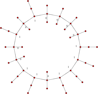
Figure 3.4. The graph $G_{n}$ is constructed from a de Bruijn sequence of length $2^{n}$.

It is easy to define a graphing $\mathbf{G}$, which is the limit of the sequence $(G_{n})_{n\in\mathbb{N}}$: as vertex set, we consider the rectangle $[0;1)\times[0;3)$. We define a measure preserving function $f$ and two measure preserving involutions $T_{1},T_{2}$ as follows:

$$f(x,y) =\begin{cases}(2x,y/2)&\text{if }x<1/2\text{ and }y<1\\ (2x-1,(y+1)/2)&\text{if }1/2\leq x\text{ and }y<1\\ (x,y)&\text{otherwise}\end{cases}$$

$$T_{1}(x,y) =\begin{cases}(x,y+1)&\text{if }y<1\\ (x,y-1)&\text{if }1\leq y<2\\ (x,y)&\text{otherwise}\end{cases}$$

$$T_{2}(x,y) =\begin{cases}(x,y+1)&\text{if }x<1/2\text{ and }1\leq y<2\\ (x,y+2)&\text{if }1/2\leq x\text{ and }y<1\\ (x,y-1)&\text{if }x<1/2\text{ and }2\leq y\\ (x,y-2)&\text{if }1/2\leq x\text{ and }2\leq y\\ (x,y)&\text{otherwise}\end{cases}$$

Then the edges of $\mathbf{G}$ are the pairs $\{(x,y),(x^{\prime},y^{\prime})\}$ such that $(x,y)\neq(x^{\prime},y^{\prime})$ and either $(x^{\prime},y^{\prime})=f(x,y)$, or $(x,y)=f(x^{\prime},y^{\prime})$, or $(x^{\prime},y^{\prime})=T_{1}(x,y)$, or $(x^{\prime},y^{\prime})=T_{2}(x,y)$.

If one considers a random root $(x,y)$ in $\mathbf{G}$, then the connected component of $(x,y)$ will almost surely be a rooted line with some decoration, as expected from what is seen from a random root in a sufficiently large $G_{n}$. However, special behaviour may happen when $x$ and $y$ are rational. Namely, it is possible that the connected component of $(x,y)$ becomes finite. For instance, if $x=1/(2^{n}-1)$ and $y=2^{n-1}x$ then the orbit of $(x,y)$ under the action of $f$ has length $n$; thus the connected component of $(x,y)$ in $\mathbf{G}$ has order $3n$. Of course, such finite connected components do not appear in $G_{n}$. Hence, in order to clean $\mathbf{G}$, infinitely many components have to be removed.

Let us give a simple example exemplifying the distinction between BS and ${\rm FO}$-convergence for graphs with bounded degree.

Example 3.48.

Let $G_{n}$ denote the $n\times n$ grid. The BS-limit object is a probability distribution concentrated on the infinite grid with a specified root. A limit graphing can be described as the Lebesgue measure on $[0,1]^{2}$, where $(x,y)$ is adjacent to $(x\pm\alpha\bmod 1,y\pm\alpha\bmod 1)$ for some irrational number $\alpha$.

This graphing, however, is not an ${\rm FO}$-limit of the sequence $(G_{n})_{n\in\mathbb{N}}$ as every ${\rm FO}$-limit has to contain four vertices of degree $2$. An ${\rm FO}$-limit graphing can be described as the above graphing restricted to $[0,1)^{2}$ (obtained by deleting all vertices with $x=1$ or $y=1$). One checks for instance that this graphing contains four vertices of degree $2$ (the vertices $(\alpha,\alpha)$, $(1-\alpha,\alpha)$, $(\alpha,1-\alpha)$, and $(1-\alpha,1-\alpha)$) and infinitely many vertices of degree $3$.

We want to stress that our general and unifying approach to structural limits was not developed for its own sake and that it provided a proper setting (and, yes, encouragement) for the study of classes of sparse graphs. So far classes of graphs with bounded degree are the only classes of sparse graphs where the structural limits were constructed efficiently. (Another example of limits of sparse graphs is provided by scaling limits of transitive graphs [9] which proceeds in different direction and is not considered here.)

3.3. Decomposing Sequences: the Comb Structure

The combinatorics of limits of equivalence relations (such as components) is complicated. We start this analysis by considering the combinatorics of “large” equivalence classes. This leads to the notion of spectrum, which will be analyzed in this section.

3.3.1. Spectrum of a First-order Equivalence Relation

Definition 3.49 ($\varpi$-spectrum).

Let $\mathbf{A}$ be a $\lambda$-modeling (with measure $\nu_{\mathbf{A}}$), and let $\varpi\in{\rm FO}_{2}(\lambda)$ be a formula expressing a component relation on $\mathbf{A}$ (see Definition 2.24). Let $\{C_{i}:i\in\Gamma\}$ be the set of all the $\varpi$-equivalence classes of $A$, and let $\Gamma_{+}$ be the (countable) subset of $\Gamma$ of the indexes $i$ such that $\nu_{\mathbf{A}}(C_{i})>0$.

The $\varpi$-spectrum ${\rm Sp}_{\varpi}(\mathbf{A})$ of $\mathbf{A}$ is the (countable) sequence of the values $\nu_{\mathbf{A}}(C_{i})$ (for $i\in\Gamma_{+}$) ordered in non-increasing order.

Lemma 3.50.

For $k\in\mathbb{N}$, let $\varpi^{(k)}$ be the formula $\bigwedge_{i=1}^{k}\varpi(x_{i},x_{i+1})$. Then the following equation holds:

$$\sum_{i\in\Gamma_{+}}\nu_{\mathbf{A}}(C_{i})^{k+1}=\langle\varpi^{(k)},\mathbf{A}\rangle.$$

Proof.

Let $k\in\mathbb{N}$. Define

$$D_{k+1}=\{(x_{1},\dots,x_{k+1})\in A^{k+1}:\ A\models\varpi^{k}(x_{1},\dots,x_{k+1})\}.$$

According to Lemma 3.3, each $C_{i}$ is measurable, thus $\bigcup_{i\in\Gamma_{+}}C_{i}$ is measurable and so is $R=A\setminus\bigcup_{i\in\Gamma_{+}}C_{i}$.

Considering the indicator function $\mathbf{1}_{D_{k+1}\cap R^{k+1}}$ of $D_{k+1}\cap R^{k+1}$ and applying Fubini’s theorem, we get

$$\int_{A^{k+1}}\mathbf{1}_{D_{k+1}\cap R^{k+1}}\,{\rm d}\nu_{\mathbf{A}}^{k+1}=\idotsint\mathbf{1}_{R}(x_{1},\dots,x_{k+1})\ {\rm d}\nu_{\mathbf{A}}(x_{1},\dots,{\rm d}\nu_{\mathbf{A}}(x_{k+1})=0.$$

as for every fixed $a_{1},\dots,a_{k}$ (with $a_{1}\in C_{\alpha}$, for some $\alpha\in\Gamma\setminus\Gamma_{+}$) we have

$$0\leq\int\mathbf{1}_{R}(a_{1},\dots,a_{k},x_{k+1})\,{\rm d}\nu_{\mathbf{A}}(x_{k+1})\leq\nu_{\mathbf{A}}(C_{\alpha})=0.$$

It follows (by countable additivity) that

$$\langle\varpi^{(k)},\mathbf{A}\rangle=\nu_{\mathbf{A}}^{k+1}(D_{k+1})=\nu_{\mathbf{A}}^{k+1}(\bigcup_{i\in\Gamma_{+}}C_{i}^{k+1})=\sum_{i\in\Gamma_{+}}\nu_{\mathbf{A}}(C_{i})^{k+1}.$$

∎

It follows from Lemma 3.50 that the spectrum ${\rm Sp}_{\varpi}(\mathbf{A})$ is computable from the sequence of (non-increasing) values $(\langle\varpi^{(k)},\mathbf{A}\rangle)_{k\in\mathbb{N}}$.

We assume that every finite sequence $\mathbf{x}=(x_{1},\dots,x_{n})$ of positive reals is implicitly embedded in an infinite sequence by defining $x_{i}=0$ for $i>n$. Recall the usual $\ell_{k}$ norms:

$$\|\mathbf{x}\|_{k}=\Bigl{(}\sum_{i}|x_{i}|^{k}\Bigr{)}^{1/k}.$$

Hence above equations rewrite as

(3.1) $$\|{\rm Sp}_{\varpi}(\mathbf{A})\|_{k+1}=\langle\varpi^{(k)},\mathbf{A}\rangle^{1/(k+1)}.$$

We shall prove that the spectrum is, in a certain sense, defined by a continuous function. We need the following technical lemma.

Lemma 3.51.

For each $n\in\mathbb{N}$, let $\mathbf{a}_{n}=(a_{n,i})_{i\in\mathbb{N}}$ be a non-increasing sequence of positive real numbers with bounded sum (i.e $\|\mathbf{a}_{n}\|_{1}<\infty$ for every $n\in\mathbb{N}$).

Assume that for every integer $k\geq 1$ the limit $s_{k}=\lim_{n\rightarrow\infty}\|\mathbf{a}_{n}\|_{k}$ exists.

Then $(\mathbf{a}_{n})_{n\in\mathbb{N}}$ converges in the space $c_{0}$ of all sequences converging to zero (with norm $\|\,\cdot\,\|_{\infty}$).

Proof.

We first prove that the sequences converge pointwise, that is that there exists a sequence $\mathbf{x}=(x_{i})_{i\in\mathbb{N}}$ such that for every $i\in\mathbb{N}$ the following equation holds:

$$x_{i}=\lim_{n\rightarrow\infty}a_{n,i}.$$

For every $\epsilon>0$, if $s_{k}<\epsilon$ then $a_{n,1}<2\epsilon$ for all sufficiently large values of $n$. Thus if $s_{k}=0$ for some $k$, the limit $\lim_{n\rightarrow}a_{n,i}$ exists for every $i$ and is null. Thus, we can assume that $s_{k}$ is strictly positive for every $k\in\mathbb{N}$.

Fix $k\in\mathbb{N}$. There exists $N\in\mathbb{N}$ such that for every $n\geq N$ it holds that $|s_{k}^{k}-\|\mathbf{a}_{n}\|_{k}^{k}|<s_{k}^{k}/k$. As $(a_{n,i})_{i\in\mathbb{N}}$ is a non-increasing sequence of positive real numbers, for every $n\neq N$ the following inequality holds

$$a_{n,1}^{k}\leq\|\mathbf{a}_{n}\|_{k}^{k}<s_{k}^{k}(1+1/k)$$

and

$$a_{n,1}^{k-1}\geq\|\mathbf{a}_{n}\|_{k}^{k}>s_{k}^{k}(1-1/k).$$

Hence

$$\log s_{k}+\frac{\log(1+1/k)}{k}\geq\log a_{n,1}\geq\bigl{(}1+\frac{1}{k-1}\bigr{)}\bigl{(}\log s_{k}+\frac{\log(1-1/k)}{k}\bigr{)}.$$

Thus $x_{1}=\lim_{n\rightarrow\infty}a_{n,1}$ exists and $x_{1}=\lim_{k\rightarrow\infty}s_{k}$. Inductively, we get that for each $i\in\mathbb{N}$, the limit $x_{i}=\lim_{n\rightarrow\infty}a_{n,i}$ exists and that

$$x_{i}=\lim_{k\rightarrow\infty}(s_{k}^{k}-\sum_{j<i}x_{j}^{k})^{1/k}.$$

We now prove that the converge is uniform, that is that for every $\epsilon>0$ there exists $N$ such that for every $n\geq N$ the following inequality holds:

$$\|\mathbf{x}-\mathbf{a}_{n}\|_{\infty}<\epsilon.$$

As $\mathbf{a}_{n}\in\ell_{1}$ and $\|\mathbf{a}_{n}\|_{1}$ converges there exists $M$ such that $\|\mathbf{a}_{n}\|_{1}\leq M$ for every $n\in\mathbb{N}$. Let $\epsilon>0$. Let $A=\min\{i:x_{i}\leq\epsilon/3\}$. (Note that $A\leq 3M/\epsilon$.) There exists $N$ such that for every $n\geq N$ it holds that $\sup_{i\leq A}|x_{i}-a_{n,i}|<\epsilon/3$. Moreover, for every $i>A$ the following inequality holds:

$$0\leq a_{n,i}\leq a_{n,A}<x_{A}+\epsilon/3<2\epsilon/3.$$

As $0\leq x_{i}\leq\epsilon/3$ for every $i>A$ the following inequality holds:

$$|x_{i}-a_{n,i}|<\epsilon$$

for every $i>A$ (hence for every $i$). Thus $(\mathbf{a}_{n})_{n\in\mathbb{N}}$ converges in $\ell_{\infty}$. As obviously each $\mathbf{a}_{n}$ has $0$ limit, $(\mathbf{a}_{n})_{n\in\mathbb{N}}$ converges in $c_{0}$. ∎

Lemma 3.52.

Let $\lambda$ be a signature. The mapping $\mathbf{A}\mapsto{\rm Sp}_{\varpi}(\mathbf{A})$ is a continuous mapping from the space of $\lambda$-modelings with a component relation $\varpi$ (with the topology of ${\rm FO}^{\rm local}(\lambda)$-convergence) to the space $c_{0}$ of all sequences converging to zero (with $\|\,\cdot\,\|_{\infty}$ norm).

Proof.

Assume $\mathbf{A}_{n}$ is an ${\rm FO}^{\rm local}(\lambda)$-convergent sequence of $\lambda$-modelings.

Let $(\hskip 1.0pt\mathsf{sp}_{n,1},\dots,\hskip 1.0pt\mathsf{sp}_{n,i},\dots)$ be the $\varpi$-spectrum of $\mathbf{A}_{n}$ (extended by zero values if finite), and let $\mathbf{a}_{n}=(a_{n,i})_{i\in\mathbb{N}}$ be the sequence defined by $a_{n,i}=\hskip 1.0pt\mathsf{sp}_{n,i}^{2}$. Then for every integer $k\geq 1$ it holds that

$$\|a_{n}\|_{k}=\|{\rm Sp}_{\varpi}(\mathbf{A}_{n})\|_{2k}^{2}=\langle\varpi^{(2k-1)},\mathbf{A}_{n}\rangle^{1/k}.$$

Hence $s_{k}=\lim_{n\rightarrow\infty}\|a_{n}\|_{k}$ exists. According to Lemma 3.51, $(\mathbf{a}_{n})_{n\in\mathbb{N}}$ converges in $c_{0}$, thus so does $({\rm Sp}_{\varpi}(\mathbf{A}_{n}))_{n\in\mathbb{N}}$. ∎

Definition 3.53.

Let $(\mathbf{A}_{n})_{n\in\mathbb{N}}$ be a sequence of finite $\lambda$-structures. Let $\varpi$ be a component relation, and for simplicity assume $\varpi\in\lambda$. In the following, we assume that $\varpi$-spectra are extended to infinite sequences by adding zeros if necessary.

• The sequence $(\mathbf{A}_{n})_{n\in\mathbb{N}}$ is $\varpi$-nice if ${\rm Sp}_{\varpi}(\mathbf{A}_{n})$ converges pointwise;

• The limit $\varpi$-spectrum of a $\varpi$-nice sequence $(\mathbf{A}_{n})_{n\in\mathbb{N}}$ is the pointwise limit of ${\rm Sp}_{\varpi}(\mathbf{A}_{n})$;

• the $\varpi$-support is the set $I$ of the indexes $i$ for which the limit $\varpi$-spectrum is non-zero;

• the sequence has full $\varpi$-spectrum if, for every index $i$ not in the $\varpi$-support, there is some $N$ such that the $i$th value of ${\rm Sp}_{\varpi}(\mathbf{A}_{n})$ is zero for every $n>N$.

As proved in Lemma 3.52, every ${\rm FO}^{\rm local}$-convergent sequence is $\varpi$-nice.

Lemma 3.54.

Let $(\mathbf{A}_{n})$ be a $\varpi$-nice sequence of $\lambda$-structures with empty $\varpi$-support.

Then the following conditions are equivalent:

1. the sequence $(\mathbf{A}_{n})$ is ${\rm FO}^{\rm local}$-convergent;

2. the sequence $(\mathbf{A}_{n})$ is ${\rm FO}_{1}^{\rm local}$-convergent.

Moreover, for every $\varpi$-local formula $\phi$ with $p>1$ free variables it holds that

$$\lim_{n\rightarrow\infty}\langle\phi,\mathbf{A}_{n}\rangle=0.$$

Proof.

${\rm FO}^{\rm local}$-convergence obviously implies ${\rm FO}_{1}^{\rm local}$-convergence. So, assume that $(\mathbf{A}_{n})_{n\in\mathbb{N}}$ is ${\rm FO}_{1}^{\rm local}$-convergent, and let $\phi$ be a $\varpi$-local first-order formula with $p>1$ free variables. For $n\in\mathbb{N}$, let $\mathbf{B}_{n,i}$ ($i\in\Gamma_{n}$) denote the connected components of $\mathbf{A}_{n}$. As $(\mathbf{A}_{n})$ is $\varpi$-nice and has empty $\varpi$-support, there exists for every $\epsilon>0$ an integer $N$ such that for $n>N$ and every $i\in\Gamma_{n}$ it holds that $|B_{n,i}|<\epsilon|A_{n}|$. Then, according to Corollary 3.21, for $n>N$

$$\langle\phi,\mathbf{A}_{n}\rangle =\sum_{i\in\Gamma_{n}}\biggl{(}\frac{|B_{n,i}|}{|A_{n}|}\biggr{)}^{p}\langle\phi,\mathbf{B}_{n,i}\rangle$$

$$\leq\sum_{i\in\Gamma_{n}}\biggl{(}\frac{|B_{n,i}|}{|A_{n}|}\biggr{)}^{p}$$

$$<\sum_{i\in\Gamma_{n}}\frac{|B_{n,i}|}{|A_{n}|}\epsilon^{p-1}=\epsilon^{p-1}.$$

Hence $\langle\phi,\mathbf{A}_{n}\rangle$ converges (to $0$) as $n$ grows to infinity. It follows that $(\mathbf{A}_{n})_{n\in\mathbb{N}}$ is ${\rm FO}^{\rm local}$-convergent, according to Theorem 3.22. ∎

Lemma 3.55.

Let $(\mathbf{A}_{n})_{n\in\mathbb{N}}$ be an ${\rm FO}^{\rm local}$-convergent sequence of finite $\lambda$-structures, with component relation $\varpi\in\lambda$ and limit $\varpi$-spectrum $(\hskip 1.0pt\mathsf{sp}_{i})_{i\in I}$. For $n\in\mathbb{N}$, let $\mathbf{B}_{n,i}$ be the connected components of $\mathbf{A}_{n}$ order in non-decreasing order (with $\mathbf{B}_{n,i}$ empty if $i$ is greater than the number of connected components of $\mathbf{A}_{n}$). Let $a\leq b$ be the first and last occurrence of $\hskip 1.0pt\mathsf{sp}_{a}=\hskip 1.0pt\mathsf{sp}_{b}$ in the $\varpi$-spectrum and let $\mathbf{A}_{n}^{\prime}$ be the union of all the $\mathbf{B}_{n,i}$ for $a\leq i\leq b$.

Then $(\mathbf{A}_{n}^{\prime})_{n\in\mathbb{N}}$ is ${\rm FO}$-convergent if $\hskip 1.0pt\mathsf{sp}_{a}>0$ and ${\rm FO}^{\rm local}$-convergent if $\hskip 1.0pt\mathsf{sp}_{a}=0$.

Assume moreover that $(\mathbf{A}_{n})_{n\in\mathbb{N}}$ has a modeling ${\rm FO}^{\rm local}$-limit ${\mathbf{L}}$. Let $\mathbf{L}^{\prime}$ be the union of the connected components $\mathbf{L}_{i}$ of $\mathbf{L}$ with $\nu_{\mathbf{L}}(L_{i})=\hskip 1.0pt\mathsf{sp}_{a}$. Equip $\mathbf{L}^{\prime}$ with the $\sigma$-algebra $\Sigma_{\mathbf{L}^{\prime}}$ which is the restriction of $\Sigma_{\mathbf{L}}$ to $L^{\prime}$ and the probability measure $\nu_{\mathbf{L}^{\prime}}$ defined by $\nu_{\mathbf{L}^{\prime}}(X)=\nu_{\mathbf{L}}(X)/\nu_{\mathbf{L}}(L^{\prime})$ (for $X\in\Sigma_{\mathbf{L}^{\prime}}$).

Then $\mathbf{L}^{\prime}$ is a modeling ${\rm FO}$-limit of $(\mathbf{A}_{n}^{\prime})_{n\in\mathbb{N}}$ if $\hskip 1.0pt\mathsf{sp}_{a}>0$ and a modeling ${\rm FO}^{\rm local}$-limit of $(\mathbf{A}_{n}^{\prime})_{n\in\mathbb{N}}$ if $\hskip 1.0pt\mathsf{sp}_{a}=0$.

Proof.

Extend the sequence $\hskip 1.0pt\mathsf{sp}$ to the null index by defining $\hskip 1.0pt\mathsf{sp}_{0}=2$. Let $r=\min(\hskip 1.0pt\mathsf{sp}_{a-1}/\hskip 1.0pt\mathsf{sp}_{a},\hskip 1.0pt\mathsf{sp}_{b}/\hskip 1.0pt\mathsf{sp}_{b+1})$ (if $\hskip 1.0pt\mathsf{sp}_{b+1}=0$ simply define $r=\hskip 1.0pt\mathsf{sp}_{a-1}/\hskip 1.0pt\mathsf{sp}_{a}$). Notice that $r>1$. Let $\phi$ be a $\varpi$-local formula with $p$ free variables. According to Corollary 3.21 the following equation holds:

$$\langle\phi,\mathbf{A}_{n}\rangle=\sum_{i}\biggl{(}\frac{|B_{n,i}|}{|A_{n}|}\biggr{)}^{p}\langle\phi,\mathbf{B}_{n,i}\rangle.$$

In particular, it holds that

$$\langle\varpi^{(p)},\mathbf{A}_{n}\rangle=\sum_{i}\left(\frac{|B_{n,i}|}{|A_{n}|}\right)^{p}.$$

Let $\alpha>1/(1-r^{p})$. Define

$$w_{n,i}=\biggl{(}\frac{|B_{n,i}|}{|A_{n}|}\biggr{)}^{p}(\alpha+\langle\phi,\mathbf{B}_{n,i}\rangle).$$

From the definition of $r$ it follows that for each $n\in\mathbb{N}$, $w_{n,i}>w_{n,j}$ if $i<a$ and $j\geq a$ or $i\leq b$ and $j>b$. Let $\sigma\in\mathfrak{S}_{\omega}$ be a permutation of $\mathbb{N}$, such that $a_{n,i}=w_{n,\sigma(i)}$ is non-increasing. It holds that

$$\sum_{i}a_{n,i}=\sum_{i}w_{n,i}=\alpha\langle\varpi^{(p)},\mathbf{A}_{n}\rangle+\langle\phi,\mathbf{A}_{n}\rangle.$$

Hence

$$\lim_{n\rightarrow\infty}\sum_{i}a_{n,i}^{p}$$

exists. According to Lemma 3.51 it follows that for every $i\in\mathbb{N}$ the limit $\lim_{n\rightarrow\infty}a_{n,i}$ exists. Moreover, as $\sigma$ globally preserves the set $\{a,\dots,b\}$ it follows that the limit

$$d=\lim_{n\rightarrow\infty}\sum_{i=a}^{b}\biggl{(}\frac{|B_{n,i}|}{|A_{n}|}\biggr{)}^{p}(\alpha+\langle\phi,\mathbf{B}_{n,i}\rangle)$$

exists. As for every $i\in\{a,\dots,b\}$ it holds that $\lim_{n\rightarrow\infty}|B_{n,i}|/|A_{n}|=\hskip 1.0pt\mathsf{sp}_{a}$ and as $\langle\phi,\mathbf{A}_{n}^{\prime}\rangle=\sum_{i=a}^{b}(|B_{n,i}|/|A_{n}|)^{p}\langle\phi,\mathbf{B}_{n,i}\rangle$ we deduce

$$\lim_{n\rightarrow\infty}\langle\phi,\mathbf{A}_{n}^{\prime}\rangle=d-(b-a+1)\alpha.$$

Hence $\lim_{n\rightarrow\infty}\langle\phi,\mathbf{A}_{n}^{\prime}\rangle$ exists for every $\varpi$-local formula and, according to Theorem 3.22, the sequence $(\mathbf{A}_{n}^{\prime})_{n\in\mathbb{N}}$ is ${\rm FO}^{\rm local}$-convergent.

Assume $\hskip 1.0pt\mathsf{sp}_{a}>0$. Let $N=b-a+1$. To each sentence $\theta$ we associate the formula $\widetilde{\theta}\in{\rm FO}_{N}^{\rm local}$ that asserts that the substructure induced by the closed neighborhood of $x_{1},\dots,x_{N}$ satisfies $\theta$ and that $x_{1},\dots,x_{N}$ are pairwise distinct and non-adjacent. For sufficiently large $n$, the structure $\mathbf{A}_{n}^{\prime}$ has exactly $N$ connected components. It is easily checked that if $\mathbf{A}_{n}^{\prime}$ does not satisfy $\theta$ then $\langle\widetilde{\theta},\mathbf{A}_{n}^{\prime}\rangle=0$, although if $\mathbf{A}_{n}^{\prime}$ does satisfy $\theta$ then

$$\langle\widetilde{\theta},\mathbf{A}_{n}^{\prime}\rangle\geq\Bigl{(}\frac{\min_{a\leq i\leq b}|B_{n,i}|}{\sum_{i=a}^{b}|B_{n,i}|}\Bigr{)}^{N},$$

hence $\langle\widetilde{\theta},\mathbf{A}_{n}^{\prime}\rangle>(2N)^{-N}$ for all sufficiently large $n$. As $\langle\widetilde{\theta},\mathbf{A}_{n}^{\prime}\rangle$ converges for every sentence $\theta$, we deduce that the sequence $(\mathbf{A}_{n}^{\prime})_{n\in\mathbb{N}}$ is elementarily convergent. According to Theorem 2.23, the sequence $(\mathbf{A}_{n}^{\prime})_{n\in\mathbb{N}}$ is thus ${\rm FO}$-convergent.

Now assume that $(\mathbf{A}_{n})_{n\in\mathbb{N}}$ has a modeling ${\rm FO}^{\rm local}$-limit ${\mathbf{L}}$. First note that $L_{i}$ being an equivalence class of $\varpi$ it holds that $L_{i}\in\Sigma_{\mathbf{L}}$, hence $L^{\prime}\in\Sigma_{\mathbf{L}}$ and $\nu_{\mathbf{L}}(L^{\prime})$ is well defined. For every $\varpi$-local formula $\phi\in{\rm FO}_{p}(\lambda)$ it holds, according to Lemma 3.20, that

$$\langle\phi,\mathbf{L}^{\prime}\rangle =\sum_{i=a}^{b}\nu_{\mathbf{L}^{\prime}}(L_{i})^{p}\langle\phi,\mathbf{L}_{i}\rangle$$

$$=\frac{1}{\nu_{\mathbf{L}}(L^{\prime})^{p}}\sum_{i=a}^{b}\nu_{\mathbf{L}}(L_{i})^{p}\langle\phi,\mathbf{L}_{i}\rangle.$$

We deduce that

$$\langle\phi,\mathbf{L}^{\prime}\rangle=\lim_{n\rightarrow\infty}\langle\phi,\mathbf{A}_{n}^{\prime}\rangle.$$

According to Theorem 3.22, it follows that the same equality holds for every $\phi\in{\rm FO}^{\rm local}(\lambda)$ hence $\mathbf{L}^{\prime}$ is a modeling ${\rm FO}^{\rm local}$-limit of the sequence $(\mathbf{A}_{n}^{\prime})_{n\in\mathbb{N}}$.

As above, for $\hskip 1.0pt\mathsf{sp}_{a}>0$, if $\mathbf{L}^{\prime}$ is a modeling ${\rm FO}^{\rm local}$-limit of $(\mathbf{A}_{n}^{\prime})_{n\in\mathbb{N}}$ then it is a modeling ${\rm FO}$-limit.

∎

Lemma 3.56.

Let $(\mathbf{A}_{n})_{n\in\mathbb{N}}$ be an ${\rm FO}$-convergent sequence of finite $\lambda$-structures, with component relation $\varpi$ (expressing usual notion of connected components). Assume all the $\mathbf{A}_{n}$ have at most $k$ connected components. Denote by $\mathbf{B}_{n,1},\dots,\mathbf{B}_{n,k}$ these components (adding empty $\lambda$-structures if necessary).

Assume that for each $1\leq i\leq k$ it holds that $\lim_{n\rightarrow\infty}|B_{n,i}|/|A_{n}|=1/k$.

Then there exists a sequence $(\sigma_{n})_{n\in\mathbb{N}}$ of permutations of $[k]$ such that for each $1\leq i\leq k$ the sequence $(\mathbf{B}_{n,\sigma_{n}(i)})_{n\in\mathbb{N}}$ is ${\rm FO}$-convergent.

Proof.

To a formula $\phi\in{\rm FO}_{p}(\lambda)$ we associate the $\varpi$-local formula $\widetilde{\phi}\in{\rm FO}_{p}^{\rm local}(\lambda)$ asserting that all the free variables are $\varpi$-adjacent and that their closed neighborhood (that is their connected component) satisfies $\phi$. Then essentially the same proof as above allows to refine $\mathbf{A}_{n}$ into sequences such that $\langle\phi,\mathbf{A}_{n,i}^{\prime}\rangle$ is constant on the connected components of each of the $\mathbf{A}_{n}^{\prime}$. Considering formulas allowing to split at least one of the sequences, we repeat this process (at most $k-1$ times) until each $\mathbf{A}_{n,i}^{\prime}$ contains equivalent connected components. Then, $\mathbf{A}_{n,i}^{\prime}$ can be split into connected components in an arbitrary order, thus obtaining the sequences $\mathbf{B}_{n,i}$. ∎

So we have proved that a ${\rm FO}$-convergent can be decomposed by isolines of the $\varpi$-spectrum (that is by groups of connected components with same asymptotic measure). In the next sections, we shall investigate how to refine this further.

3.3.2. Sequences with Finite Spectrum

For every $\varpi$-nice sequence $(\mathbf{A}_{n})_{n\in\mathbb{N}}$ with finite support $I$, we define the residue $\mathbf{R}_{n}$ of $\mathbf{A}_{n}$ as the union of the connected components $\mathbf{B}_{n,i}$ of $\mathbf{A}_{n}$ such that $i\notin I$.

When one considers an ${\rm FO}^{\rm local}$-convergent sequence $(\mathbf{A}_{n})$ with a finite support then the sequence of the residues forms a sequence which is either ${\rm FO}^{\rm local}$-convergent or “negligible” in the sense that $\lim_{n\rightarrow\infty}|R_{n}|/|A_{n}|=0$. This is formulated as follows:

Lemma 3.57.

Let $(\mathbf{A}_{n})_{n\in\mathbb{N}}$ be a sequence of $\lambda$-structures with component relation $\varpi$. For each $n\in\mathbb{N}$ and $i\in\mathbb{N}$, let $\mathbf{B}_{n,i}$ be the $i$-th largest connected component of $\mathbf{A}_{n}$.

Assume that $(\mathbf{A}_{n})_{n\in\mathbb{N}}$ is ${\rm FO}^{\rm local}$-convergent and has finite spectrum $(\hskip 1.0pt\mathsf{sp}_{i})_{i\in I}$. Let $\mathbf{R}_{n}$ be the residue of $\mathbf{A}_{n}$.

Then $\hskip 1.0pt\mathsf{sp}^{\prime}=\lim_{n\rightarrow\infty}|R_{n}|/|A_{n}|$ exists and either $\hskip 1.0pt\mathsf{sp}^{\prime}=0$ or $(\mathbf{R}_{n})_{n\in\mathbb{N}}$ is ${\rm FO}^{\rm local}$-convergent.

Proof.

Clearly, $\hskip 1.0pt\mathsf{sp}^{\prime}=1-\sum_{i}\hskip 1.0pt\mathsf{sp}_{i}$. Assume $\hskip 1.0pt\mathsf{sp}^{\prime}>0$. First notice that for every $\epsilon>0$ there exists $N$ such that for every $i>N$, the $\lambda$-structure $\mathbf{R}_{n}$ has no connected component of size at least $\epsilon/2\hskip 1.0pt\mathsf{sp}^{\prime}|A_{n}|$ and $\mathbf{R}_{n}$ has order at least $\hskip 1.0pt\mathsf{sp}^{\prime}/2|A_{n}|$. Hence, for every $i>N$, the $\lambda$-structure $\mathbf{R}_{n}$ has no connected component of size at least $\epsilon|R_{n}|$. According to Lemma 3.54, proving that $(\mathbf{R}_{n})_{n\in\mathbb{N}}$ is ${\rm FO}^{\rm local}$-convergent reduces to proving that $(\mathbf{R}_{n})_{n\in\mathbb{N}}$ is ${\rm FO}_{1}^{\rm local}$-convergent.

Let $\phi\in{\rm FO}_{1}^{\rm local}$. We group the $\lambda$-structures $\mathbf{B}_{n,i}$ (for $i\in I$) by values of $\hskip 1.0pt\mathsf{sp}_{i}$ as $\mathbf{A}_{n,1}^{\prime},\dots,\mathbf{A}_{n,q}^{\prime}$. Denote by $c_{j}$ the common value of $\hskip 1.0pt\mathsf{sp}_{i}$ for the connected components $\mathbf{B}_{n,i}$ in $\mathbf{A}_{n,j}^{\prime}$. According to Corollary 3.21 it holds (as $\phi$ is clearly $\varpi$-local) that

$$\langle\phi,\mathbf{A}_{n}\rangle =\sum_{i}\frac{|B_{n,i}|}{|A_{n}|}\langle\phi,\mathbf{B}_{n,i}\rangle$$

$$=\sum_{i\in I}\frac{|B_{n,i}|}{|A_{n}|}\langle\phi,\mathbf{B}_{n,i}\rangle+\sum_{i\notin I}\frac{|B_{n,i}|}{|A_{n}|}\langle\phi,\mathbf{B}_{n,i}\rangle$$

$$=\sum_{j=1}^{q}\frac{|A_{n,j}^{\prime}|}{|A_{n}|}\langle\phi,\mathbf{A}_{n,j}^{\prime}\rangle+\frac{|R_{n}|}{|A_{n}|}\langle\phi,\mathbf{R}_{n}\rangle.$$

According to Lemma 3.55, each sequence $(\mathbf{A}_{n,j}^{\prime})_{n\in\mathbb{N}}$ is ${\rm FO}$-convergent. Hence the limit $\lim_{n\rightarrow\infty}\langle\phi,\mathbf{R}_{n}\rangle$ exists and we have

$$\lim_{n\rightarrow\infty}\langle\phi,\mathbf{R}_{n}\rangle=\frac{1}{\hskip 1.0pt\mathsf{sp}^{\prime}}\biggl{(}\lim_{n\rightarrow\infty}\langle\phi,\mathbf{A}_{n}\rangle-\sum_{j=1}^{q}c_{j}\ \lim_{n\rightarrow\infty}\langle\phi,\mathbf{A}_{n,j}^{\prime}\rangle\biggr{)}.$$

It follows that the sequence $(\mathbf{R}_{n})_{n\in\mathbb{N}}$ is ${\rm FO}^{\rm local}$-convergent. ∎

The following result finally determines the structure of converging sequences of (disconnected) $\lambda$-structures with finite support. This structure is called comb structure, see Fig 3.5.

Theorem 3.58 (Comb structure for $\lambda$-structure sequences with finite spectrum).

Let $(\mathbf{A}_{n})_{n\in\mathbb{N}}$ be an ${\rm FO}^{\rm local}$-convergent sequence of finite $\lambda$-structures with component relation $\varpi$ and finite spectrum $(\hskip 1.0pt\mathsf{sp}_{i})_{i\in I}$. Let $\mathbf{R}_{n}$ be the residue of $\mathbf{A}_{n}$.

Then there exists, for each $n\in\mathbb{N}$, a permutation $f_{n}:I\rightarrow I$ such that the following holds

• $\lim_{n\rightarrow\infty}\max_{i\notin I}|B_{n,i}|/|A_{n}|=0$;

• $\lim_{n\rightarrow\infty}|R_{n}|/|A_{n}|$ exists;

• for every $i\in I$, the sequence $(B_{n,f_{n}(i)})_{n\in\mathbb{N}}$ is ${\rm FO}$-convergent and $\lim_{n\rightarrow\infty}|B_{n,f_{n}(i)}|/|A_{n}|=\hskip 1.0pt\mathsf{sp}_{i}$;

• either $\lim_{n\rightarrow\infty}|R_{n}|/|A_{n}|=0$, or the sequence $(\mathbf{R}_{n})_{n\in\mathbb{N}}$ is ${\rm FO}^{\rm local}$-convergent.

Moreover, if $(\mathbf{A}_{n})_{n\in\mathbb{N}}$ is ${\rm FO}$-convergent then $(\mathbf{R}_{n})_{n\in\mathbb{N}}$ is elementary-convergent.

Proof.

This lemma is a direct consequence of Lemmas 3.55, 3.56 and 3.57, except that we still have to prove ${\rm FO}$-convergence of $(\mathbf{R}_{n})_{n\in\mathbb{N}}$ in the case where $(\mathbf{A}_{n})_{n\in\mathbb{N}}$ is ${\rm FO}$-convergent. As $I$ is finite, the elementary convergence of $(\mathbf{R}_{n})_{n\in\mathbb{N}}$ easily follows from the one of $(\mathbf{A}_{n})$ and the one of the $(\mathbf{B}_{n,f_{n}(i)})$ for $i\in I$. ∎

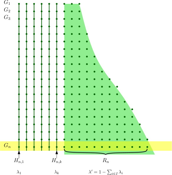
Figure 3.5. Illustration of the Comb structure for sequences with finite support

3.3.3. Sequences with Infinite Spectrum

Let $(\mathbf{A}_{n})_{n\in\mathbb{N}}$ be a $\varpi$-nice sequence with infinite spectrum (and support $I=\mathbb{N}$). In such a case, the notion of a residue becomes more tricky and will need some technical definitions. Before this, let us take the time to give an example illustrating the difficulty of the determination of the residue $\mathbf{R}_{n}$ in the comb structure of sequences with infinite spectrum.

Example 3.59.

Consider the sequence $(G_{n})_{n\in\mathbb{N}}$ where $G_{n}$ is the union of $2^{n}$ stars $H_{n,1},\dots,H_{n,2^{n}}$, where the $i$-th star $H_{n,i}$ has order $2^{2^{n}}(2^{-i}+2^{-n})/2$. Then it holds that

$$\hskip 1.0pt\mathsf{sp}_{i}=\lim_{n\rightarrow\infty}|H_{n,i}|/|G_{n}|=2^{-(i+1)}$$

hence $\sum_{i}\hskip 1.0pt\mathsf{sp}_{i}=1/2$ thus the residue asymptotically should contain half of the vertices of $G_{n}$! An ${\rm FO}$-limit of this sequence is shown Fig. 3.6.

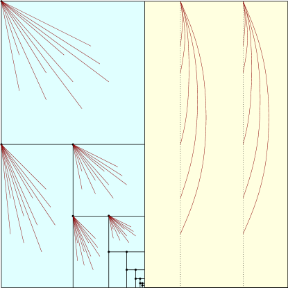
Figure 3.6. An ${\rm FO}^{\rm local}$-limit. On the left side, each rectangle correspond to a star with the upper left point as its center; on the right side, each vertical line is a star with the upper point as its center.

This example is not isolated. In fact it is quite frequent in many of its variants. To decompose such examples we need a convenient separation. This is provided by the notion of clip.

Definition 3.60.

• A clip of a $\varpi$-nice sequence $(\mathbf{A}_{n})_{n\in\mathbb{N}}$ with support $\mathbb{N}$ is a non-decreasing function $C:\mathbb{N}\rightarrow\mathbb{N}$ such that $\lim_{n\rightarrow\infty}C(n)=\infty$ and

  $$\forall n^{\prime}\geq n\quad\sum_{i=1}^{C(n)}\biggl{|}\frac{|B_{n^{\prime},i}|}{|A_{n^{\prime}}|}-\hskip 1.0pt\mathsf{sp}_{i}\biggr{|}\leq\sum_{i>C(n)}\hskip 1.0pt\mathsf{sp}_{i}$$

• The residue $\mathbf{R}_{n}$ of $\mathbf{A}_{n}$ with respect to a clip $C(n)$ is the disjoint union of the $\mathbf{B}_{n,i}$ for $i>C(n)$.

Proposition 3.61.

Every $\varpi$-nice sequence $(\mathbf{A}_{n})_{n\in\mathbb{N}}$ with infinite support has a clip $C_{0}$, which is defined by

$$C_{0}(n)=\sup\biggl{\{}M,\quad(\forall n^{\prime}\geq n)\ \sum_{i=1}^{M}\biggl{|}\frac{|B_{n^{\prime},i}|}{|A_{n^{\prime}}|}-\hskip 1.0pt\mathsf{sp}_{i}\biggr{|}\leq\sum_{i>M}\hskip 1.0pt\mathsf{sp}_{i}\biggr{\}}.$$

Moreover, $\lim_{n\rightarrow}C_{0}(n)=\infty$ and a non decreasing function $C$ is a clip of $(\mathbf{A}_{n})_{n\in\mathbb{N}}$ if and only if $C\leq C_{0}$ and $\lim_{n\rightarrow}C(n)=\infty$.

Proof.

Indeed, for each $n\in\mathbb{N}$, the value $z_{l}(M)=\sup_{n^{\prime}\geq n}\sum_{i=1}^{M}\biggl{|}\frac{|B_{n^{\prime},i}|}{|A_{n^{\prime}}|}-\hskip 1.0pt\mathsf{sp}_{i}\biggr{|}$ is non-decreasing function of $C$ with $z_{l}(0)=0$, and $z_{r}(M)=\sum_{i>M}\hskip 1.0pt\mathsf{sp}_{i}$ is a decreasing function of $C$ with $z_{r}(0)=\sum_{i}\hskip 1.0pt\mathsf{sp}_{i}>0$ hence $C_{0}$ is well defined. Moreover, for every integer $M$, let $\alpha=\sum_{i>M}\hskip 1.0pt\mathsf{sp}_{i}>0$. Then, as $\lim_{n\rightarrow\infty}|B_{n^{\prime},i}|/|A_{n^{\prime}}|=\hskip 1.0pt\mathsf{sp}_{i}$ there exists $N$ such that for every $n^{\prime}\geq N$ and every $1\leq i\leq M$ it holds that $||B_{n^{\prime},i}|/|A_{n^{\prime}}|-\hskip 1.0pt\mathsf{sp}_{i}|\leq\alpha/M$ thus for every $n^{\prime}\geq N$ it holds that

$$\sum_{i=1}^{M}\biggl{|}\frac{|B_{n^{\prime},i}|}{|A_{n^{\prime}}|}-\hskip 1.0pt\mathsf{sp}_{i}\biggr{|}\leq\alpha=\sum_{i>M}\hskip 1.0pt\mathsf{sp}_{i}.$$

It follows that $C_{0}(N)\geq M$. Hence $\lim_{n\rightarrow\infty}C_{0}(n)=\infty$.

That a non decreasing function $C$ is a clip of $(\mathbf{A}_{n})_{n\in\mathbb{N}}$ if and only if $C\leq C_{0}$ and $\lim_{n\rightarrow}C(n)=\infty$ follows directly from the definition. ∎

Lemma 3.62.

Let $(\mathbf{A}_{n})_{n\in\mathbb{N}}$ be a $\varpi$-nice sequence with support $\mathbb{N}$, and let $C$ be a clip of $(\mathbf{A}_{n})_{n\in\mathbb{N}}$.

Then the limit $\hskip 1.0pt\mathsf{sp}^{\prime}=\lim_{n\rightarrow\infty}\frac{|R_{n}|}{|A_{n}|}$ exists and $\hskip 1.0pt\mathsf{sp}^{\prime}=1-\sum_{i}\hskip 1.0pt\mathsf{sp}_{i}$.

Proof.

As $C$ is a clip, the following inequality holds for every $n\in\mathbb{N}$

$$\sum_{i}\hskip 1.0pt\mathsf{sp}_{i}-2\sum_{i>C(n)}\hskip 1.0pt\mathsf{sp}_{i}\leq\sum_{i=1}^{C(n)}\frac{|B_{n,i}|}{|A_{n}|}\leq\sum_{i}\hskip 1.0pt\mathsf{sp}_{i}.$$

Also, for every $\epsilon>0$ there exists $n$ such that $|\sum_{i=1}^{C(n)}\hskip 1.0pt\mathsf{sp}_{i}-\sum_{i}\hskip 1.0pt\mathsf{sp}_{i}|<\epsilon$, that is: $\sum_{i>C(n)}\hskip 1.0pt\mathsf{sp}_{i}<\epsilon.$ It follows that

$$\lim_{n\rightarrow\infty}\sum_{i=1}^{C(n)}\frac{|B_{n,i}|}{|A_{n}|}=\sum_{i}\hskip 1.0pt\mathsf{sp}_{i}.$$

Hence the limit $\hskip 1.0pt\mathsf{sp}^{\prime}=\lim_{n\rightarrow\infty}\frac{|R_{n}|}{|A_{n}|}$ exists and $\hskip 1.0pt\mathsf{sp}^{\prime}=1-\sum_{i}\hskip 1.0pt\mathsf{sp}_{i}$. ∎

Lemma 3.63.

Let $(\mathbf{A}_{n})_{n\in\mathbb{N}}$ be a sequence of $\lambda$-structures with component relation $\varpi$. For each $n\in\mathbb{N}$ and $i\in\mathbb{N}$, let $\mathbf{B}_{n,i}$ be the $i$-th largest connected component of $\mathbf{A}_{n}$ (if $i$ is at most equal to the number of connected components of $\mathbf{A}_{n}$, the empty $\lambda$-structure otherwise).

Assume that $(\mathbf{A}_{n})_{n\in\mathbb{N}}$ is ${\rm FO}$-convergent.

Let $C:\mathbb{N}\rightarrow\mathbb{N}$ be a clip of $(\mathbf{A}_{n})_{n\in\mathbb{N}}$, and let $\mathbf{R}_{n}$ be the residue of $\mathbf{A}_{n}$ with respect to $C$.

Let $\hskip 1.0pt\mathsf{sp}^{\prime}=\lim_{n\rightarrow\infty}|R_{n}|/|A_{n}|$. Then either $\hskip 1.0pt\mathsf{sp}^{\prime}=0$ or $(\mathbf{R}_{n})_{n\in\mathbb{N}}$ is ${\rm FO}^{\rm local}$-convergent.

Proof.

According to Lemma 3.62, $\lim_{n\rightarrow\infty}|R_{n}|/|A_{n}|$ exists and $\hskip 1.0pt\mathsf{sp}^{\prime}=1-\sum_{i}\hskip 1.0pt\mathsf{sp}_{i}$. Assume $\hskip 1.0pt\mathsf{sp}^{\prime}>0$. First notice that for every $\epsilon>0$ there exists $N$ such that for every $i>N$, the $\lambda$-structure $\mathbf{R}_{n}$ has no connected component of size at least $\epsilon/2\hskip 1.0pt\mathsf{sp}^{\prime}|\mathbf{A}_{n}|$ and $\mathbf{R}_{n}$ has order at least $\hskip 1.0pt\mathsf{sp}^{\prime}/2|A_{n}|$. Hence, for every $i>N$, the $\lambda$-structure $\mathbf{R}_{n}$ has no connected component of size at least $\epsilon|R_{n}|$. According to Lemma 3.54, proving that $(\mathbf{R}_{n})_{n\in\mathbb{N}}$ is ${\rm FO}^{\rm local}$-convergent reduces to proving that $(\mathbf{R}_{n})_{n\in\mathbb{N}}$ is ${\rm FO}_{1}^{\rm local}$-convergent.

Let $\phi\in{\rm FO}_{1}^{\rm local}$ (thus $\phi$ is $\varpi$-local). Let $\epsilon>0$. There exists $k\in\mathbb{N}$ such that $\sum_{i\leq k}\hskip 1.0pt\mathsf{sp}_{i}>1-\hskip 1.0pt\mathsf{sp}^{\prime}-\epsilon/3$ and such that $\hskip 1.0pt\mathsf{sp}_{k+1}<\hskip 1.0pt\mathsf{sp}_{k}$. We group the $\lambda$-structures $\mathbf{B}_{n,i}$ (for $1\leq i\leq k$) by values of $\hskip 1.0pt\mathsf{sp}_{i}$ as $\mathbf{A}_{n,1}^{\prime},\dots,\mathbf{A}_{n,q}^{\prime}$. Denote by $c_{j}$ the common value of $\hskip 1.0pt\mathsf{sp}_{i}$ for the connected components $\mathbf{B}_{n,i}$ in $\mathbf{A}_{n,j}^{\prime}$. According to Lemma 3.55, each sequence $(\mathbf{A}_{n,i}^{\prime})_{n\in\mathbb{N}}$ is ${\rm FO}$-convergent. Define

$$\mu_{i}=\lim_{n\rightarrow\infty}\langle\phi,\mathbf{A}_{n,i}^{\prime}\rangle.$$

There exists $N$ such that for every $n>N$ the following inequality holds

$$\sum_{i=1}^{q}|\langle\phi,\mathbf{A}_{n,i}^{\prime}\rangle-\mu_{i}|<\epsilon/3.$$

According to Corollary 3.21 it holds, for every $n>N$, that

$$\langle\phi,\mathbf{A}_{n}\rangle =\sum_{i}\frac{|B_{n,i}|}{|A_{n}|}\langle\phi,\mathbf{B}_{n,i}\rangle$$

$$=\sum_{i=1}^{k}\frac{|B_{n,i}|}{|A_{n}|}\langle\phi,\mathbf{B}_{n,i}\rangle+\sum_{i=k+1}^{C(n)}\frac{|A_{n,i}|}{|A_{n}|}\langle\phi,\mathbf{B}_{n,i}\rangle+\sum_{i>C(n)}\frac{|B_{n,i}|}{|A_{n}|}\langle\phi,\mathbf{B}_{n,i}\rangle$$

$$=\sum_{i=1}^{q}c_{i}\langle\phi,\mathbf{A}_{n,i}^{\prime}\rangle+\sum_{i=k+1}^{C(n)}\frac{|B_{n,i}|}{|A_{n}|}\langle\phi,\mathbf{B}_{n,i}\rangle+\frac{|R_{n}|}{|A_{n}|}\langle\phi,\mathbf{R}_{n}\rangle.$$

Thus we have

$$\biggl{|}\hskip 1.0pt\mathsf{sp}^{\prime}\langle\phi,\mathbf{R}_{n}\rangle-\bigl{(}\langle\phi,\mathbf{A}_{n}\rangle-\sum_{i=1}^{q}c_{i}\mu_{i}\bigr{)}\biggr{|} \leq\sum_{i=1}^{q}|\langle\phi,\mathbf{A}_{n,i}^{\prime}\rangle-\mu_{i}|+\sum_{i=k+1}^{C(n)}|B_{n,i}|/|A_{n}|$$

$$\quad+\bigl{|}|R_{n}|/|A_{n}|-\hskip 1.0pt\mathsf{sp}^{\prime}\bigr{|}$$

$$\leq\epsilon.$$

It follows that $\lim_{n\rightarrow\infty}\langle\phi,\mathbf{R}_{n}\rangle$ exists. By sorting the $C(n)$ first connected components of each $\mathbf{A}_{n}$ according to both $\hskip 1.0pt\mathsf{sp}_{i}$ and Lemma 3.56 we obtain the following expression for the limit:

$$\lim_{n\rightarrow\infty}\langle\phi,\mathbf{R}_{n}\rangle=\frac{1}{\hskip 1.0pt\mathsf{sp}^{\prime}}(\lim_{n\rightarrow\infty}\langle\phi,\mathbf{A}_{n}\rangle-\sum_{i<\widehat{C}}\hskip 1.0pt\mathsf{sp}_{i}\lim_{n\rightarrow\infty}\langle\phi,\mathbf{B}_{n,i}\rangle).$$

∎

Finally, we obtain the main results of this section.

Theorem 3.64 (Comb structure for $\lambda$-structure sequences with infinite spectrum (local convergence)).

Let $(\mathbf{A}_{n})_{n\in\mathbb{N}}$ be an ${\rm FO}^{\rm local}$-convergent sequence of finite $\lambda$-structures with component relation $\varpi$, support $\mathbb{N}$, and spectrum $(\hskip 1.0pt\mathsf{sp}_{i})_{i\in\mathbb{N}}$. Let $C:\mathbb{N}\rightarrow\mathbb{N}$ be a clip of $(\mathbf{A}_{n})_{n\in\mathbb{N}}$, and let $\mathbf{R}_{n}$ be the residue of $\mathbf{A}_{n}$ with respect to $C$.

Then there exists, for each $n\in\mathbb{N}$, a permutation $f_{n}:[C(n)]\rightarrow[C(n)]$ such that, extending $f_{n}$ to $\mathbb{N}$ by putting $f(i)$ to be the identity for $i>C(n)$, the following holds:

• $\lim_{n\rightarrow\infty}\max_{i>C(n)}|B_{n,i}|/|A_{n}|=0$;

• $\hskip 1.0pt\mathsf{sp}^{\prime}=\lim_{n\rightarrow\infty}|R_{n}|/|A_{n}|$ exists;

• for every $i\in\mathbb{N}$, $(B_{n,f_{n}(i)})_{n\in\mathbb{N}}$ is ${\rm FO}$-convergent;

• either $\hskip 1.0pt\mathsf{sp}^{\prime}=0$ or the sequence $(\mathbf{R}_{n})_{n\in\mathbb{N}}$ is ${\rm FO}^{\rm local}$-convergent.

Proof.

This lemma is a direct consequence of the previous lemmas. ∎

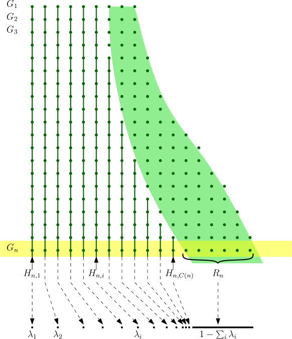
Figure 3.7. Illustration of the Comb structure theorem

We shall now extend the Comb structure theorem to full ${\rm FO}$-convergence. In contrast with the case of a finite $\varpi$-spectrum, the elementary convergence aspects will be non trivial and will require a careful choice of a clip for the sequence.

Lemma 3.65.

Let $(\mathbf{A}_{n})_{n\in\mathbb{N}}$ be an ${\rm FO}^{\rm local}$-convergent sequence of finite $\lambda$-structures with component relation $\varpi$, such that $\lim_{n\rightarrow\infty}|A_{n}|=\infty$. Let $\mathbf{B}_{n,i}$ be the connected components of $\mathbf{A}_{n}$. Assume that the connected components with same $\hskip 1.0pt\mathsf{sp}_{i}$ have been reshuffled according to Lemma 3.56, so that $(\mathbf{B}_{n,i})_{i\in\mathbb{N}}$ is ${\rm FO}$-convergent for each $i\in\mathbb{N}$.

For $i\in\mathbb{N}$, let $\widehat{\mathbf{B}_{i}}$ be an elementary limit of $(\mathbf{B}_{n,i})_{n\in\mathbb{N}}$. Then there exists a clip $C$ such that the sequence $(\mathbf{R}_{n})_{n\in\mathbb{N}}$ of the residues is elementarily convergent. Moreover, if $\widehat{\mathbf{R}}$ is an elementary limit of $(\mathbf{R}_{n})_{n\in\mathbb{N}}$, then $\bigcup_{i}\widehat{\mathbf{B}_{i}}\cup\widehat{\mathbf{R}}$ is an elementary limit of $(\mathbf{A}_{n})_{n\in\mathbb{N}}$.

Let $\mathbf{B}_{n,i}^{\prime}$ be either $\mathbf{B}_{n,i}$ if $C(n)\geq i$ or the empty $\lambda$-structure if $C(n)<i$. Then the family consisting in the sequences $(\mathbf{B}_{n,i}^{\prime})_{i\in\mathbb{N}}$ ($i\in\mathbb{N}$) and of the sequence $(\mathbf{R}_{n})_{n\in\mathbb{N}}$ is uniformly elementarily convergent.

Proof.

Let $\widehat{\mathbf{A}}$ be an elementary limit of $(\mathbf{A}_{n})_{n\in\mathbb{N}}$.

For $\theta\in{\rm FO}_{1}^{\rm local}$ and $m\in\mathbb{N}$ we denote by $\theta^{(m)}$ the sentence

$$\theta^{(m)}:\quad(\exists x_{1}\dots\exists x_{m})\ \biggl{(}\bigwedge_{1\leq i<j\leq m}\neg\varpi(x_{i},x_{j})\ \wedge\ \bigwedge_{i=1}^{m}\theta(x_{i})\biggr{)}.$$

According to Theorem 2.21, elementary convergence of a sequence of $\lambda$-structures with component relation $\varpi$ can be checked by considering sentences of the form $\theta^{(k)}$ for $\theta\in{\rm FO}_{1}^{\rm local}$ and $k\in\mathbb{N}$.

Note that for every $k<k^{\prime}$ and every $\lambda$-structure $\mathbf{A}$, if it holds that $\mathbf{A}\models\theta^{(k^{\prime})}$ then it holds that $\mathbf{A}\models\theta^{(k)}$. Define

$$M(\theta) =\sup\{k\in\mathbb{N}:\quad\widehat{\mathbf{A}}\models\theta^{(k)}\}$$

$$\Omega(\theta) =\{i\in\mathbb{N}:\quad\widehat{\mathbf{B}_{i}}\models(\exists x)\theta(x)\}.$$

Note that obviously $|\Omega(\theta)|\leq M(\theta)$.

For $r\in\mathbb{N}$, let $\theta_{1},\dots,\theta_{F(r)}$ be an enumeration of the local first-order formulas with a single free variable with quantifier rank at most $r$ (up to logical equivalence). Define

$$A(r)=\max(r,\max_{a\leq F(r)}\max\Omega(\theta_{a})).$$

Let

$$C_{0}(n)=\sup\biggl{\{}K\in\mathbb{N}:\quad(\forall n^{\prime}\geq n)\ \sum_{i=1}^{K}\biggl{|}\frac{|B_{n^{\prime},i}|}{|A_{n^{\prime}}|}-\hskip 1.0pt\mathsf{sp}_{i}\biggr{|}\leq\sum_{i>K}\hskip 1.0pt\mathsf{sp}_{i}\biggr{\}}$$

be the standard (maximal) clip on $(\mathbf{A}_{n})_{n\in\mathbb{N}}$ (see Proposition 3.61).

Let $B(r)$ be the minimum integer such that

1. it holds that $C_{0}(B(r))\geq A(r)$ (note that $\lim_{n\rightarrow\infty}C_{0}(n)=\infty$, according to Proposition 3.61);

2. for every $n\geq B(r),a\leq F(r)$ and every $k\leq r$ it holds that $\mathbf{A}_{n}\models\theta_{a}^{(k)}$ if and only if $M(\theta_{a})\geq k$ (note that this holds for sufficiently large $n$ as $\widehat{\mathbf{A}}$ is an elementary limit of $(\mathbf{A}_{n})_{n\in\mathbb{N}}$);

3. for every $i\leq A(r)$ and $a\leq F(r)$ the following equivalence holds:

   $$\mathbf{B}_{n,i}\models(\exists x)\theta_{a}(x)\quad\iff\quad\widehat{\mathbf{B}_{i}}\models(\exists x)\theta_{a}(x).$$

   (note that this holds for sufficiently large $n$ as $\widehat{\mathbf{B}_{i}}$ is an elementary limit of $(\mathbf{B}_{n,i})_{n\in\mathbb{N}}$ and as we consider only finitely many values of $i$);

we define the non-decreasing function $C:\mathbb{N}\rightarrow\mathbb{N}$ by

$$C(n)=\max\{A(r):B(r)\leq n\}.$$

As $\lim_{r\rightarrow\infty}A(r)=\infty$ and as $C_{0}(B(r))\geq A(r)$ it holds that $\lim_{r\rightarrow\infty}B(r)=\infty$. Moreover, for every $r\in\mathbb{N}$ it holds that $C_{0}(B(r))\geq A(r)$ hence $C_{0}(n)\geq C(n)$. According to Proposition 3.61, it follows that the function $C$ is a clip on $(\mathbf{A}_{n})_{n\in\mathbb{N}}$.

Let $(\mathbf{R}_{n})_{n\in\mathbb{N}}$ be the residue of $(\mathbf{A}_{n})_{n\in\mathbb{N}}$ with respect to the clip $C$, and let $\mathbf{B}_{n,i}^{\prime}$ be defined as $\mathbf{B}_{n,i}$ if $i\leq C(n)$ and the empty $\lambda$-structure otherwise. Then it is immediate from the definition of the clip $C$ that the family $\{(B_{n,i}^{\prime})_{n\in\mathbb{N}}:\ i\in\mathbb{N}\}$ is uniformly elementarily convergent. Using Lemma 3.23, it is also easily checked that the residue $(\mathbf{R}_{n})_{n\in\mathbb{N}}$ of $(\mathbf{A}_{n})_{n\in\mathbb{N}}$ with respect to the clip $C$ is elementarily convergent and thus, that the family $\{(B_{n,i}^{\prime})_{n\in\mathbb{N}}:\ i\in\mathbb{N}\}\cup\{(\mathbf{R}_{n})_{n\in\mathbb{N}}\}$ is uniformly elementarily convergent. ∎

The extension of the Comb structure theorem to ${\rm FO}$-convergence now follows directly.

Theorem 3.66 (Comb structure for $\lambda$-structure sequences with infinite spectrum).

Let $(\mathbf{A}_{n})_{n\in\mathbb{N}}$ be an ${\rm FO}$-convergent sequence of finite $\lambda$-structures with component relation $\varpi$ and infinite spectrum $(\hskip 1.0pt\mathsf{sp}_{i})_{i\in\mathbb{N}}$.

Then there exists a clip $C:\mathbb{N}\rightarrow\mathbb{N}$ with residue $\mathbf{R}_{n}$ and, for each $n\in\mathbb{N}$, a permutation $f_{n}:[C(n)]\rightarrow[C(n)]$ such that, extending $f_{n}$ to $\mathbb{N}$ by putting $f(i)$ to be the identity for $i>C(n)$, and letting $\mathbf{B}_{n,i}^{\prime}$ be either $\mathbf{B}_{n,f_{n}(i)}$ if $C(n)\geq i$ or the empty $\lambda$-structure if $C(n)<i$, the following holds:

• $\mathbf{A}_{n}=\mathbf{R}_{n}\cup\bigcup_{i\in\mathbb{N}}\mathbf{B}_{n,i}^{\prime}$;

• $\lim_{n\rightarrow\infty}\max_{i>C(n)}|B_{n,i}^{\prime}|/|A_{n}|=0$;

• $\lim_{n\rightarrow\infty}|R_{n}|/|A_{n}|$ exists;

• for every $i\in\mathbb{N}$, $(\mathbf{B}_{n,i}^{\prime})_{n\in\mathbb{N}}$ is ${\rm FO}$-convergent;

• either $\lim_{n\rightarrow\infty}|R_{n}|/|A_{n}|=0$ and $(\mathbf{R}_{n})_{n\in\mathbb{N}}$ is elementarily convergent, or the sequence $(\mathbf{R}_{n})_{n\in\mathbb{N}}$ is ${\rm FO}$-convergent;

• the family $\{(\mathbf{B}_{n,i}^{\prime})_{n\in\mathbb{N}}:i\in\mathbb{N}\}\cup\{(\mathbf{R}_{n})_{n\in\mathbb{N}}\}$ is uniformly elementarily convergent.

This ends the (admittedly very technical and complicated) analysis of the component structure of limits. This was not developed for its own sake, but it will be all needed in the Part 3 of this paper, to construct modeling ${\rm FO}$-limits for convergent sequences of trees with bounded height and, by means of a fitting basic interpretation scheme, to graphs with bounded tree-depth (defined in [68]), or graphs with bounded SC-depth (defined in [41]).

In a broader sense, this detailed analysis was a cradle of much of the further research (see Addendum Section 5.2).

Chapter 4 Limits of Graphs with Bounded Tree-depth

In this part, we mainly consider the signature $\lambda$, which consists in a binary relation $\sim$ (symmetric adjacency relation), a unary relation $R$ (property of being a root), and $c$ unary relations $C_{i}$ (the coloring). Colored rooted trees with height at most $h$ are particular $\lambda$-structures, and the class of (finite or infinite) colored rooted trees with height at most $h$ will be denoted by $\mathcal{Y}^{(h)}$. (Here we shall be only concerned with trees that are either finite, countable, or of size continuum.)

4.1. ${\rm FO}_{1}$-limits of Colored Rooted Trees with Bounded Height

In this section, we explicitly define modeling ${\rm FO}_{1}$-limits for ${\rm FO}_{1}$-convergent sequences of colored rooted trees with bounded height and characterize modelings which are ${\rm FO}_{1}$-limits for ${\rm FO}_{1}$-convergent sequences of (finite) colored rooted trees with bounded height.

4.1.1. Preliminary Observations

We take some time for some preliminary observations on the logical structure of rooted colored trees with bounded height. These observations will use arguments based on Ehrenfeucht-Fraïssé games and strategy stealing. (For definitions of $\equiv^{n}$ and Ehrenfeucht-Fraïssé games, see Section 2.3.1.)

For a rooted colored tree $\mathbf{Y}\in\mathcal{Y}^{(h)}$ and a vertex $x\in Y$, we denote by $\mathbf{Y}(x)$ the subtree of $\mathbf{Y}$ rooted at $x$ — that is the subtree of $\mathbf{Y}$ with root $x$ induced by $x$ and all its descendants — and (for a non-root $x$) by $\mathbf{Y}\setminus\mathbf{Y}(x)$ the rooted tree obtained from $\mathbf{Y}$ by removing all the vertices in $\mathbf{Y}(x)$.

The following two lemmas show that, like for isomorphism, equivalence between two colored rooted trees can be reduced to equivalence of branches.

Lemma 4.1.

Let $\mathbf{Y},\mathbf{Y}^{\prime}\in\mathcal{Y}^{(h)}$, let $s,s^{\prime}$ be sons of the roots of $\mathbf{Y}$ and $\mathbf{Y}^{\prime}$, respectively.

Let $n\in\mathbb{N}$. If $\mathbf{Y}(s)\equiv^{n}\mathbf{Y}^{\prime}(s^{\prime})$ and $\mathbf{Y}\setminus\mathbf{Y}(s)\equiv^{n}\mathbf{Y}^{\prime}\setminus\mathbf{Y}^{\prime}(s^{\prime})$, then $\mathbf{Y}\equiv^{n}\mathbf{Y}^{\prime}$.

Proof.

Assume $\mathbf{Y}(s)\equiv^{n}\mathbf{Y}^{\prime}(s^{\prime})$ and $\mathbf{Y}\setminus\mathbf{Y}(s)\equiv^{n}\mathbf{Y}^{\prime}\setminus\mathbf{Y}^{\prime}(s^{\prime})$. In order to prove $\mathbf{Y}\equiv^{n}\mathbf{Y}^{\prime}$ we play an $n$-step Ehrenfeucht-Fraïssé-game ${\rm EF}_{0}$ on $\mathbf{Y}$ and $\mathbf{Y}^{\prime}$ as Duplicator. Our strategy will be based on two auxiliary $n$-step Ehrenfeucht-Fraïssé-games, ${\rm EF}_{1}$ and ${\rm EF}_{2}$, on $\mathbf{Y}(s)$ and $\mathbf{Y}^{\prime}(s^{\prime})$ and on $\mathbf{Y}\setminus\mathbf{Y}(s)$ and $\mathbf{Y}^{\prime}\setminus\mathbf{Y}^{\prime}(s^{\prime})$, respectively, against Duplicators following a winning strategy. Each time Spoiler selects a vertex in game ${\rm EF}_{0}$, we play the same vertex in the game ${\rm EF}_{1}$ or ${\rm EF}_{2}$ (depending on the tree the vertex belongs to), then we mimic the selection of the Duplicator of this game. It is easily checked that this strategy is a winning strategy. ∎

Lemma 4.2.

Let $\mathbf{Y},\mathbf{Y}^{\prime}\in\mathcal{Y}^{(h)}$, let $s,s^{\prime}$ be sons of the roots of $\mathbf{Y}$ and $\mathbf{Y}^{\prime}$, respectively.

Let $n\in\mathbb{N}$. If $\mathbf{Y}\equiv^{n+h}\mathbf{Y}^{\prime}$ and $\mathbf{Y}(s)\equiv^{n}\mathbf{Y}^{\prime}(s^{\prime})$, then $\mathbf{Y}\setminus\mathbf{Y}(s)\equiv^{n}\mathbf{Y}^{\prime}\setminus\mathbf{Y}^{\prime}(s^{\prime})$.

Proof.

Assume $\mathbf{Y}\equiv^{n+h}\mathbf{Y}^{\prime}$ and $\mathbf{Y}(s)\equiv^{n}\mathbf{Y}^{\prime}(s^{\prime})$.

We first play (as Spoiler) $s$ in $\mathbf{Y}$ then $s^{\prime}$ in $\mathbf{Y}^{\prime}$. Let $t^{\prime}$ and $t$ be the corresponding plays of Duplicator. Then the further $n$ steps of the game have to map vertices in $\mathbf{Y}(s)$, $\mathbf{Y}(t)$, $\mathbf{Y}\setminus(\mathbf{Y}(s)\cup\mathbf{Y}(t))$ to $\mathbf{Y}^{\prime}(t^{\prime})$, $\mathbf{Y}^{\prime}(s^{\prime})$, $\mathbf{Y}^{\prime}\setminus(\mathbf{Y}^{\prime}(t^{\prime})\cup\mathbf{Y}^{\prime}(s^{\prime}))$ (and converse), for otherwise $h-2$ steps would allow Spoiler to win the game. Also, by restricting our play to one of these pairs of trees, we deduce $\mathbf{Y}(s)\equiv^{n}\mathbf{Y}^{\prime}(t^{\prime})$, $\mathbf{Y}(t)\equiv^{n}\mathbf{Y}^{\prime}(s^{\prime})$, and $\mathbf{Y}\setminus(\mathbf{Y}(s)\cup\mathbf{Y}(t))\equiv^{n}\mathbf{Y}\setminus(\mathbf{Y}^{\prime}(s^{\prime})\cup\mathbf{Y}^{\prime}(t^{\prime}))$. As $\mathbf{Y}^{\prime}(s^{\prime})\equiv^{n}\mathbf{Y}(s)$ it follows

$$\mathbf{Y}(t)\equiv^{n}\mathbf{Y}^{\prime}(s^{\prime})\equiv^{n}\mathbf{Y}(s)\equiv^{n}\mathbf{Y}^{\prime}(t^{\prime}).$$

Hence, according to Lemma 4.1, as $\mathbf{Y}\setminus(\mathbf{Y}(s)\cup\mathbf{Y}(t))=(\mathbf{Y}\setminus\mathbf{Y}(s))\setminus\mathbf{Y}(t)$ and $\mathbf{Y}^{\prime}\setminus(\mathbf{Y}^{\prime}(s^{\prime})\cup\mathbf{Y}^{\prime}(t^{\prime}))=(\mathbf{Y}^{\prime}\setminus\mathbf{Y}^{\prime}(s^{\prime}))\setminus\mathbf{Y}^{\prime}(t^{\prime})$, we deduce $\mathbf{Y}\setminus\mathbf{Y}(s)\equiv^{n}\mathbf{Y}^{\prime}\setminus\mathbf{Y}^{\prime}(s^{\prime})$. ∎

Let $\lambda^{\bullet}$ denote the signature obtained from $\lambda$ by adding a new unary relation $S$ (marking a special vertex, which is not necessarily the root). Let $\theta_{\bullet}$ be the sentence

$$(\exists x)(S(x)\wedge(\forall y\ S(y)\rightarrow(y=x))),$$

which states that a $\lambda^{\bullet}$ contains a unique special vertex. We denote by $\mathcal{Y}^{(h)}_{\bullet}$ the class obtained by marking as special a single vertex of a colored rooted tree with height at most $h$. Let ${\rm Unmark}$ be the interpretation of $\lambda$-structures in $\lambda^{\bullet}$-structures consisting in forgetting $S$ (so that ${\rm Unmark}$ projects $\mathcal{Y}^{(h)}_{\bullet}$ onto $\mathcal{Y}^{(h)}$).

Lemma 4.3.

Let $\mathbf{Y},\mathbf{Y}^{\prime}\in\mathcal{Y}^{(h)}_{\bullet}$ be such that $\mathbf{Y}$ (resp. $\mathbf{Y}^{\prime}$) has special vertex $m$ (resp. $m^{\prime}$). Assume that both $m$ and $m^{\prime}$ have height $t>1$ (in $\mathbf{Y}$ and $\mathbf{Y}^{\prime}$, respectively). Let $v$ (resp. $v^{\prime}$) be son of the root of $\mathbf{Y}$ (resp. $\mathbf{Y}^{\prime}$) that is an ancestor of $m$ (resp. $m^{\prime}$).

Then for every $n\in\mathbb{N}$, if ${\rm Unmark}(\mathbf{Y})\equiv^{n+h}{\rm Unmark}(\mathbf{Y}^{\prime})$ and $\mathbf{Y}(v)\equiv^{n}\mathbf{Y}^{\prime}(v^{\prime})$, then $\mathbf{Y}\equiv^{n}\mathbf{Y}^{\prime}$.

Proof.

Assume ${\rm Unmark}(\mathbf{Y})\equiv^{n+h}{\rm Unmark}(\mathbf{Y}^{\prime})$ and $\mathbf{Y}(v)\equiv^{n}\mathbf{Y}^{\prime}(v^{\prime})$. Then it holds that ${\rm Unmark}(\mathbf{Y}(v))\equiv^{n}{\rm Unmark}(\mathbf{Y}^{\prime}(v^{\prime}))$ thus, according to Lemma 4.2,

$$\mathbf{Y}\setminus\mathbf{Y}(v) ={\rm Unmark}(\mathbf{Y})\setminus{\rm Unmark}(\mathbf{Y}(v))$$

$$\equiv^{n}{\rm Unmark}(\mathbf{Y}^{\prime})\setminus{\rm Unmark}(\mathbf{Y}^{\prime}(v^{\prime}))=\mathbf{Y}^{\prime}\setminus\mathbf{Y}^{\prime}(v^{\prime}).$$

Hence, according to Lemma 4.1, it holds that $\mathbf{Y}\equiv^{n}\mathbf{Y}^{\prime}$ (as the marking could be considered as a coloring). ∎

The next lemma states that the properties of a colored rooted trees with a distinguished vertex $v$ (which is not necessarily the root) can be retrieved from the properties of the subtree rooted at $v$, the subtree rooted at the father of $v$, etc. (see Fig. 4.1).

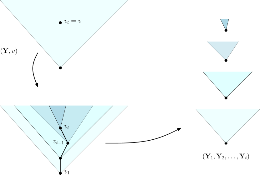
Figure 4.1. Transformation of a rooted tree with a distinguished vertex $(\mathbf{Y},v_{t})$ into a tuple of rooted trees $(\mathbf{Y}_{1},\dots,\mathbf{Y}_{t})$.

Lemma 4.4.

Let $\mathbf{Y},\mathbf{Y}^{\prime}\in\mathcal{Y}^{(h)}$, $v_{t}\in Y$ and $v_{t}^{\prime}\in Y^{\prime}$ be vertices with height $t$. For $1\leq i<t$, let $v_{i}$ (resp. $v_{i}^{\prime}$) be the ancestor of $v_{t}$ (resp. of $v_{t}^{\prime}$) at height $i$.

Then for every integer $n$ it holds that

$$(\forall 1\leq i\leq t)\ \mathbf{Y}(v_{i})\equiv^{n+h+1-i}\mathbf{Y}^{\prime}(v_{i}^{\prime})\ \Longrightarrow\ (\mathbf{Y},v_{t})\equiv^{n}(\mathbf{Y}^{\prime},v_{t}^{\prime})$$

$$(\mathbf{Y},v_{t})\equiv^{n+(t-1)h}(\mathbf{Y}^{\prime},v_{t}^{\prime})\ \Longrightarrow\ (\forall 1\leq i\leq t)\ \mathbf{Y}(v_{i})\equiv^{n+(t-i)h}\mathbf{Y}^{\prime}(v_{i}^{\prime})$$

Proof.

We proceed by induction over $t$. If $t=1$, then the statement obviously holds. So, assume $t>1$ and that the statement holds for $t-1$.

Let $\mathbf{Y}_{\bullet},\mathbf{Y}_{\bullet}^{\prime}\in\mathcal{Y}^{(h)}_{\bullet}$ be the marked rooted colored trees obtained from $\mathbf{Y}$ and $\mathbf{Y}^{\prime}$ by marking $v_{t}$ (resp. $v_{t}^{\prime}$) as a special vertex.

Assume $(\forall 1\leq i\leq t)\ \mathbf{Y}(v_{i})\equiv^{n+h+1-i}\mathbf{Y}^{\prime}(v_{i}^{\prime})$. By induction, $(\forall 2\leq i\leq t)\ \mathbf{Y}(v_{i})\equiv^{n+(h-1)+1-(i-1)}\mathbf{Y}^{\prime}(v_{i}^{\prime})$ implies $(\mathbf{Y}(v_{2}),v_{t})\equiv^{n}(\mathbf{Y}^{\prime}(v_{2}^{\prime}),v_{t}^{\prime})$, that is $\mathbf{Y}_{\bullet}(v_{2})\equiv^{n}\mathbf{Y}_{\bullet}^{\prime}(v_{2}^{\prime})$. As $\mathbf{Y}\equiv^{n+h}\mathbf{Y}^{\prime}$, it follows from Lemma 4.3 that $\mathbf{Y}_{\bullet}\equiv^{n}\mathbf{Y}_{\bullet}^{\prime}$, that is: $(\mathbf{Y},v_{t})\equiv^{n}(\mathbf{Y}^{\prime},v_{t}^{\prime})$.

Conversely, if $(\mathbf{Y},v_{t})\equiv^{n+(t-1)h}(\mathbf{Y}^{\prime},v_{t}^{\prime})$ (i.e. $\mathbf{Y}_{\bullet}\equiv^{n+(t-1)h}\mathbf{Y}_{\bullet}^{\prime}$) an repeated application of Lemma 4.2 gives $\mathbf{Y}_{\bullet}(v_{i})\equiv^{n+(t-i)h}\mathbf{Y}_{\bullet}^{\prime}(v_{i})^{\prime}$ hence (by forgetting the marking) $\mathbf{Y}(v_{i})\equiv^{n+(t-i)h}\mathbf{Y}^{\prime}(v_{i})^{\prime}$. ∎

This lemma allows to encode the complete theory of a colored rooted tree $\mathbf{Y}$ of height at most $h$ with special vertex $v$ as a tuple of complete theories of colored rooted trees with height at most $h$.

In fact what follows could be described as a fine analysis of the Stone dual of the Boolean algebra of all the formulas having a model in $\mathcal{Y}^{(h)}$. As the height $h$ is bounded, the classes $\mathcal{Y}^{(h)}$ can be axiomatized by finitely many axioms (hence by some single axiom $\eta_{\mathcal{Y}^{(h)}}$), it is a basic elementary class. For an integer $p\geq 0$, we introduce a short notation for the Stone space associated to the Lindenbaum–Tarski algebra of formulas on $\mathcal{Y}^{(h)}$ with $p$ free variables:

$$\mathfrak{Y}_{p}^{(h)}=S(\mathcal{B}({\rm FO}_{p}(\lambda),\eta_{\mathcal{Y}^{(h)}})).$$

We shall now move from models to theories, specifically from $\mathcal{Y}_{\bullet}^{(h)}$ (colored rooted trees with height at most $h$ and a special vertex) to the Stone space $\mathfrak{Y}_{1}^{(h)}$ and from $\mathcal{Y}^{(h)}$ (colored rooted trees with height at most $h$) to the Stone space $\mathfrak{Y}_{0}^{(h)}$.

In that direction, we first show how the notion of “property of the subtree $\mathbf{Y}(v)$ of $\mathbf{Y}$ rooted at the vertex $v$” translates into a relativization homomorphism $\varrho:\mathcal{B}({\rm FO}_{0}(\lambda))\rightarrow\mathcal{B}({\rm FO}_{1}(\lambda))$.

We consider the simple interpretation ${\mathsf{I}}_{\bullet}$ of $\lambda$-structures in $\lambda^{\bullet}$-structures, which maps a $\lambda^{\bullet}$-structure $\mathbf{Y}_{\bullet}$ to the $\lambda$-structure defined as follows: let $x\simeq y$ be defined as $(x\sim y)\vee(x=y)$. Then

• the domain of ${\mathsf{I}}_{\bullet}(\mathbf{Y}_{\bullet})$ is defined by the formula

  $$S(x_{1})\vee(\forall y_{1},\dots,y_{h})\Bigl{(}\bigl{(}R(y_{1})\wedge\bigwedge_{i=1}^{h-1}\neg S(y_{i})\wedge(y_{i}\simeq y_{i+1})\bigr{)}\rightarrow(y_{h}\neq x_{1})\Bigr{)};$$

• the adjacency relation $\sim$ is defined as in $\mathbf{Y}_{\bullet}$ (i.e. by the formula $(x_{1}\sim x_{2})$);

• the relation $R$ of ${\mathsf{I}}_{\bullet}(\mathbf{Y}_{\bullet})$ is defined by the formula $S(x_{1})$.

Although ${\mathsf{I}}_{\bullet}$ maps general $\lambda_{\bullet}$-structures to $\lambda$-structures, we shall be only concerned by the specific property that ${\mathsf{I}}_{\bullet}$ maps a rooted tree $\mathbf{Y}_{\bullet}\in{\mathcal{Y}}^{(h)}_{\bullet}$ with special vertex $v$ to the rooted tree ${\rm Unmark}(\mathbf{Y}_{\bullet})(v)$.

In a sake for simplicity, for $\mathbf{Y}\in{\mathcal{Y}}^{(h)}$ we denote by $(\mathbf{Y},v)$ (where $\mathbf{Y}$ is a $\lambda$-structure) the $\lambda^{\bullet}$-structure obtained by adding the new relation $S$ with $v$ being the unique special vertex.

Lemma 4.5.

There is a Boolean algebra homomorphism

$$\varrho:\mathcal{B}({\rm FO}_{0}(\lambda),\eta_{\mathcal{Y}^{(h)}})\rightarrow\mathcal{B}({\rm FO}_{1}(\lambda),\eta_{\mathcal{Y}^{(h)}})$$

(called relativization), such that for every sentence $\phi\in{\rm FO}_{0}(\lambda)$, every $\mathbf{Y}\in\mathcal{Y}^{(h)}$, and every $v\in Y$ the following equivalence holds

$$\mathbf{Y}(u)\models\phi\quad\iff\quad\mathbf{Y}\models\varrho(\phi)(u).$$

Proof.

The lemma follows from the property

$$\mathbf{Y}(u)\models\phi\quad\iff\quad{\mathsf{I}}_{\bullet}(\mathbf{Y},u)\models\phi\quad\iff\quad(\mathbf{Y},u)\models{\tilde{\mathsf{I}}}_{\bullet}(\phi).$$

The formula $\rho(\phi)$ is obtained from the sentence ${\tilde{\mathsf{I}}}_{\bullet}(\phi)$ by replacing each occurrence of $S(y)$ by $y=x_{1}$. ∎

Using relativization and Lemma 4.4, we can translate the transformation shown on Figure 4.1 to a encoding of elements of $\mathfrak{Y}_{1}^{(h)}$ into tuples of elements $\mathfrak{Y}_{0}^{(h)}$. Intuitively, a element $T\in\mathfrak{Y}_{1}^{(h)}$ defines the properties of a colored rooted tree $\mathbf{Y}$ with special vertex $x_{1}$, and the relativization $\rho$ allows us to extract from $T$ the tuple of the complete theories of the subtrees of $\mathbf{Y}$ rooted at $x_{1}$, the father of $x_{1}$, etc.  Moreover, the meaning of Lemma 4.4 is that what we obtain only depends on the complete theory of $(\mathbf{Y},x_{1})$, that is only on $T$.

Definition 4.6.

For $1\leq i\leq h$, let $\eta_{i}\in{\rm FO}_{1}(\lambda)$ be the formula stating that the height of $x_{1}$ is $i$.

We define the mapping ${\rm Encode}:\mathfrak{Y}_{1}^{(h)}\rightarrow\biguplus_{k=1}^{h}(\mathfrak{Y}_{0}^{(h)})^{k}$ as follows:

For $T\in\mathfrak{Y}_{1}^{(h)}$, let $k$ be the (unique) integer such that $\eta_{k}\in T$. Then ${\rm Encode}(T)$ is the $k$-tuple $(T_{0},\dots,T_{k-1})$, where

• $T_{k-1}$ is the set of sentences $\theta\in{\rm FO}_{0}(\lambda)$ such that $\rho(\theta)\in T$ (intuitively, the complete theory of the subtree rooted at $x_{1}$);

• $T_{k-2}$ is the set of sentences $\theta\in{\rm FO}_{0}(\lambda)$ such that

  $$\bigl{(}(\exists y_{1})(\eta_{k-1}(y_{1})\wedge y_{1}\sim x_{1}\wedge\rho(\theta)(y))\bigr{)}\in T$$

  (intuitively, the complete theory of the subtree rooted at the father of $x_{1}$);

• $T_{k-1-i}$ is the set of sentences $\theta\in{\rm FO}_{0}(\lambda)$ such that

  $$\bigl{(}(\exists y_{1}\dots y_{i})(\bigwedge_{j=1}^{i}\eta_{k-j}(y_{j})\wedge\bigwedge_{j=1}^{i-1}(y_{j}\sim y_{j+1}\wedge y_{1}\sim x_{1}\wedge\rho(\theta)(y_{i})\bigr{)}\in T$$

  (intuitively, the complete theory of the subtree rooted at the ancestor of $x_{1}$ which has height $k-i$);

• $T_{0}=T\cap\in{\rm FO}_{0}(\lambda)$ (intuitively, the complete theory of the whole rooted tree).

Lemma 4.7.

${\rm Encode}$ is a homeomorphism of $\mathfrak{Y}_{1}^{(h)}$ and ${\rm Encode}(\mathfrak{Y}_{1}^{(h)})$, which is a closed subspace of $\biguplus_{k=1}^{h}(\mathfrak{Y}_{0}^{(h)})^{k}$.

Proof.

This lemma is a direct consequence of Lemma 4.4. ∎

4.1.2. The Universal Relational Sample Space $\mathbb{Y}_{h}$

The aim of this section is to construct a rooted colored forest on a standard Borel space $\mathbb{Y}_{h}$ that is ${\rm FO}_{1}$-universal, in the sense that every ${\rm FO}_{1}$-convergent sequence of colored rooted trees will have a modeling ${\rm FO}_{1}$-limit obtained by assigning an adapted probability measure to one of the connected components of $\mathbb{Y}_{h}$.

Definition 4.8.

For theories $T,T^{\prime}\in\mathfrak{Y}_{0}^{(h)}$, we define $w(T,T^{\prime})\geq k$ if and only if there exists a model $\mathbf{Y}$ of $T$, such that the root of $\mathbf{Y}$ has $k$ (distinct) sons $v_{1},\dots,v_{k}$ with ${\rm Th}(\mathbf{Y}(v_{i}))=T^{\prime}$.

Lemma 4.9.

For $k\in\mathbb{N}$ and $\phi\in{\rm FO}_{0}$, let $\zeta_{k}(\phi)$ be the sentence $(\exists^{\geq k}y)\ \rho(\phi)(y)$. Then $w(T,T^{\prime})\geq k$ if and only if $\zeta_{k}(\phi)\in T$ holds for every $\phi\in T^{\prime}$.

Proof.

If $w(T,T^{\prime})\geq k$, then $\zeta_{k}(\phi)\in T$ holds for every $\phi\in T^{\prime}$, hence we only have to prove the opposite direction. Assume that $\zeta_{k}(\phi)\in T$ holds for every $\phi\in T^{\prime}$, but that there is $\phi_{0}\in T^{\prime}$ such that $\zeta_{k+1}(\phi_{0})\notin T$. Let $Y$ be a model of $T$, and let $v_{1},\dots,v_{k}$ be the sons of the root of $Y$ such that $Y(v_{i})\models\phi_{0}$. For every $r\in\mathbb{N}$, $r\geq{\rm qrank}(\phi_{0})$, let $\psi_{r}$ be the conjunction of the sentences in $T^{\prime}$ with quantifier rank $r$. Obviously, $\psi_{r}\in T^{\prime}$. Moreover, as $\zeta_{k}(\psi_{r})\in T$, it holds that $Y\models\zeta_{k}(\psi_{r})$. As $\psi_{r}\vdash\phi_{0}$, it follows that for every $1\leq i\leq k$ it holds that $Y(v_{i})\models\psi_{r}$ (only possible choices). As this holds for every $r$, we infer that for every $1\leq i\leq k$, $Y(v_{i})$ is a model of $T^{\prime}$ hence $w(T,T^{\prime})\geq k$. Now assume that for every $k\in\mathbb{N}$ and every $\phi\in T^{\prime}$ it holds that $\zeta_{k}(\phi)\in T$. Let $Y$ be a model of $T$, let $Y^{\prime}$ be a model of $T^{\prime}$, and let $\tilde{Y}$ be obtained from $Y$ by adding (at the root of $Y$) a son $u$ with subtree $\tilde{Y}(u)$ isomorphic to $Y^{\prime}$. By an easy application of an Ehrenfeucht-Fraïssé game, we get that $\tilde{Y}$ is elementarily equivalent to $Y$, hence a model of $T$. Thus $w(T,T^{\prime})\geq k$. ∎

Let $\overline{\mathbb{N}}$ be the one point compactification of $\mathbb{N}$, that is $\overline{\mathbb{N}}=\mathbb{N}\cup\{\infty\}$ with open sets generated by complements of finite sets.

Lemma 4.10.

The function $w:\mathfrak{Y}_{0}^{(h)}\times\mathfrak{Y}_{0}^{(h)}\rightarrow\overline{\mathbb{N}}$ is upper semicontinuous (with respect to product topology of Stone space $\mathfrak{Y}_{0}^{(h)}$).

Proof.

For $r\in\mathbb{N}$ define the function $w_{r}:\mathfrak{Y}_{0}^{(h)}\times\mathfrak{Y}_{0}^{(h)}\rightarrow\overline{\mathbb{N}}$ by:

$$w_{r}(T,T^{\prime})=\sup\{k\in\mathbb{N}:\ \forall\psi\in T^{\prime}\ ({\rm qrank}(\psi)\leq r)\Rightarrow\zeta_{k}(\psi)\in T\}.$$

It follows from Lemma 4.9 that the following equation holds

$$w(T,T^{\prime})=\inf_{r\in\mathbb{N}}w_{r}(T,T^{\prime}).$$

Hence, in order to prove that the function $w$ is upper semicontinuous, it is sufficient to prove that the functions $w_{r}$ are continuous. Let $(T_{0},T_{0}^{\prime})\in\mathfrak{Y}_{0}^{(h)}\times\mathfrak{Y}_{0}^{(h)}$. We distinguish two cases:

– Firstly, assume $w_{r}(T_{0},T_{0}^{\prime})=k$.

If ${\rm dist}(T^{\prime},T_{0}^{\prime})<2^{-r}$ and ${\rm dist}(T,T_{0})<2^{-\max\{{\rm qrank}(\zeta_{k+1}(\psi)):\ {\rm qrank}(\psi)\leq r\}}$, then it holds that $w_{r}(T,T^{\prime})=w_{r}(T_{0},T_{0}^{\prime})$;

– Secondly, assume $w_{r}(T_{0},T_{0}^{\prime})=\infty$, and let $k\in\mathbb{N}$.

If ${\rm dist}(T^{\prime},T_{0}^{\prime})<2^{-r}$ and ${\rm dist}(T,T_{0})<2^{-\max\{{\rm qrank}(\zeta_{k+1}(\psi)):\ {\rm qrank}(\psi)\leq r\}}$, then it holds that $w_{r}(T,T^{\prime})>k$. ∎

For $z=(z_{1},\dots,z_{a})\in\overline{\mathbb{N}}^{a}$ define the subset $F_{z}$ of $(\mathfrak{Y}_{0}^{(h)})^{a+1}$ by

$$F_{z}=\{(T_{0},\dots,T_{a}):w(T_{i-1},T_{i})=z_{i}\}.$$

For $t\in\overline{\mathbb{N}}$, define

$$X_{t}=\begin{cases}\{1,\dots,t\},&\text{if }t\in\mathbb{N},\\ [0,1],&\text{if }t=\infty.\end{cases}$$

For $z=(z_{1},\dots,z_{a})\in\overline{\mathbb{N}}^{a}$, define $X_{z}=\prod_{i=1}^{a}X_{z_{i}}$. Let

$$V_{h}=\mathfrak{Y}_{0}^{(h)}\uplus\biguplus_{a=1}^{h-1}\biguplus_{z\in\overline{\mathbb{N}}^{a}}(F_{z}\times X_{z}).$$

Definition 4.11.

The universal forest $\mathbb{Y}_{h}$ has vertex set $V_{h}$. The roots of $\mathbb{Y}_{h}$ are the elements in $\mathfrak{Y}_{0}^{(h)}$. The edges of $\mathbb{Y}_{h}$ are the pairs of the form

$$\{((T_{0},T_{1},\dots,T_{a}),(\alpha_{1},\dots,\alpha_{a})),((T_{0},T_{1},\dots,T_{a+1}),(\alpha_{1},\dots,\alpha_{a+1}))\}$$

where $T_{i}\in\mathfrak{Y}_{0}^{(h)}$, $\alpha_{i}\in[0,1]$ and $a\in\{0,\dots,h-1\}$.

Moreover, the vertex set $V_{h}$ inherits the topological structure of $\biguplus_{i=1}^{h}(\mathfrak{Y}_{0}^{(h)})^{i}\times[0,1]^{i-1}$, which defines a $\sigma$-algebra $\Sigma_{h}$ on $V_{h}$ (as the trace on $V_{h}$ of the Borel $\sigma$-algebra of $\biguplus_{i=1}^{h}(\mathfrak{Y}_{0}^{(h)})^{i}\times[0,1]^{i-1}$).

Remark 4.12.

Let $T_{0}$ be the complete complete theory of a colored rooted tree with height at most $h$. Then, by construction, $T_{0}$ is the complete theory of the connected component of $\mathbb{Y}_{h}$ rooted at $T_{0}$. In particular, no two connected components of $\mathbb{Y}_{h}$ are elementarily equivalent.

The remaining of this section will be devoted to the proof of Theorem 4.14, which states that $\mathbb{Y}_{h}$ is a relational sample space. In order to prove this result, we shall need a preliminary lemma, which expresses that the property of a tuple of vertices in a colored rooted tree with bounded height is completely determined by the individual properties of the vertices in the tuple and the heights of the lowest common ancestors of every pair of vertices in the tuples.

Lemma 4.13.

Fix rooted trees $\mathbf{Y},\mathbf{Y}^{\prime}\in\mathcal{Y}^{(h)}$. Let $u_{1},\dots,u_{p}$ be $p$ vertices of $\mathbf{Y}$, let $u_{1}^{\prime},\dots,u_{p}^{\prime}$ be $p$ vertices of $\mathbf{Y}^{\prime}$, and let $n\in\mathbb{N}$.

Assume that for every $1\leq i\leq p$ it holds that $(\mathbf{Y},u_{i})\equiv^{n+h}(\mathbf{Y}^{\prime},u_{i}^{\prime})$ and that for every $1\leq i,j\leq p$ the height of $u_{i}\wedge u_{j}$ in $\mathbf{Y}$ is the same as the height of $u_{i}^{\prime}\wedge u_{j}^{\prime}$ in $\mathbf{Y}^{\prime}$ (where $u\wedge v$ denotes the lowest common ancestor of $u$ and $v$).

Then $(\mathbf{Y},u_{i},\dots,u_{p})\equiv^{n}(\mathbf{Y}^{\prime},u_{1}^{\prime},\dots,u_{p}^{\prime})$.

Proof.

In the proof we consider $p+1$ simultaneous Ehrenfeucht-Fraïssé games (see Fig. 4.2).

Figure 4.2. Schematic representation of how a winning strategy for ${\rm EF}((Y,u_{1},\dots,u_{p}),(Y^{\prime},u_{1}^{\prime},\dots,u_{p}^{\prime}),n)$ is built using $p$ auxiliary games ${\rm EF}((Y,u_{i}),(Y^{\prime},u_{i}^{\prime}),n+h)$.

Consider an $n$-step Ehrenfeucht-Fraïssé ${\rm EF}((\mathbf{Y},u_{1},\dots,u_{p}),(\mathbf{Y}^{\prime},u_{1}^{\prime},\dots,u_{p}^{\prime}),n)$ on $(\mathbf{Y},u_{1},\dots,u_{p})$ and $(\mathbf{Y}^{\prime},u_{1}^{\prime},\dots,u_{p}^{\prime})$. We build a strategy for Duplicator by considering $p$ auxiliary Ehrenfeucht-Fraïssé games ${\rm EF}((\mathbf{Y},u_{i}),(\mathbf{Y}^{\prime},u_{i}^{\prime}),n+h)$ on $(\mathbf{Y},u_{i})$ and $(\mathbf{Y}^{\prime},u_{i}^{\prime})$ (for $1\leq i\leq p$) where we play the role of Spoiler against Duplicators having a winning strategy for $(n+h)$-step games.

For every vertex $v\in Y$ (resp. $v^{\prime}\in Y^{\prime}$) let $p(v)$ (resp. $p^{\prime}(v)$) be the maximum ancestor of $v$ (in the sense of the furthest from the root) such that $p(v)\leq u_{i}$ (resp. $p^{\prime}(v)\leq u_{i}^{\prime}$) for some $1\leq i\leq p$. We partition $Y$ and $Y^{\prime}$ as follows: for every vertex $v\in Y$ (resp. $v^{\prime}\in Y^{\prime}$) we put $v\in V_{i}$ (resp. $v^{\prime}\in V_{i}^{\prime}$) if $i$ is the minimum integer such that $p(v)\leq u_{i}$ (resp. such that $p^{\prime}(v)\leq u_{i}^{\prime}$), see Fig 4.3.

Figure 4.3. The partition $(V_{1},V_{2},V_{3},V_{4})$ of $Y$ induced by $(u_{1},u_{2},u_{3},u_{4})$.

Note that each $V_{i}$ (resp. $V_{i}^{\prime}$ induces a connected subgraph of $\mathbf{Y}$ (resp. of $\mathbf{Y}^{\prime}$).

Assume that at round $j\leq n$, Spoiler plays a vertex $v\in(\mathbf{Y},u_{1},\dots,u_{p})$ (resp. a vertex $v^{\prime}\in(\mathbf{Y}^{\prime},u_{1}^{\prime},\dots,u_{p}^{\prime})$).

If $v\in V_{i}$ (resp. $v^{\prime}\in V_{i}^{\prime}$) for some $1\leq i\leq p$ then we play $v$ (resp. $v^{\prime}$) on $(\mathbf{Y},u_{i})$ (resp. $(\mathbf{Y}^{\prime},u_{i}^{\prime})$). We play Duplicator on $(\mathbf{Y}^{\prime},u_{1}^{\prime},\dots,u_{p}^{\prime})$ (resp. on $(\mathbf{Y},u_{1},\dots,u_{p})$) with the same move as our Duplicator opponent did on $(\mathbf{Y}^{\prime},u_{i})$ (resp. on $(\mathbf{Y},u_{i})$). If such a move is not legal (i.e. does not define a local isomorphism) then it is easily checked that $h$ additional moves (at most) are sufficient for at least one of the Spoilers to win one of the $p$ games, contradicting the hypothesis of $p$ winning strategies for Duplicators. It follows that $(\mathbf{Y},u_{i},\dots,u_{p})\equiv^{n}(\mathbf{Y}^{\prime},u_{1}^{\prime},\dots,u_{p}^{\prime})$. ∎

Theorem 4.14.

The rooted colored forest $\mathbb{Y}_{h}$ (equipped with the $\sigma$-algebra $\Sigma_{h}$) is a relational sample space.

Proof.

It suffices to prove that for every $p\in\mathbb{N}$ and every $\varphi\in{\rm FO}_{p}$ the set

$$\Omega_{\varphi}(\mathbb{Y}_{h})=\{(v_{1},\dots,v_{p})\in V_{h}^{p}:\ \mathbb{Y}_{h}\models\varphi(v_{1},\dots,v_{p})\}$$

is measurable.

Let $\varphi\in{\rm FO}_{p}$ and let $n={\rm qrank}(\varphi)$.

We partition $V_{h}$ into equivalence classes modulo $\equiv^{n+h}$, which we denote $C_{1},\dots,C_{N}$.

Let $i_{1},\dots,i_{p}\in[N]$ and, for $1\leq j\leq p$, let $v_{j}$ and $v_{j}^{\prime}$ belong to $C_{i_{j}}$.

According to Lemma 4.13, if the heights of the lowest common ancestors of the pairs in $(v_{1},\dots,v_{p})$ coincide with the heights of the lowest common ancestors of the pairs in $(v_{1}^{\prime},\dots,v_{p}^{\prime})$ then it holds that

$$(\mathbb{Y}_{h},v_{1},\dots,v_{p})\equiv^{n}(\mathbb{Y}_{h},v_{1}^{\prime},\dots,v_{p}^{\prime})$$

thus $(v_{1},\dots,v_{p})\in\Omega_{\varphi}(\mathbb{Y}_{h})$ if and only if $(v_{1}^{\prime},\dots,v_{p}^{\prime})\in\Omega_{\varphi}(\mathbb{Y}_{h})$.

It follows from Lemma 4.7 (and the definition of $\mathbb{V}_{h}$ and $\Sigma_{h}$) that each $C_{j}$ is measurable. According to Lemma 4.7 and the encoding of the vertices of $V_{h}$, the conditions on the heights of lowest common ancestors rewrite as equalities and inequalities of coordinates. It follows that $\Omega_{\varphi}(\mathbb{Y}_{h})$ is measurable. ∎

4.1.3. Modeling ${\rm FO}_{1}$-limits of Colored Rooted Trees with Bounded Height

Let $(\mathbf{Y}_{n})_{n\in\mathbb{N}}$ be an ${\rm FO}_{1}$-convergent of colored rooted trees with height at most $h$, and let $\widetilde{\mathbf{Y}}$ be the connected component of $\mathbb{Y}_{h}$ that is an elementary limit of $(\mathbf{Y}_{n})_{n\in\mathbb{N}}$. According to Lemma 3.3, $\widetilde{\mathbf{Y}}$ is a relational sample space. We have to transfer the measure $\mu$ we obtained in Theorem 2.7 on $S(\mathcal{B}({\rm FO_{1}}))$ to $\widetilde{\mathbf{Y}}$.

Definition 4.15.

Let $\mu$ be a measure on $\mathfrak{Y}_{1}^{(h)}$. We define $\nu$ on $\mathbb{Y}_{h}$ as follows: let $\widetilde{\mu}={\rm Encode}_{*}(\mu)$ be the pushforward of $\mu$ by ${\rm Encode}$ (see page 2.1.1). For $t\in\overline{\mathbb{N}}$ we equip $X_{t}$ with uniform discrete probability measure if $t<\infty$ and the Haar probability measure if $t=\infty$. For $z\in\overline{\mathbb{N}}^{a}$, $X_{z}$ is equipped with the corresponding product measure, which we denote by $\lambda_{z}$ (not to be confused with signature $\lambda$).

We define the measure $\nu$ as follows: let $A$ be a measurable subset of $V_{h}$, let $A_{0}=A\cap\mathfrak{Y}_{0}^{(h)}$, and let $A_{z}=A\cap(F_{z}\times X_{z})$. Then

$$\nu(A)=\widetilde{\mu}(A_{0})+\sum_{a=1}^{h-1}\sum_{z\in\overline{\mathbb{N}}^{a}}(\widetilde{\mu}\otimes\lambda_{z})(A_{z}).$$

(Notice that the sets $A_{z}$ are measurable as $F_{z}\times X_{z}$ is measurable for every $z$.)

Lemma 4.16.

The measure $\mu$ is the push-forward of $\nu$ by the projection $P:\mathbb{Y}_{h}\rightarrow\mathfrak{Y}_{1}^{(h)}$ defined by

$$P((T_{0},T_{1},\alpha_{1},\dots,T_{a},\alpha_{a}))={\rm Encode}^{-1}(T_{0},\dots,T_{a}),$$

that is: $\mu=P_{*}(\nu)$.

Proof.

First notice that $P$ is continuous, as Encode is a homeomorphism (by Lemma 4.7). Let $B$ be a measurable set of $\mathfrak{Y}_{1}^{(h)}$. Let $A=P^{-1}(B)$. Then $A\cap(F_{z}\times X_{z})=({\rm Encode}(B)\cap F_{z})\times X_{z}$ hence

$$(\widetilde{\mu}\otimes\lambda_{z})(A\cap(F_{z}\times X_{z}))=\nu({\rm Encode}(B)\cap F_{z})\lambda_{z}(X_{z})=\widetilde{\mu}({\rm Encode}(B)\cap F_{z}).$$

It follows that

$$P_{*}(\nu)(B) =\nu(A)$$

$$=\widetilde{\mu}(A\cap\mathfrak{Y}_{0}^{(h)})+\sum_{a=1}^{h-1}\sum_{z\in\overline{\mathbb{N}}^{a}}(\widetilde{\mu}\otimes\lambda_{z})(A\cap(F_{z}\times X_{z}))$$

$$=\widetilde{\mu}({\rm Encode}(B)\cap\mathfrak{Y}_{0}^{(h)})+\sum_{a=1}^{h-1}\sum_{z\in\overline{\mathbb{N}}^{a}}\widetilde{\mu}({\rm Encode}(B)\cap F_{z})$$

$$=\widetilde{\mu}\bigl{(}{\rm Encode}(B)\cap(\mathfrak{Y}_{0}^{(h)}\uplus\biguplus_{a=1}^{h-1}\biguplus_{z\in\overline{\mathbb{N}}^{a}}F_{z})\bigr{)}$$

$$=\widetilde{\mu}\circ{\rm Encode}(B)$$

$$=\mu(B).$$

(as $z$ ranges over a countable set and as all the $F_{z}$ are measurable). Hence $\mu=P_{*}(\nu)$. ∎

Lemma 4.17.

Let $\mu$ be a pure measure on $\mathfrak{Y}_{1}^{(h)}$ and let $T_{0}$ be the complete theory of $\mu$ (see Definition 2.9). Let $\nu$ be the measure defined from $\mu$ by Definition 4.15. Let $\widetilde{\mathbf{Y}}$ be the connected component of $\mathbb{Y}_{h}$ containing the support of $\nu$. Let $\nu_{\widetilde{\mathbf{Y}}}$ be the restriction of $\nu$ to $\widetilde{\mathbf{Y}}$.

Then $\widetilde{\mathbf{Y}}$, equipped with the probability measure $\nu_{\widetilde{\mathbf{Y}}}$ is a modeling such that for every $\varphi\in{\rm FO}_{1}$ the following equality holds

$$\langle\varphi,\widetilde{\mathbf{Y}}\rangle=\mu(K(\varphi)).$$

Let $X\subset\mathfrak{Y}_{1}^{(h)}$ be the set of all $T\in\mathfrak{Y}_{1}^{(h)}$ such that $x_{1}$ is not the root (i.e. $X=\{T\in\mathfrak{Y}_{1}^{(h)}:R(x_{1})\notin T\}$). Let $f:X\rightarrow\mathfrak{Y}_{0}^{(h)}$ be the second projection of ${\rm Encode}$ (if ${\rm Encode}(T)=(T_{0},\dots,T_{i})$ then $f(T)=T_{1}$). Let $\kappa=f_{*}(\mu)$ be the pushforward of $\mu$ by $f$. Intuitively, for $T\in\mathfrak{Y}_{0}^{(h)}$, $\kappa(\{T\})$ is the global measure of all the subtrees with complete theory $T$ that are rooted at a son of the root.

Let $r_{\widetilde{\mathbf{Y}}}$ be the root of $\widetilde{\mathbf{Y}}$. Then it holds that

$$\sup_{v\sim r_{\widetilde{\mathbf{Y}}}}\nu_{\widetilde{\mathbf{Y}}}(\widetilde{\mathbf{Y}}(v))=\sup_{T\in X}\frac{\kappa(\{T\})}{w(T_{0},T)}.$$

Proof.

As $\mu$ is pure, the complete theory of $\mu$ is the theory $T_{0}$ to which every point of the support of $\mu$ projects. Hence the support of $\mu$ defines a unique connected component $\widetilde{\mathbf{Y}}$ of $\mathbb{Y}_{h}$. That for every $\varphi\in{\rm FO}_{1}$ it holds that

$$\langle\varphi,\widetilde{\mathbf{Y}}\rangle=\mu(K(\varphi))$$

is a direct consequence of Lemma 4.16.

The second equation is a direct consequence of the construction of $\nu_{\widetilde{\mathbf{Y}}}$. ∎

Theorem 4.18.

Let $\mathbf{Y}_{n}$ be an ${\rm FO}_{1}$-convergent sequence of colored rooted trees with height at most $h$, and let $\mu$ be the limit measure of $\mu_{\mathbf{Y}_{n}}$ on $\mathfrak{Y}_{1}^{(h)}$. Let $\nu$ be the measure defined from $\mu$ by Definition 4.15. Let $\widetilde{\mathbf{Y}}$ be the connected component of $\mathbb{Y}_{h}$ containing the support of $\nu$. Let $\nu_{\widetilde{\mathbf{Y}}}$ be the restriction of $\nu$ to $\widetilde{\mathbf{Y}}$.

Then $\widetilde{\mathbf{Y}}$, equipped with the probability measure $\nu_{\widetilde{\mathbf{Y}}}$, is a modeling ${\rm FO}_{1}$-limit of $(\mathbf{Y}_{n})_{n\in\mathbb{N}}$.

Moreover, it holds that

$$\sup_{v\sim r_{\widetilde{\mathbf{Y}}}}\nu_{\widetilde{\mathbf{Y}}}(\widetilde{\mathbf{Y}}(v))\leq\liminf_{n\rightarrow\infty}\max_{v\sim r_{\mathbf{Y}_{n}}}\frac{|\mathbf{Y}_{n}(v)|}{|\mathbf{Y}_{n}|}.$$

Proof.

As $(\mathbf{Y}_{n})_{n\in\mathbb{N}}$ is elementarily convergent, the complete theory of the elementary limit of this sequence is the theory $T_{0}$ to which every point of the support of $\mu$ projects, hence $\mu$ is pure. According to Lemma 4.17, $\widetilde{\mathbf{Y}}$ is an ${\rm FO}_{1}$-modeling limit of $(\mathbf{Y}_{n})_{n\in\mathbb{N}}$.

Let $\kappa$ be defined as in Lemma 4.17. If $\kappa$ is atomless, then $\sup_{v\sim r_{\widetilde{\mathbf{Y}}}}\nu_{\widetilde{\mathbf{Y}}}(\widetilde{\mathbf{Y}}(v))=0$ hence the inequation holds.

Let $T$ be such that $\kappa(\{T\})>0$. For every $\epsilon>0$ there exists $\theta_{\epsilon}\in T$ such that

$$\kappa(\{T\})\leq\kappa(\{T^{\prime}:\ T^{\prime}\ni\theta_{\epsilon}\})\leq\kappa(\{T\})+\epsilon.$$

Moreover, it follows from Lemma 4.9 that

$$w(T_{0},T) =\lim_{\epsilon\rightarrow 0}\sum\{w(T_{0},T^{\prime}):\ T^{\prime}\ni\theta_{\epsilon}\}.$$

Then, as $$(\mathbf{Y}_{n})_{n\in\mathbb{N}} T_{0}$$ is elementarily convergent to a rooted tree with theory it holds that

$$w(T_{0},T) =\lim_{\epsilon\rightarrow 0}\lim_{n\rightarrow\infty}|\{v\in Y_{n}:\ v\sim r_{\mathbf{Y}_{n}}\text{ and }\mathbf{Y}_{n}(v)\models\theta_{\epsilon}\}|$$

$$=\lim_{\epsilon\rightarrow 0}\lim_{n\rightarrow\infty}|\{v\in Y_{n}:\ \mathbf{Y}_{n}\models(v\sim r_{\mathbf{Y}_{n}})\wedge\rho(\theta_{\epsilon})(v)\}|.$$

As $\lim_{n\rightarrow\infty}|\{v\in Y_{n}:\ \mathbf{Y}_{n}\models(v\sim r_{\mathbf{Y}_{n}})\wedge\rho(\theta_{\epsilon})(v)\}|$ is non-increasing when $\epsilon\rightarrow 0$, and is a non-negative integer or $\infty$, there exists $\epsilon_{0}$ such that for every $0<\epsilon<\epsilon_{0}$ it holds that

$$w(T_{0},T)=\lim_{n\rightarrow\infty}|\{v\in Y_{n}:\ \mathbf{Y}_{n}\models(v\sim r_{\mathbf{Y}_{n}})\wedge\rho(\theta_{\epsilon})(v)\}|.$$

For $\epsilon>0$, let $\phi_{\epsilon}$ be the formula stating that the subtree rooted at a son of the root that contains $x_{1}$ satisfies $\theta_{\epsilon}$. Then it holds that

$$\kappa(\{T^{\prime}:\ T^{\prime}\ni\theta_{\epsilon}\}) =\mu(K(\phi_{\epsilon}))$$

$$=\lim_{n\rightarrow\infty}\langle\phi_{\epsilon},\mathbf{Y}_{n}\rangle$$

$$=\lim_{n\rightarrow\infty}\frac{\sum\bigl{\{}|\mathbf{Y}_{n}(v)|:\ \mathbf{Y}_{n}\models(v\sim r_{\mathbf{Y}_{n}})\wedge\rho(\theta_{\epsilon})(v)\bigr{\}}}{|\mathbf{Y}_{n}|}$$

Hence, for every $0<\epsilon<\epsilon_{0}$ it holds that

$$\frac{\kappa(\{T\})}{w(T_{0},T)} \leq\lim_{n\rightarrow\infty}\frac{\epsilon+\sum\biggl{\{}\frac{|\mathbf{Y}_{n}(v)|}{|\mathbf{Y}_{n}|}:\ \mathbf{Y}_{n}\models(v\sim r_{\mathbf{Y}_{n}})\wedge\rho(\theta_{\epsilon})(v)\biggr{\}}}{|\{v\in Y_{n}:\ \mathbf{Y}_{n}\models(v\sim r_{\mathbf{Y}_{n}})\wedge\rho(\theta_{\epsilon})(v)\}|}$$

$$\leq\epsilon+\liminf_{n\rightarrow\infty}\max\biggl{\{}\frac{|\mathbf{Y}_{n}(v)|}{|\mathbf{Y}_{n}|}:\ \mathbf{Y}_{n}\models(v\sim r_{\mathbf{Y}_{n}})\wedge\rho(\theta_{\epsilon})(v)\biggr{\}}$$

$$\leq\epsilon+\liminf_{n\rightarrow\infty}\max_{v\sim r_{\mathbf{Y}_{n}}}\frac{|\mathbf{Y}_{n}(v)|}{|\mathbf{Y}_{n}|}.$$

Hence

$$\frac{\kappa(\{T\})}{w(T_{0},T)} \leq\liminf_{n\rightarrow\infty}\max_{v\sim r_{\mathbf{Y}_{n}}}\frac{|\mathbf{Y}_{n}(v)|}{|\mathbf{Y}_{n}|}.$$

∎

4.1.4. Inverse Theorems for ${\rm FO}_{1}$-limits of Colored Rooted Trees with Bounded Height

We characterize here the measures $\mu$ on $S(\mathcal{B}({\rm FO}_{1}))$, which are weak limits of measures $\mu_{Y_{n}}$ for some ${\rm FO}_{1}$-convergent sequence $(Y_{n})_{n\in\mathbb{N}}$ of colored rooted trees with height at most $h$.

Fact 4.19.

If $(Y_{n})_{n\in\mathbb{N}}$ is an ${\rm FO}_{1}$-convergent sequence of colored rooted trees with height at most $h$, then $\mu$ is pure and its complete theory is the limit in $S(\mathbf{B}({\rm FO}_{0}))$ of the complete theories of the rooted trees $Y_{n}$.

We now define a Finitary Mass Transport Principle for probability measures on a the Stone dual of $\mathcal{B}({\rm FO}_{p}(\lambda))$, in a similar way that a Finitary Mass Transport Principle was introduced for modelings in Section 2.1.4.

Definition 4.20.

A probability measure $\mu$ on $S(\mathcal{B}({\rm FO}_{p}(\lambda)))$ ($p\geq 1$) or $S(\mathcal{B}({\rm FO}(\lambda)))$ satisfies the Finitary Mass Transport Principle (FMTP) if for every $\phi,\psi\in{\rm FO}_{1}(\lambda)$ and all integers $a,b$ such that

$$\begin{cases}\phi\vdash(\exists^{\geq a}y)\,(x_{1}\sim y)\wedge\psi(y)\\ \psi\vdash(\exists^{\leq b}y)\,(x_{1}\sim y)\wedge\psi(y)\end{cases}$$

it holds that

$$a\,\mu(K(\phi))\leq b\,\mu(K(\psi)).$$

Similarly, a modeling $\mathbf{L}$ satisfies the FMTP if, for every $\phi,\psi,a,b$ as above the following holds (see Fig. 4.4):

$$a\langle\phi,\mathbf{L}\rangle\leq b\langle\psi,\mathbf{L}\rangle.$$

Figure 4.4. A modeling $\mathbf{L}$ satisfies the FMTP if, for every first-order definable subsets $A,B$ of $L$ and all integers $a,b$ with the property that every element in $A$ has at least $b$ neighbors in $B$ and every element in $B$ has at most $b$ neighbors in $A$, it holds that $a\,\nu_{\mathbf{L}}(A)\leq b\,\nu_{\mathbf{L}}(B)$ .

Fact 4.21.

Every finite structure $\mathbf{A}$ satisfies the FMTP and, consequently, the measures $\mu_{\mathbf{A}}$ associated to $\mathbf{A}$ on $S(\mathcal{B}({\rm FO}_{p}))$ ($p\geq 1$) and $S(\mathcal{B}({\rm FO}))$ satisfy the FMTP.

Let $r\in\mathbb{N}$. We denote by ${\rm FO}_{1}^{(r)}$ the fragment of ${\rm FO}_{1}$ with formulas having quantifier-rank at most $r$. Note that $\mathcal{B}({\rm FO}_{1}^{(r)})$ is a finite Boolean algebra, hence $S(\mathcal{B}({\rm FO}_{1}^{(r)}))$ is a finite space.

The following approximation lemma lies in the center of our inverse argument.

Lemma 4.22.

Let $\mu$ be a pure measure on $S(\mathcal{B}({\rm FO}_{1}(\lambda)))$ with support in $\mathfrak{Y}_{1}^{(h)}$ that satisfies the FMTP. Then, for every integer $r\geq 1$ there exist integer $C=C(\lambda,r)$ such that for every $N\in\mathbb{N}$ there is a colored rooted tree $Y_{N}$ with the following properties:

1. $N\leq|Y_{N}|\leq N+C$;

2. for every $\varphi\in{\rm FO}_{1}$ with quantifier rank at most $r$ it holds that

   $$\bigl{|}\langle\varphi,Y_{N}\rangle-\mu(K(\varphi))\bigr{|}\leq C/N.$$

3. the trees $Y_{N}$ (with root $r_{N}$) are balanced in the following sense: for every modeling $\mathbf{L}$ (with root $r_{\mathbf{L}}$) such that $\langle\phi,\mathbf{L}\rangle=\mu(K(\phi))$ holds for every $\phi\in{\rm FO}_{1}$, we have

   $$\max_{v\sim r_{N}}\frac{|Y_{N}(v)|}{|Y_{N}|}\leq\max\Bigl{(}\frac{1}{r+h},\sup_{v\sim r_{\mathbf{L}}}\nu_{\mathbf{L}}(\mathbf{L}(v))\Bigr{)}+C/N.$$

Proof.

Note that it is sufficient to prove that there exists $C$ such that for every $N\geq C$ the statement holds (as the initial statement obviously holds with constant $2C$ instead of $C$).

For integers $k,r$ and a sentence $\phi\in{\rm FO}_{0}(\lambda)$, let $\zeta_{k}(\phi)$ be the sentence

$$(\exists^{\geq k}y)\ \varrho(\phi)(y),$$

and let

$$c(s,k)=k+1+\max\{{\rm qrank}(\zeta_{k}(\phi)):\ \phi\in{\rm FO}_{0}(\lambda)\text{ and }{\rm qrank}(\phi)\leq s\}.$$

For formulas $\phi,\psi$ we define

$$w^{\prime}(\phi,\psi)=\begin{cases}0&\text{ if }\phi\vdash\nexists y\ \varrho(\psi)(y)\\ k&\text{ if }0<k<r+h,\ \phi\vdash\zeta_{k}(\psi),\text{ and }\phi\nvdash\zeta_{k+1}(\psi)\\ r+h&\text{ otherwise.}\end{cases}$$

Let $T,T^{\prime}\in\mathfrak{Y}^{(h)}_{0}$ be complete theories of rooted trees, let $a,b$ are integers such that $a\geq c(b,r+h)$, let $\phi=\bigwedge(T\cap{\rm FO}_{0}^{(a)})$, and let $\psi=\bigwedge(T^{\prime}\cap{\rm FO}_{0}^{(b)})$. Then either $w^{\prime}(\phi,\psi)<r+h$ or $\phi\vdash\zeta_{r+h}(\psi)$. This means that for any model $\mathbf{Y}$ of $T$, either $w^{\prime}(\phi,\psi)<r+h$ and the root of $\mathbf{Y}$ has exactly $w^{\prime}(\phi,\psi)$ sons $v$ such that ${\rm Th}(\mathbf{Y}(v))\cap{\rm FO}_{0}^{(b)}=T^{\prime}\cap{\rm FO}_{0}^{(b)}$, or $w^{\prime}(\phi,\psi)=r+h$ and the root of $\mathbf{Y}$ has at least $r+h$ sons $v$ such that ${\rm Th}(\mathbf{Y}(v))\cap{\rm FO}_{0}^{(b)}=T^{\prime}\cap{\rm FO}_{0}^{(b)}$.

Let $\widetilde{\mu}={\rm Encode}_{*}(\mu)$ (see Lemma 4.7) be the pushforward of $\mu$ on $\biguplus_{i=1}^{h}(\mathfrak{Y}_{0}^{(h)})^{i}$. For a given integer $r$, we define integers $a_{r,0},a_{r,1},\dots,a_{r,h-1}$ by

$$a_{r,h-1}=r+h,\ a_{r,h-2}=c(a_{r,h-1},r+h),\dots,\ a_{r,0}=c(a_{r,1},r+h).$$

Let $F$ be the mapping defined on $\biguplus_{i=1}^{h}(\mathfrak{Y}_{0}^{(h)})^{i}$ by

$$F(T_{0},\dots,T_{i})=(T_{0}\cap{\rm FO}_{0}^{(a_{r,0})},\dots,T_{i}\cap{\rm FO}_{0}^{(a_{r,i})}).$$

We note that $\mathfrak{X}=F\bigl{(}\biguplus_{i=1}^{h}(\mathfrak{Y}_{0}^{(h)})^{i}\bigr{)}$ is a finite space, and we endow $\mathfrak{X}$ with the discrete topology. (Note that $F$ is continuous.) We define the probability measure $\widetilde{\mu}^{(r)}=F_{*}(\widetilde{\mu})$ on $\mathfrak{X}$ as the pushforward of $\widetilde{\mu}$ by $F$.

We will construct disjoint sets $V_{\hat{T}_{0},\dots,\hat{T}_{i}}$ indexed by the elements $(\hat{T}_{0},\dots,\hat{T}_{i})$ of $\mathfrak{X}$. To construct these sets, it will be sufficient to define their cardinalities and the unary relations that apply to their elements. We proceed inductively on the length of the index tuple. As $\mu$ is pure, $\mathfrak{X}$ contains a unique $1$-tuple $(\hat{T}_{0})$, and we let the set $V_{\hat{T}_{0}}$ to be a singleton. The unique element $r$ of $V_{\hat{T}_{0}}$ will be the root of the approximation tree $Y_{N}$. Hence we let $R(v)$ and for every color relation $C_{i}$ we let $C_{i}(r)$ if $(\forall x)R(x)\rightarrow C_{i}(x)$ belongs to $\hat{T}_{0}$. Assume sets $V_{\hat{T}_{0},\dots,\hat{T}_{j}}$ have been constructed for every $0\leq j\leq i$ and every $(\hat{T}_{0},\dots,\hat{T}_{j})\in\mathfrak{X}$. Let $(\hat{T}_{0},\dots,\hat{T}_{i+1})\in\mathfrak{X}$. Then of course $(\hat{T}_{0},\dots,\hat{T}_{i})\in\mathfrak{X}$.

• If $\widetilde{\mu}^{(r)}(\{(\hat{T}_{0},\dots,\hat{T}_{i})\})=0$ and $\widetilde{\mu}^{(r)}(\{(\hat{T}_{0},\dots,\hat{T}_{i+1})\})=0$ then

  $$|V_{\hat{T}_{0},\dots,\hat{T}_{i+1}}|=w^{\prime}(\bigwedge\hat{T}_{i},\bigwedge\hat{T}_{i+1})\,|V_{\hat{T}_{0},\dots,\hat{T}_{i}}|;$$

• If $\widetilde{\mu}^{(r)}(\{(\hat{T}_{0},\dots,\hat{T}_{i})\})>0$ and $\widetilde{\mu}^{(r)}(\{(\hat{T}_{0},\dots,\hat{T}_{i+1})\})=0$ then (according to FMTP) $w^{\prime}(\bigwedge\hat{T}_{i},\bigwedge\hat{T}_{i+1})=0$ and we let $V_{\hat{T}_{0},\dots,\hat{T}_{i}}=\emptyset$;

• If $\widetilde{\mu}^{(r)}(\{(\hat{T}_{0},\dots,\hat{T}_{i})\})=0$ and $\widetilde{\mu}^{(r)}(\{(\hat{T}_{0},\dots,\hat{T}_{i+1})\})>0$ then (according to FMTP) $w^{\prime}(\bigwedge\hat{T}_{i},\bigwedge\hat{T}_{i+1})=r+h$ and we let

  $$|V_{\hat{T}_{0},\dots,\hat{T}_{i+1}}|=\max((r+h)|V_{\hat{T}_{0},\dots,\hat{T}_{i}}|,\lfloor\widetilde{\mu}^{(r)}(\{(\hat{T}_{0},\dots,\hat{T}_{i+1})\})N\rfloor).$$

• Otherwise $\widetilde{\mu}^{(r)}(\{(\hat{T}_{0},\dots,\hat{T}_{i})\})>0$ and $\widetilde{\mu}^{(r)}(\{(\hat{T}_{0},\dots,\hat{T}_{i+1})\})>0$. In this case, according to FMTP, it holds that

  $$w^{\prime}(\bigwedge\hat{T}_{i},\bigwedge\hat{T}_{i+1})=\min\left(r+h,\frac{\widetilde{\mu}^{(r)}(\{(\hat{T}_{0},\dots,\hat{T}_{i+1})\})}{\widetilde{\mu}^{(r)}(\{(\hat{T}_{0},\dots,\hat{T}_{i})\})}\right),$$

  Then, if $w^{\prime}(\bigwedge\hat{T}_{i},\bigwedge\hat{T}_{i+1})<r+h$ we let

  $$|V_{\hat{T}_{0},\dots,\hat{T}_{i+1}}| =w^{\prime}(\bigwedge\hat{T}_{i},\bigwedge\hat{T}_{i+1})|V_{\hat{T}_{0},\dots,\hat{T}_{i}}|$$

  and otherwise we let

  $$|V_{\hat{T}_{0},\dots,\hat{T}_{i+1}}| =\max((r+h)|V_{\hat{T}_{0},\dots,\hat{T}_{i}}|,\lfloor\widetilde{\mu}^{(r)}(\{(\hat{T}_{0},\dots,\hat{T}_{i+1})\})N\rfloor).$$

The colors of the elements of $V_{\hat{T}_{1},\dots,\hat{T}_{i}}$ are easily defined: for $v\in V_{\hat{T}_{1},\dots,\hat{T}_{i}}$ and color relation $C_{i}$ we let $C_{i}(v)$ if $(\forall x)R(x)\rightarrow C_{i}(x)$ belongs to $\hat{T}_{i}$.

The tree $Y_{N}$ has vertex set $\bigcup V_{\hat{T}_{1},\dots,\hat{T}_{i}}$. Each set $V_{\hat{T}_{0},\dots,\hat{T}_{i+1}}$ is partitioned as equally as possible into $|V_{\hat{T}_{0},\dots,\hat{T}_{i}}|$ parts, each part being adjacent to a single vertex in $V_{\hat{T}_{0},\dots,\hat{T}_{i}}$. It follows that the degree in $V_{\hat{T}_{0},\dots,\hat{T}_{i+1}}$ of a vertex in $V_{\hat{T}_{0},\dots,\hat{T}_{i}}$ lies between $\lceil|V_{\hat{T}_{0},\dots,\hat{T}_{i+1}}|/|V_{\hat{T}_{0},\dots,\hat{T}_{i}}|\rceil$ and $\lfloor|V_{\hat{T}_{0},\dots,\hat{T}_{i+1}}|/|V_{\hat{T}_{0},\dots,\hat{T}_{i}}|\rfloor$, and that (by construction and thanks to FMTP) this coincides with $w^{\prime}(\bigwedge\hat{T}_{i},\bigwedge\hat{T}_{i+1})$ (when $<r+h$) or is at least $w^{\prime}(\bigwedge\hat{T}_{i},\bigwedge\hat{T}_{i+1})$ (when $=r+h$).

For $(\hat{T}_{0},\dots,\hat{T}_{i})\in\mathfrak{X}$, it is easily checked that

$$\bigl{|}|V_{\hat{T}_{0},\dots,\hat{T}_{i}}|-\widetilde{\mu}(\{(\hat{T}_{0},\dots,\hat{T}_{i})\})N\bigr{|}\leq(r+h)^{i}.$$

For $\phi\in{\rm FO}_{1}(\lambda)$, let $\mathcal{F}_{\phi}=\{F\circ{\rm Encode}(T):T\in K(\phi)\cap\mathfrak{Y}_{1}^{(h)}\}$. Let $C=(r+h)^{h}|\mathfrak{X}|$. Then, by summing up the above inequality, we get

$$0\leq\biggl{(}\sum_{(\hat{T}_{0},\dots,\hat{T}_{i})\in\mathcal{F}_{\varphi}}|V_{\hat{T}_{0},\dots,\hat{T}_{i}}|\biggr{)}-\mu(K(\varphi))N\leq C.$$

In particular, if $\phi$ is the true statement, we get

$$N\leq|Y_{N}|\leq N+C.$$

Also, we deduce that for every $(\hat{T}_{0},\hat{T}_{1})\in\mathfrak{X}$ and every $v_{1},v_{2}\in V_{\hat{T}_{0},\hat{T}_{1}}$ the following inequality holds

$$\bigl{|}|Y_{N}(v_{1})|-|Y_{N}(v_{2})|\bigr{|}\leq C.$$

Let $\mathfrak{Z}=\{T\in\mathfrak{Y}_{1}^{(h)}:T\cap{\rm FO}_{0}(\lambda)=T_{0}\}$, let $T\in\mathfrak{Z}$, let $(T_{0},\dots,T_{i})={\rm Encode}(T)$, and let $(\hat{T}_{0},\dots,\hat{T}_{i})=F(T_{0},\dots,T_{i})$. We now prove that if $v\in V_{\hat{T}_{0},\dots,\hat{T}_{i}}$ and $(T_{0}^{\prime},\dots,T_{i}^{\prime})={\rm Encode}({\rm Th}(Y_{N},v))$ then it holds that $T_{j}\cap{\rm FO}_{0}^{(r+h)}=T_{j}^{\prime}\cap{\rm FO}_{0}^{(r+h)}$ for every $1\leq j\leq i$ (see Fig 4.5).

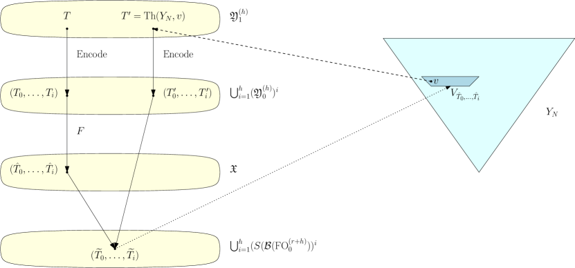
Figure 4.5. Comparing $T$ with its approximation in $Y_{N}$

First note that it is sufficient to prove $T_{i}\cap{\rm FO}_{0}^{(r+h)}=T_{i}^{\prime}\cap{\rm FO}_{0}^{(r+h)}$, as the other equalities follow by considering the ancestors of $v$. If $T_{i}$ (hence $T_{i}^{\prime}$) is the complete theory of a single vertex tree, then by construction of $V_{\hat{T}_{0},\dots,\hat{T}_{i}}$, it holds that $T_{i}=T_{i}^{\prime}$. Assume now that $i$ is such that for every $(T_{0},\dots,T_{i+1})\in{\rm Encode}(T)$ with $T\in\mathfrak{Z}$, it holds that $T_{i+1}\cap{\rm FO}_{0}^{(r+h)}=T_{i+1}^{\prime}\cap{\rm FO}_{0}^{(r+h)}$. Let $A$ be a model of $T_{i}$ and let $B$ be a model of $T_{i}^{\prime}$. It follows from the induction that the roots of $A$ and $B$ have the same number of sons (up to $r+h$) with subtrees, which are $(r+h)$-equivalent to a fixed rooted tree. By an easy argument based on an Ehrenfeucht-Fraïssé game, it follows that $A$ and $B$ are $(r+h)$-equivalent hence $T_{i}\cap{\rm FO}_{0}^{(r+h)}=T_{i}^{\prime}\cap{\rm FO}_{0}^{(r+h)}$.

According to Lemma 4.4, we deduce that for $T\in\mathfrak{Z}$ and the corresponding vertex $v\in V_{\hat{T}_{0},\dots,\hat{T}_{i}}$ it holds that ${\rm Th}(Y_{N},v)\cap{\rm FO}_{1}^{(r)}=T\cap{\rm FO}_{1}^{(r)}$.

It follows that for every $\varphi\in{\rm FO}_{1}^{(r)}$ the following equation holds:

$$\langle\varphi,Y_{N}\rangle=\sum_{(\hat{T}_{0},\dots,\hat{T}_{i})\in\mathcal{F}_{\varphi}}\frac{|V_{\hat{T}_{0},\dots,\hat{T}_{i}}|}{|Y_{N}|}.$$

Hence

$$\bigl{|}\langle\varphi,Y_{N}\rangle-\mu(K(\varphi))\bigr{|}\leq C/N.$$

Let $r_{N}$ be the root of $Y_{N}$. Define

$$\alpha_{N}=\max_{v\sim r_{N}}\frac{|Y_{N}(v)|}{|Y_{N}|}.$$

Assume $\mathbf{L}$ is a modeling with ${\rm FO}_{1}$ statistics $\mu$ and root $r_{\mathbf{L}}$.

Let $(\hat{T}_{0},\hat{T}_{1})\in\mathfrak{X}$ (vertices in $V_{\hat{T}_{0},\hat{T}_{1}}$ are sons of the root of $Y_{N}$). By construction, all the subtrees rooted at a vertex in $V_{\hat{T}_{0},\hat{T}_{1}}$ have almost the same number of vertices (the difference being at most $C$). If $w^{\prime}(\hat{T}_{0},\hat{T}_{1})=r+h$, it follows that for every $v\in V_{\hat{T}_{0},\hat{T}_{1}}$ it holds that $|Y_{N}(v)|\leq C+|Y_{N}|/(r+h)$, i.e. $|Y_{N}(v)|/|Y_{N}|\leq 1/(r+h)+C/N$. Otherwise, $w^{\prime}(\hat{T}_{0},\hat{T}_{1})=k<r+h$ hence if $\psi$ is the formula stating that the ancestor of $x_{1}$ which is a son of the root satisfies $\bigwedge\hat{T}_{1}$, then

$$\mu(K(\psi))=\langle\psi,\mathbf{L}\rangle=\sum_{v\sim r_{\mathbf{L}},\mathbf{L}\models\psi(v)}\nu_{\mathbf{L}}(\mathbf{L}(v))\leq k\sup_{v\sim r_{\mathbf{L}}}\nu_{\mathbf{L}}(\mathbf{L}(v)).$$

Also

$$\mu(K(\psi))+\frac{C}{N}\geq\langle\psi,Y_{N}\rangle =\sum_{(\hat{T}_{0},\dots,\hat{T}_{i})\in\mathcal{F}_{\psi}}\frac{|V_{\hat{T}_{0},\dots,\hat{T}_{i}}|}{|Y_{N}|}$$

$$=\sum_{v\sim r_{N},Y_{n}\models\psi(v)}\frac{|Y_{N}(v)|}{|Y_{N}|}$$

hence $$\mu(K(\psi))+\frac{C}{N}\geq\max_{v\sim r_{N},Y_{n}\models\psi(v)}\frac{|Y_{N}(v)|}{|Y_{N}|} k=1$$ if , and otherwise

$$\mu(K(\psi))+\frac{C}{N} \geq k\max_{v\sim r_{N},Y_{n}\models\psi(v)}\frac{|Y_{N}(v)|-C}{|Y_{N}|}$$

$$\geq k\max_{v\sim r_{N},Y_{n}\models\psi(v)}\frac{|Y_{N}(v)|}{|Y_{N}|}-C/N.$$

Hence, considering the case $$k=1 k\geq 2 2C/k\leq C$$ and the case (where ) we get

$$\max_{v\sim r_{N},Y_{n}\models\psi(v)}\frac{|Y_{N}(v)|}{|Y_{N}|} \leq\sup_{v\sim r_{\mathbf{L}}}\nu_{\mathbf{L}}(\mathbf{L}(v))+C/N.$$

And we deduce

$$\alpha_{N}\leq\max\Bigl{(}\frac{1}{r+h},\sup_{v\sim r_{\mathbf{L}}}\nu_{\mathbf{L}}(\mathbf{L}(v))\Bigr{)}+C/N.$$

∎

Summarizing, we get the following two inverse results:

Theorem 4.23.

A measure $\mu$ on $S(\mathcal{B}({\rm FO}_{1}))$ is the weak limit of a sequence of measures $\mu_{Y_{n}}$ associated to an ${\rm FO}_{1}$-convergent sequence $(Y_{n})_{n\in\mathbb{N}}$ of finite colored rooted trees with height at most $h$ (i.e. of finite $Y_{n}\in\mathcal{Y}^{(h)}$) if and only if

• $\mu$ is pure and its complete theory belongs to $\mathfrak{Y}_{0}^{(h)}$,

• $\mu$ satisfies the FMTP.

Proof.

Assume that $(Y_{n})_{n\in\mathbb{N}}$ is an ${\rm FO}_{1}$-convergent sequence of finite $Y_{n}\in\mathcal{Y}^{(h)}$, and that $\mu_{Y_{N}}\Rightarrow\mu$. According to Remark 2.10, $\mu$ is pure. As $(Y_{n})_{n\in\mathbb{N}}$ is elementarily convergent, the complete theory of $\mu$ is the complete theory of the elementary limit of $(Y_{n})_{n\in\mathbb{N}}$. Also, $\mu$ satisfies the FMTP (see Section 2.1.4).

Conversely, assume $\mu$ is pure, that its complete theory belongs to $\mathfrak{Y}_{0}^{(h)}$, and that it satisfies the FMTP. According to Lemma 4.22 we can construct a sequence $(Y_{n})_{n\in\mathbb{N}}$ of finite $Y_{n}\in\mathcal{Y}^{(h)}$ (considering for instance $r=n$ and $N=10^{C}$ where $C$ is the constant defined from $r,h,c$) such that for every formula $\phi\in{\rm FO}_{1}(\lambda)$ it holds that $\bigl{|}\langle\phi,Y_{n}\rangle-\mu(K(\phi))\bigr{|}\rightarrow 0$ as $n\rightarrow\infty$, i.e. $\mu_{Y_{n}}\Rightarrow\mu$. ∎

From this we deduce

Theorem 4.24.

A modeling $\mathbf{L}$ is the ${\rm FO}_{1}$-limit of an ${\rm FO}_{1}$-convergent sequence $(Y_{n})_{n\in\mathbb{N}}$ of finite colored rooted trees with height at most $h$ (i.e. of finite $Y_{n}\in\mathcal{Y}^{(h)}$) if and only if

• $\mathbf{L}$ is a colored rooted tree with height at most $h$ (i.e. $\mathbf{L}\in\mathcal{Y}^{(h)}$),

• ${\mathbf{L}}$ satisfies the FMTP.

Proof.

That an ${\rm FO}_{1}$-convergent sequence of finite rooted colored trees $Y_{n}\in\mathcal{Y}^{(h)}$ has a modeling ${\rm FO}_{1}$-limit is a direct consequence of Theorem 4.18. That ${\mathbf{L}}$ satisfies the FMTP is immediate (as the associated measure $\mu=\tensor*[^{1}_{\scriptscriptstyle\mathbf{L}}]{\sf\textstyle Tp}{}_{*}(\nu_{\mathbf{L}})$ does).

Conversely, that a colored rooted tree modeling $\mathbf{L}\in\mathcal{Y}^{(h)}$ that satisfies the FMTP is the ${\rm FO}_{1}$-limit of a sequence of finite rooted colored trees $Y_{n}\in\mathcal{Y}^{(h)}$ is a direct consequence of Theorem 4.23. ∎

4.2. ${\rm FO}$-limits of Colored Rooted Trees with Bounded Height

In this section we explicitly define modeling ${\rm FO}$-limits for ${\rm FO}$-convergent sequences of colored rooted trees with bounded height.

We first sketch our method.

We consider the signature $\lambda^{+}$, which is the signature $\lambda$ augmented by a new unary relation $P$. Particular $\lambda^{+}$-structures are colored rooted forests with a principal connected component, whose root will be marked by relation $P$ instead of $R$ (no other vertex gets $P$). The class of colored rooted forests with a principal connected component and height at most $h$ will be denoted by $\mathcal{F}^{(h)}$.

We consider three basic interpretation schemes:

1. $\mathsf{I}_{Y\rightarrow F}$ is a basic interpretation scheme of $\lambda^{+}$-structures in $\lambda$-structures defined as follows: for every $\lambda$-structure $\mathbf{A}$, the domain of $\mathsf{I}_{Y\rightarrow F}(\mathbf{A})$ is the same as the domain of $\mathbf{A}$, and the following holds (for every $x,y\in A$):

   $$\mathsf{I}_{Y\rightarrow F}(\mathbf{A})\models x\sim y \quad\iff\quad\mathbf{A}\models(x\sim y)\wedge\neg R(x)\wedge\neg R(y)$$

   $$\mathsf{I}_{Y\rightarrow F}(\mathbf{A})\models R(x) \quad\iff\quad\mathbf{A}\models(\exists z)\ R(z)\wedge(z\sim x)$$

   $$\mathsf{I}_{Y\rightarrow F}(\mathbf{A})\models P(x) \quad\iff\quad\mathbf{A}\models R(x)$$

   In particular, $\mathsf{I}_{Y\rightarrow F}$ maps a colored rooted tree $Y\in\mathcal{Y}^{(h)}$ into a colored rooted forest $\mathsf{I}_{Y\rightarrow F}(\mathbf{A})(Y)\in\mathcal{F}^{(h-1)}$, formed by the subtrees rooted at the sons of the former root and a single vertex rooted principal component (the former root);

2. $\mathsf{I}_{F\rightarrow Y}$ is a basic interpretation scheme of $\lambda$-structures in $\lambda^{+}$-structures defined as follows: for every $\lambda^{+}$-structure $\mathbf{A}$, the domain of $\mathsf{I}_{F\rightarrow Y}(\mathbf{A})$ is the same as the domain of $\mathbf{A}$, and the following holds (for every $x,y\in A$):

   $$\mathsf{I}_{F\rightarrow A}(\mathbf{A})\models x\sim y \quad\iff\quad\mathbf{A}\models(x\sim y)\vee R(x)\wedge P(y)\vee R(y)\wedge P(x)$$

   $$\mathsf{I}_{F\rightarrow A}(\mathbf{A})\models R(x) \quad\iff\quad\mathbf{A}\models P(x)$$

   In particular, $\mathsf{I}_{F\rightarrow Y}$ maps a colored rooted forest $F\in\mathcal{F}^{(h)}$ into a colored rooted tree $\mathsf{I}_{F\rightarrow Y}(F)\in\mathcal{Y}^{(h+1)}$ by making each non-principal root a son of the principal root;

3. $\mathsf{I}_{R\rightarrow P}$ is a basic interpretation scheme of $\lambda^{+}$-structures in $\lambda$-structures defined as follows: for every $\lambda^{+}$-structure $\mathbf{A}$, the domain of $\mathsf{I}_{R\rightarrow P}(\mathbf{A})$ is the same as the domain of $\mathbf{A}$, adjacencies are the same in $\mathbf{A}$ and $\mathsf{I}_{R\rightarrow P}(\mathbf{A})$, no element of $\mathsf{I}_{R\rightarrow P}(\mathbf{A})$ is in $R$, and for every $x\in A$ the following equivalence holds:

   $$I_{R\rightarrow P}(\mathbf{A})\models P(x)\quad\iff\quad\mathbf{A}\models R(x).$$

   (Roughly speaking, the relation $R$ becomes the relation $P$.) In particular, $\mathsf{I}_{R\rightarrow P}$ maps a colored rooted tree $Y\in\mathcal{Y}^{(h)}$ into a colored rooted forest $\mathsf{I}_{R\rightarrow P}(Y)\in\mathcal{F}^{(h)}$ having a single (principal) component.

We now outline our proof strategy. Let $(\mathbf{Y}_{n})_{n\in\mathbb{N}}$ be an ${\rm FO}$-convergent sequence of finite rooted colored trees ($\mathbf{Y}_{n}\in\mathcal{Y}^{(h)}$) such that $\lim_{n\rightarrow\infty}|Y_{n}|=\infty$.

For each $n$, $\mathsf{I}_{Y\rightarrow F}(\mathbf{Y}_{n})$ is a forest $\mathbf{F}_{n}$, and $(\mathbf{Y}_{n})_{n\in\mathbb{N}}$ is an ${\rm FO}$-convergent sequence. According to the Comb Structure Theorem, there exists a countable set $(\mathbf{Y}_{n,i})_{n\in\mathbb{N}}$ of ${\rm FO}$-convergent sequences of colored rooted trees $\mathbf{Y}_{n,i}\in\mathcal{Y}^{(h)}$ and a ${\rm FO}$-convergent sequence $(\mathbf{R}_{n})_{n\in\mathbb{N}}$ of residues $\mathbf{R}_{n}\in\mathcal{F}^{(h)}$, which are special colored rooted forests (as the isolated principal root obviously belongs to $\mathbf{R}_{n}$), so that

• the sequences $(\mathbf{Y}_{n,i})_{n\in\mathbb{N}}$ and the sequence $(\mathbf{R}_{n})_{n\in\mathbb{N}}$ form a uniformly convergent family of sequences;

• for each $n\in\mathbb{N}$ it holds that $\mathsf{I}_{Y\rightarrow F}(\mathbf{Y}_{n})=\mathbf{R}_{n}\cup\bigcup_{i\in I}\mathbf{Y}_{n,i}$.

If the limit spectrum of $(\mathsf{I}_{Y\rightarrow F}(\mathbf{Y}_{n}))_{n\in\mathbb{N}}$ is empty (i.e. $I=\emptyset$), the sequence $(\mathbf{Y}_{n})_{n\in\mathbb{N}}$ of colored rooted trees is called residual, and in this case we deduce directly that a residual sequence of colored rooted trees admit a modeling ${\rm FO}$-limit from our results on ${\rm FO}_{1}$-convergent sequences.

Otherwise, we proceed by induction over the height bound $h$. Denote by $(\hskip 1.0pt\mathsf{sp}_{i})_{i\in I}$ the limit spectrum of $(\mathsf{I}_{Y\rightarrow F}(\mathbf{Y}_{n}))_{n\in\mathbb{N}}$, let $\hskip 1.0pt\mathsf{sp}_{0}=1-\sum_{i\in I}\hskip 1.0pt\mathsf{sp}_{i}$, and let $\mathbf{Y}_{n,0}=\mathsf{I}_{R\rightarrow P}\circ\mathsf{I}_{F\rightarrow Y}(\mathbf{R}_{n})$. As $(\mathsf{I}_{F\rightarrow Y}(\mathbf{R}_{n}))_{n\in\mathbb{N}}$ is residual, $(\mathbf{Y}_{n,0})_{n\in\mathbb{N}}$ has a modeling FO-limit $\widetilde{\mathbf{Y}}_{0}$. By induction, each $(\mathbf{Y}_{n,i})_{n\in\mathbb{N}}$ has a modeling FO-limit $\widetilde{\mathbf{Y}}_{i}$. As $\mathbf{Y}_{n}=\mathsf{I}_{F\rightarrow Y}(\bigcup_{i\in I\cup\{0\}}{\mathbf{Y}}_{n,i})$, we deduce (using uniform elementary convergence) that $(\mathbf{Y}_{n})_{n\in\mathbb{N}}$ has modeling ${\rm FO}$-limit $\mathsf{I}_{F\rightarrow Y}(\coprod_{i\in I\cup\{0\}}(\widetilde{\mathbf{Y}}_{i},\hskip 1.0pt\mathsf{sp}_{i}))$.

This finishes the outline of our construction. Now we provide details.

4.2.1. The Modeling FO-limit of Residual Sequences

We start by a formal definition of residual sequences of colored rooted trees.

Definition 4.25.

Let $(\mathbf{Y}_{n})_{n\in\mathbb{N}}$ be a sequence of finite colored rooted trees, let $N_{n}$ be the set of all sons of the root of $\mathbf{Y}_{n}$, and let $\mathbf{Y}_{n}(v)$ denote (for $v\in Y_{n}$) the subtree of $\mathbf{Y}_{n}$ rooted at $v$.

The sequence $(\mathbf{Y}_{n})_{n\in\mathbb{N}}$ is residual if

$$\limsup_{n\rightarrow\infty}\max_{v\in N_{n}}\frac{|\mathbf{Y}_{n}(v)|}{|\mathbf{Y}_{n}|}=0.$$

We extend this definition to single infinite modelings.

Definition 4.26.

A modeling colored rooted tree $\widetilde{\mathbf{Y}}$ with height at most $h$ is residual if, denoting by $N$ the neighbor set of the root, it holds that

$$\sup_{v\in N}\nu_{\widetilde{\mathbf{Y}}}(\widetilde{\mathbf{Y}}(v))=0.$$

Note that the above definition makes sense as belonging to some $\widetilde{\mathbf{Y}}(v)$ (for some $v\in N$) is first-order definable hence, as $\widetilde{\mathbf{Y}}$ is a relational sample space, each $\widetilde{\mathbf{Y}}(v)$ is $\Sigma_{\widetilde{\mathbf{Y}}}$-measurable.

We first prove that for a modeling colored rooted tree to be a modeling ${\rm FO}$-limit of a residual sequence $(\mathbf{Y}_{n})_{n\in\mathbb{N}}$ of rooted colored trees with bounded height, it is sufficient that it is a modeling ${\rm FO}_{1}$-limit of the sequence.

Lemma 4.27.

Assume $(\mathbf{Y}_{n})_{n\in\mathbb{N}}$ is a residual ${\rm FO}_{1}$-convergent sequence of finite rooted colored trees with bounded height with residual modeling ${\rm FO}_{1}$-limit $\widetilde{\mathbf{Y}}$.

Then $(\mathbf{Y}_{n})_{n\in\mathbb{N}}$ is ${\rm FO}$-convergent and has modeling ${\rm FO}$-limit $\widetilde{\mathbf{Y}}$.

Proof.

Let $h$ be a bound on the height of the rooted trees $\mathbf{Y}_{n}$. Let $\mathbf{F}_{n}=I_{Y\rightarrow F}(\mathbf{Y}_{n})$. Let $\varpi$ be the formula asserting ${\rm dist}(x_{1},x_{2})\leq 2h$. Then $\mathbf{F}_{n}\models\varpi(u,v)$ holds if and only if $u$ and $v$ belong to a same connected component of $\mathbf{F}_{n}$. According to Lemma 3.54, we get that $(\mathbf{F}_{n})_{n\in\mathbb{N}}$ is ${\rm FO}^{\rm local}$-convergent. As it is also ${\rm FO}_{0}$-convergent, it is ${\rm FO}$-convergent (according to Theorem 2.23). As $\mathbf{Y}_{n}=I_{F\rightarrow Y}(\mathbf{F}_{n})$, we deduce that $(\mathbf{Y}_{n})_{n\in\mathbb{N}}$ is ${\rm FO}$-convergent.

That $\widetilde{\mathbf{Y}}$ is a modeling FO-limit of $(\mathbf{Y}_{n})_{n\in\mathbb{N}}$ then follows from Theorem 3.22. ∎

Lemma 4.28.

Let $\mathbf{Y}_{n}$ be a residual ${\rm FO}_{1}$-convergent sequence of colored rooted trees with height at most $h$, let $\mu$ be the limit measure of $\mu_{\mathbf{Y}_{n}}$ on $\mathfrak{T}_{1}^{(h)}$, and let $\widetilde{\mathbf{Y}}$ be the connected component of $\mathbb{Y}_{h}$ containing the support of $\nu$. Then $\widetilde{\mathbf{Y}}$, equipped with the probability measure $\nu_{\widetilde{\mathbf{Y}}}=\nu$, is a modeling ${\rm FO}$-limit of $(\mathbf{Y}_{n})_{n\in\mathbb{N}}$.

Proof.

That $\widetilde{\mathbf{Y}}$ is a residual ${\rm FO}_{1}$-modeling limit of $(\mathbf{Y}_{n})_{n\in\mathbb{N}}$ is a consequence of Theorem 4.18. That it is then an ${\rm FO}$-modeling limit of $(\mathbf{Y}_{n})_{n\in\mathbb{N}}$ follows from Lemma 4.27 ∎

4.2.2. The Modeling ${\rm FO}$-Limit of a Sequence of Rooted Trees

For an intuition of how the structure of a modeling FO-limit of a sequence of colored rooted trees with height at most $h$ could look like, consider a modeling rooted colored tree $\mathbf{Y}$. Obviously, the $\mathbf{Y}$ contains two kind of vertices: the heavy vertices $v$ such that the subtree $\mathbf{Y}(v)$ of $\mathbf{Y}$ rooted at $v$ has positive $\nu_{\mathbf{Y}}$-measure and the light vertices for which $\mathbf{Y}(v)$ has zero $\nu_{\mathbf{Y}}$-measure. It is then immediate that heavy vertices of $\mathbf{Y}$ induce a countable rooted subtree with same root as $\mathbf{Y}$.

This suggest the following definitions.

Definition 4.29.

A rooted skeleton is a countable rooted tree $\mathbf{S}$ together with a mass function $m:S\rightarrow(0,1]$ such that $m(r)=1$ ($r$ is the root of $\mathbf{S}$) and for every non-leaf vertex $v\in S$ it holds that

$$m(v)\geq\sum_{u\text{ son of }v}m(u).$$

Definition 4.30.

Let $(\mathbf{S},m)$ be a rooted skeleton, let $S_{0}$ be the subset of $S$ with vertices $v$ such that $m(v)=\sum_{u\text{ son of }v}m(u)$, let $(\mathbf{R}_{v})_{v\in S\setminus S_{0}}$ be a countable sequence of non-empty residual $\lambda$-modeling indexed by $S\setminus S_{0}$, and let $(\mathbf{R}_{v})_{v\in S_{0}}$ be a countable sequence of non empty countable colored rooted trees indexed by $S_{0}$. The grafting of $(\mathbf{R}_{v})_{v\in S\setminus S_{0}}$ and $(\mathbf{R}_{v})_{v\in S_{0}}$ on $(\mathbf{S},m)$ is the modeling $\mathbf{Y}$ defined as follows: As a graph, $\mathbf{Y}$ is obtained by taking the disjoint union of $\mathbf{S}$ with the colored rooted trees $\mathbf{R}_{v}$ and then identifying $v\in S$ with the root of $\mathbf{R}_{v}$ (see Fig. 4.6). The sigma algebra $\Sigma_{\mathbf{Y}}$ is defined as

$$\Sigma_{\mathbf{Y}}=\Bigl{\{}\bigcup_{v\in S\setminus S_{0}}M_{v}\cup\bigcup_{v\in S_{0}}M_{v}^{\prime}:\ M_{v}\in\Sigma_{\mathbf{R}_{v}},M_{v}^{\prime}\subseteq R_{v}\Bigr{\}}$$

and the measure $\nu_{\mathbf{Y}}(M)$ of $M\in\Sigma$ is defined by

$$\nu_{\mathbf{Y}}(M)=\sum_{v\in S\setminus S_{0}}\Bigl{(}m(v)-\sum_{u\text{ son of }v}m(u)\Bigr{)}\nu_{\mathbf{R}_{v}}(M_{v}),$$

where $M=\bigcup_{v\in S\setminus S_{0}}M_{v}\cup\bigcup_{v\in S}M_{v}^{\prime}$ with $M_{v}\in\Sigma_{\mathbf{R}_{v}}$ and $M_{v}^{\prime}\subseteq R_{v}$.

Figure 4.6. Grafting of trees on a skeleton

Lemma 4.31.

Let $\mathbf{Y}$ be obtained by grafting a countable sequence of non-empty modeling colored rooted trees $\mathbf{R}_{v}$ on a rooted skeleton $(\mathbf{S},m)$. Then $\mathbf{Y}$ is a modeling.

Proof.

We prove the statement by induction over the height of the rooted skeleton. The statement obviously holds if $\mathbf{S}$ is a single vertex rooted tree (that is if ${\rm height}(\mathbf{S})=1$). Assume that the statement holds for rooted skeletons with height at most $h$, and let $(\mathbf{S},m)$ be a rooted skeleton with height $h+1$.

Let $s_{0}$ be the root of $\mathbf{S}$ and let $\{s_{i}:i\in I\subseteq\mathbb{N}\}$ be the set of the sons of $s_{0}$ in $\mathbf{S}$. For $i\in I$, $\mathbf{Y}_{i}=\mathbf{Y}(s_{i})$ be the subtree of $\mathbf{Y}$ rooted at $s_{i}$, let $\hskip 1.0pt\mathsf{sp}_{i}=\sum_{x\in Y_{i}}m(x)$, and let $m_{i}$ be the mass function on $\mathbf{S}_{i}$ defined by $m_{i}(v)=m(v)/\hskip 1.0pt\mathsf{sp}_{i}$. Also, let $\hskip 1.0pt\mathsf{sp}_{0}=1-\sum_{i\in I}\hskip 1.0pt\mathsf{sp}_{i}$.

For each $i\in I\cup\{0\}$, if $\hskip 1.0pt\mathsf{sp}_{i}=0$ (in which case $\mathbf{R}_{s_{i}}$ is only assumed to be a relational sample space) we turn $\mathbf{R}_{s_{i}}$ into a modeling by defining a probability measure on $\mathbf{R}_{s_{i}}$ concentrated on $s_{i}$.

For $i\in I$, let $\mathbf{Y}_{i}$ be obtained by grafting the $\mathbf{R}_{v}$ on $(\mathbf{S}_{i},m_{i})$ (for $v\in S_{i}$), and let $\mathbf{Y}_{0}$ be the $\lambda^{+}$-modeling consisting in a rooted colored forest with single (principal) component $\mathbf{R}_{s_{0}}$ (that is: $\mathbf{Y}_{0}=\mathsf{I}_{R\rightarrow P}(\mathbf{R}_{s_{0}}))$. According to Lemma 3.13, $\mathbf{Y}_{0}$ is a modeling, and by induction hypothesis each $\mathbf{Y}_{i}$ ($i\in I$) is a modeling. According to Lemma 3.26, it follows that $\mathbf{F}=\amalg_{i\in I\cup\{0\}}(\mathbf{Y}_{i},\hskip 1.0pt\mathsf{sp}_{i})$ is a modeling. Hence, according to Lemma 3.13, $\mathbf{Y}=\mathsf{I}_{F\rightarrow Y}(\mathbf{F})$ is a modeling. ∎

Our main theorem is the following.

Theorem 4.32.

Let $(\mathbf{Y}_{n})_{n\in\mathbb{N}}$ be an ${\rm FO}$-convergent sequence of finite colored rooted trees with height at most $h$.

Then there exists a skeleton $(\mathbf{S},m)$ and a family $(\mathbf{R}_{v})_{v\in S}$ — where $\mathbf{R}_{v}$ is (isomorphic to) a connected component of $\mathbb{Y}_{h}$, $\Sigma_{\mathbf{R}_{v}}$ is the induced $\sigma$-algebra on $R_{v}$ — with the property that the grafting $\mathbf{Y}$ of the $\mathbf{R}_{v}$ on $(\mathbf{S},m)$ is a modeling ${\rm FO}$-limit of the sequence $(\mathbf{Y}_{n})_{n\in\mathbb{N}}$.

Proof.

First notice that the statement obviously holds if $\lim_{n\rightarrow\infty}|Y_{n}|<\infty$ as then the sequence is eventually constant to a finite colored rooted tree $\mathbf{Y}$: we can let $\mathbf{S}$ be $\mathbf{Y}$ (without the colors), $m$ be the uniform weight ($m(v)=1/|Y|$), and $\mathbf{R}_{v}$ be single vertex rooted tree whose root’s color is the color of $v$ in $\mathbf{Y}$. So, we can assume that $\lim_{n\rightarrow\infty}|Y_{n}|=\infty$.

We prove the statement by induction over the height bound $h$. For $h=1$, each $\mathbf{Y}_{n}$ is a single vertex colored rooted tree, and the statement obviously holds.

Assume that the statements holds for $h=h_{0}-1\geq 1$ and let finite colored rooted trees with height at most $h_{0}$. Let $\mathbf{F}_{n}=\mathsf{I}_{Y\rightarrow F}(\mathbf{Y}_{n})$. Then $(\mathbf{F}_{n})_{n\in\mathbb{N}}$ is FO-convergent (according to Lemma 3.13). According to the Comb Structure Theorem, there exists countably many convergent sequences $(\mathbf{Y}_{n,i})_{n\in\mathbb{N}}$ of colored rooted trees (for $i\in I$) and an ${\rm FO}$-convergent sequence $(\mathbf{R}_{n})_{n\in\mathbb{N}}$ of special rooted forests forming a uniformly convergent family of sequences, such that $\mathsf{I}_{Y\rightarrow F}(\mathbf{Y}_{n})=\mathbf{R}_{n}\cup\bigcup_{i\in I}\mathbf{Y}_{n,i}$.

If the limit spectrum of $(\mathsf{I}_{Y\rightarrow F}(\mathbf{Y}_{n}))_{n\in\mathbb{N}}$ is empty (i.e. $I=\emptyset$), the sequence $(\mathbf{Y}_{n})_{n\in\mathbb{N}}$ of colored rooted trees is residual, and the result follows from Lemma 4.28.

Otherwise, let $(\hskip 1.0pt\mathsf{sp}_{i})_{i\in I}$ the limit spectrum of $(\mathsf{I}_{Y\rightarrow F}(\mathbf{Y}_{n}))_{n\in\mathbb{N}}$, let $\hskip 1.0pt\mathsf{sp}_{0}=1-\sum_{i\in I}\hskip 1.0pt\mathsf{sp}_{i}$, and let $\mathbf{Y}_{n,0}=\mathsf{I}_{R\rightarrow P}\circ\mathsf{I}_{F\rightarrow Y}(\mathbf{R}_{n})$. If $\hskip 1.0pt\mathsf{sp}=0$ then there is a connected component $\widetilde{\mathbf{Y}}_{0}$ of $\mathbb{Y}_{h}$ that is an elementary limit of $(\mathbf{Y}_{n,0})_{n\in\mathbb{N}}$; otherwise, as $(\mathsf{I}_{F\rightarrow Y}(\mathbf{R}_{n}))_{n\in\mathbb{N}}$ is residual, $(\mathbf{Y}_{n,0})_{n\in\mathbb{N}}$ has, according to Lemma 4.28, a modeling FO-limit $\widetilde{\mathbf{Y}}_{0}$. By induction, each $(\mathbf{Y}_{n,i})_{n\in\mathbb{N}}$ has a modeling FO-limit $\widetilde{\mathbf{Y}}_{i}$. As $\mathbf{Y}_{n}=\mathsf{I}_{F\rightarrow Y}(\bigcup_{i\in I\cup\{0\}}{\mathbf{Y}}_{n,i})$, we deduce, by Corollary 3.31, Lemma 3.33, Theorem 2.23, and Lemma 3.13, that $(\mathbf{Y}_{n})_{n\in\mathbb{N}}$ has modeling ${\rm FO}$-limit $\mathsf{I}_{F\rightarrow Y}(\coprod_{i\in I\cup\{0\}}(\widetilde{\mathbf{Y}}_{i},\hskip 1.0pt\mathsf{sp}_{i}))$. ∎

So, in the case of colored rooted trees with bounded height, we have constructed an explicit relational sample space that allows one to pullback the limit measure $\mu$ defined on the Stone space $S({\mathcal{B}}({\rm FO}))$.

4.2.3. Inverse theorem for ${\rm FO}$-limits of Colored Rooted Trees with Bounded Height

Recall that for $\lambda$-modelings $\mathbf{A}$ and $\mathbf{B}$, and $p,r\in\mathbb{N}$ we defined

$$\|\mathbf{A}-\mathbf{B}\|_{p,r}^{\rm local}=\sup\{|\langle\phi,\mathbf{A}\rangle-\langle\phi,\mathbf{B}\rangle|:\ \phi\in{\rm FO}_{p}^{\rm local}(\lambda),{\rm qrank}(\phi)\leq r\}.$$

Lemma 4.33.

Let $\mathbf{L}\in\mathcal{Y}^{(h)}$ (with root $r_{\mathbf{L}}$) be a colored rooted tree modeling that satisfies the FMTP, let $p,r\in\mathbb{N}$, and let $\epsilon>0$. Then there exist $C_{0}=C_{0}(\lambda,p,r,\epsilon),N_{0}=N_{0}(\lambda,p,r,\epsilon)$ such that for every $N\geq N_{0}$ there exists a finite colored rooted tree $Y\in\mathcal{Y}^{(h)}$ such that it holds that $N\leq|Y|\leq N+C_{0}$, $Y\equiv^{r}\mathbf{L}$, and

$$\|Y-\mathbf{L}\|_{p,r}^{\rm local}<\max(\epsilon,2\sup_{v\sim r_{\mathbf{L}}}\nu_{\mathbf{L}}(\mathbf{L}(v))).$$

Proof.

Without loss of generality we can assume $\epsilon\geq 2\sup_{v\sim r_{\mathbf{L}}}\nu_{\mathbf{L}}(\mathbf{L}(v))$. Let $r^{\prime}=\max(r,4c_{r,p}/\epsilon)$, where $c_{r,p}$ is the constant introduced in Lemma 3.28..

According to Lemma 4.22, there is $C_{0}=C(\lambda,r^{\prime})$ (hence $C_{0}$ depends on $\lambda,p,r$, and $\epsilon$) such that for every $N\in\mathbb{N}$ there exists $Y\in\mathcal{Y}^{(h)}$ with the following properties:

1. $N\leq|Y|\leq N+C_{0}$;

2. for every $\varphi\in{\rm FO}_{1}$ with quantifier rank at most $r^{\prime}$ the following inequality holds

   $$\bigl{|}\langle\varphi,Y\rangle-\langle\varphi,\mathbf{L}\rangle\bigr{|}\leq C_{0}/N.$$

   (In particular $Y\equiv^{r^{\prime}}\mathbf{L}$ as $N>C_{0}$.)

3. we have

   $$\max_{v\sim r_{N}}\frac{|Y(v)|}{|Y|}\leq\max\Bigl{(}\frac{1}{r^{\prime}+h},\sup_{v\sim r_{\mathbf{L}}}\nu_{\mathbf{L}}(\mathbf{L}(v))\Bigr{)}+C_{0}/N.$$

Let $N_{0}=4c_{r,p}C(\lambda,r^{\prime})/\epsilon$ and assume $N\geq N_{0}$.

Let $F={\mathsf{I}}_{Y\rightarrow F}(Y)$ and $\mathbf{A}={\mathsf{I}}_{Y\rightarrow F}(\mathbf{L})$. Let $F_{i},i\in\Gamma_{F}$ and $\mathbf{A}_{i},i\in\Gamma_{\mathbf{A}}$ be the connected components of $F$ and $\mathbf{A}$. Then

$$\max_{i\in\Gamma_{F}}\frac{|F_{i}|}{|F|}\leq\max\Bigl{(}\frac{1}{r^{\prime}+h},\sup_{i\in\Gamma_{\mathbf{L}}}\nu_{\mathbf{A}}(\mathbf{A}_{i})\Bigr{)}+C_{0}/N<\frac{\epsilon}{2c_{r,p}}.$$

As ${\mathsf{I}}_{Y\rightarrow F}$ is a quantifier free interpretation, for every $\varphi\in{\rm FO}_{1}$ with quantifier rank at most $r$ the following inequality holds

$$\bigl{|}\langle\varphi,F\rangle-\langle\varphi,\mathbf{A}\rangle\bigr{|}\leq C_{0}/N\leq\frac{\epsilon}{4c_{r,p}}.$$

In particular we have $\|F-\mathbf{A}\|_{1,r}^{\rm local}\leq\frac{\epsilon}{4c_{r,p}}$. According to Lemma 3.29, it holds that

$$\|F-\mathbf{A}\|_{p,r}^{\rm local} <c_{r,p}\biggl{(}\max_{i\in\Gamma_{F}}\frac{|F_{i}|}{|F|}+\sup_{i\in\Gamma_{\mathbf{L}}}\nu_{\mathbf{A}}(\mathbf{A}_{i})+\|F-\mathbf{A}\|_{1,r}^{\rm local}\biggr{)}<\epsilon.$$

and it follows that $\|Y-\mathbf{L}\|_{p,r}^{\rm local}<\epsilon$. ∎

Lemma 4.34.

Let $\mathbf{L}\in\mathcal{Y}^{(h)}$ be an infinite colored rooted tree modeling that satisfies the FMTP, let $p,r\in\mathbb{N}$ and let $\epsilon>0$. Then there exist constants $C_{h},N_{h}$ (depending on $\lambda,p,r,\epsilon$) such that for every $N\geq N_{h}$ there is a finite colored rooted tree $Y_{\epsilon}\in\mathcal{Y}^{(h)}$ such that $N\leq|Y_{\epsilon}|\leq N+C_{h}$, $Y_{\epsilon}\equiv^{r}\mathbf{L}$, and $\|\mathbf{L}-Y_{\epsilon}\|_{p,r}^{\rm local}<\epsilon$.

Proof.

Let $\alpha=\epsilon^{2}/(2(3c_{r,p})^{h})$, where $c_{r,p}$ is the constant which appears in Lemma 3.28. A vertex $v\in L$ is $\alpha$-heavy if either $v$ is the root $r_{\mathbf{L}}$ of $\mathbf{L}$, or the father $u$ of $v$ in $\mathbf{L}$ is $\alpha$-heavy and $\nu_{\mathbf{L}}(\mathbf{L}(v))>\alpha\nu_{\mathbf{L}}(\mathbf{L}(u))$. The $\alpha$-heavy vertices of $\mathbf{L}$ form a finite subtree $S$ rooted at $r_{\mathbf{L}}$ (each node $v$ of $S$ has at most $1/\alpha$ sons).

We prove by induction on the height $t$ of $S$ that — assuming $\alpha\leq\epsilon/2$ — there exist constants $C_{t-1},N_{t-1}$ (depending on $\lambda,p,r,\epsilon$) such that for every $N\geq N_{t-1}$ there is a finite colored rooted tree $Y_{\epsilon}\in\mathcal{Y}^{(h)}$ such that $N\leq|Y_{\epsilon}|\leq N+C_{t-1}$, $Y_{\epsilon}\equiv^{r}\mathbf{L}$, and $\|\mathbf{L}-Y_{\epsilon}\|_{p,r}^{\rm local}<\epsilon$.

If $t=1$ (i.e. $r_{\mathbf{L}}$ is the only $\alpha$-heavy vertex) then

$$\sup_{v\sim r_{\mathbf{L}}}\nu_{\mathbf{L}}(\mathbf{L}(v))<\alpha.$$

Hence, according to Lemma 4.33, there exists $N_{0},C_{0}$ (depending on $\lambda,r,p$, and $\epsilon$) such that for every $N\geq N_{0}$ there is a finite colored rooted tree $Y\in\mathcal{Y}^{(h)}$ such that $N\leq|Y|\leq N+C_{0}$, $Y\equiv^{r}\mathbf{L}$, and

$$\|Y-\mathbf{L}\|_{p,r}^{\rm local}<\max(\epsilon,2\sup_{v\sim r_{\mathbf{L}}}\nu_{\mathbf{L}}(\mathbf{L}(v)))=\epsilon.$$

Now assume that the statement we want to prove by induction holds when $S$ has height at most $t\geq 1$, and let $\mathbf{L}$ be such that the associated subtree $S$ of $\alpha$-heavy vertices has height $t+1$. Let $v_{1},\dots,v_{k}$ (where $k$ is at most $1/\alpha$) be the $\alpha$-heavy sons of the root $r_{\mathbf{L}}$ of $\mathbf{L}$, let $\mathbf{L}_{i}$ be the relational sample space defined by $\mathbf{L}_{i}=\mathbf{L}(v_{i})$ for $1\leq i\leq k$, and let $\mathbf{L}_{0}$ be the colored rooted tree relational sample space obtained by removing all the subtrees $\mathbf{L}_{i}$ from $\mathbf{L}$. Each $L_{i}$ is measurable in $\mathbf{L}$. Let $a_{i}=\nu_{\mathbf{L}}(\mathbf{L}_{i})$, and let

$$\epsilon^{\prime} =\frac{\epsilon}{3c_{r,p}}$$

$$C_{t}(\lambda,p,r,\epsilon) =\max\biggl{(}\frac{C_{t-1}(\lambda,p,r,\epsilon^{\prime})}{\alpha},C_{0}(\lambda,p,r,\epsilon^{\prime}/3c_{r,p})\biggr{)}$$

$$N_{t}(\lambda,p,r,\epsilon) =\max\biggl{(}\frac{N_{t-1}(\lambda,p,r,\epsilon^{\prime})}{\epsilon^{\prime}},\frac{C_{t-1}(\lambda,p,r,\epsilon^{\prime})}{\alpha\epsilon^{\prime}},N_{0}(\lambda,p,r,\epsilon^{\prime}/3c_{r,p})\biggr{)}.$$

(Note that we do not change $\alpha$.)

Assume $a_{0}\geq\epsilon^{\prime}$. Let $\mathbf{\hat{L}_{i}}$ be the modeling with relational sample space ${\mathbf{L}_{i}}$ and probability measure $\nu_{\mathbf{\hat{L}_{i}}}$ which is $a_{i}^{-1}\nu_{\mathbf{L}}|L_{i}$, where $\nu_{\mathbf{L}}|L_{i}$ stands for the restriction of $\nu_{\mathbf{L}}$ to $L_{i}$. Let $S_{i}$ be the rooted subtree of $\alpha$-heavy vertices of $\mathbf{\hat{L}_{i}}$. Clearly, if $1\leq i\leq k$, then $S_{i}=S(v_{i})$ (as we did not change $\alpha$) thus $S_{i}$ has height at most $t$. Let $\mathbf{F}\in\mathcal{F}^{(h)}$ be the forest defined from $\mathbf{F}=\coprod_{i=0}^{k}(\mathbf{\hat{L}_{i}},a_{i})$ by making the component $\mathbf{\hat{L}_{0}}$ special. It is clear that $\mathbf{L}={\mathsf{I}}_{F\rightarrow Y}(\mathbf{F})$. For every $N\geq N_{t}(\lambda,p,r,\epsilon)\geq N_{t-1}(\lambda,p,r,\epsilon^{\prime})/\epsilon^{\prime}$ there exist, by induction, $Y_{1},\dots,Y_{k}$ such that $a_{i}N\leq Y_{i}\leq a_{i}N+C_{t-1}(\lambda,p,r,\epsilon^{\prime})$, $Y_{i}\equiv^{r}\mathbf{\hat{L}_{i}}$, and $\|Y_{i}-\mathbf{\hat{L}_{i}}\|_{p,r}^{\rm local}<\epsilon^{\prime}$. As the induction step is carried on at most $h$ times, it will always hold that $\alpha\leq\epsilon^{\prime 2}/2$ hence

$$\sup_{v\sim r_{\mathbf{\hat{L}_{0}}}}\nu_{\mathbf{\hat{L}_{0}}}(\mathbf{\hat{L}_{0}}(v)))\leq\frac{1}{\epsilon^{\prime}}\sup_{v\sim r_{\mathbf{L_{0}}}}\nu_{\mathbf{L}}(\mathbf{L_{0}}(v)))\leq\frac{\alpha}{\epsilon^{\prime}}\leq\epsilon^{\prime}/2.$$

Also, according to Lemma 4.33, for every $N\geq N_{t-1}(\lambda,p,r,\epsilon^{\prime})\geq N_{0}(\lambda,p,r,\epsilon^{\prime})$ there is a finite colored rooted tree $Y_{0}\in\mathcal{Y}^{(h)}$ such that $N\leq|Y_{0}|\leq N+C_{0}(\lambda,p,r,\epsilon^{\prime})\leq N+C_{t-1}(\lambda,p,r,\epsilon^{\prime})$, $Y^{\prime}\equiv^{r}\mathbf{\hat{L}_{0}}$, and

$$\|Y_{0}-\mathbf{\hat{L}_{0}}\|_{p,r}^{\rm local}<\max(\epsilon^{\prime},2\sup_{v\sim r_{\mathbf{\hat{L}_{0}}}}\nu_{\mathbf{\hat{L}_{0}}}(\mathbf{\hat{L}_{0}}(v)))=\epsilon^{\prime}.$$

Then

$$\frac{a_{i}}{N+C_{t-1}(\lambda,p,r,\epsilon^{\prime})/\alpha}\leq\frac{|Y_{i}|}{\sum_{i=0}^{k}|Y_{i}|}\leq\frac{a_{i}+C_{t-1}(\lambda,p,r,\epsilon^{\prime})}{N}.$$

Thus

$$\biggl{|}a_{i}-\frac{|Y_{i}|}{\sum_{i=0}^{k}|Y_{i}|}\biggr{|}<\frac{C_{t-1}(\lambda,p,r,\epsilon^{\prime})}{\alpha N}\leq\epsilon^{\prime}.$$

Let $G$ be the disjoint union of the $Y_{i}$. Hence the following inequality holds, according to Lemma 3.28

$$\|\mathbf{F}-G\|_{p,r}^{\rm local}\leq 2c_{r,p}\epsilon^{\prime}<\epsilon.$$

Moreover, $N\leq|G|\leq N+C_{t-1}(\lambda,p,r,\epsilon^{\prime})/\alpha\leq N+C_{t}(\lambda,p,r,\epsilon)$.

If $a_{0}<\epsilon^{\prime}$ we consider $Y_{1},\dots,Y_{k}$ as above, but $Y_{0}$ is chosen with the only conditions that $|Y_{0}|\leq C_{0}(\lambda,p,r,\epsilon^{\prime})\leq C_{t-1}(\lambda,p,r,\epsilon^{\prime})$ and $Y_{0}\equiv^{r}\mathbf{L}_{0}$. (Actually, $Y_{0}$ can be chosen so that $|Y_{0}|$ is bounded by a function of $\lambda,p$, and $r$ only.) Let $G$ be the disjoint union of the $Y_{i}$. Let $\mathbf{\hat{L}_{0}}$ be the modeling with relational sample space $\mathbf{L}_{0}$ and probability measure $\nu_{\mathbf{\hat{L}_{0}}}=a_{0}^{-1}\nu_{\mathbf{L}}|L_{0}$ if $a_{0}>0$, and any probability measure if $a_{0}=0$ (for instance the discrete probability measure concentrated on $r_{\mathbf{\hat{L}_{0}}}$). Let $\mathbf{F}\in\mathcal{F}^{(h)}$ be the forest defined from $\mathbf{F}=\coprod_{i=0}^{k}(\mathbf{\hat{L}_{i}},a_{i})$ by making the component $\mathbf{\hat{L}_{0}}$ special. It is clear that $\mathbf{L}={\mathsf{I}}_{F\rightarrow Y}(\mathbf{F})$. Then, according to Lemma 3.28

$$\|\mathbf{F}-G\|_{p,r}^{\rm local} \leq c_{r,p}\bigl{(}\epsilon^{\prime}+\sum_{i=1}^{k}a_{i}\|\mathbf{\hat{L}_{i}}-Y_{i}\|_{p,r}^{\rm local}+a_{0}\bigr{)}$$

$$<c_{r,p}\bigl{(}2\epsilon^{\prime}+\sup_{1\leq i\leq k}\|\mathbf{\hat{L}_{i}}-Y_{i}\|_{p,r}^{\rm local}\bigr{)}$$

$$\leq 3c_{r,p}\epsilon^{\prime}=\epsilon.$$

and, as above, $N\leq|G|\leq N+C_{t}(\lambda,p,r,\epsilon)$. Now, let $Y_{\epsilon}={\mathsf{I}}_{F\rightarrow Y}(G)$. As ${\mathsf{I}}_{F\rightarrow Y}$ is basic and quantifier free, and as ${\mathsf{I}}_{F\rightarrow}(\mathbf{Y})=\mathbf{L}$ it holds that $\|\mathbf{L}-Y_{\epsilon}\|_{p,r}^{\rm local}<\epsilon$ and $N\leq|Y|\leq N+C_{t}(\lambda,p,r,\epsilon)$. ∎

Theorem 4.35.

A modeling $\mathbf{L}$ is the ${\rm FO}$-limit of an ${\rm FO}$-convergent sequence $(Y_{n})_{n\in\mathbb{N}}$ of finite colored rooted trees with height at most $h$ if and only if

• $L$ is a colored rooted tree with height at most $h$,

• $L$ satisfies the FMTP.

4.3. Limits of Graphs with Bounded Tree-depth

Let $Y$ be a rooted forest. The vertex $x$ is an ancestor of $y$ in $Y$ if $x$ belongs to the path linking $y$ and the root of the tree of $Y$ to which $y$ belongs to. The closure $\rm Clos(Y)$ of a rooted forest $Y$ is the graph with vertex set $V(Y)$ and edge set $\{\{x,y\}:x\text{ is an ancestor of }y\text{ in }Y,x\neq y\}$. The height of a rooted forest is the maximum number of vertices in a path having a root as an extremity. The tree-depth ${\rm td}(G)$ of a graph $G$ is the minimum height of a rooted forest $Y$ such that $G\subseteq\rm Clos(Y)$. This notion is defined in [68] and studied in detail in [80]. In particular, graphs with bounded tree-depth serve as building blocks for low tree-depth decompositions, see [69, 70, 71]. It is easily checked that for each integer $t$ the property ${\rm td}(G)\leq t$ is first-order definable. It follows that for each integer $t$ there exists a first-order formula $\xi$ with a single free variable such that for every graph $G$ and every vertex $v\in G$ the following equivalence holds:

$$G\models\xi(v)\quad\iff\quad{\rm td}(G)\leq t\text{ and }{\rm td}(G-v)<{\rm td(G)}.$$

Let $t\in\mathbb{N}$. We define the basic interpretation scheme $\mathsf{I}_{t}$, which interprets the class of connected graphs with tree-depth at most $t$ in the class of $2^{t-1}$-colored rooted trees: given a $2^{t-1}$-colored rooted tree $\mathbf{Y}$ (where colors are coded by $t-1$ unary relations $C_{1},\dots,C_{t-1}$), the vertices $u,v\in Y$ are adjacent in $\mathsf{I}_{t}(\mathbf{Y})$ if the there is an integer $i$ in $1,\dots,t-1$ such that $\mathbf{Y}\models C_{i}(v)$ and $u$ is the ancestor of $v$ at height $i$ or $\mathbf{Y}\models C_{i}(u)$ and $v$ is the ancestor of $u$ at height $i$.

Continuing this with all above results we arrive to the closing statement of this paper.

Theorem 4.36.

Let $(\mathbf{G}_{n})_{n\in\mathbb{N}}$ be an ${\rm FO}$-convergent sequence of finite colored graphs with tree-depth at most $h$. Then there exists a colored rooted tree modeling $\mathbf{L}\in\mathcal{Y}^{(h)}$ satisfying the FMTP, such that the modeling $\mathbf{G}=\mathsf{I}_{h}(\mathbf{L})$ has tree-depth at most $h$ and is a modeling ${\rm FO}$-limit of the sequence $(\mathbf{G}_{n})_{n\in\mathbb{N}}$.

Conversely, if there is colored rooted tree modeling $\mathbf{L}\in\mathcal{Y}^{(h)}$ satisfying the FMTP and if $\mathbf{G}=\mathsf{I}_{h}(\mathbf{L})$, then there is an ${\rm FO}$-convergent sequence $(\mathbf{G}_{n})_{n\in\mathbb{N}}$ of finite colored graphs with tree-depth at most $h$, such that $\mathbf{G}$ is a modeling ${\rm FO}$-limit of $(\mathbf{G}_{n})_{n\in\mathbb{N}}$.

Proof.

For each $\mathbf{G}_{n}$, there is a colored rooted tree $\mathbf{Y}_{n}\in\mathcal{Y}^{(h)}$ such that $\mathbf{G}_{n}=\mathsf{I}_{h}(\mathbf{Y}_{n})$. By compactness, the sequence $(\mathbf{Y}_{n})_{n\in\mathbb{N}}$ has a converging subsequence $(\mathbf{Y}_{i_{n}})_{n\in\mathbb{N}}$, which admits a modeling ${\rm FO}$-limit $\mathbf{Y}$ (according to Theorem 4.35), and it follows from Lemma 3.13 that $\mathsf{I}_{h}(\mathbf{Y})$ is a modeling ${\rm FO}$-limit (with tree-depth at most $h$) of the sequence $(\mathbf{G}_{i_{n}})_{n\in\mathbb{N}}$, hence a modeling ${\rm FO}$-limit of the sequence $(\mathbf{G}_{n})_{n\in\mathbb{N}}$.

Conversely, if there is colored rooted tree modeling $\mathbf{L}\in\mathcal{Y}^{(h)}$ satisfying the FMTP and if $\mathbf{G}=\mathsf{I}_{h}(\mathbf{L})$ then, according to Theorem 4.35 there is an FO-convergent sequence $(\mathbf{Y}_{n})_{n\in\mathbb{N}}$ of finite colored rooted trees with FO-limit $\mathbf{L}$. It follows from Lemma 3.13 that $\mathsf{I}_{h}(\mathbf{Y})$ is a modeling ${\rm FO}$-limit of the sequence $(\mathbf{G}_{n})_{n\in\mathbb{N}}$, where $G_{n}=\mathsf{I}_{h}(Y_{n})$ is a finite graph with tree-depth at most $h$. ∎

Chapter 5 Concluding Remarks

5.1. Selected Problems

We hope that the theory developed here will encourage further researches. Here we list and summarize a sample of related problems (some of which we discussed in Section 1).

5.1.1. Modeling Limits for Nowhere Dense Classes

The first problem concern existence of modeling ${\rm FO}$-limits. Recall that a class $\mathcal{C}$ is nowhere dense [74, 75, 76, 78] if, for every integer $d$ there is an integer $N$ such that the $d$-subdivision of $K_{N}$ is not a subgraph of a graph in $\mathcal{C}$. We have proven, see Theorem 3.39, that if a monotone class $\mathcal{C}$ is such that every ${\rm FO}$-convergent sequence of graphs in $\mathcal{C}$ has a modeling ${\rm FO}$-limit, then $\mathcal{C}$ is nowhere dense. It is thus natural to ask whether the converse statement holds.

Problem 5.1.

Let $\mathcal{C}$ be a nowhere dense class of graphs. Is it true that every ${\rm FO}$-convergent sequence $(G_{n})_{n\in\mathbb{N}}$ of finite graphs in $\mathcal{C}$ admit a modeling ${\rm FO}$-limit?

5.1.2. Inverse Problems

The Aldous–Lyons conjecture [5] states that every unimodular distribution on rooted countable graphs with bounded degree is the limit of a bounded degree graph sequence. One of the reformulations of this conjecture is that every graphing is an ${\rm FO}^{\rm local}$ limit of a sequence of finite graphs. The importance of this conjecture appears, for instance, in the fact that it would imply that all groups are sofic, which would prove a number of famous conjectures which are proved for sofic groups but still open for all groups.

If Aldous–Lyons conjecture holds, then it follows that every graphing is local-equivalent to a graphing with the finite model property. Indeed, if $(G_{n})_{n\in\mathbb{N}}$ is BS-convergent to a graphing $\mathbf{G}$, then (by compactness) some subsequence of $(G_{n})_{n\in\mathbb{N}}$ is FO-convergent and (by Corollary 2.38) has a graphing FO-limit $\mathbf{G}^{\prime}$, which is local-equivalent to $\mathbf{G}$. Hence the following problem can be seen as a natural first step towards the resolution of Aldous–Lyon conjecture:

Problem 5.2.

Is every graphing local-equivalent to a graphing with the finite model property?

If the previous problem would have a positive answer then the next problem would be a possible strengthening of Aldous–Lyons conjecture.

Problem 5.3.

Is every graphing $\mathbf{G}$ with the finite model property an ${\rm FO}$-limit of a sequence of finite graphs?

Although the existence of a modeling ${\rm FO}$-limit for ${\rm FO}$-convergent sequences of graphs with bounded tree-depth follows easily from our study of ${\rm FO}$-convergent sequence of rooted colored trees, the inverse theorem is more difficult. Indeed, if we would like to extend the inverse theorem for rooted colored trees to bounded tree-depth modelings (thus removing the condition $\mathbf{G}=\mathsf{I}_{h}(\mathbf{L})$ in Theorem 4.36), we naturally have to address the following question:

Problem 5.4.

Is it true that there is a function $f:\mathbb{N}\rightarrow\mathbb{N}$ such that for every graph modeling $\mathbf{L}$ with tree-depth at most $t$ there exists a rooted colored tree modeling $\mathbf{Y}$ with height at most $f(t)$ such that $\mathbf{L}=\mathsf{I}_{f(t)}(\mathbf{Y})$, where the $\mathsf{I}_{h}$ (for $h\in\mathbb{N}$) are the basic interpretation schemes introduced in Section 4.3?

5.1.3. Classes with Bounded SC-depth

We can generalize our main construction of limits to other tree-like classes. For example, in a similar way that we obtained a modeling ${\rm FO}$-limit for ${\rm FO}$-convergent sequences of graphs with bounded tree-depth, it is possible to get a modeling ${\rm FO}$-limit for ${\rm FO}$-convergent sequences of graphs with bounded SC-depth, where SC-depth is defined as follows [41]:

Let $G$ be a graph and let $X\subseteq V(G)$. We denote by $\overline{G}^{X}$ the graph $G^{\prime}$ with vertex set $V(G)$ where $x\neq y$ are adjacent in $G^{\prime}$ if (i) either $\{x,y\}\in E(G)$ and $\{x,y\}\not\subseteq X$, or (ii) $\{x,y\}\not\in E(G)$ and $\{x,y\}\subseteq X$. In other words, $\overline{G}^{X}$ is the graph obtained from $G$ by complementing the edges on $X$.

Definition 5.1 (SC-depth).

We define inductively the class ${\mathcal{S}C}(n)$ as follows:

• We let ${\mathcal{S}C}(0)=\{K_{1}\}$;

• if $G_{1},\dots,G_{p}\in{\mathcal{S}C}(n)$ and $H=G_{1}\dot{\cup}\dots\dot{\cup}G_{p}$ denotes the disjoint union of the $G_{i}$, then for every subset $X$ of vertices of $H$ we have $\overline{H\,}^{X}\in{\mathcal{S}C}(n+1)$.

The SC-depth of $G$ is the minimum integer $n$ such that $G\in{\mathcal{S}C}(n)$.

Note that classes with bounded SC-depth can be seen as the first step towards moving from the study of monotone classes to the study of hereditary classes (that is classes closed under induced subgraphs). For instance, classes of graphs with bounded tree-depth are exactly those monotone classes of graphs where first-order logic and monadic second-order logic have the same expressive power, while classes with bounded SC-depth are exactly those hereditary classes where first-order logic and monadic second-order logic have the same expressive power [30].

5.1.4. Classes with Bounded Expansion

A graph $H$ is a shallow topological minor of a graph $G$ at depth $t$ if some $\leq 2t$-subdivision of $H$ is a subgraph of $G$. For a class $\mathcal{C}$ of graphs we denote by $\mathcal{C}\,\widetilde{\triangledown}\,t$ the class of all shallow topological minors at depth $t$ of graphs in $\mathcal{C}$. The class $\mathcal{C}$ has bounded expansion if, for each $t\geq 0$, the average degrees of the graphs in the class $\mathcal{C}\,\widetilde{\triangledown}\,t$ is bounded, that is (denoting by $\overline{\rm d}(G)$ the average degree of a graph $G$):

$$(\forall t\geq 0)\quad\sup_{G\in\mathcal{C}\,\widetilde{\triangledown}\,t}\overline{\rm d}(G)<\infty.$$

The notion of classes with bounded expansion were introduced by the authors in [66, 67, 69], and their properties further studied in [70, 71, 27, 28, 72, 73, 75, 76, 80, 87] and in the monograph [77]. Particularly, classes with bounded expansion include classes excluding a topological minor, like classes with bounded maximum degree, planar graphs, proper minor closed classes, etc.

Classes with bounded expansion have the characteristic property that they admit special decompositions — the so-called low tree-depth decompositions — related to tree-depth:

Theorem 5.2 ([67, 69]).

Let $\mathcal{C}$ be a class of graphs. Then $\mathcal{C}$ has bounded expansion if and only if for every integer $p\in\mathbb{N}$ there exists $N(p)\in\mathbb{N}$ such that the vertex set of every graph $G\in\mathcal{C}$ can be partitioned into at most $N(p)$ parts in such a way that the subgraph of $G$ induced by any $i\leq p$ parts has tree-depth at most $i$.

By an inductive argument, following [43], we can prove that for every integer $p,r$ and every class $\mathcal{C}$ of $\lambda$-structure with bounded expansion, there is a signature $\lambda^{+}\supseteq\lambda$, such that every $\lambda$-structure $\mathbf{A}\in\mathcal{C}$ can be lifted into a $\lambda^{+}$-structure $\mathbf{A}^{+}$ with same Gaifman graph, in such a way that for every first-order formula $\phi\in{\rm FO}_{p}(\lambda)$ with quantifier rank at most $r$ there is an existential formula $\widetilde{\phi}\in{\rm FO}_{p}(\lambda^{+})$ such that for every $v_{1},\dots,v_{p}\in A$ the following equivalence holds:

$$\mathbf{A}\models\phi(v_{1},\dots,v_{p})\quad\iff\quad\mathbf{A}^{+}\models\widetilde{\phi}(v_{1},\dots,v_{p}).$$

Moreover, by considering a slightly stronger notion of lift if necessary, we can assume that $\widetilde{\phi}$ is a local formula. We deduce that there is an integer $q=q(\mathcal{C},p,r)$ such that checking $\phi(v_{1},\dots,v_{p})$ can be done by considering satisfaction of $\widetilde{\psi}(v_{1},\dots,v_{p})$ in subgraphs induced by $q$ color classes of a bounded coloration. Using a low-tree depth decomposition (and putting the corresponding colors in the signature $\lambda^{+}$), we get that there exists finitely many induced substructures $\mathbf{A}^{+}_{I}$ ($I\in\binom{[N]}{q}$) with tree-depth at most $q$ and the property that for every first-order formula $\phi\in{\rm FO}_{p}(\lambda)$ with quantifier rank at most $r$ there is an existential formula $\widetilde{\phi}\in{\rm FO}_{p}(\lambda^{+})$ such that for every $v_{1},\dots,v_{p}\in A$ with set of colors $I_{0}\subseteq I$ the following equivalence holds:

$$\mathbf{A}\models\phi(v_{1},\dots,v_{p})\ \iff\ \exists I\in\binom{[N]}{q-p}:\ \mathbf{A}_{I\cup I_{0}}^{+}\models\widetilde{\phi}(v_{1},\dots,v_{p}).$$

Moreover, the Stone pairing $\langle\phi,\mathbf{A}\rangle$ can be computed by inclusion/exclusion from Stone pairings $\langle\phi,\mathbf{A}^{+}_{I}\rangle$ for $I\in\binom{[N]}{\leq q}$.

Thus, if we consider an ${\rm FO}$-convergent sequence $(\mathbf{A}_{n})_{n\in\mathbb{N}}$, the tuple of limits of the $\lambda^{+}$-structures $(\mathbf{A}_{n})^{+}_{I}$ behaves as a kind of approximation of the limit of the $\lambda$-structures $\mathbf{A}_{n}$.

5.2. Addendum

5.2.1. Modeling Limits for Nowhere Dense Classes

Since the submission of this paper a great progress has been made on Problem 5.1. Based on the results of this paper, classes of graphs for which there exist explicit modeling FO-limits (satisfying the Finitary Mass Transport Principle) now include the class of forests [83] and, more generally, classes of graphs with bounded pathwidth [40].

For the general case, it has first been proved [84] that for every FO-convergent sequence of graphs $(G_{n})_{n\in\mathbb{N}}$ there exists a modeling $\mathbf{L}$ such that for every first-order formula $\phi$ the following equation holds

$$\langle\phi,\mathbf{L}\rangle=0\quad\iff\quad\lim_{n\rightarrow\infty}\langle\phi,G_{n}\rangle=0.$$

This result has been extended to prove that every FO-convergent sequence of nowhere dense graphs has a modeling limit [81]. (Note that this result heavily relies on this paper.) But it is still open whether this modeling limit could be required to satisfy the Finitary Mass Transport Principle.

5.2.2. Asymptotic Connectivity

Some further applications include the study of the connectivity structure of ${\rm FO}^{\rm local}$-convergent sequences we started in Section 3.3 has been further refined in [83] to study modeling limits of forests (with unbounded height). In [85] we deal with the important notion of clustering of a convergent sequence, and show that connectivity properties — although not first-order definable — can be established in ${\rm FO}^{\rm local}$-convergent sequences by means of Fourier analysis.

5.2.3. Inverse Problems

The study of existence of modeling limits for simple algebraic structures has led us to prove that FO-convergent sequences of mappings admit a modeling limit [86], and we have been able to prove inverse theorems in this case [49]: every atomless modeling mapping that satisfies the Finitary Mass Transport Principle is the ${\rm FO}^{\rm local}$-limit of an ${\rm FO}^{\rm local}$-convergent sequence of finite mappings, and if moreover its complete theory has the Finite Model Property then if it is the ${\rm FO}$-limit of an ${\rm FO}$-convergent sequence of finite mappings.

5.2.4. Rooting of Modelings

Problems 3.1 and 3.2 have been solved negatively in [22], where it is nevertheless proved that Problem 3.1 holds for almost all rootings of the modeling limit.

5.2.5. Others

The analytic framework of $X$-convergence has also been presented in [82]. One of the main reasons for interest in our notion of convergence is that it allows to consider structures with arbitrary (countable) signature, and interpretations of these. For instance, it led to the study of limits of mappings [86] (mentioned above), limits of matroids [54], and quantifier-free convergence of tree-semilattices [20].

Acknowledgements

The authors would like to thank Pierre Charbit for suggesting to use a proof by induction for Lemma 4.4 and Cameron Freer for his help in proving that the FO-limit of a sequence of random graphs cannot be a modeling.

The authors would like to express their gratitude to the anonymous referee for his careful reading of this manuscript.

References

- [1] S. Adams, Trees and amenable equivalence relations, Ergodic Theory and Dynamical Systems 10 (1990), 1–14.
- [2] H. Adler and I. Adler, Interpreting nowhere dense graph classes as a classical notion of model theory, European Journal of Combinatorics 36 (2014), 322–330.
- [3] D. Aldous, Representations for partially exchangeable arrays of random variables, Journal of Multivariate Analysis 11 (1981), 581–598.
- [4] by same author, Exchangeability and related topics, École d’été de probabilités de Saint-Flour, XIII — 1983, Lecture Notes in Mathematics, vol. 1117, Springer, 1985, pp. 1–198.
- [5] D. Aldous and R. Lyons, Processes on unimodular random networks, Electronic Journal of Probability 12 (2007), 1454–1508.
- [6] A. Aroskar, Limits, regularity and removal for relational and weighted structures, Ph.D. thesis, 2012.
- [7] A. Aroskar and J. Cummings, Limits, regularity and removal for finite structures, arXiv:1412.8084, 2014, to appear in The Journal of Symbolic Logic.
- [8] T. Austin, On exchangeable random variables and the statistics of large graphs and hypergraphs, Probability Surveys 5 (2008), 80–145.
- [9] I. Benjamini, H. Finucane, and R. Tessera, On the scaling limit of finite vertex transitive graphs with large diameter, Combinatorica (2016), 1–42.
- [10] I. Benjamini and O. Schramm, Recurrence of distributional limits of finite planar graphs, Electronic Journal of Probability 6 (2001), no. 23, 13pp.
- [11] A. Blass, G. Exoo, and F. Harary, Paley graphs satisfy all first-order adjacency axioms, Journal of Graph Theory 5 (1981), 435–439.
- [12] B. Bollobás and A. Thomason, Graphs which contain all small graphs, European Journal of Combinatorics 2 (1981), 13–15.
- [13] C. Borgs, J.T. Chayes, and L Lovász, Moments of two-variable functions and the uniqueness of graph limits, Geometric And Functional Analysis 19 (2012), no. 6, 1597–1619.
- [14] C. Borgs, J.T. Chayes, L. Lovász, V.T. Sós, B. Szegedy, and K. Vesztergombi, Graph limits and parameter testing, STOC’06. Proceedings of the 38th Annual ACM Symposium on Theory of Computing, 2006, pp. 261–270.
- [15] C. Borgs, J.T. Chayes, L. Lovász, V.T. Sós, and K. Vesztergombi, Counting graph homomorphisms, Topics in Discrete Mathematics (M. Klazar, J. Kratochvíl, M. Loebl, J. Matoušek, R. Thomas, and P. Valtr, eds.), Algorithms and Combinatorics, vol. 26, Springer Verlag, 2006, pp. 315–371.
- [16] by same author, Convergent sequences of dense graphs I: Subgraph frequencies, metric properties and testing, Advances in Mathematics 219 (2008), no. 6, 1801–1851.
- [17] by same author, Convergent sequences of dense graphs II: Multiway cuts and statistical physics, Annals of Mathematics 176 (2012), 151–219.
- [18] P.J. Cameron and J. Nešetřil, Homomorphism-homogeneous relational structures, Combinatorics, Probability and Computing 15 (2006), 91–103.
- [19] A.K. Chandra and P.M. Merlin, Optimal implementation of conjunctive queries in relational databases, Proceedings of the 9th annual ACM symposium on Theory of Computing, 1977, pp. 77–90.
- [20] P. Charbit, L. Hosseini, and P. Ossona de Mendez, Limits of structures and the example of tree-semilattices, arXiv:1505.03037 [math.CO], 2015.
- [21] G. Cherlin, Two problems on homogeneous structures, revisited, Model Theoretic Methods in Finite Combinatorics (M. Grohe and J.A. Makowsky, eds.), vol. 558, American Mathematical Society, 2011, pp. 319–415.
- [22] D. Christofides and D. Kráľ, First-order convergence and roots, Combinatorics, Probability and Computing 25 (2016), no. 2, 213–221.
- [23] F. R. K. Chung, R. L. Graham, and R. M. Wilson, Quasi-random graphs, Combinatorica 9 (1989), no. 4, 345–362.
- [24] P. Diaconis, S. Holmes, and S. Janson, Threshold graph limits and random threshold graphs, Internet Mathematics 5 (2009), no. 3, 267–318.
- [25] P. Diaconis and S. Janson, Graph limits and exchangeable random graphs., Rendiconti di Matematica e delle sue Applicazioni. Serie VII 28 (2008), no. 1, 33–61 (English).
- [26] R. Diestel, Graph theory, Springer Verlag, 1997.
- [27] Z. Dvořák, Asymptotical structure of combinatorial objects, Ph.D. thesis, Charles University, Faculty of Mathematics and Physics, 2007.
- [28] by same author, On forbidden subdivision characterizations of graph classes, European Journal of Combinatorics 29 (2008), no. 5, 1321–1332.
- [29] A. Ehrenfeucht, An application of games to the completeness problem for formalized theories, Fundamenta Mathematicae 49 (1961), 129–141.
- [30] M. Elberfeld, M. Grohe, and T. Tantau, Where first-order and monadic second-order logic coincide, 27th Annual IEEE Symposium on Logic in Computer Science, 2012, pp. 265–274.
- [31] G. Elek, Note on limits of finite graphs, Combinatorica 27 (2007), 503–507.
- [32] G. Elek and B. Szegedy, Limits of hypergraphs, removal and regularity lemmas. A non-standard approach, arXiv:0705.2179v1 [math.CO], 2007.
- [33] P. Erdős and A. Rényi, The evolution of random graphs, Publications of the Mathematical Institute of the Hungarian Academy of Sciences 5 (1960), 17–61.
- [34] by same author, Asymmetric graphs, Acta Mathematica Hungarica 14 (1963), 295–315.
- [35] R. Fagin, Probabilities on finite models, The Journal of Symbolic Logic 41 (1976), 50–58.
- [36] R. Fraïssé, Sur une nouvelle classification des systèmes de relations, Comptes rendus hebdomadaires des séances de l’Académie des Sciences 230 (1950), 1022–1024.
- [37] by same author, Sur quelques classifications des systèmes de relations, Ph.D. thesis, University of Paris, 1953, published in Publications Scientifiques de l’Université d’Alger, series A 1 (1954), 35–182., pp. 1022–1024.
- [38] D. Gaboriau, Invariant percolation and harmonic Dirichlet functions, Geometric And Functional Analysis 15 (2005), 1004–1051.
- [39] H. Gaifman, On local and non-local properties, Proceedings of the Herbrand Symposium, Logic Colloquium ’81, 1982.
- [40] J. Gajarský, P. Hliněný, T. Kaiser, D. Kráľ, M. Kupec, J Obdržálek, S. Ordyniak, and V. Tůma, First order limits of sparse graphs: plane trees and path-width, Random Structures and Algorithms (2016).
- [41] R. Ganian, P. Hliněný, J. Nešetřil, J. Obdržálek, P. Ossona de Mendez, and R. Ramadurai, When trees grow low: Shrubs and fast , MFCS 2012, Lecture Notes in Computer Science, vol. 7464, Springer-Verlag, 2012, pp. 419–430.
- [42] Y.V. Glebskii, D.I. Kogan, M.I. Liagonkii, and V.A. Talanov, Range and degree of realizability of formulas the restricted predicate calculus, Cybernetics 5 (1969), no. 2, 142–154, (Russian: Kibernetica 5:2, 17-27).
- [43] M. Grohe and S. Kreutzer, Methods for algorithmic meta theorems, Model Theoretic Methods in Finite Combinatorics, Contemporary mathematics, 2011, pp. 181–206.
- [44] W. Hanf, Model-theoretic methods in the study of elementary logic, The theory of models (J.W. Addison et al., ed.), North-Holland, 1965, pp. 132–145.
- [45] H. Hatami and S. Norine, The entropy of random-free graphons and properties, Combinatorics, Probability and Computing 22 (2013), no. 4, 517–526.
- [46] P. Hell and J. Nešetřil, Graphs and homomorphisms, Oxford Lecture Series in Mathematics and its Applications, vol. 28, Oxford University Press, 2004.
- [47] W. Hodges, Model theory, Cambridge University Press, 1993.
- [48] D. Hoover, Relations on probability spaces and arrays of random variables, Tech. report, Institute for Advanced Study, Princeton, NJ, 1979.
- [49] L. Hosseini, J. Nešetřil, and P. Ossona de Mendez, Approximation of mappings, 2017+, in preparation.
- [50] J. Hubička and J. Nešetřil, Universal structures with forbidden homomorphisms, Ontos Mathematical Logic (Å. Hirvonen, J. Kontinen, R. Kossak, and A. Villaveces, eds.), vol. 5, de Gruyter, 2015, pp. 241–264.
- [51] S. Janson, Graphons, cut norm and distance, couplings and rearrangements, New York Journal of Mathematics Monographs, vol. 4, 2013.
- [52] by same author, Graph limits and hereditary properties, European Journal of Combinatorics 52 (2016), 321–337.
- [53] O. Kallenberg, Probabilistic symmetries and invariance principles, Probability and Its Applications, Springer, 2005.
- [54] F. Kardoš, D. Kráľ, A. Liebenau, and L. Mach, First order convergence of matroids, arXiv:1501.06518v1 [math.CO], 2015.
- [55] A.S. Kechris, S. Solecki, and S. Todorcevic, Borel chromatic numbers, Advances in Mathematics 141 (1999), 1–44.
- [56] A.H. Lachlan and R.E. Woodrow, Countable ultrahomogeneous undirected graphs, Transactions of the American Mathematical Society 262 (1980), 51–94.
- [57] D. Lascar, La théorie des modèles en peu de maux, Cassini, 2009.
- [58] M.C. Laskowski, Vapnik-Chervonenkis classes of definable sets, The Journal of the London Mathematical Society 45 (1992), no. 2, 377–384.
- [59] P. Loeb, Conversion from nonstandard to standard measure spaces and applications in probability theory, Transactions of the American Mathematical Society 211 (1975), 113–122.
- [60] J. Łoś, Quelques remarques, théorèmes et problèmes sur les classes définissables d’algèbres, Mathematical interpretation of formal systems, Studies in logic and the foundations of mathematics, North-Holland, 1955.
- [61] L Lovász, Very large graphs, Current Developments in Mathematics 2008 (2009), 67–128.
- [62] by same author, Large networks and graph limits, Colloquium Publications, vol. 60, American Mathematical Society, 2012.
- [63] L. Lovász and B. Szegedy, Limits of dense graph sequences, Journal of Combinatorial Theory, Series B 96 (2006), 933–957.
- [64] by same author, Regularity partitions and the topology of graphons, An irregular mind (Szemerédi is 70) (I. Bárány and J. Solymosi, eds.), Bolyai Society Mathematical Studies, vol. 21, Springer, 2010, pp. 415–446.
- [65] R. Lyons, Asymptotic enumeration of spanning trees, Combinatorics, Probability and Computing 14 (2005), 491–522.
- [66] J. Nešetřil and P. Ossona de Mendez, The grad of a graph and classes with bounded expansion, 7th International Colloquium on Graph Theory (A. Raspaud and O. Delmas, eds.), Electronic Notes in Discrete Mathematics, vol. 22, Elsevier, 2005, pp. 101–106.
- [67] by same author, Linear time low tree-width partitions and algorithmic consequences, STOC’06. Proceedings of the 38th Annual ACM Symposium on Theory of Computing, ACM Press, 2006, pp. 391–400.
- [68] by same author, Tree depth, subgraph coloring and homomorphism bounds, European Journal of Combinatorics 27 (2006), no. 6, 1022–1041.
- [69] by same author, Grad and classes with bounded expansion I. Decompositions, European Journal of Combinatorics 29 (2008), no. 3, 760–776.
- [70] by same author, Grad and classes with bounded expansion II. Algorithmic aspects, European Journal of Combinatorics 29 (2008), no. 3, 777–791.
- [71] by same author, Grad and classes with bounded expansion III. Restricted graph homomorphism dualities, European Journal of Combinatorics 29 (2008), no. 4, 1012–1024.
- [72] by same author, Fraternal augmentations, arrangeability and linearly bounded Ramsey numbers, European Journal of Combinatorics 30 (2009), no. 7, 1696–1703.
- [73] by same author, Extremal problems for sparse graphs, An irregular mind (Szemerédi is 70) (I. Bárány and J. Solymosi, eds.), Bolyai Society Mathematical Studies, vol. 21, Springer, 2010, pp. 447–490.
- [74] by same author, First order properties on nowhere dense structures, The Journal of Symbolic Logic 75 (2010), no. 3, 868–887.
- [75] by same author, From sparse graphs to nowhere dense structures: Decompositions, independence, dualities and limits, European Congress of Mathematics, European Mathematical Society, 2010, pp. 135–165.
- [76] by same author, Sparse combinatorial structures: Classification and applications, Proceedings of the International Congress of Mathematicians 2010 (ICM 2010) (Hyderabad, India) (R. Bhatia and A. Pal, eds.), vol. IV, World Scientific, 2010, pp. 2502–2529.
- [77] by same author, How many F’s are there in G?, European Journal of Combinatorics 32 (2011), no. 7, 1126–1141.
- [78] by same author, On nowhere dense graphs, European Journal of Combinatorics 32 (2011), no. 4, 600–617.
- [79] by same author, A model theory approach to structural limits, Commentationes Mathematicæ Universitatis Carolinæ 53 (2012), no. 4, 581–603.
- [80] by same author, Sparsity (graphs, structures, and algorithms), Algorithms and Combinatorics, vol. 28, Springer, 2012, 465 pages.
- [81] by same author, Existence of modeling limits for sequences of sparse structures, arXiv:1608.00146 [math.CO], 2016.
- [82] by same author, First-order limits, an analytical perspective, European Journal of Combinatorics 52 Part B (2016), 368–388.
- [83] by same author, Modeling limits in hereditary classes: Reduction and application to trees, Electronic Journal of Combinatorics 23 (2016), no. 2, #P2.52.
- [84] by same author, Structural sparsity, Uspekhi Matematicheskikh Nauk 71 (2016), no. 1, 85–116, (Russian Math. Surveys 71:1 79-107).
- [85] by same author, Cluster analysis of local convergent sequences of structures, Random Structures & Algorithms (2017), accepted.
- [86] by same author, Limits of mappings, European Journal of Combinatorics (2017), accepted.
- [87] J. Nešetřil, P. Ossona de Mendez, and D.R. Wood, Characterizations and examples of graph classes with bounded expansion, European Journal of Combinatorics 33 (2012), no. 3, 350–373.
- [88] O. Pikhurko, An analytic approach to stability, Discrete Mathematics 310 (2010), 2951–2964.
- [89] M.H. Stone, The theory of representations of Boolean algebras, Transactions of the American Mathematical Society 40 (1936), 37–111.
- [90] B.A. Trakhtenbrot, The impossibility of an algorithm for the decision problem for finite domains, Doklady Akademii Nauk SSSR 70 (1950), 569–572.
- [91] Y. Zhao, Hypergraph limits: a regularity approach, arXiv:1302.1634v3 [math.CO], March 2014.