An optimization approach for the localization of defects in an inhomogeneous medium from acoustic far-field measurements at a fixed frequency

Abstract

We are interested in the localization of defects in non-absorbing inhomogeneous media with far-field measurements generated by plane waves. In localization problems, most so-called sampling methods are based on a characterization involving point-sources and the range of some implicitly defined operator. We present here a way to deal with this implicit operator by the means of an optimization approach in the lines of the well-known inf criterion for the factorization method.

Yann Grisel^a,, Jérémie Fourbil^b and Vincent Mouysset^b,

1 Introduction

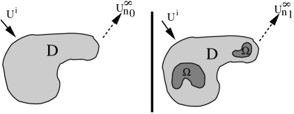
Figure 1: Reference setting (left) and actual setting (right).

We consider an inverse scattering problem consisting in shape reconstruction from physical measurements. These problems are generally non-linear and ill-posed. More specifically, we address the problem of reconstructing the support of a perturbation in a given inhomogeneous background medium from acoustic far-field measurements generated with plane waves. It may indeed happen that, in some places, the actual index is different from the reference value, as seen in Figure 1. This could happen for instance from a deterioration or an incorrect estimation of the actual index. We then say that there is a defect at any point where the reference index is different from the actual index.

A wide range of methods achieve the localization of obstacles by a sampling approach: the points of the unknown domain are characterized by a binary test that has to be applied to the whole space. For most of them, the first formulation of this pointwise test is to check if some well chosen test-function is in the range of an implicitly defined operator. See [4, 15] and references therein for a topical review. A natural way to proceed is then to connect the range of the implicit operator to the range of an operator explicitly defined from the actually available measurements. This is the principle of the linear sampling method [5, 7, 3] or of the factorization method [9, 12, 1]. Yet, when looking for perturbations in non-homogeneous background media, it is only recently that a factorization method has been proposed to reconstruct the shape of defects [14, 8].

However, we investigate in this paper an optimization approach in the lines of the inf criterion [11] to deal with the implicit operator’s range. We show that this leads to a characterization of the defects as the support of the following function:

$$\mathcal{M}_{W}(z)\mathrel{:}=\inf\left\{f_{W}(\Psi),\ \Psi\in L^{2}(S^{d-1})\text{ and }{\left\langle\Psi,\,\overline{u_{n_{0}}(\cdot,z)}\right\rangle}_{L^{2}(S^{d-1})}=1\right\},$$

where $u_{n_{0}}$ is the total field for the reference index and the form $f_{W}$ is given by

$$f_{W}(\Psi)\mathrel{:}=\left\lvert\left\langle W\Psi,\,\Psi\right\rangle_{L^{2}(S^{d-1})}\right\rvert^{\frac{1}{2}},$$

with a measurements operator $W$ explicitly built from the available data. Throughout this paper, $\left\langle\cdot,\,\cdot\right\rangle_{X}$ stands for the usual hermitian inner product in the Hilbert space $H$.

This paper is structured as follows. In section 2, the mathematical setting is specified and the implicit localization of the defects is recalled. This localization is then expressed as a binary pointwise test involving an constrained optimization problem in section 3. Finally, in section 4, we investigate numerical methods for solving this optimization problem. We end by some conclusions.

2 Formal localization

If we consider time-harmonic acoustic waves with a fixed wave number $k$, the spatial part of the wave equation is modeled by the Helmholtz equation [6]. Inhomogeneous media are then represented by an acoustic refraction index, denoted by $n\in L^{\infty}(\mathbb{R}^{d})$, and so the total field, denoted by $u_{n}$, is assumed to satisfy

$$\Delta u_{n}+k^{2}n(x)u_{n}=0,\quad x\in\mathbb{R}^{d},$$ (1)

where $d$ is the problem’s dimension ($d=2$ or 3). We consider compactly supported inhomogeneities and denote by $D$ the support of $n(x)-1$. Also, we denote an incoming wave satisfying (1) with $n=1$ by $u^{i}\in L^{2}_{loc}(\mathbb{R}^{d})$. The total field is then the sum of this incoming wave and the wave scattered by the inhomogeneous medium, denoted by $u^{s}\in L^{2}_{loc}(\mathbb{R}^{d})$:

$$u_{n}\mathrel{:}=u^{s}+u^{i},$$ (2)

where the scattered wave is assumed to satisfy the Sommerfeld radiation condition

$$\partial_{r}u^{s}=iku^{s}+\mathop{}\mathopen{}{\scriptstyle\mathcal{O}}\mathopen{}\left(\left\lvert x\right\rvert^{-\frac{d-1}{2}}\right).$$ (3)

Then, the linear system (1)-(3) defines $u_{n}$ uniquely from $u^{i}$, and it is known to be invertible in $L^{2}(D)$. Thus, let us denote the corresponding automorphism by

$$\begin{array}[]{rclcl}\mathcal{T}_{n}&:&L^{2}(D)&\to&L^{2}(D),\\ &&u^{i}&\mapsto&u_{n}.\end{array}$$

Besides, the outgoing part of a wave has an asymptotic behaviour called the far field pattern, denoted by $u_{n}^{\infty}\in L^{2}(S^{d-1})$, see figure 2, and given by the Atkinson expansion [17]

$$u_{n}(x)\mathrel{:}=u^{i}(x)+\gamma\frac{e^{ik\left\lvert x\right\rvert}}{\left\lvert x\right\rvert^{\frac{d-1}{2}}}u_{n}^{\infty}(\hat{x})+\mathop{}\mathopen{}{\scriptstyle\mathcal{O}}\mathopen{}\left(\left\lvert x\right\rvert^{-\frac{d-1}{2}}\right),\quad\hat{x}\mathrel{:}=\frac{x}{\left\lvert x\right\rvert}\in S^{d-1},$$

where $\gamma$ depends only on the dimension and is defined by

$$\gamma\mathrel{:}=\begin{cases}\frac{e^{i\pi/4}}{\sqrt{8\pi k}}&\text{if }d=2,\\ \frac{1}{4\pi}&\text{if }d=3.\end{cases}$$

Figure 2: General setting and notations.

Furthermore, for practical reasons, we will mainly consider scattered waves having a plane-wave source. These plane-waves are defined by

$$u^{i}(\hat{\theta},x)\mathrel{:}=exp({ik\hat{\theta}\cdot x}),$$

where $\hat{\theta}$ is a unitary vector in $S^{d-1}$ as depicted on figure 2. Then, let us denote the total field at the point $x\in\mathbb{R}^{d}$ and with a plane-wave source of incoming direction $\hat{\theta}$, by

$${u_{n}(\hat{\theta},x)}\mathrel{:}=\mathcal{T}_{n}(u^{i}(\hat{\theta},\cdot))(x).$$

The corresponding far-field pattern in the measurement direction $\hat{x}\in S^{d-1}$ will be denoted by $u_{n}^{\infty}(\hat{\theta},\hat{x})$. Lastly, these measurements will be used in the form of the classical far-field operator $F_{n}:L^{2}(S^{d-1})\to L^{2}(S^{d-1})$, defined by

$$F_{n}g(\hat{x})\mathrel{:}=\left\langle g,\,\overline{u_{n}^{\infty}(\cdot,\hat{x})}\right\rangle_{L^{2}(S^{d-1})}.$$

We want to reconstruct the shape of defects in a reference medium whose index is denoted by $n_{0}\in L^{\infty}(D)$. Let then $n_{1}\in L^{\infty}(D)$ denote the actual index, altered by the presence of these defects. So, denote the support of the difference between the two indices (see figure 1) by

$$\Omega\mathrel{:}=\mathrm{support}(n_{1}-n_{0}).$$

Thus, the goal is to reconstruct the domain $\Omega$, through its associated characteristic function denoted $\mathbf{1}_{\Omega}$, from the reference index $n_{0}$ and far-field measurements $u_{n_{1}}^{\infty}$. Yet, it has been shown that the unknown domain can be characterized by a set of test functions and the range of some implicitly defined operator.

Theorem 1 (Implicit domain characterization).

[8, Theorem 3.2] Let us define the operator $C:L^{2}(D)\to L^{2}(S^{d-1})$ by

$$Cf(\hat{x})=\langle f,u_{n_{0}}(\hat{x},\cdot)\rangle_{L^{2}(D)}.$$

Then, for each $z\in\mathbb{R}^{d}$, we have

$$z\in\Omega\iff\overline{u_{n_{0}}(\cdot,z)}\in\mathcal{R}\left(C\mathbf{1}_{\Omega}\right),$$ (4)

where $\mathbf{1}_{\Omega}:L^{2}(\Omega)\to L^{2}(D)$ is the restriction to $\Omega$ given by

$$\mathbf{1}_{\Omega}f(\hat{x})=\begin{cases}0,\quad x\notin\Omega\\ f(x),\quad x\in\Omega\end{cases}.$$

3 Explicit identification of the defects

This section gives an explicit formulation of characterization (4). To do so, we proceed in three steps. First, we introduce a practical result formulating the belonging to the range of any given (bounded) operator $L$ as an inf criterion based on any function related to $L$ through specific assumptions. Then, we construct such a well-suited function for the operator we are interested in, namely $C\mathbf{1}_{\Omega}$. Finally, we can give the explicit characterization of the defect $\Omega$.

3.1 Formulation of a bounded operator’s range through an inf criterion

To deal with the range of $C\mathbf{1}_{\Omega}$, depending on the unknown domain $\Omega$, let us recall the following characterization of an operator’s range.

Lemma 2 (Range characterization).

[14, Lemma 2.1] Let $L:H_{1}\to H_{2}$ be a bounded operator between two Hilbert spaces $H_{1}$ and $H_{2}$, and let $\varphi\in H_{2}$. Then, noting $H_{2}^{\star}$ the dual of $H_{2}$ and identifying $H_{1}$ with its dual, $\varphi\in\mathcal{R}\left(L\right)$ if and only if there exists $c>0$ such that for all $\Psi\in H_{2}^{\star}$

$$\left\lvert\left\langle\Psi,\,\varphi\right\rangle\right\rvert\leqslant c\left\lVert L^{\star}\Psi\right\rVert.$$ (5)

Hence, any form comparable to $\left\lVert L^{\star}(\cdot)\right\rVert$ can be used to characterize the range of the operator $L$.

Corollary 3.

With $L$ as in lemma 2, let $f:H_{2}^{\star}\to\mathbb{R}$ be comparable to $L^{\star}$ in the sense that there exists $c_{1}>0$ and $c_{2}>0$ such that

$$c_{1}\left\lVert L^{\star}\Psi\right\rVert\leqslant f(\Psi)\leqslant c_{2}\left\lVert L^{\star}\Psi\right\rVert,\quad\Psi\in H_{2}^{\star}.$$ (6)

Then, $\varphi\in\mathcal{R}\left(L\right)$ if and only if there exists $c_{3}>0$ such that for all $\Psi\in H_{2}^{\star}$

$$\left\lvert\left\langle\Psi,\,\varphi\right\rangle\right\rvert\leqslant c_{3}f(\Psi).$$ (7)

Proof. The result (7) is a straightforward combination of the characterization (5) and (6). ∎ Finally, from corollary 3, we deduce the following characterization based on an inf criterion.

Corollary 4.

With $f$ as in corollary 3, then $\varphi\in\mathcal{R}\left(L\right)$ if and only if

$$0<\inf\left\{f(\Psi),\ \Psi\in H_{2}^{\star}\text{ and }{\left\langle\Psi,\,\varphi\right\rangle}=1\right\}.$$

Proof. First, if $\varphi\not\in\mathcal{R}\left(L\right)$, from corollary 3, for each $c>0$ there exists $\Psi_{c}\in H_{2}^{\star}$ such that $\left\lvert\left\langle\Psi_{c},\,\varphi\right\rangle\right\rvert>cf(\Psi_{c}).$ Since $f(\Psi_{c})\geqslant 0$ by (6), then ${\left\langle\Psi_{c},\,\varphi\right\rangle}\not=0$ and we can define $\psi_{c}\mathrel{:}=\Psi_{c}/{\left\langle\Psi_{c},\,\varphi\right\rangle}$. From (6), it follows

$$1=\left\lvert\left\langle\Psi_{c},\,\varphi\right\rangle\right\rvert\frac{1}{\left\lvert\left\langle\Psi_{c},\,\varphi\right\rangle\right\rvert}>cf(\Psi_{c})\frac{1}{\left\lvert\left\langle\Psi_{c},\,\varphi\right\rangle\right\rvert}\geqslant cf(\psi_{c})\frac{c_{1}}{c_{2}}.$$

So, there is a set of functions $\psi_{c}\in H_{2}^{\star}$, satisfying ${\left\langle\psi_{c},\,\varphi\right\rangle}=1$, such that $f(\psi_{c})\to 0$ when $c\to\infty$.

Next, let $\varphi\in H_{2}\setminus\{0\}$ be in the range of the operator $L$ and let $\Psi\in H_{2}^{\star}$ satisfy $\left\langle\Psi,\,\varphi\right\rangle=1$. Thus, from corollary 3, there exists $c_{3}>0$ such that $1\leqslant c_{3}f(\Psi)$ and the infimum is not vanishing. Finally, if $\varphi=0$, which is always in the range of $L$, the infimum is evaluated over an empty set and will then conventionally be given the value $+\infty$. ∎

3.2 Construction of a well-suited objective function

As shown in corollary 4, the range of a linear bounded operator $L$ can be formulated as a usual constrained optimization problem without the exact knowledge of $L$. Indeed, it suffices to find any form $f$ satisfying (6). Hence, to get an explicit characterization of the domain $\Omega$ from theorem 1, we look for a form $f$ satisfying

$$c_{1}\left\lVert\mathbf{1}_{\Omega}C^{\star}\Psi\right\rVert\leqslant f(\Psi)\leqslant c_{2}\left\lVert\mathbf{1}_{\Omega}C^{\star}\Psi\right\rVert,\quad\Psi\in L^{2}(S^{d-1}).$$ (8)

To achieve this, following [11], we consider the form $f_{W}:L^{2}(S^{d-1})\to\mathbb{R}_{+}$ defined by

$$f_{W}(\Psi)\mathrel{:}=\left\lvert\left\langle W\Psi,\,\Psi\right\rangle_{L^{2}(S^{d-1})}\right\rvert^{\frac{1}{2}},$$ (9)

where $W$ is a measurements operator explicitly built from the available data.

A first guess for the operator $W$ would be to consider $(F_{n_{1}}-F_{n_{0}})$: the difference between the far-field operators corresponding respectively to the reference index $n_{0}$ and the actual index $n_{1}$. But it has been shown in [8] that this subtraction does not yield some crucial factorization. Thus, we have to restrain ourselves to full bi-static data ($u_{n_{0}}^{\infty}$ and $u_{n_{1}}^{\infty}$ are known over $S^{d-1}\times S^{d-1}$) and non-absorbing media ($n_{0}(x)$ and $n_{1}(x)\in\mathbb{R}$) so we can consider the operator $W:L^{2}(S^{d-1})\to L^{2}(S^{d-1})$ defined by

$$W\mathrel{:}=\left(\mathrm{id}+2ik\left\lvert\gamma\right\rvert^{2}F_{n_{0}}\right)\left(F_{n_{1}}-F_{n_{0}}\right).$$

Under these assumptions, it has been shown that this measurements operator $W$ has a factorization of the form (see [8, Corollary 4.7, Corollary 4.3])

$$W=CAC^{\star},$$ (10)

where the operator $A$ is an automorphism on $L^{2}(\Omega)$ defined by

$$A\mathrel{:}=\mathbf{1}_{\Omega}k^{2}(n_{1}-n_{0})\mathcal{T}_{n_{1}}\mathcal{T}_{n_{0}}^{-1}\mathbf{1}_{\Omega}.$$ (11)

So, we have

$$f_{W}(\Psi)=\left\lvert\left\langle CAC^{\star}\Psi,\,\Psi\right\rangle_{L^{2}(S^{d-1})}\right\rvert^{\frac{1}{2}}=\left\lvert\left\langle AC^{\star}\Psi,\,C^{\star}\Psi\right\rangle_{L^{2}(\Omega)}\right\rvert^{\frac{1}{2}},$$ (12)

and as such, the inequalities (8) are then the continuity and the coercivity of the operator $A$, at least on the range of $C^{\star}$. We are now going to show that this coercivity is related to the contrast between the reference index $n_{0}$ and the actual values of $n_{1}$, i.e. the defects should be clearly distinguished from the background. We thus make the following geometrical assumption.

Assumption 5.

Assume that $n_{0}$ and $n_{1}$ are real valued and that either $(n_{1}-n_{0})$ or $(n_{0}-n_{1})$ is locally bounded from below:

• for any compact subset $\omega$ included in $\Omega$, there exists $c>0$ such that $(n_{1}(z)-n_{0}(z))\geqslant c$ for almost all $z\in\omega$,

or

• for any compact subset $\omega$ included in $\Omega$, there exists $c>0$ such that $(n_{0}(z)-n_{1}(z))\geqslant c$ for almost all $z\in\omega$.

Moreover, for a fixed geometry of defects, some wave numbers $k$ may produce resonances that cancel the outgoing wave. Indeed, the operator mapping an incoming wave to the corresponding far-field pattern is not one-to-one in the case of inhomogeneous media. This corresponds to the so-called interior transmission eigenvalues arise [10].

Definition 6.

We call $k$ an interior transmission eigenvalue for the pair of indices $(n_{0},n_{1})$ if there exists a non-vanishing (source,solution) pair, denoted by $(h,u)\in\left(L^{2}(\Omega)\right)^{2}$, such that

$$\left\{\begin{aligned} (\Delta+k^{2}n_{0})u&=-k^{2}(n_{1}-n_{0})h\text{ in }\Omega,\\ (\Delta+k^{2}n_{1})h&=0\text{ in }\Omega,\\ u&=0\text{ on }\partial\Omega,\\ \partial_{\nu}u&=0\text{ on }\partial\Omega.\\ \end{aligned}\right.$$

Since we want to avoid these ”pathological” values, it is useful to know that this is a rare case.

Lemma 7.

If the indices $n_{0}$ and $n_{1}$ are real-valued, then the set of interior transmission eigenvalue for the pair of indices $(n_{0},n_{1})$ is discrete. Furthermore, if there are infinitely many, they only accumulate at $+\infty$.

Proof. The proof follows exactly the lines of [13, Theorems 4.13 and 4.14], by adapting the notations. ∎ With these two geometrical restrictions, the coercivity of the operator $A$ on the range of $C^{\star}$ is then obtained in lemma 9, using the following result.

Lemma 8.

[13, Lemma 1.17] Let $Y$ be a subset of a reflexive Banach space $X$ and $A$, $A_{0}$ : $X^{\star}\to X$ be linear and bounded operators such that

1. $\left\langle\varphi,\,A\varphi\right\rangle\in\mathbb{C}\setminus(-\infty,0]$ for all $\varphi\neq 0$ in the closure of $Y$

2. $\left\langle\varphi,\,A_{0}\varphi\right\rangle\in\mathbb{R}$ and there exists $c_{0}>0$ with $\left\langle\varphi,\,A_{0}\varphi\right\rangle\geqslant c_{0}\left\lVert\varphi\right\rVert$ for all $\varphi$ in $Y$

3. $A-A_{0}$ is compact.

Then, there exists $c>0$ such that for all $\varphi\in Y$ it holds $\left\lvert\left\langle A\varphi,\,\varphi\right\rangle\right\rvert\geqslant c\left\lVert\varphi\right\rVert^{2}_{X^{\star}}.$

Finally, we group the properties of operator $A$ in the following lemma.

Lemma 9.

Under assumption 5, if $k$ is not an interior transmission eigenvalue in the sense of definition 6, then the operator $A$, defined by (11), is coercive on the range of $C^{\star}$, defined in theorem 1. Namely, there exists $c_{1}>0$ such that

$$c_{1}\left\lVert\mathbf{1}_{\Omega}C^{\star}\Psi\right\rVert_{L^{2}(\Omega)}\leqslant\left\lvert\left\langle AC^{\star}\Psi,\,C^{\star}\Psi\right\rangle_{L^{2}(\Omega)}\right\rvert^{\frac{1}{2}},\ \forall\Psi\in L^{2}(S^{d-1}).$$ (13)

Proof. This is a straightforward application of lemma 8 with $Y=\mathcal{R}\left(C^{\star}\right)$ and $X=L^{2}(\Omega)$. The required assumptions have been partially shown [8, lemma 5.3] but, for convenience, we give a complete proof.

1. Choose $\varphi\in\mathcal{R}\left(C^{\star}\right)$. By definition of operator $C$, this is a total field for the refraction index $n_{0}$. Hence, there exists an incident field $f$ such that $\varphi=\mathcal{T}_{n_{0}}(f)$. Let us set $u_{n_{0}}=\varphi$ and $u_{n_{1}}=\mathcal{T}_{n_{1}}(f)$. Thus, we obtain $A\varphi=k^{2}(n_{1}-n_{0})u_{n_{1}}$. Moreover, choosing $R>0$ such that the ball $B_{R}$ of radius $R$ contains $\Omega$, it holds that

   $$\int_{\Omega}k^{2}(n_{1}-n_{0})u_{n_{1}}(\overline{u_{n_{0}}-u_{n_{1}}})$$

   $$=\int_{B_{R}}(\Delta+k^{2}n_{0})(u_{n_{1}}-u_{n_{0}})(\overline{u_{n_{1}}-u_{n_{0}}})$$

   $$=\int_{B_{R}}k^{2}n_{0}|u_{n_{1}}-u_{n_{0}}|^{2}-|\nabla(u_{n_{1}}-u_{n_{0}})|^{2}+\int_{S_{R}}(\overline{u_{n_{1}}-u_{n_{0}}})\partial_{\nu}(u_{n_{1}}-u_{n_{0}}).$$

   By letting $R$ go to infinity, it comes

   $$\int_{\Omega}k^{2}(n_{1}-n_{0})u_{n_{1}}(\overline{u_{n_{0}}-u_{n_{1}}})$$

   $$=\int_{\mathbb{R}^{n}}k^{2}n_{0}|u_{n_{1}}-u_{n_{0}}|^{2}-|\nabla(u_{n_{1}}-u_{n_{0}})|^{2}+ik\left\lvert\gamma\right\rvert^{2}\int_{S^{d-1}}|u_{n_{1}}^{\infty}-u_{n_{0}}^{\infty}|^{2}.$$

   Hence, taking the imaginary part yields

   $$Im\int_{\Omega}k^{2}(n_{1}-n_{0})u_{n_{1}}\overline{u_{n_{0}}}=k\left\lvert\gamma\right\rvert^{2}\int_{S^{d-1}}|u_{n_{1}}^{\infty}-u_{n_{0}}^{\infty}|^{2}.$$

   This shows that $Im\langle A\varphi,\varphi\rangle\geqslant 0$ and if this quantity is vanishing, we deduce that $u_{n_{1}}^{\infty}=u_{n_{0}}^{\infty}$. Moreover, out of $\Omega$ we have

   $$(\Delta+k^{2}n_{0})u_{n_{0}}=(\Delta+k^{2}n_{1})u_{n_{1}}=(\Delta+k^{2}n_{0})u_{n_{1}}.$$

   As a consequence, the unique continuation principle [6, theorem 8.6] yields $u_{n_{1}}=u_{n_{0}}$ out of $\Omega$. So, the quantity $w\mathrel{:}=(u_{n_{1}}-u_{n_{0}})$ has its support included in $\Omega$ and satisfies $(\Delta+k^{2}n_{0})w=-(n_{1}-n_{0})u_{n_{1}}$. If $k$ is not a transmission eigenvalue, we then have $w=0$ and $u_{n_{1}}\displaystyle\left|{}_{\Omega}\right.=0$. Finally, this implies that $u_{n_{1}}=0$ by the unique continuation principle and all these results are extended to $\overline{\mathcal{R}\left(C^{\star}\right)}$ by continuity to prove item 1.

2. Furthermore, we also have that

   $$\langle A\varphi,\varphi\rangle =\int_{\Omega}k^{2}(n_{1}-n_{0})|u_{n_{0}}|^{2}+\int_{\Omega}k^{2}(n_{1}-n_{0})(u_{n_{1}}-u_{n_{0}})\overline{u_{n_{0}}}$$

   $$=\langle A_{0}\varphi,\varphi\rangle+\langle K\varphi,\varphi\rangle,$$

   with $A_{0}=k^{2}(n_{1}-n_{0})I$ and $K=k^{2}(n_{1}-n_{0})(\mathcal{T}_{n_{1}}\mathcal{T}_{n_{0}}^{-1}-I)$. Under assumption 5, $A_{0}$ is clearly coercive and self-adjoint.

3. Moreover, $K=k^{2}(n_{1}-n_{0})(\mathcal{T}_{n_{1}}-\mathcal{T}_{n_{0}})\mathcal{T}_{n_{0}}^{-1}$. Yet, it is known from the Lippmann-Schwinger equation [6, equation (8.12)] that $\mathcal{T}_{n}=id-T\mathcal{T}_{n}$, where $T$ is some compact operator. Thus, $(\mathcal{T}_{n_{1}}-\mathcal{T}_{n_{0}})$ is compact, and so is $K$.

∎

3.3 Characterization of the defects from the measurements

We are now able to state an explicit localization of the defects in the form of a constrained optimization problem that extends the characterization proposed in [11].

Theorem 10.

Assume that $k$ is not an interior transmission eigenvalue for the indices $n_{0}$ et $n_{1}$, following definition 6, that these indices are contrasted following assumption 5 and that we have full bi-static data (i.e. $u_{n_{0}}^{\infty}$ and $u_{n_{1}}^{\infty}$ are known over $S^{d-1}\times S^{d-1}$).

We can then define the value

$$\mathcal{M}_{W}(z)\mathrel{:}=\inf\left\{f_{W}(\Psi),\ \Psi\in L^{2}(S^{d-1})\text{ and }{\left\langle\Psi,\,\overline{u_{n_{0}}(\cdot,z)}\right\rangle}_{L^{2}(S^{d-1})}=1\right\},$$ (14)

and for each point $z\in\mathbb{R}^{d}$ we have

$$z\in\Omega\iff\mathcal{M}_{W}(z)>0.$$ (15)

Proof. Theorem 1 characterizes the domain of the defects $\Omega$ by

$$z\in\Omega\iff\overline{u_{n_{0}}(\cdot,z)}\in\mathcal{R}\left(C\mathbf{1}_{\Omega}\right).$$

The result (15) is then a direct consequence of corollary 4 with $f=f_{W}$, $\varphi=\overline{u_{n_{0}}(\cdot,z)}$, $L=C\mathbf{1}_{\Omega}$ and $H_{2}=L^{2}(S^{d-1})$. So what is left to prove is that the double inequality (8) holds. Now, we deduce from (12) that the right inequality comes from the boundedness of the operator $A$. The left one was established in lemma 9. ∎

4 Numerical methods for the computation of the infimum’s value

In theorem 10, we have expressed the localization of the defects as a pointwise binary test, taking the form of a constrained optimization problem. We are now interested in the numerical computation of the values of the function $\mathcal{M}_{W}(z)$ defined in (14). We thus explicit, and then test, two usual minimization algorithms working on this problem: the steepest descent and the gradient projection.

4.1 Algorithms

Both minimization methods we are going to use require explicit gradients of the cost function. To simplify their expression, we will consider the minimization of the following form on $L^{2}(S^{d-1})$, defined for any $\Psi$ by

$$f_{W}^{4}(\Psi)\mathrel{:}=\big{(}f_{W}(\Psi)\big{)}^{4}=\left\lvert\left\langle W\Psi,\,\Psi\right\rangle_{L^{2}(S^{d-1})}\right\rvert^{2}.$$

Since we only want to know if the infimum is vanishing, this gives results equivalent to (14) and we thus have to evaluate

$$\big{(}\mathcal{M}_{W}(z)\big{)}^{4}\mathrel{:}=\inf\left\{f_{W}^{4}(\Psi),\ \Psi\in L^{2}(S^{d-1})\text{ and }{\left\langle\Psi,\,\overline{u_{n_{0}}(\cdot,z)}\right\rangle}_{L^{2}(S^{d-1})}=1\right\}.$$ (16)

Remark 11.

The function $\mathcal{M}_{W}(z)$ has been proved to vanish outside of the defects and yet, it can be seen that the value 0 can never be attained while satisfying the constraint.

To show this, let $\Psi_{\star}\in L^{2}(S^{d-1})$ be such that $f_{W}^{4}(\Psi_{\star})=0$. Then, from factorization (10) and inequalities (13), it holds that $f_{W}^{4}(\Psi_{\star})=\left\langle AC^{\star}\Psi_{\star},\,C^{\star}\Psi_{\star}\right\rangle^{2}\geqslant\left\lVert\mathbf{1}_{\Omega}C^{\star}\Psi_{\star}\right\rVert^{4}$, that is $C^{\star}{\Psi_{\star}}\displaystyle\left|{}_{\Omega}\right.=0$. Furthermore, it is easy to see that $C^{\star}{\Psi_{\star}}$ satisfies the Helmholtz equation (1) on $\mathbb{R}^{d}$ with $n=n_{0}$. The unique continuation principle then yields $C^{\star}{\Psi_{\star}}=0$, and thus ${\Psi_{\star}}=0$ by injectivity of $C^{\star}$, which has been shown in the proof of [8, Proposition 5.4]. As a consequence, $\Psi_{\star}$ can not satisfy ${\left\langle\Psi_{\star},\,\overline{u_{n_{0}}(\cdot,z)}\right\rangle}=1$.

This points out that numerical approximations of a vanishing inf might be mistaken with exact non-zero inf values. Some care will thus have to be taken to set them apart, so that the plot of $\mathcal{M}_{W}(z)$ can be used to localize the defects.

We now turn to the feasible set. For $z\in\mathbb{R}^{d}$, let us denote by $\mathcal{C}_{z}$ the affine hyperplane

$$\mathcal{C}_{z}\mathrel{:}=\left\{\Psi+\frac{\overline{u_{n_{0}}(\cdot,z)}}{\left\lVert u_{n_{0}}(\cdot,z)\right\rVert^{2}},\ \Psi\in L^{2}(S^{d-1}),\ \left\langle\Psi,\,\overline{u_{n_{0}}(\cdot,z)}\right\rangle_{L^{2}(S^{d-1})}=0\right\}.$$

The orthogonal projection on $\mathcal{C}_{z}$, denoted by $P_{\mathcal{C}_{z}}$, is defined on $L^{2}(S^{d-1})$ by the affine mapping

$$P_{\mathcal{C}_{z}}\Psi\mathrel{:}=\Psi-\frac{\left\langle\Psi,\,\overline{u_{n_{0}}(\cdot,z)}\right\rangle}{\left\lVert u_{n_{0}}(\cdot,z)\right\rVert^{2}}\overline{u_{n_{0}}(\cdot,z)}+\frac{\overline{u_{n_{0}}(\cdot,z)}}{\left\lVert u_{n_{0}}(\cdot,z)\right\rVert^{2}}.$$ (17)

Hence, finding an infimum of $f_{W}^{4}$ over $\mathcal{C}_{z}$ is equivalent to looking for the infimum over $L^{2}(S^{d-1})$ of

$$P_{f_{W}^{4}}\mathrel{:}=f_{W}^{4}\circ P_{\mathcal{C}_{z}}.$$

We can therefore compute a minimizing sequence $x_{n}$ for the form $P_{f_{W}^{4}}$ by any unconstrained optimization method. For convenience, all gradients and hessians are calculated in section A.1 and their finite dimension formulation is given in section A.2. It then follows from theorem 10 that if $\big{(}P_{f_{W}^{4}}(x_{n})\big{)}_{n}$ goes to 0, the point $z$ is outside $\Omega$, and inside otherwise. A basic example of descent is presented in algorithm 1:

Input: $x_{0}$ chosen in $L^{2}(S^{d-1})$

repeat

       Compute $\alpha_{n}$ such that $P_{f_{W}^{4}}(x_{n}-\alpha_{n}\nabla P_{f_{W}^{4}}(x_{n}))<P_{f_{W}^{4}}(x_{n})$;

       Update $x_{n+1}\leftarrow x_{n}-\alpha_{n}\nabla P_{f_{W}^{4}}(x_{n})$;

until $\left\lVert x_{n+1}-x_{n}\right\rVert/(1+\left\lVert x_{n}\right\rVert)<\varepsilon$;

Output: $P_{f_{W}^{4}}(x_{N})$

Algorithm 1 Steepest descent

Moreover, since the projection on $\mathcal{C}_{z}$ is easy to write, we can also consider a gradient projection method [16]. As previously, if $\big{(}f_{W}^{4}(x_{n})\big{)}_{n}$ goes to 0, the point $z$ is outside $\Omega$. The principle of the gradient projection is presented in algorithm 2:

Input: $x_{0}$ chosen in $\mathcal{C}_{z}$

repeat

       Compute $\alpha_{n}$ such that $f_{W}^{4}(x_{n}-\alpha_{n}\nabla f_{W}^{4}(x_{n}))<f_{W}^{4}(x_{n})$;

       Project and update $x_{n+1}\leftarrow P_{\mathcal{C}_{z}}(x_{n}-\alpha_{n}\nabla f_{W}^{4}(x_{n}))$;

until $\left\lVert x_{n+1}-x_{n}\right\rVert/(1+\left\lVert x_{n}\right\rVert)<\varepsilon$;

Output: $f_{W}^{4}(x_{N})$

Algorithm 2 Gradient projection

Remark 12.

Since the projector $P_{\mathcal{C}_{z}}$ is an affine map, the proposed steepest descent and gradient projection methods are very close. Indeed, we note that by choosing a constant descent step $\alpha_{n}=\alpha$ and a starting point $x_{0}\in\mathcal{C}_{z}$, both algorithms define the same sequence. The computation of $\alpha_{n}$ is however done before the projection in algorithm 2, and after it in algorithm 1. Thus, the values coming up for $\alpha_{n}$ in each of the proposed algorithms will seemingly be different and produce different sequences $x_{n}$.

4.2 Numerical validation on a simple case

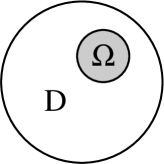
Figure 3: A simple study case

We present here some 2D numerical results in the simple case illustrated on figure 3. The considered object of support is a disc $D$ of section 2.1 containing defects which are also in the shape of a disc $\Omega$ of section 0.6. With a fixed wave number $k=10$, the size of the object is then thrice the wavelength and the size of the defects is approximatively one wavelength. Also, the reference index $n_{0}$ takes its values in $[1.56,\,1.84]$ inside $D$ and the perturbed version $n_{1}$ takes its values in $[2.01,\,2.16]$ inside $\Omega$. Finally, we used $99$ incoming/measurement directions evenly distributed over $[0,\,2\pi]$.

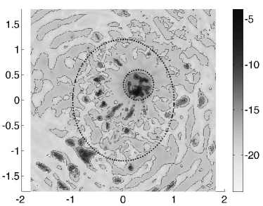
(a) Steepest descent algorithm

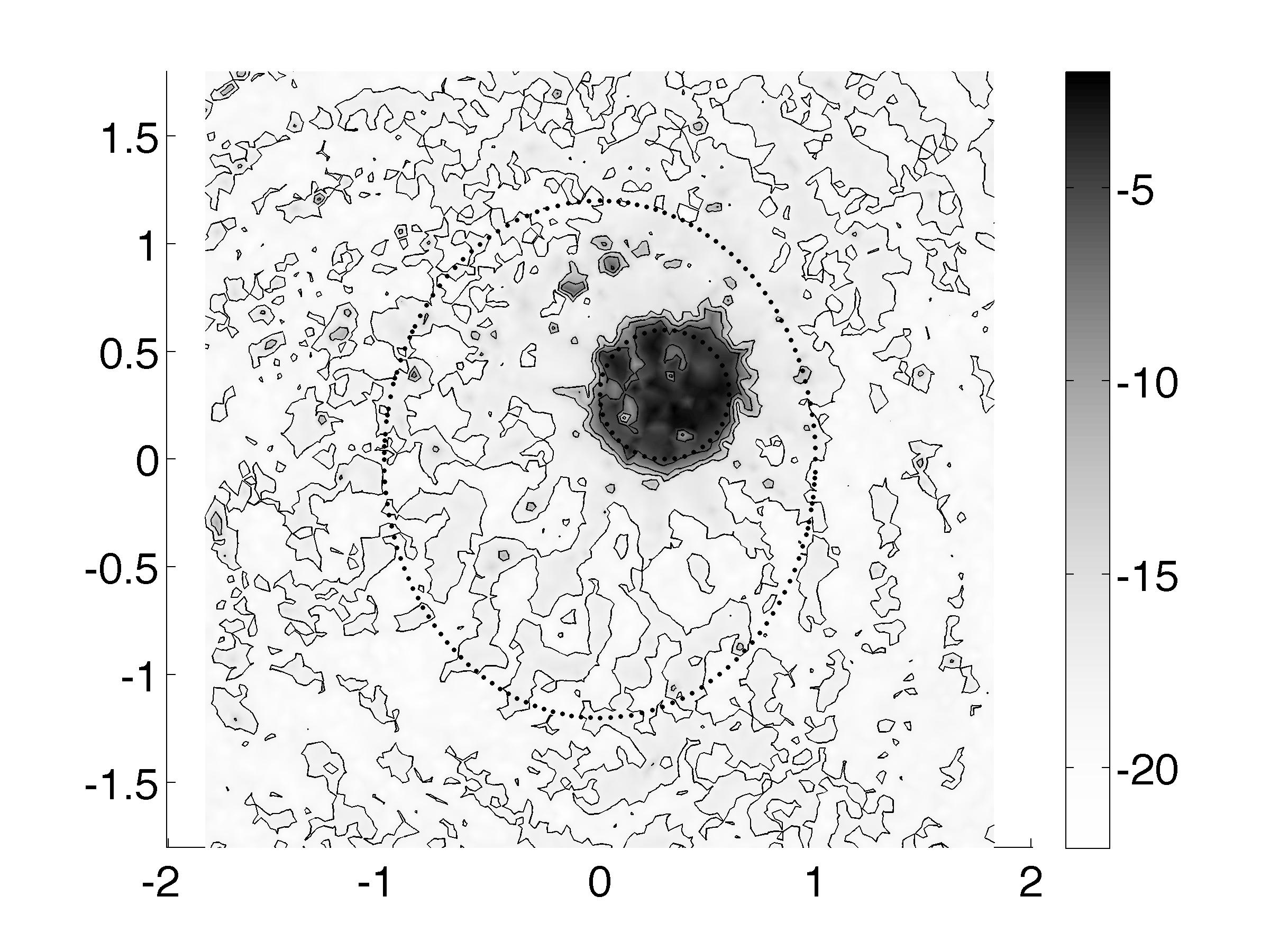
(b) Gradient projection algorithm

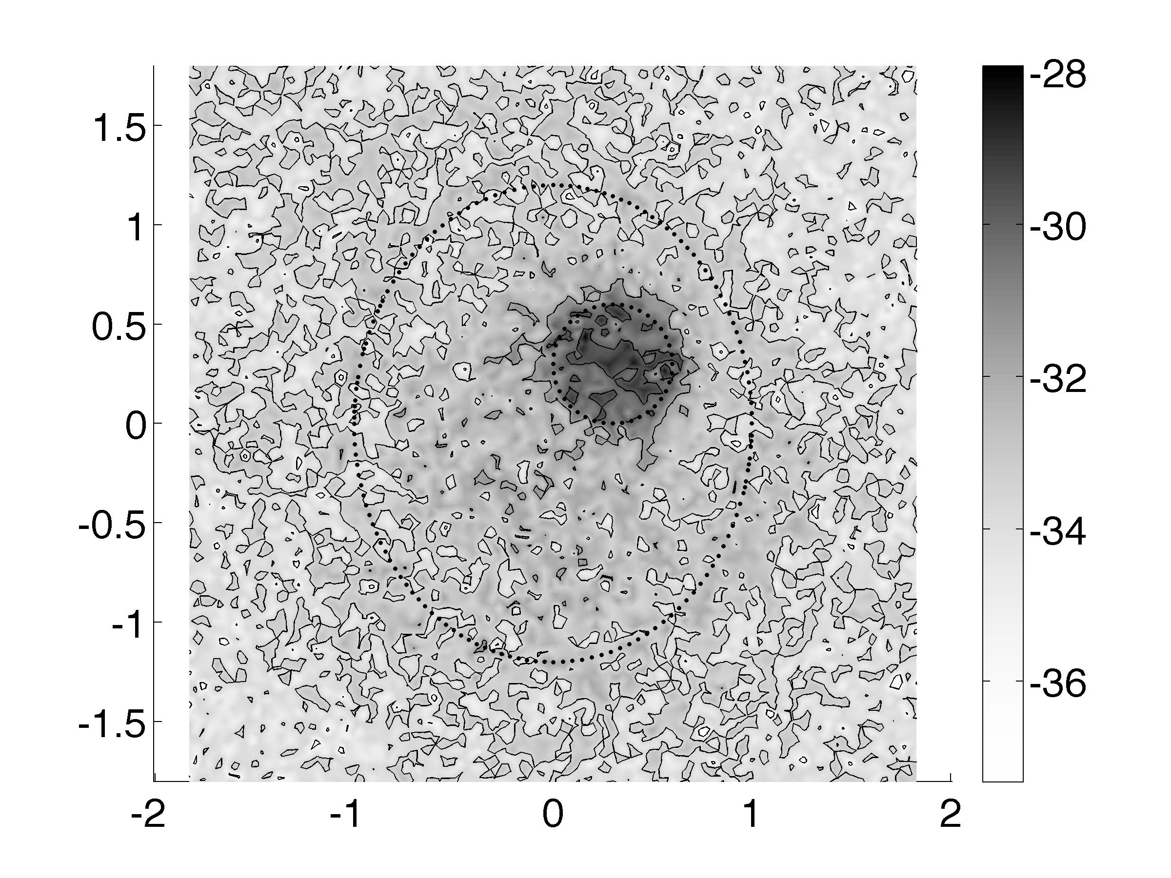
(c) Matlab’s fminunc function

(d) Matlab’s fmincon function

Number of iterations	min	med	max ($\leqslant 400$)
Steepest descent	11	400	400
Gradient projection	14	120	400
Matlab’s fminunc function	8	17	68
Matlab’s fmincon function	9	19	58

Figure 4: Values of $\log_{10}\mathcal{M}_{W}(z)$ computed by various optimization methods with a relative tolerance on $x_{n}$ set to $10^{-9}$ as the only stopping rule

Figure 4 displays the infimums’s values $\big{(}\mathcal{M}_{W}(z)\big{)}^{4}$ in a $\log_{10}$ scale, respectively obtained for each sampling point $z_{i}$ (about 8500) with algorithm 1 (figure 4a) and algorithm 2 (figure 4b). Note that these sampling points are unrelated to the finite elements nodes that were used to generate the data. The linear search for the step length $\alpha$ was done by simple dichotomy on the gradient. We also present the results obtained with Matlab’s fminunc function applied to the form $P_{f_{W}^{4}}$ (figure 4c) and Matlab’s fmincon function applied to the form $f_{W}^{4}$ over the feasible set $\mathcal{C}_{z_{i}}$ (figure 4d). The fminunc and fmincon functions are based on the interior-reflective Newton method described in [2]. Furthermore, for each sampling point and each algorithm, the sequence has been initialized by $x_{0}=P_{\mathcal{C}_{z_{i}}}(0)={\overline{u_{n_{0}}(\cdot,z_{i})}}/{\left\lVert u_{n_{0}}(\cdot,z_{i})\right\rVert^{2}}\in\mathcal{C}_{z_{i}}$. Indeed, it seems natural to start with a point already satisfying the constraint.

As can be expected, Matlab’s functions give much faster results, but we note that even the very basic algorithms we proposed yield acceptable results. This shows that the iterative optimization approach resulting in theorem 10 can produce a satisfactory localization of the defects, but for a computational cost that is not controlled at this point.

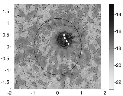
(a) Steepest descent algorithm

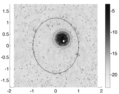
(b) Gradient projection algorithm

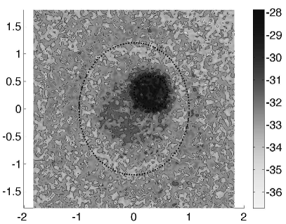
(c) Matlab’s fminunc function

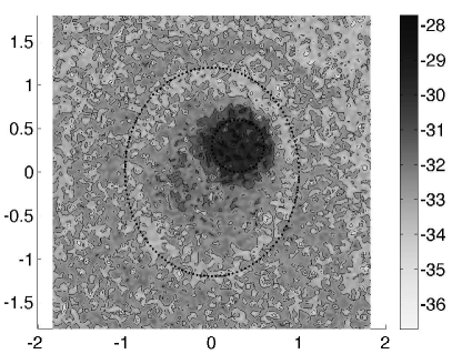
(d) Matlab’s fmincon function

Number of iterations	min	med	max ($\leqslant 400$)
Steepest descent	5	10	400
Gradient projection	6	12	145
Matlab’s fminunc function	6	10	14
Matlab’s fmincon function	8	12	18

Figure 5: Values of $\log_{10}\mathcal{M}_{W}(z)$ with $10\%$ uniform noise added to the measurements

To go further, we also tested the sensitivity with respect to the data, to take into account simulation or measurement inaccuracy. This was done by adding uniform random noise to the measurements and thus, using $u^{\varepsilon}_{n_{1}}$ such that $\left\lVert u^{\varepsilon}_{n_{1}}-u^{\infty}_{n_{1}}\right\rVert<\varepsilon\left\lVert u^{\infty}_{n_{1}}\right\rVert$. The optimization approach turns out to be quite robust regarding this criterion. Indeed, figure 5 shows that acceptable results are still obtained with $10\%$ relative noise, with a seemingly better visualization for the gradient projection algorithm. As this is sometimes the case, we also note that adding some noise has a slightly regularizing effect that visibly enhances convergence speed for the basic algorithms 1 and 2.

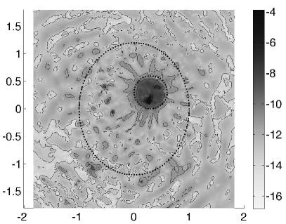
(a) Steepest descent algorithm

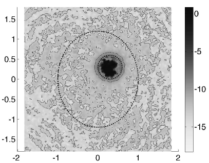
(b) Gradient projection algorithm

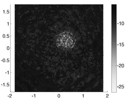
(c) Matlab’s fminunc function

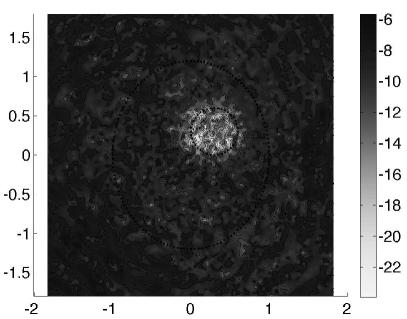
(d) Matlab’s fmincon function

Number of iterations	min	med	max ($\leqslant 400$)
Steepest descent	4	46	400
Gradient projection	5	29	400
Matlab’s fminunc function	4	9	23
Matlab’s fmincon function	7	9	26

Figure 6: Localization of the defects with the relative tolerances set to $10^{-6}$

Remark 13.

The results in figures 4 and 5 were obtained by considering only the relative variation on $x_{n}$, as proposed in algorithm 1: $\left\lVert x_{n+1}-x_{n}\right\rVert/(1+\left\lVert x_{n}\right\rVert)<10^{-9}.$ Yet, many optimization algorithms rely on multiple stopping criterions, including a relative variation tolerance with respect to the cost function’s values. We see here that these values are very small and thus hardly usable in a stopping rule. The same goes for the gradient and first order optimality criteria. As a consequence, we had to set the relative tolerance regarding the cost function to $10^{-32}$ in Matlab’s optimization functions, so that this condition would never be triggered. With the tolerances for the relative variation regarding $x_{n}$ and the cost function set to their default ($10^{-6}$, see Matlab’s help), we see in figure 6 that Matlab’s functions produce the opposite result to what was expected. Indeed, we see that the values of $\mathcal{M}_{W}(z)$ outside $\Omega$ are close to zero but higher than the ones inside $\Omega$. On the other hand, the simple algorithms presented in the previous section still yield the expected localizations, and at a lower computational time. This highlights that a special care has to be taken regarding the stopping rule, as we compare the minimal values issued from different minimization problems.

4.3 Experimentations on a non-trivial absorbing example

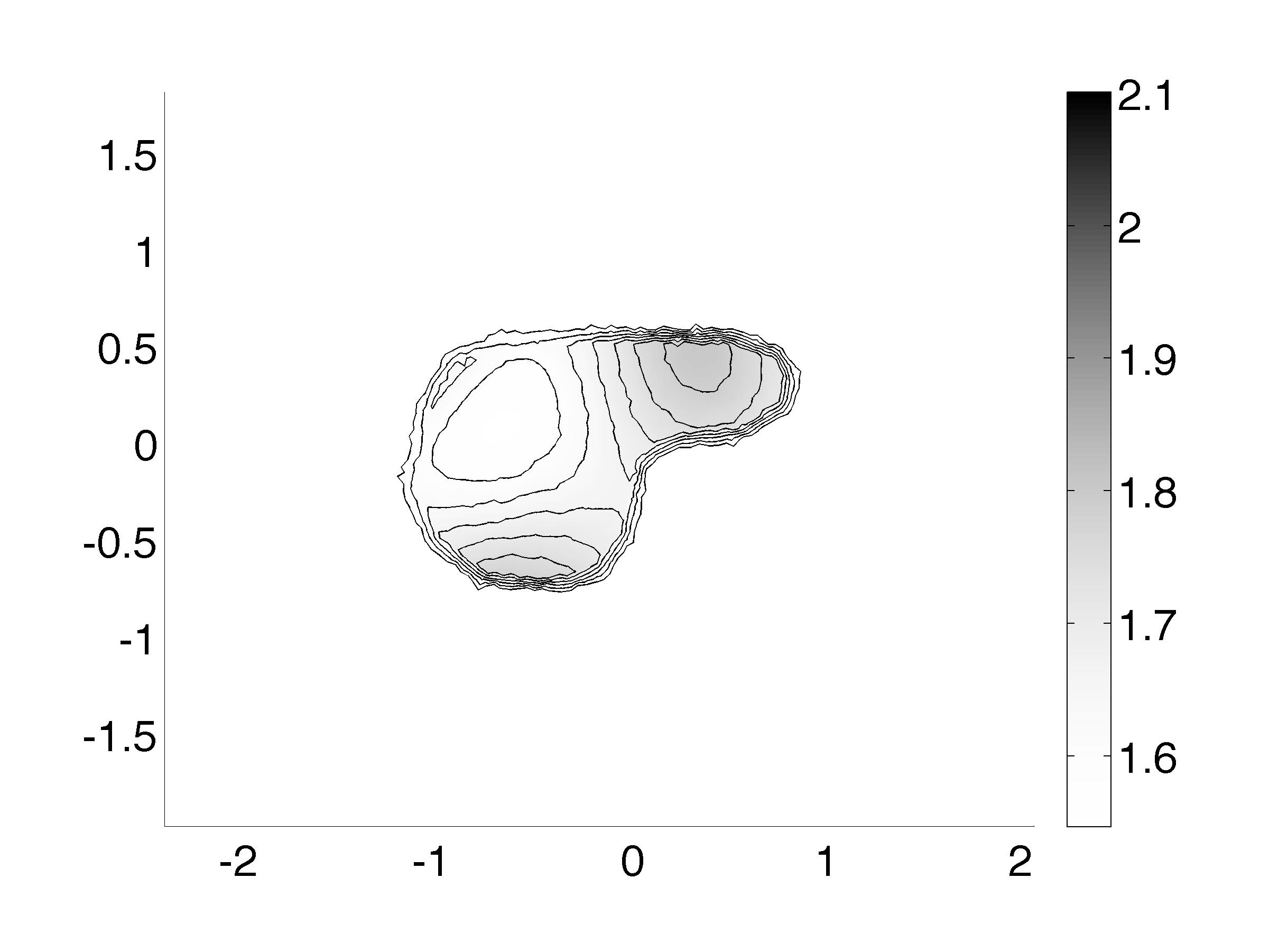
(a) Reference index’s real part

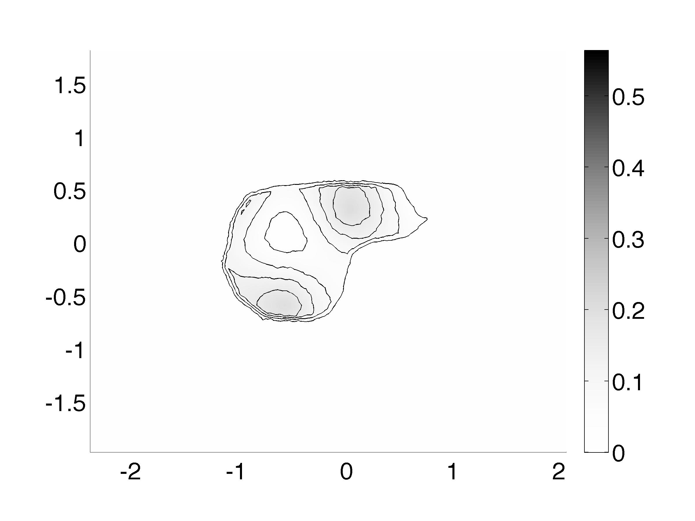
(b) Reference index’s imaginary part

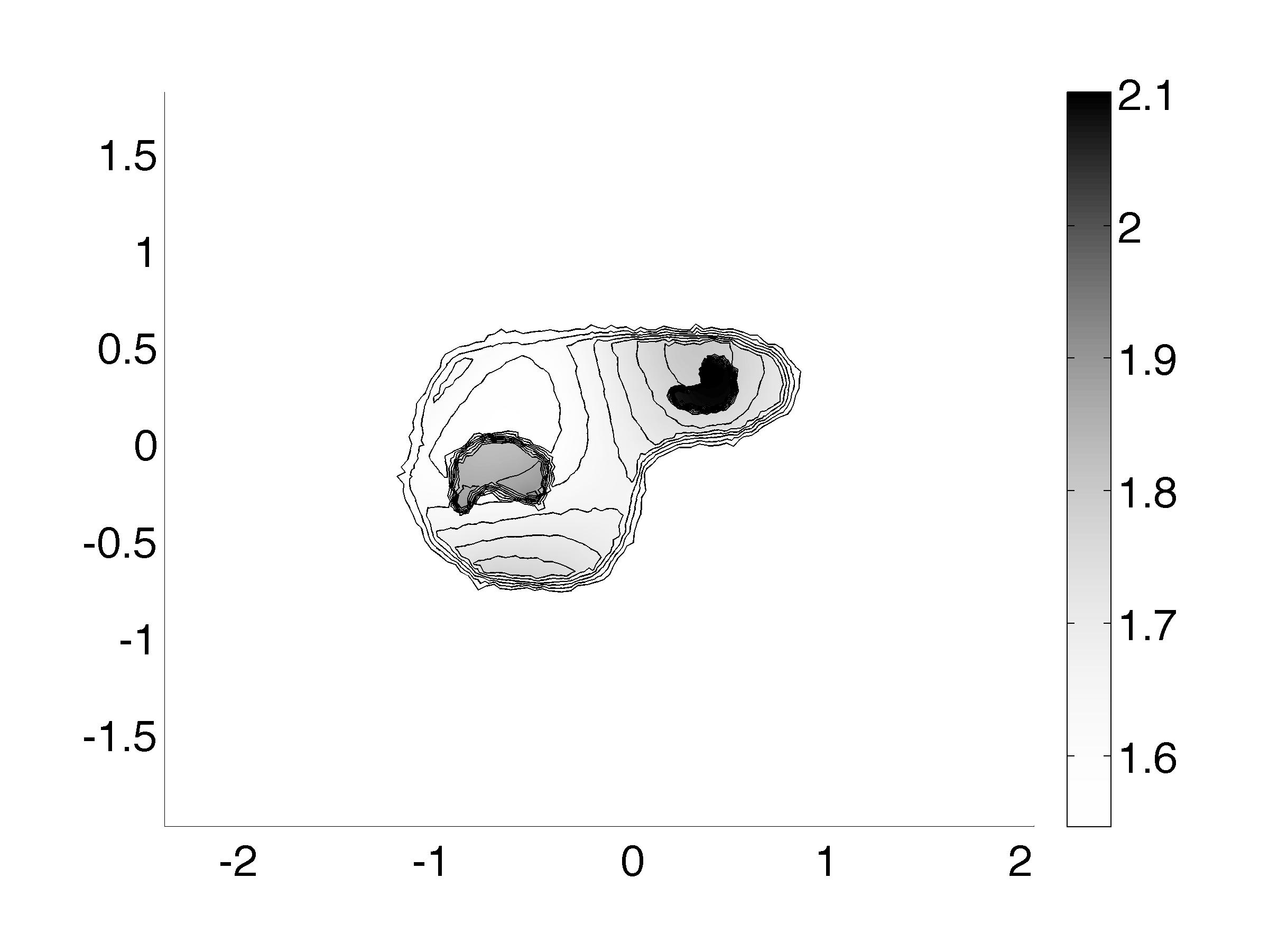
(c) Perturbed index’s real part

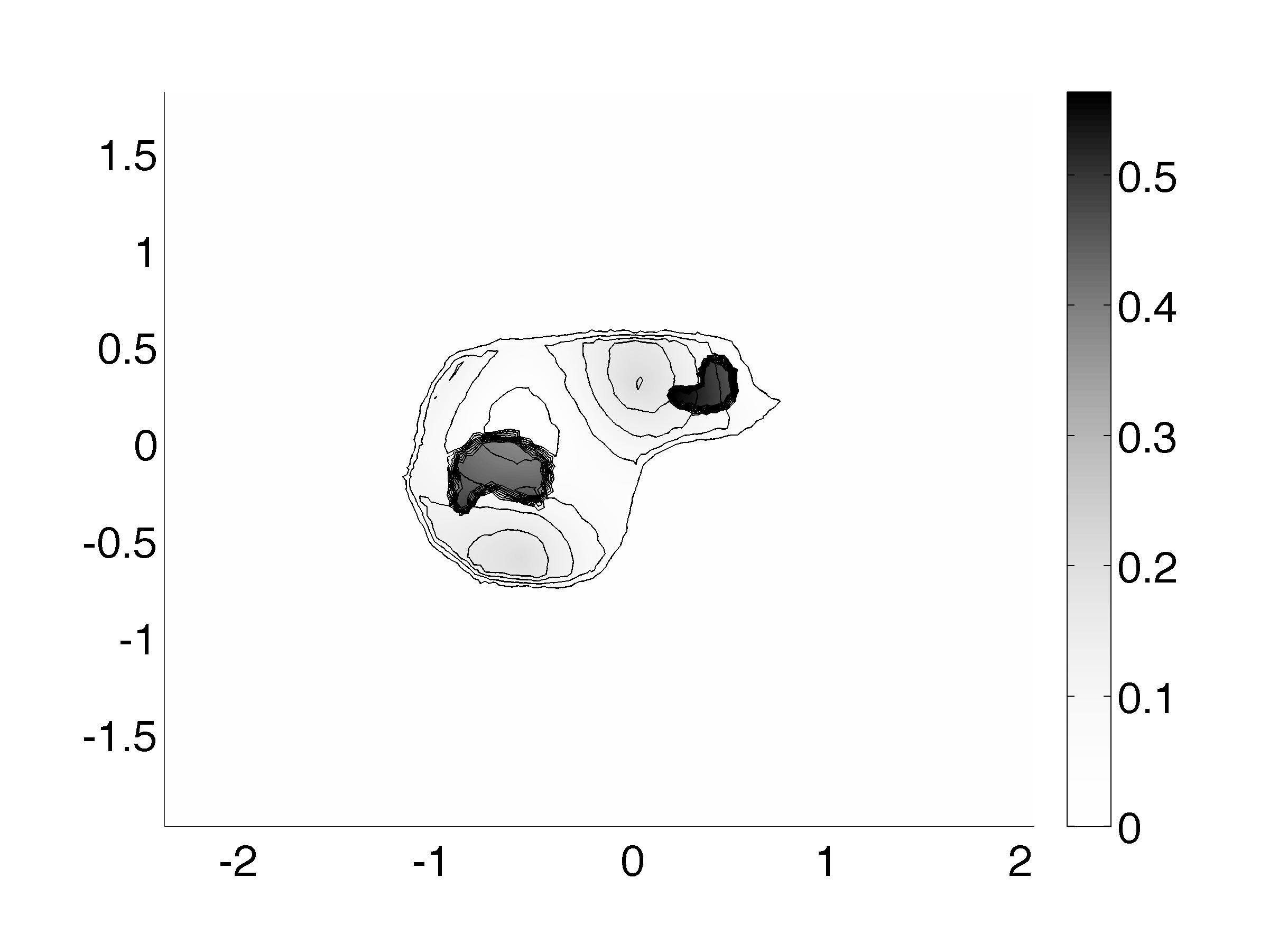
(d) Perturbed index’s imaginary part

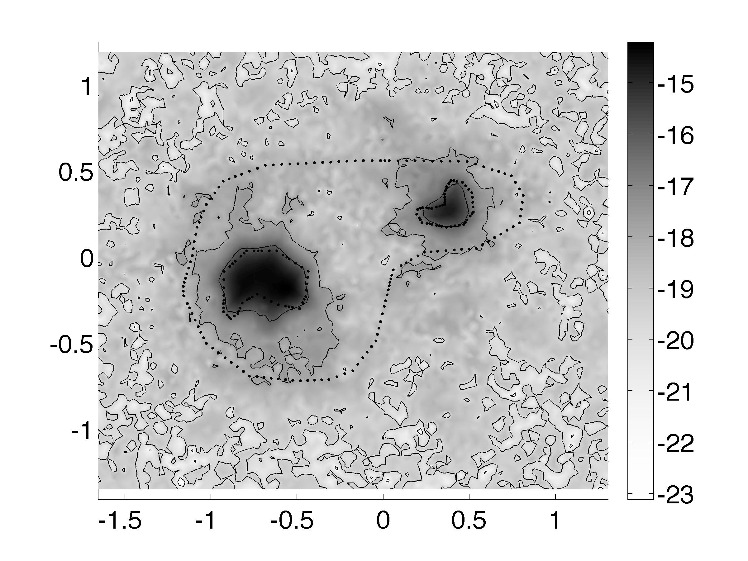
(e) Values of $\log_{10}\mathcal{M}_{W}(z)$ with $2\%$ noise

Number of iterations min med max Steepest descent 9 36 198 Gradient projection 9 28 400 Matlab’s fminunc 6 12 18 Matlab’s fmincon 8 13 21

(f)

Figure 7: Reconstruction of a non-trivial perturbation with the gradient projection algorithm

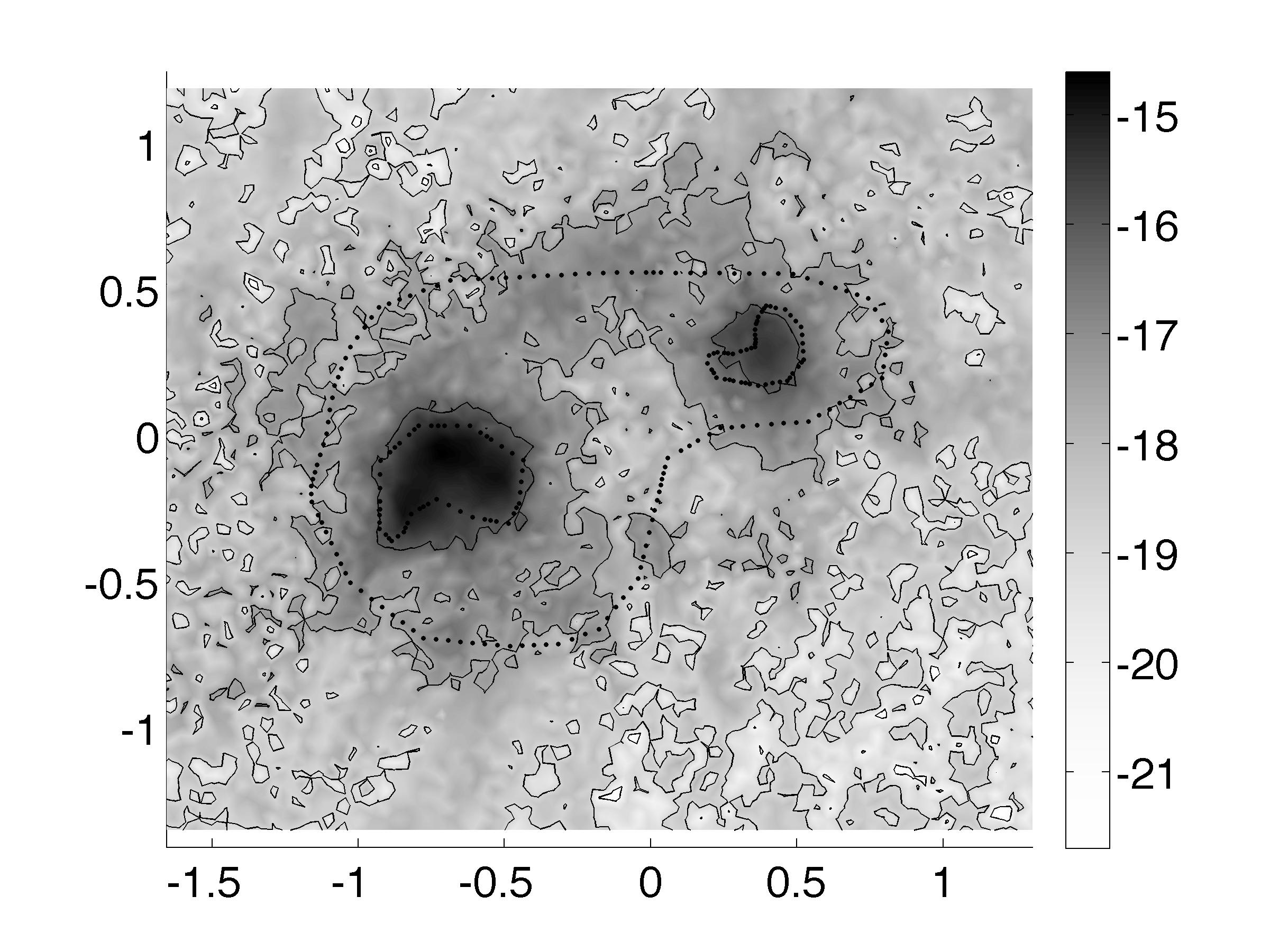
(a) Gradient projection algorithm

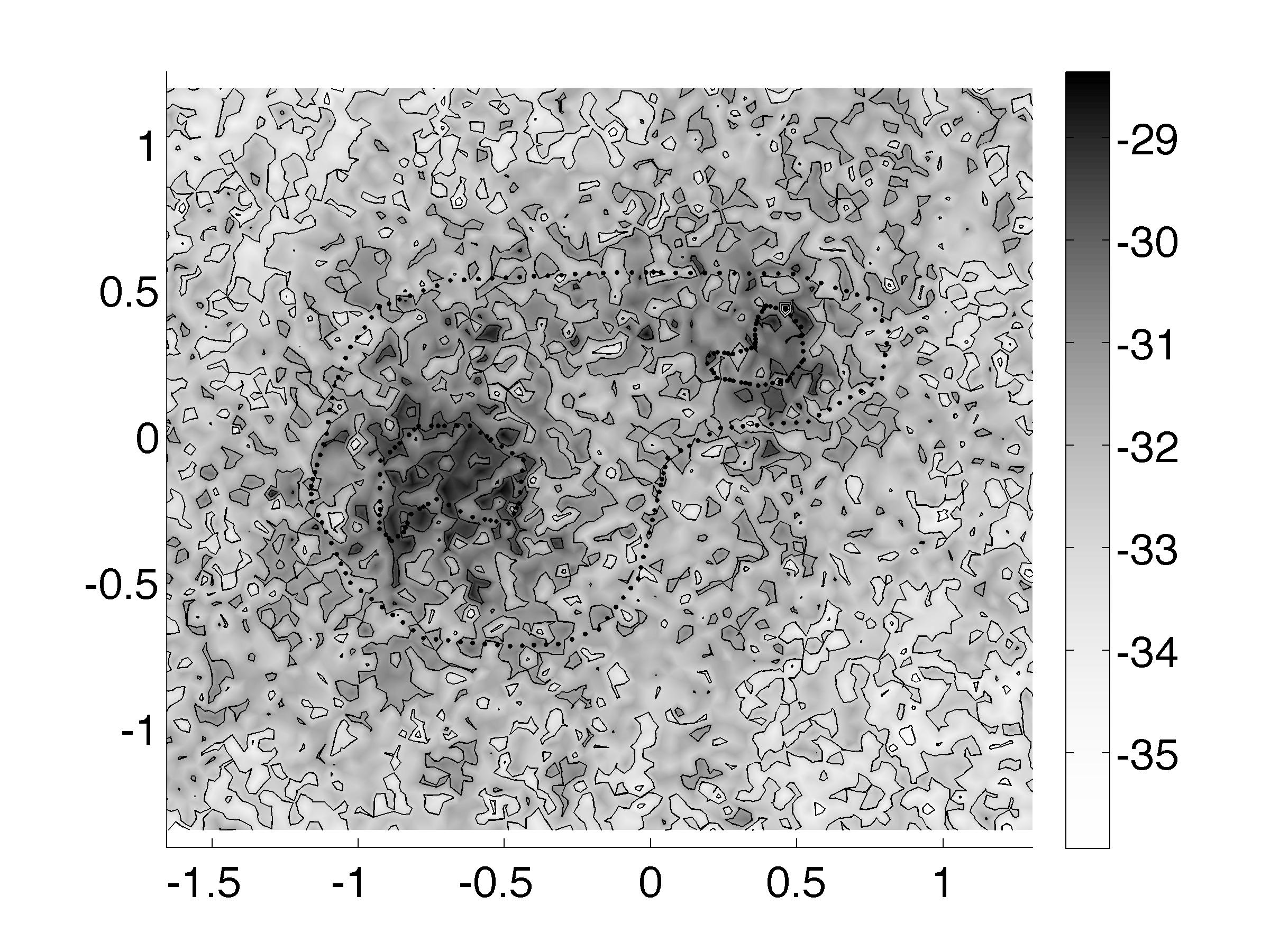
(b) Matlab’s fminunc function

Number of iterations	min	med	max
Steepest descent	7	41	216
Gradient projection	7	29	158
Matlab’s fminunc	7	11	17
Matlab’s fmincon	7	12	20

Figure 8: Reconstruction of a non-trivial perturbation with $2\%$ and limited far-field data

It is illustrated in figure 7e that comparable results are obtained on a more elaborate example with two non-convex and non-connected defects depicted in figures 7a–7d.

Besides, theorem 10 is stated under some physical restrictions arising from the use of the scattering operator $(\mathrm{id}+2ik\left\lvert\gamma\right\rvert^{2}F_{n_{0}})$. The numerical methods proposed in this section can however straightforwardly be extended to absorbing media and limited far-field data. We see in figure 7e that defects in complex valued indices are still correctly localized, even with $2\%$ uniform random noise added to the measurements.

Finally, even with limited far-field data, the gradient projection algorithm provided a satisfactory reconstruction, displayed in figure 8a. In this last example, the 99 evenly distributed incidence/measurement directions were taken in $[0,\,\frac{4}{3}\pi]$. Still, even with this fairly high amount of data, it is to be noted that the four algorithms presented in this paper do not yield comparable results in this case. Indeed, we see in figure 8b that Matlab’s functions fail to provide a usable reconstruction, despite our testing on a wide range of optimization parameters.

5 Conclusion

We have characterized the localization of defects in an inhomogeneous reference index by an optimization problem that is built only on the available data. Objective function and feasible set turn out to be very simple. This problem can thus be solved through a wide range of well known optimization methods, which we have numerically illustrated four examples of. Yet, some limitations were noticed, regarding the convergence speed on some cases and the required amount of data. Issues for which successful results were obtained using spectral methods in [8]. This opens the perspective of looking for some stabilization, or more robust versions of the proposed optimization algorithms.

Appendix

A.1 Derivatives of the objective function

We give here the derivatives of the functions involved in the computation of $\mathcal{M}_{W}(z)$ as defined by (16). However, since the values of the form $f_{W}$ are real, the differential can not be $\mathbb{C}$-linear. We therefore have to split the elements of $L^{2}(S^{d-1})$ into their real and imaginary parts and consider the objective function on pairs of real-valued functions to obtain proper $\mathbb{R}$-linear differentials. The induced gradient is then given in the following lemma.

Lemma 14.

The gradient of the form $\mathbf{f_{W}^{4}}:L^{2}(S^{d-1},\mathbb{R})\times L^{2}(S^{d-1},\mathbb{R})\to\mathbb{R}$, defined by

$$\mathbf{f_{W}^{4}}\begin{pmatrix}\phi\\ \psi\end{pmatrix}\mathrel{:}=\big{(}f_{W}(\Psi)\big{)}^{4},\quad\Psi\mathrel{:}=\phi+i\psi,$$

is given by

$$\nabla\mathbf{f_{W}^{4}}\begin{pmatrix}\phi\\ \psi\end{pmatrix}\mathrel{:}=4\begin{pmatrix}{\mathrm{Re}}\>Gf\begin{pmatrix}\phi\\ \psi\end{pmatrix}\\ {\mathrm{Im}}\>Gf\begin{pmatrix}\phi\\ \psi\end{pmatrix}\end{pmatrix},$$ (A-1)

where the function $Gf$ is an endomorphism on $(L^{2}(S^{d-1},\mathbb{R}))^{2}$ defined, with help of the self-adjoint parts $W_{R}\mathrel{:}=(W+W^{\star})/2$ and $W_{I}\mathrel{:}=(W-W^{\star})/2i$, by

$$G_{f}\begin{pmatrix}\phi\\ \psi\end{pmatrix}\mathrel{:}=\left\langle W_{R}\Psi,\,\Psi\right\rangle W_{R}\Psi+\left\langle W_{I}\Psi,\,\Psi\right\rangle W_{I}\Psi,\quad\Psi\mathrel{:}=\phi+i\psi.$$ (A-2)

Also, the second derivative of $\mathbf{f_{W}^{4}}$ is defined on $(L^{2}(S^{d-1},\mathbb{R}))^{4}$, for each point $(\phi,\psi)\in(L^{2}(S^{d-1},\mathbb{R}))^{2}$, by

$$\left[D^{2}\mathbf{f_{W}^{4}}\begin{pmatrix}\phi\\ \psi\end{pmatrix}\right](\begin{pmatrix}a\\ b\end{pmatrix},\begin{pmatrix}c\\ d\end{pmatrix})=4\left\langle\begin{pmatrix}{\mathrm{Re}}\>\left[H_{f}\begin{pmatrix}\phi\\ \psi\end{pmatrix}\right]\begin{pmatrix}a\\ b\end{pmatrix}\\ {\mathrm{Im}}\>\left[H_{f}\begin{pmatrix}\phi\\ \psi\end{pmatrix}\right]\begin{pmatrix}a\\ b\end{pmatrix}\end{pmatrix},\,\begin{pmatrix}c\\ d\end{pmatrix}\right\rangle,$$ (A-3)

where the operator $\left[H_{f}\begin{pmatrix}\phi\\ \psi\end{pmatrix}\right]$ is an endomorphism on $L^{2}(S^{d-1})$ defined for each $\begin{pmatrix}\phi\\ \psi\end{pmatrix}\in(L^{2}(S^{d-1}))^{2}$ by

$$\left[H_{f}\begin{pmatrix}\phi\\ \psi\end{pmatrix}\right]\begin{pmatrix}a\\ b\end{pmatrix}\mathrel{:}=2{\mathrm{Re}}\>\left\langle W_{R}\Psi,\,\Phi\right\rangle W_{R}\Psi+\left\langle W_{R}\Psi,\,\Psi\right\rangle W_{R}\Phi+2{\mathrm{Re}}\>\left\langle W_{I}\Psi,\,\Phi\right\rangle W_{I}\Psi+\left\langle W_{I}\Psi,\,\Psi\right\rangle W_{I}\Phi,$$

where $\Psi\mathrel{:}=\phi+i\psi$ and $\Phi\mathrel{:}=a+ib$.

Proof. First, for $\begin{pmatrix}\phi\\ \psi\end{pmatrix}$ and $\begin{pmatrix}u\\ v\end{pmatrix}$ in $L^{2}(S^{d-1},\mathbb{R})\times L^{2}(S^{d-1},\mathbb{R})$ we denote

$$\Psi\mathrel{:}=\phi+i\psi,$$

$$\Phi\mathrel{:}=u+iv.$$

Let then $\mathbf{f_{W}^{2}}:L^{2}(S^{d-1},\mathbb{R})\times L^{2}(S^{d-1},\mathbb{R})\to\mathbb{C}$ be defined by

$$\mathbf{f_{W}^{2}}\begin{pmatrix}\phi\\ \psi\end{pmatrix}\mathrel{:}=\left\langle W\Psi,\,\Psi\right\rangle_{L^{2}(S^{d-1})},$$

so we have $\mathbf{f_{W}^{4}}\begin{pmatrix}\phi\\ \psi\end{pmatrix}=\left\lvert\mathbf{f_{W}^{2}}\begin{pmatrix}\phi\\ \psi\end{pmatrix}\right\rvert^{2}$. Moreover, the operator $W$ is not self-adjoint but is nevertheless an endomorphism. Hence, we can use its real and imaginary parts as defined by

$$W_{R}\mathrel{:}=(W+W^{\star})/2,\quad W_{I}\mathrel{:}=(W-W^{\star})/2i.$$

It follows that $\left\langle W_{R}\Psi,\,\Psi\right\rangle={\mathrm{Re}}\>\left\langle W\Psi,\,\Psi\right\rangle$ and $\left\langle W_{I}\Psi,\,\Psi\right\rangle={\mathrm{Im}}\>\left\langle W\Psi,\,\Psi\right\rangle$. Since the operators $W_{R}$ et $W_{I}$ are self-adjoint, with $\Phi\mathrel{:}=u+iv$ we obtain

$$D\mathbf{f_{W}^{2}}\begin{pmatrix}\phi\\ \psi\end{pmatrix}\begin{pmatrix}u\\ v\end{pmatrix} =2{\mathrm{Re}}\>\left\langle W_{R}\Psi,\,\Phi\right\rangle+2i{\mathrm{Re}}\>\left\langle W_{I}\Psi,\,\Phi\right\rangle.$$

Hence, the differential of $\mathbf{f_{W}^{4}}$ is given by

$$D\mathbf{f_{W}^{4}}\begin{pmatrix}\phi\\ \psi\end{pmatrix}\begin{pmatrix}u\\ v\end{pmatrix} =2{\mathrm{Re}}\>\left\langle\left\langle W_{R}\Psi,\,\Psi\right\rangle+i\left\langle W_{I}\Psi,\,\Psi\right\rangle,\,2{\mathrm{Re}}\>\left\langle W_{R}\Psi,\,\Phi\right\rangle+2i{\mathrm{Re}}\>\left\langle W_{I}\Psi,\,\Phi\right\rangle\right\rangle$$

$$=4{\mathrm{Re}}\>\left\langle\left\langle W_{R}\Psi,\,\Psi\right\rangle W_{R}\Psi+\left\langle W_{I}\Psi,\,\Psi\right\rangle W_{I}\Psi,\,\Phi\right\rangle$$

$$=4{\mathrm{Re}}\>\left\langle Gf(\Psi),\,\Phi\right\rangle,$$

where $G_{f}$ is defined by (A-2). The gradient (A-1) is then written by recalling that for hermitian inner products, it holds that

$${\mathrm{Re}}\>\left\langle f,\,g\right\rangle=\left\langle\begin{pmatrix}{\mathrm{Re}}\>f\\ {\mathrm{Im}}\>f\end{pmatrix},\,\begin{pmatrix}{\mathrm{Re}}\>g\\ {\mathrm{Im}}\>g\end{pmatrix}\right\rangle.$$ (A-4)

Finally, we get the second derivative by differentiating the gradient. Since the operators $W_{R}$ and $W_{I}$ are $\mathbb{C}$-linear and self-adjoint, it comes

$$DG_{f}(\Psi)(\Phi)=2{\mathrm{Re}}\>\left\langle W_{R}\Psi,\,\Phi\right\rangle W_{R}\Psi+\left\langle W_{R}\Psi,\,\Psi\right\rangle W_{R}\Phi+2{\mathrm{Re}}\>\left\langle W_{I}\Psi,\,\Phi\right\rangle W_{I}\Psi+\left\langle W_{I}\Psi,\,\Psi\right\rangle W_{I}\Phi.$$

∎

As a consequence, we also have to adapt the projection $P_{\mathcal{C}_{z}}$ (17) and use its counterpart $\mathbf{P_{\mathcal{C}_{z}}}$ defined as an affine endomorphism of $L^{2}(S^{d-1},\mathbb{R})\times L^{2}(S^{d-1},\mathbb{R})$ by

$$\mathbf{P_{\mathcal{C}_{z}}}\begin{pmatrix}\phi\\ \psi\end{pmatrix}\mathrel{:}=\begin{pmatrix}{\mathrm{Re}}\>P_{\mathcal{C}_{z}}\Psi\\ {\mathrm{Im}}\>P_{\mathcal{C}_{z}}\Psi\end{pmatrix},\quad\Psi=\phi+i\psi.$$ (A-5)

The gradient of the objective function’s projection, denoted by $\mathbf{P_{f_{W}^{4}}}$, is then given by

$$\nabla\mathbf{P_{f_{W}^{4}}}\begin{pmatrix}\phi\\ \psi\end{pmatrix}=\begin{pmatrix}{\mathrm{Re}}\>{(\overset{\to}{P}_{\mathcal{C}_{z}})^{\star}}Gf({P_{\mathcal{C}_{z}}}\Psi)\\ {\mathrm{Im}}\>{(\overset{\to}{P}_{\mathcal{C}_{z}})^{\star}}Gf({P_{\mathcal{C}_{z}}}\Psi)\end{pmatrix},\quad\Psi=\phi+i\psi,$$

where ${\overset{\to}{P}_{\mathcal{C}_{z}}}$ is the linear part of the projection and where $G_{f}$ is given by (A-2).

A.2 Finite dimension approximation

For the finite dimension approximation, the operators ${W_{R}}$ and ${W_{I}}$ have a complex matrix representation. In order to write the gradient in more natural terms of matrix-vector products, we thus denote $\mathbf{W_{R}}$ and $\mathbf{W_{I}}$ the corresponding real valued expanded matrices defined by

$$\mathbf{W_{R}}\mathrel{:}=\begin{pmatrix}{\mathrm{Re}}\>({W_{R}})&-{\mathrm{Im}}\>({W_{R}})\\ {\mathrm{Im}}\>({W_{R}})&{\mathrm{Re}}\>({W_{R}})\end{pmatrix},\quad\mathbf{W_{I}}\mathrel{:}=\begin{pmatrix}{\mathrm{Re}}\>({W_{I}})&-{\mathrm{Im}}\>({W_{I}})\\ {\mathrm{Im}}\>({W_{I}})&{\mathrm{Re}}\>({W_{I}})\end{pmatrix}.$$

Moreover, we assume the standard change of basis $M^{\frac{1}{2}}$, where $M$ is a discretization of the inner product, so that the transposition correctly represents the adjoint of operators. Furthermore, with $\phi$ and $\psi$ two elements of the discretized version of $L^{2}(S^{d-1})$, in the basis $M^{\frac{1}{2}}$, denote

$$\mathbf{x}=\begin{pmatrix}\phi\\ \psi\end{pmatrix}.$$

With these notations it comes that

$$\mathbf{W_{R}}\mathbf{x}=\begin{pmatrix}{\mathrm{Re}}\>W_{R}(\phi+i\psi)\\ {\mathrm{Im}}\>W_{R}(\phi+i\psi)\end{pmatrix},\quad\mathbf{W_{I}}\mathbf{x}=\begin{pmatrix}{\mathrm{Re}}\>W_{I}(\phi+i\psi)\\ {\mathrm{Im}}\>W_{I}(\phi+i\psi)\end{pmatrix},$$

and by recalling (A-4), we have

$$\begin{array}[]{lll}\mathbf{x}^{T}\mathbf{W_{R}}\mathbf{x}&={\mathrm{Re}}\>\left\langle{W_{R}}(\phi+i\psi),\,(\phi+i\psi)\right\rangle&=\left\langle{W_{R}}(\phi+i\psi),\,(\phi+i\psi)\right\rangle,\\ \mathbf{x}^{T}\mathbf{W_{I}}\mathbf{x}&={\mathrm{Re}}\>\left\langle{W_{I}}(\phi+i\psi),\,(\phi+i\psi)\right\rangle&=\left\langle{W_{I}}(\phi+i\psi),\,(\phi+i\psi)\right\rangle.\end{array}$$

It follows from (A-1) that the (expanded) gradient of the form $f^{4}_{W}$ is given by

$$\nabla\mathbf{f_{W}^{4}}(\mathbf{x})=4\mathbf{W_{R}}\mathbf{x}(\mathbf{x}^{T}\mathbf{W_{R}}\mathbf{x})+4\mathbf{W_{I}}\mathbf{x}(\mathbf{x}^{T}\mathbf{W_{I}}\mathbf{x}).$$

It also follows from (A-3) that the corresponding hessian matrix $\mathbf{H}_{f^{4}_{W}}(\mathbf{x})$ is given by

$$\mathbf{H}_{f^{4}_{W}}(\mathbf{x})=8\mathbf{W_{R}}\mathbf{x}\otimes\mathbf{W_{R}}\mathbf{x}+4\mathbf{W_{R}}(\mathbf{x}^{T}\mathbf{W_{R}}\mathbf{x})+8\mathbf{W_{I}}\mathbf{x}\otimes\mathbf{W_{I}}\mathbf{x}+4\mathbf{W_{I}}(\mathbf{x}^{T}\mathbf{W_{I}}\mathbf{x}),$$

where the tensor product between two column vectors $\mathbf{a}\mathrel{:}=\begin{pmatrix}a_{1}\\ a_{2}\\ \vdots\end{pmatrix}$ and $\mathbf{b}\mathrel{:}=\begin{pmatrix}b_{1}\\ b_{2}\\ \vdots\end{pmatrix}$ is defined by the matrix given in columns by

$$\mathbf{a}\otimes\mathbf{b}\mathrel{:}=\begin{pmatrix}\mathbf{a}b_{1}&\mathbf{a}b_{2}\dots\end{pmatrix}.$$

Finally, it then comes from a straightforward calculation that the finite dimension approximations of the gradient and the hessian matrix for the form $\mathbf{P_{f_{W}^{4}}}$ are

$$\nabla\mathbf{P_{f_{W}^{4}}}(\mathbf{x})=\mathbf{\overset{\to}{P}}^{T}\nabla\mathbf{f_{W}^{4}}(\mathbf{P}_{\mathcal{C}_{z}}\mathbf{x}),$$

and

$$\mathbf{H}_{P_{f^{4}_{W}}}(\mathbf{x})=\mathbf{\overset{\to}{P}}^{T}\mathbf{H}_{f^{4}_{W}}(\mathbf{P}_{\mathcal{C}_{z}}\mathbf{x})\mathbf{\overset{\to}{P}},$$

where $\mathbf{\overset{\to}{P}}$ is the expanded matrix representation of the projection’s linear part.

References

- [1] T. Arens. Why linear sampling works. Inverse Problems, 20:163, 2004.
- [2] Thomas F. Coleman and Yuying Li. An interior trust region approach for nonlinear minimization subject to bounds. SIAM J. Optim., 6(2):418–445, 1996.
- [3] F. Collino, M’B. Fares, and H. Haddar. On the validation of the linear sampling method in electromagnetic inverse scattering problems. Research Report 4665, INRIA, 2002.
- [4] D. Colton. Inverse acoustic and electromagnetic scattering theory. In Gunther Uhlman, editor, Inside out: inverse problems and applications, volume 47 of Math. Sci. Res. Inst. Publ., pages 67–110. Cambridge Univ. Press, Cambridge, 2003.
- [5] D. Colton and A. Kirsch. A simple method for solving inverse scattering problems in the resonance region. Inverse Problems, 12(4):383–393, 1996.
- [6] D. Colton and R. Kress. Inverse acoustic and electromagnetic scattering theory, volume 93 of Applied Mathematical Sciences. Springer-Verlag, Berlin, second edition, 1998.
- [7] D. Colton, M. Piana, and R. Potthast. A simple method using Morozov’s discrepancy principle for solving inverse scattering problems. Inverse Problems, 13(6):1477–1493, 1997.
- [8] Y. Grisel, V. Mouysset, P-A. Mazet, and J-P. Raymond. Determining the shape of defects in non-absorbing inhomogeneous media from far-field measurements. Inverse Problems, 28:055003, 2012.
- [9] A. Kirsch. Characterization of the shape of a scattering obstacle using the spectral data of the far field operator. Inverse Problems, 14(6):1489–1512, 1998.
- [10] A. Kirsch. Factorization of the far-field operator for the inhomogeneous medium case and an application in inverse scattering theory. Inverse Problems, 15:413–429, 1999.
- [11] A. Kirsch. New characterizations of solutions in inverse scattering theory. Applicable Analysis, 76:319–350, 2000.
- [12] A. Kirsch. The MUSIC algorithm and the factorization method in inverse scattering theory for inhomogeneous media. Inverse Problems, 18(4):1025–1040, 2002.
- [13] A. Kirsch and N.I. Grinberg. The factorization method for inverse problems, volume 36 of Oxford Lecture Series in Mathematics and its Applications. Oxford University Press, Oxford, 2008.
- [14] A. I. Nachman, L. Päivärinta, and A. Teirilä. On imaging obstacles inside inhomogeneous media. J. Funct. Anal., 252(2):490–516, 2007.
- [15] R. Potthast. A survey on sampling and probe methods for inverse problems. Inverse Problems, 22(2):R1–R47, 2006.
- [16] J.B. Rosen. The gradient projection method for nonlinear programming. part i. linear constraints. Journal of the Society for Industrial and Applied Mathematics, 8(1):181–217, 1960.
- [17] G. Venkov. Atkinson-Wilcox expansion theorem for inhomogeneous media. In Math. Proc. R. Ir. Acad., volume 108, pages 19–25, 2008.