Self-trapping of Fermi and Bose gases under spatially modulated repulsive nonlinearity and transverse confinement

Abstract

We show that self-localized ground states can be created in the spin-balanced gas of fermions with repulsion between the spin components, whose strength grows from the center to periphery, in combination with the harmonic-oscillator (HO) trapping potential acting in one or two transverse directions. We also consider the ground state in the non-interacting Fermi gas under the action of the spatially growing tightness of the one- or two-dimensional (1D or 2D) HO confinement. These settings are considered in the framework of the Thomas-Fermi-von Weizsäcker (TF-vW) density functional. It is found that the vW correction to the simple TF approximation (the gradient term) is nearly negligible in all situations. The properties of the ground state under the action of the 2D and 1D HO confinement with the tightness growing in the transverse directions is investigated too for the Bose-Einstein condensate (BEC) with the self-repulsive nonlinearity.

I Introduction

One of fundamental conclusions produced by ongoing studies of the dynamics of matter waves in Bose-Einstein condensates (BECs) is that the effective local nonlinearity, induced by inter-atomic collisions, gives rise to robust bright solitons and soliton complexes chap01:njp2003b ; kono ; fatk ; Torner ; Morsch ; extra-reviews ; boris . In addition to their fundamental significance, the solitons may be employed in applications. In particular, the use of solitons in matter-wave interferometers should help to dramatically increase the accuracy of these devices, see Refs. Rosanov -Lev and a recent review billam2 .

In the usual settings, the existence of bright solitons requires the presence of the self-focusing nonlinearity. They may also be supported by nonlinear lattices, which feature alternation of spatial domains of self-focusing and defocusing, which give rise to the corresponding periodic pseudo-potential boris ; sala-nl . On the other hand, self-defocusing nonlinearities, acting in the combination with periodic linear (lattice) potentials, support bright solitons of the bandgap type kono ; fatk ; Morsch . Nevertheless, a common belief was that the self-defocusing per se could not give rise to bright solitons. The situation had changed when it was demonstrated that the repulsive cubic nonlinearity with the local strength growing with the distance from the center, $r$, faster than $r^{D}$, where $D$ is the spatial dimension, can readily support stable solitons and solitary vortices Barcelona ; Barcelona2 . In the same works, it was proposed how the corresponding profiles of the nonlinearity modulation can be created in BEC and nonlinear optics. In particular, the spatial modulation of the scattering length of inter-atomic collisions, induced by spatially inhomogeneous magnetic or optical fields via the Feshbach-resonance mechanism, can give rise to the required profile in BEC. Similarly, robust solitons and vortices were predicted in a more exotic model, with the constant strength of the defocusing nonlinearity but the diffraction coefficient decaying faster than $r^{-D}$ Zhong .

It may be interesting to implement this new option for the creation of bright solitons by purely repulsive nonlinearity landscapes in other physical settings. For instance, it was recently demonstrated that the same mechanism works too in one- and two-dimensional (1D and 2D) media with the repulsive quintic nonlinearity Zeng .

The present work aims to propose a way of creating bright solitons in Fermi gases, with balanced spin-up and spin-down components. The possibility is to combine the spatial growth of the s-wave scattering length, which accounts for the repulsion between the components, in one or two directions, and the harmonic-oscillator (HO) confining potential acting in the other directions. It should be noted that the dilute two-spin-component fermionic gases with the repulsive s-wave interaction do not feature phase coherence, as they are not superfluids lipparini . Nevertheless, their ground states can be accurately described by means of the density-functional theory hkt ; tosi ; Brandon .

Here we adopt the Thomas-Fermi-von Weizsäcker (TF-vW) form of the density functional to predict density profiles and chemical potentials of the Fermi droplets (i.e., bright solitons) in two different configurations, which are considered in Sections II and III, respectively: the quadratic growth of the scattering length in one direction ($z$) and transverse HO confinement in the $\left(x,y\right)$ plane; or the quadratic growth of the scattering length in the $\left(x,y\right)$ plane and HO confinement acting along $z$. Then, in Sections IV and V, following previous results obtained in the framework of the mean-field description of BEC sala-mod ; we ; Canary , we consider Fermi gases without intrinsic interactions (in particular, it may be a spin-polarized, i.e., single-spin-component, gas) and demonstrate that they give rise to localized ground states under the action of the 2D or 1D HO confinement, if its tightness, i.e., the corresponding confinement frequency, grows in the transverse directions faster than $\sqrt{|z|}$ or $r^{4}$, respectively. In addition, we demonstrate that the same confinements with the spatially growing tightness support, in a similar way, localized ground states in BEC with the self-repulsive nonlinearity.

II 1D nonlinearity modulation with the 2D transverse confinement for the spin-balanced interacting Fermi gas

In the presence of an external trapping potential $U_{\mathrm{ext}}(x,y,z)$, the Hohenberg-Kohn theorem hkt ensures that the single-body local density $n(x,y,z)$ of the ground state of a quantum system composed of interacting identical particles can be obtained by minimizing the energy functional,

$$E[n]=F[n]+\int\int\int U_{\mathrm{ext}}(x,y,z)\ n(x,y,z)\ dxdydz,$$ (1)

where $F[n]$ is an internal-energy functional, which is independent of $U_{\mathrm{ext}}(x,y,z)$. For the dilute normal Fermi gas with two equally-populated spin states, the TF-vW internal energy at zero-temperature is written as lipparini

$$F[n] = \int\int\int{\ }\left[{\frac{3}{5}}{\frac{\hbar^{2}}{2m}}(3\pi^{2})^{2/3}n^{5/3}+\lambda{\frac{\hbar^{2}}{8m}}{\frac{(\nabla n)^{2}}{n}}\right.$$ (2)

$$\left.+{\frac{1}{4}}g(z)n^{2}\right]dx\,dy\,dz,$$

with the nonlinearity strength determined by the s-wave fermion-up–fermion-down scattering length, which (as we assume in this work) may be modulated along the axial direction, $a_{\uparrow\downarrow}(z)$:

$$g(z)=\left(4\pi\hbar^{2}{/m}\right)a_{\uparrow\downarrow}(z).$$ (3)

The first term in functional (2) is the TF kinetic energy of the Fermi gas at zero temperature, while the second term is the vW correction to the kinetic energy of the inhomogeneous gas (the surface term). For the coefficient in front of the vW term, the phenomenological value, $\lambda=1/3$, may be adopted for non-superfluid fermions tosi . The third term in (2) is the mean-field approximation of the s-wave interaction between fermions with opposite spins.

The HO confinement in the transverse plane is accounted for by the external potential,

$$U_{\mathrm{ext}}(x,y)={(1/2)}m\omega_{\bot}^{2}r^{2},$$ (4)

with $r=(x^{2}+y^{2})^{1/2}$ and confinement radius $a_{\bot}=\sqrt{\hbar/(m\omega_{\bot})}$. We suppose that the spatially modulated scattering length also features the quadratic coordinate dependence, with a characteristic scale $a_{0}>0$,

$$a_{\uparrow\downarrow}(z)=\left(a_{0}/a_{\bot}^{2}\right)\ z^{2}.$$ (5)

By minimizing the energy functional (2), which is subject to the normalization constraint, imposed by the fixed total number of fermions,

$$N=\int\int\int n(x,y,z)\ dxdydz,$$ (6)

one derives the equation for the local density,

$$\left[-{\lambda}\nabla^{2}+(3\pi^{2})^{2/3}n^{2/3}+r^{2}+{\gamma}z^{2}n\right]\sqrt{n}=2\mu\sqrt{n},$$ (7)

with chemical potential $\mu$ fixed by normalization (6). Equation (7) is written in the scaled notation, with lengths measured in units of $a_{\bot}$ and energies in units of $\hbar\omega_{\bot}$. In this form, the equations depend on the single parameter, viz., the adimensional interaction strength,

$$\gamma\equiv 4\pi a_{0}/a_{\bot}.$$ (8)

Multiplying the left-hand side of Eq.(7) by $\sqrt{n}$ and integrating the result over the spatial coordinates, we obtain an expression for the chemical potential in terms of density $n(x,y,z)$:

$$\mu = {\frac{1}{2N}}\int\int\int\left[-{\lambda}\sqrt{n}\nabla^{2}\left(\sqrt{n}\right)+(3\pi^{2})^{2/3}\ n^{5/3}\right.$$ (10)

$$\left.+r^{2}n+{\gamma}z^{2}n^{2}\right]dx\,dy\,dz.$$

In the TF regime, when the vW correction is negligible, Eq. (7) for the density profile reduces to a cubic algebraic equation for $n^{1/3}$,

$$(3\pi^{2})^{2/3}n^{2/3}+r^{2}+{\gamma}z^{2}n=2\mu,$$ (11)

at $r<r_{\mathrm{TF}}$, and $n=0$ at $r>r_{\mathrm{TF}}$, where the TF radius is

$$r_{\mathrm{TF}}=\sqrt{2\mu}.$$ (12)

To find solutions of full equation (7), including the vW correction, an imaginary-time-derivative term was added to it, and ensuing stationary solutions were obtained by means of the finite-difference Crank-Nicolson predictor-corrector method, which keeps the fixed value of $N$ sala-numerics . In Fig. 1 we plot the so obtained 3D density profile $n(r,z)$ of the spin-balanced Fermi gas, produced by the numerical solution of Eq. (7) for $\mu=10$, the nonlinearity strength $\gamma=1$, and $\lambda=1/3$ (as said above), which corresponds to the self-trapped mode built of $N=612$ fermions. The figure shows that, while along the $r$ direction the density practically vanishes at $r_{\mathrm{TF}}=\sqrt{20}\simeq 4.47$, as predicted by the TF approximation, along the $z$ direction the density vanishes only at $|z|\rightarrow\infty$.

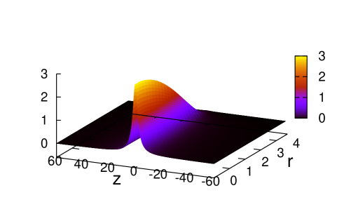
Figure 1: (Color online). The three-dimensional density profile $n(r,z)$ of the two-component spin-balanced Fermi gas, under the action of the 1D nonlinearity modulation, see Eq. (5), and the harmonic-oscillator confinement in the transverse plane [Eq. (4)]. The chemical potential is $\mu=10$, adimensional nonlinearity strength $\gamma=1$ [see Eq. (8)], and $\lambda=1/3$.

In Fig. 2 we plot the radial density, $n(r,z=0)$, for $N=100$ fermions, and compare the solutions of the full equation (7) with the TF approximation based on Eq.(11). The figure shows that the vW gradient term mainly affects the behavior of the density near the surface layer (see the insets in the figure): instead of vanishing at a finite distance $r_{\mathrm{TF}}$ from the center, the density vanishes at $r\rightarrow\infty$. Nevertheless, this effect is weak, and it becomes negligible for larger $N$.

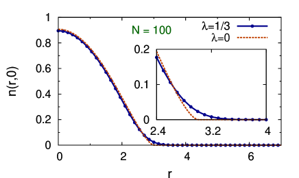
Figure 2: (Color online). Radial density $n(r,0)$ of the spin-balanced Fermi gas with nonlinearity strength $\gamma=1$ and number of particles $N=100$, in the same setting as in 1. Solid lines: solutions of the full equation (7), which includes the von Weizsäcker term with $\lambda=1/3$. Dashed lines: solutions produced by the Thomas-Fermi (TF) approximation based on Eq. (11) [i.e., Eq. (7) with $\lambda=0$]. Insets display a blowup of the structure of each state across the surface layer.

Similar features are exhibited by the dependence of the chemical potential, $\mu$, on the number of atoms, $N$, as shown in Fig. 3. The change of these dependences caused by the vW term is very small even for the state built of a dozen of atoms, see the inset in the figure. Thus, the simplified TF functional, disregarding the vW corrections ($\lambda=0$), is sufficient for the study of the ground state in the present model.

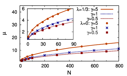
Figure 3: (Color online). Chemical potential $\mu$ (in units of $\hbar\omega_{\perp}$) vs. the number of particles, $N$, for the spin-balanced Fermi gas with nonlinearity strengths $\gamma=5,\ 1$ and $0.5$, in the same settings as in Figs. 1 and 2. Lines represent the dependences obtained from the full Thomas-Fermi-von Weizsäcker model, i.e., Eq. (7) with $\lambda=1/3$, while points correspond to the TF approximation ($\lambda=0$). The inset is a blowup of the dependence at small values of $N$.

Regarding the ground state, it is natural to expect that its width reduces with the growth of strength $\gamma$ of the self-repulsive nonlinearity. This expectation is confirmed by Fig. 4. In the upper and lower panels of this figure, we plot the radial and axial density profiles, viz., $n(r,z=0)$ and $n(r=0,z)$ respectively, for $N=100$, $\lambda=1/3$ (i.e., the vW is taken into account here, although it produces very little change) and three values of the nonlinearity strength, $\gamma=0.5$, $2$, and $5$.

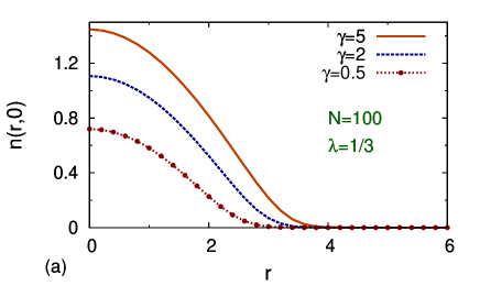
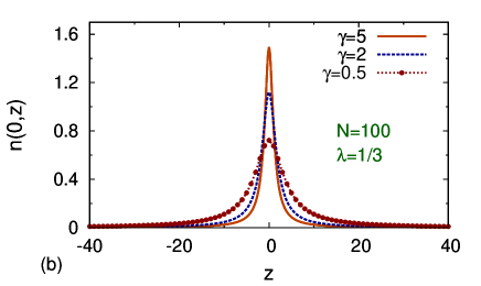
Figure 4: (Color online). (a) Radial $n(r,z=0)$ and (b) axial $n(r=0,z)$ density profiles of the ground state composed of $N=100$ fermions, for $\lambda=1/3$ in Eq. (7) and three values of nonlinearity strength $\gamma$, which is defined as per Eq. (8). The setting is the same as in Figs. 1-3.

As said above, chemical potential $\mu$ determines the total number $N$ of atoms in the ground state, hence its width increases with $\mu$, for fixed nonlinearity strength $\gamma$. In Fig. 5 we plot the root-mean-square (rms) radial size of the ground state, $\langle r^{2}\rangle^{1/2}$, versus $N$, for three values of the nonlinearity strengths, $\gamma=5,\ 1$ and $0.5$, using the the full equation (7) with $\lambda=1/3$ (lines in Fig. 5) and the TF approximation corresponding to $\lambda=0$ (points in Fig. 5). The results produced by the full and simplified models are essentially the same for different values of $\gamma$ and, virtually, for all $N$.

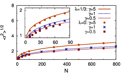
Figure 5: (Color online). The rms radial size $\langle r^{2}\rangle^{1/2}$ vs. the number of fermions, $N$, for nonlinearity strengths $\gamma=5,\ 1$ and $0.5$. Lines are produced by full equation (7) with $\lambda=1/3$, while points correspond to the TF approximation, $\lambda=0$. The inset shows the magnification of the dependence at small values of $N$. The setting is the same as in Figs. 1-4.

III 2D nonlinearity modulation with the 1D transverse confinement

We now consider the setting with the HO confinement acting along the longitudinal direction, viz.,

$$U_{\mathrm{ext}}(z)={(1/2)}m\omega_{z}^{2}z^{2},$$ (13)

cf. Eq. (4). On the other hand, the spatial modulation of the scattering length, $a_{\uparrow\downarrow}$, is adopted here to be two-dimensional, cf. Eq. (5):

$$a_{\uparrow\downarrow}(r)=\left(a_{0}/a_{z}^{2}\right)\ r^{2},$$ (14)

with $a_{0}>0$, where $a_{z}=\sqrt{\hbar/(m\omega_{z})}$ is the characteristic length of the longitudinal HO confinement (13). Thus, the present setting is a reverse of that considered in the previous section.

The corresponding TF-vW internal energy is

$$F[n] = \int\int\int{\ }\left[{\frac{3}{5}}{\frac{\hbar^{2}}{2m}}(3\pi^{2})^{2/3}n^{5/3}+\lambda{\frac{\hbar^{2}}{8m}}{\frac{(\nabla n)^{2}}{n}}\right.$$ (16)

$$+\left.{\frac{1}{4}}g(r)n^{2}\right]\ dx\,dy\,dz,$$

with $g(r)$ given by Eq. (3), in which $a_{\uparrow\downarrow}(z)$ is replaced by $a_{\uparrow\downarrow}(r)$, see Eq. (14). By minimizing the full energy functional, $E[n]=F[n]+\int\int\int U_{\mathrm{ext}}(z)n(x,y,z)dxdydz$, with the constraint of the normalization of $n(\mathbf{r})$, we obtain

$$\left[-{\lambda}\nabla^{2}+(3\pi^{2})^{2/3}n^{2/3}+z^{2}+{\Gamma}r^{2}n\right]\sqrt{n}=2\mu\sqrt{n},$$ (17)

cf. Eq. (7). In Eq. (17) lengths are measured in units of $a_{z}$, and energies in units of $\hbar\omega_{z}$, which leaves, as the single control parameter, the adimensional strength of the nonlinearity,

$$\Gamma\equiv 4\pi a_{1}/a_{z},$$ (18)

cf. Eq. (8).

In the TF approximation, which, as before, neglects the vW gradient term, the density profile, $n(r,z)$, satisfies an algebraic equation [cf. Eq. (11)]:

$$(3\pi^{2})^{2/3}n^{2/3}+z^{2}+{\Gamma}r^{2}n=2\mu.$$ (19)

Setting $n(r,z)=0$ in Eq.(19), one gets the TF axial size of the ground state, $z_{\mathrm{TF}}=\sqrt{2\mu}$, with $n=0$ at $|z|>z_{\mathrm{TF}}$ in the TF approximation, cf. Eq. (12).

In Fig. 6 the 3D density profile $n(r,z)$ of the Fermi gas is plotted for $\mu=10$, $\Gamma=2$, and $\lambda=1/3$ in Eq. (17). The figure shows that, while along the $z$ direction the density practically vanishes at $z_{\mathrm{TF}}=\sqrt{20}\simeq 4.47$, along $r$ the density vanishes only at $r\rightarrow\infty$.

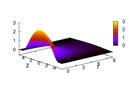
Figure 6: (Color online) Three-dimensional density profile $n(r,z)$ of the two-component spin-balanced Fermi gas under the 1D external confinement, see Eq. (13), and 2D modulation of the local nonlinearity in the transverse plane [Eq. (14)]. The chemical potential is $\mu=10$, adimensional nonlinearity strength is $\Gamma=2$, and $\lambda=1/3$ is adopted in Eq. (17). Lengths are measured in units of $a_{z}$, and energies in units of $\hbar\omega_{z}$.

In Fig. 7 we plot axial density $n(0,z)$ for two values of the chemical potential, $\mu=$ $10$ and $20$, in panels (a) and (b), respectively, both taken with $\Gamma=2$. In this figure we compare solutions of the full equation (17) to their counterparts produced by the TF approximation, which is based on Eq. (19). The figure shows, once again, that the vW gradient term mainly affects the behavior of the density in the surface layer: Instead of vanishing at a finite distance ($z_{\mathrm{TF}}$) from the center of the cloud, it vanishes at $|z|\rightarrow\infty$. However, this effect is weak, becoming negligible at larger values of the chemical potential.

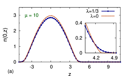
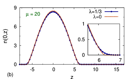
Figure 7: (Color online). Axial density profiles $n(0,z)$ of the two-component spin-balanced Fermi gas under the 1D confinement [Eq. (13)] and 2D modulation of the nonlinearity [Eq. (14)], whose global strength is $\Gamma=2$,[see Eq. (18), for two values of the chemical potential: $\mu=10$ (a) and $\mu=20$ (b). Solid lines: solutions of Eq. (17) with $\lambda=1/3$; dashed lines: solutions of Eq. (19), i.e., Eq. (17) with $\lambda=0$. Units are the same as in Fig. 6.

As shown in Fig. 8, a similar phenomenon is observed in the dependences of the chemical potential $\mu$ on $N$, which were produced by the full equation 17 with $\lambda=1/3$ (lines in Fig. 8), and by the TF approximation (19) (points in Fig. 8). The effect of the vW gradient term remains inconspicuous even at small values of $N$, and at all values of $\Gamma$.

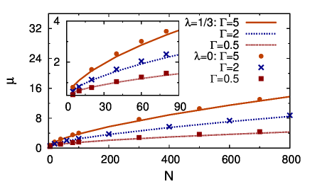
Figure 8: (Color online). Chemical potential $\mu$ versus number $N$ of fermionic atoms for the two-component spin-balanced Fermi gas under the 1D confinement and 2D modulation of the local nonlinearity. The nonlinearity strength takes values $\Gamma=5,\ 2$ and $0.5$. Lines are obtained from full equation (17), while points correspond to the TF approximation ($\lambda=0$). Energies are in units of $\hbar\omega_{z}$.

A natural expectation that the radial width of the ground state reduces with the increase of the nonlinearity strength, $\Gamma$ [i.e., the gas is stronger compressed by the effective nonlinear (pseudo)potential], is confirmed by Fig. 9. In this figure we plot the rms size of the ground state, $\langle z^{2}\rangle^{1/2}$, versus the number of particles, $N$, for three values of the nonlinearity strength, $\Gamma=5,\ 2$ and $0.5$, using the full equation (17) with $\lambda=1/3$, the TF approximation corresponding to $\lambda=0$ (lines and points, respectively, in Fig. 9). Thus, we conclude that the effect of the vW term is inessential in this setting too.

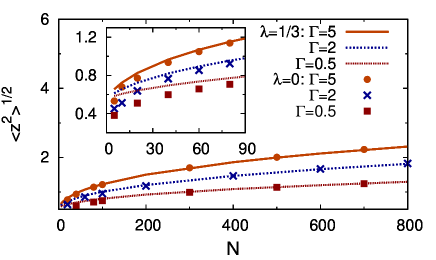
Figure 9: (Color online). The rms size $\langle z^{2}\rangle^{1/2}$ vs. number $N$ of fermions of the ground state with nonlinearity strengths $\Gamma=5,\ 2$ and $0.5$. Lines and points represent the results obtained, respectively, from the full equation (17) with $\lambda=1/3$, and from the TF approximation corresponding to $\lambda=0$. The inset shows details of the dependences at smaller values of $N$. The setting is the same as in Figs. 6-8.

IV Self-trapping in the non-interacting Fermi gas and self-repulsive BEC due to the axial modulation of the 2D confinement

IV.1 The non-interacting Fermi gas under the 2D confinement with the strength growing in the axial direction

In the spin-balanced ideal Fermi gas, without any interaction between the two spin components, or the single-component spin-polarized gas, in which direct interactions are suppressed by the Pauli principle, it is possible to induce self-trapping along the longitudinal direction ($z$) by introducing a $z$-dependent modulation of the transverse HO confinement frequency, $\omega_{\bot}$. The corresponding energy functional is

$$E[n] = \int\int\int\left[{\frac{3}{5}}{\frac{\hbar^{2}}{2m}}(3\pi^{2})^{2/3}n^{5/3}+\lambda{\frac{\hbar^{2}}{8m}}{\frac{(\nabla n)^{2}}{n}}\right.$$ (21)

$$\left.+{\frac{1}{2}}m\omega_{\bot}^{2}(z)(x^{2}+y^{2})\,n\right]\ dx\,dy\,dz\;.$$

By minimizing this functional, subject, as before, to the constraint of the normalization of $n(\mathbf{r})$, one obtains

$$\left[-{\lambda}\nabla^{2}+(3\pi^{2})^{2/3}n^{2/3}+\omega_{\bot}^{2}(z)r^{2}\right]\sqrt{n}=2\mu\sqrt{n},$$ (22)

where $\mu$ is the chemical potential fixed by the total number of atoms, $N$ [see Eq. (6)]. Solving Eq.(22), we aim to produce the longitudinal density profile,

$$n_{1}(z)\equiv\int\int n(\mathbf{r})\ dxdy.$$ (23)

The TF approximation corresponds, as above, to setting $\lambda=0$ in Eq. (22), which makes it a simple algebraic equation that immediately yields an explicit solution [this was not available in the presence of the interaction between the spin components, cf. Eqs. (7) and (11)]:

$$n\left(r,z\right)=\left\{\begin{array}[]{c}\left(3\pi^{2}\right)^{-1}\left[2\mu-\omega_{\perp}^{2}(z)r^{2}\right]^{3/2},~{}\mathrm{at}~{}~{}\omega_{\perp}^{2}(z)r^{2}<2\mu,\\ 0,~{}\mathrm{at}~{}~{}\omega_{\perp}^{2}(z)r^{2}>2\mu\end{array}\right.$$ (24)

(obviously, the solution exists only for $\mu>0$). This solution is physically meaningful if its norm converges, which implies the convergence of $\int_{0}^{z}r_{\mathrm{TF}}^{2}\left(z^{\prime}\right)dz^{\prime}\equiv 2\mu\int_{0}^{z}\omega_{\perp}^{-2}\left(z^{\prime}\right)dz^{\prime}$ at $z\rightarrow\infty$. The eventual condition is that $\omega_{\perp}^{2}(z)$ must grow faster than $|z|$, i.e.,

$$\omega_{\perp}(z)/\sqrt{|z|}\rightarrow\infty,$$ (25)

at $|z|\rightarrow\infty$. Further, the substitution of explicit solution (24) into Eq. (23) makes it possible to obtain the TF approximation for $n_{1}$ in an explicit form too:

$$n_{1}(z)={\frac{16\sqrt{2}}{15\pi}}\left({\frac{m\mu}{\hbar^{2}}}\right)^{5/2}a_{\bot}^{4}(z)\;.$$ (26)

Below we consider the most natural modulation form,

$$\omega_{\bot}(z)=\alpha z^{2}+\beta,$$ (27)

with positive $\alpha$ and $\beta$. Obviously, it satisfies condition (25). In Fig. 10 we plot longitudinal profiles of the reduced density (23) for the $z$-dependent modulation of the transverse-confinement strength given by Eq. (27) with $\alpha=0.01$ and $\beta=1$. Dots in Fig. 10 represent analytical result (26), and lines depict (for the sake of checking the correctness of the analytical result) the numerical solution of Eq. (22) with $\lambda=0$, obtained as in Ref. sala-numerics [in the latter case, the 3D density is numerically integrated in the transverse plane to reduce it to $n_{1}$, see Eq. (23).

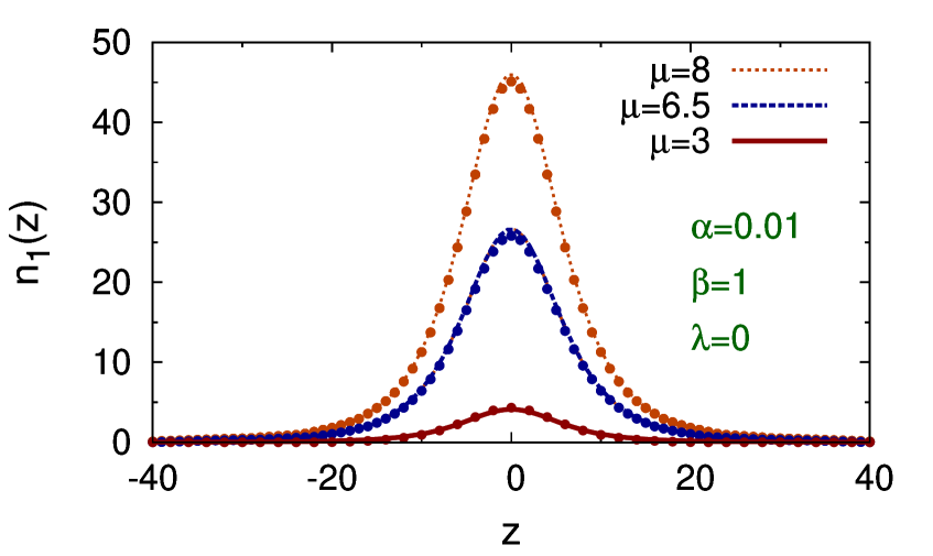
Figure 10: (Color online). Profiles of the longitudinal density $n_{1}(z)$ of the non-interacting Fermi gas, with the $z$-dependent modulation of the transverse-confinement frequency, chosen as per Eq. (27) with $\alpha=0.01$ and $\beta=1$, for three values of the chemical potential: $\mu=8,~{}6.5$, and $5$. Lines: a numerical solution of Eq. (22) for $\lambda=0$. Points: analytical result (26).

To address effects of the vW term in the present case, in Fig. 11 we plot chemical potential $\mu$ as a function of the number of atoms $N$, using the numerical solutions of Eq. (22) with $\lambda=1/3$ and $\lambda=0$. It is seen that the effect of the vW gradient term is again very weak, for any number of particles. For the same purpose, in Fig. 12 we plot the radial density, $n(r,z=0)$, as found from the full equation and produced by the TF approximation, for the same set of values of the chemical potential as in Fig. 10.

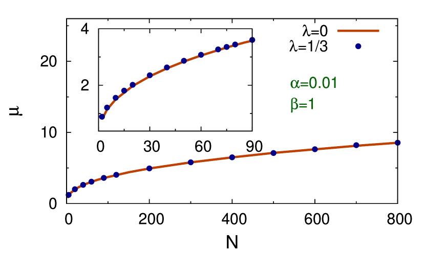
Figure 11: (Color online). Chemical potential $\mu$ vs. the number of fermionic atoms, $N$, of the ground state of the non-interacting Fermi gas subject to modulation (27) of the frequency of the transverse confinement. As indicated in the figures, the TF approximation ($\lambda=0$) produces the dependence which is very close to that generated by the full model, including the von Weizsäcker term ($\lambda=1/3$). The inset is a blowup of the dependence at small values of $N$.

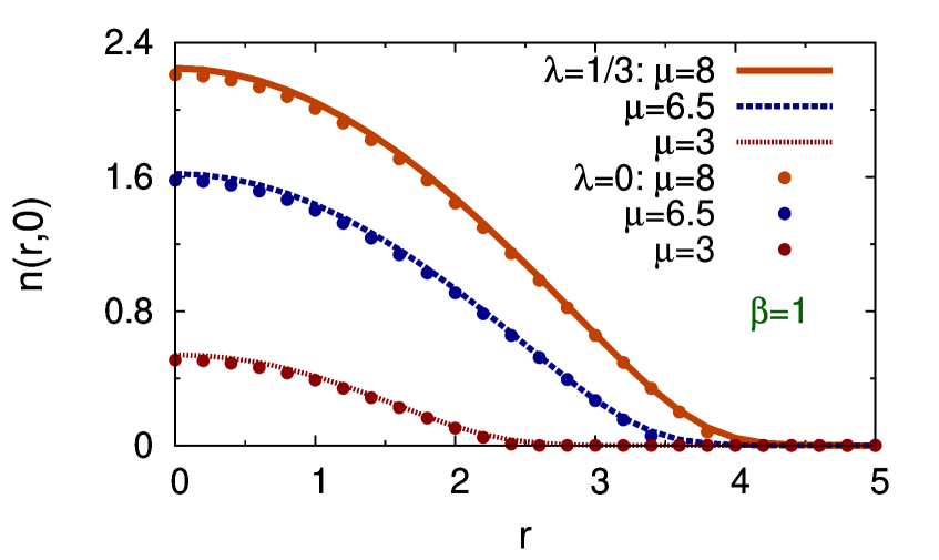
Figure 12: (Color online). Radial density $n(r,z=0)$ of the non-interacting Fermi gas, with the modulation of the frequency of the transverse confinement defined by Eq. (27), for three values of the chemical potential: $\mu=8,6.5$ and $3$. As above, symbols $\lambda=1/3$ and $\lambda=0$ designate, severally, the results produced by the full equation (22), and by the TF approximaiton (24). Units the same as in Fig. 10.

IV.2 A self-repulsive bosonic condensate under the 2D confinement with the strength growing in the axial direction

A mechanism of the formation of the localized ground state, similar to that presented in the previous section, may be applied to BEC with repulsive interactions between atoms, subject to the action of the 2D confinement in the plane of $\left(x,y\right)$, with the tightness growing along $z$. The respective effective 1D equation for the mean-field wave function, $\Phi\left(z,t\right)$, was derived in Ref. Canary , starting from the 3D Gross-Pitaevskii equation:

$$i\hbar\frac{\partial\Phi}{\partial t}=-\frac{\hbar^{2}}{2m}\frac{\partial^{2}\Phi}{\partial z^{2}}+\hbar\omega_{\perp}(z)\sqrt{1+4a_{s}|\Phi|^{2}}\Phi,$$ (28)

where $\omega_{\perp}$ is the same trapping frequency as above [cf. Eq. (22)], $m$ the atomic mass, $a_{s}>0$ the scattering length of the inter-atomic interactions, and the total number of bosons is given by

$$N=\int_{-\infty}^{+\infty}\left|\Phi(z)\right|^{2}dz$$ (29)

(in Ref. Canary , the norm of the 1D wave function was $1$, while $a_{s}$ in Eq. (28) was replaced by $Na_{s}$). Looking for a stationary state as $\Phi\left(z,t\right)=a_{s}^{-1/2}\exp\left(-i\mu T\right)U(Z)$, where $T\equiv\left(\hbar/ma_{s}^{2}\right)t$ and $Z\equiv z/a_{s}$, we arrive at an equation for real function $U(Z)$:

$$\mu U=-\frac{1}{2}\frac{d^{2}U}{dZ^{2}}+\Omega_{\perp}(Z)\sqrt{1+4U^{2}}U,$$ (30)

with $\Omega_{\perp}\equiv\left(ma_{s}^{2}/\hbar\right)\omega_{\perp}$. The TF approximation for solutions of Eq. (30) is obvious:

$$U(Z)=\left\{\begin{array}[]{c}\left(2\Omega_{\perp}(Z)\right)^{-1}\sqrt{\mu^{2}-\Omega_{\perp}^{2}(Z)},~{}\mathrm{at}~{}\Omega_{\perp}(Z)<\mu,{}\\ 0,~{}\mathrm{at}~{}\Omega_{\perp}(Z)\geq\mu\text{,}\end{array}\right.$$ (31)

cf. Eq. (24).

If, in particular, $\omega_{\perp}(z)$ grows faster than $\sqrt{|z|}$ at $|z|\rightarrow\infty$ [i.e., it obeys condition (25)], the TF approximation gives rise to a simple asymptotic dependence of the total number of bosonic atoms on the chemical potential: as follows from the substitution of expression (31) into Eq. (29),

$$N(\mu)=\int_{-\infty}^{+\infty}U^{2}(Z)dZ\approx\frac{\mu^{2}}{4}\int_{-\infty}^{+\infty}\frac{dZ}{\Omega_{\perp}^{2}(Z)}$$ (32)

for $\mu$ large enough. On the other hand, if $\omega_{\perp}$ grows slower at $|z|\rightarrow\infty$, namely, $\Omega_{\perp}(Z)\approx\Omega_{0}|Z|^{\alpha}$, with $\alpha\leq 1/2$, Eqs. (31) and (29) yield, in the limit of $\mu\rightarrow\infty$:

$$N(\mu)\approx\left\{\begin{array}[]{c}\left(\mu/\Omega_{0}\right)^{2}\ln\left(\mu/\mu_{0}\right),~{}\mathrm{for}~{}\alpha=1/2,\\ \alpha\left(1-2\alpha\right)^{-1}\left(\mu/\Omega_{0}\right)^{1/\alpha},~{}\mathrm{fort}~{}\alpha<1/2,\end{array}\right.$$ (33)

where constant $\mu_{0}$ is determined by the structure of $\Omega_{\perp}(Z)$ at finite values of $Z$. Note that both results (32) and (33) satisfy the “anti-Vakhitov-Kolokolov” (anti-VK) criterion, $dN/d\mu>0$, which implies the dynamical stability of the trapped modes in the case of the self-repulsive nonlinearity HS .

V Self-trapping in the self-repulsive BEC and non-interacting Fermi gas due to the radial modulation of the 1D confinement

The mechanism of the formation of the localized ground state in the non-interacting Fermi gas subject to the action of the HO trapping potential, whose strength grows from the center, can also be applied to the case when the potential acts only in one direction, $z$, while its tightness, $\omega_{z}^{2}$, is made a growing function of the transverse radial coordinate, $r$. Similar to the situation considered in the previous section, this mechanism applies not only to fermions, but also to the self-repulsive BEC under the same type of the confinement.

In terms of such a BEC setting, a system of equations for the 2D mean-field wave function, $\Phi\left(x,y,t\right)$, and the effective thickness of the condensate, $\eta(x,y)$, was derived in Ref. we :

$$i{\frac{\partial\Phi}{\partial t}} = \left[-{\frac{1}{2}}\nabla_{\bot}^{2}+\gamma(r)\eta^{-1}\Phi+(1/4)\left(\eta^{-2}+\eta^{2}\right)\right]\Phi,$$ (34)

$$\eta^{4} = 1+\gamma(r)\left|\Phi\right|^{2}\eta,$$ (35)

$$\gamma(r) \equiv 2a_{s}\sqrt{2\pi m\omega_{z}(r)/\hbar},$$ (36)

where $a_{s}>0$ is the scattering length of the repulsive interactions between bosonic atoms, and $\nabla_{\bot}^{2}$ is the Laplacian acting in the plane of $\left(x,y\right)$. A straightforward analysis demonstrates that Eqs. (34) and (35) can be reduced to a single 2D nonpolynomial Schrödinger equation,

$$i{\frac{\partial\Phi}{\partial t}} = \left[-{\frac{1}{2}}\nabla_{\bot}^{2}+\Gamma(r)|\Phi|^{4/3}\right]\Phi,$$ (37)

$$\Gamma(r) \equiv \frac{{5}}{4}\left(\gamma(r)\right)^{2/3},$$ (38)

provided that the local density of the condensate is large enough:

$$\gamma\left|\Phi\right|^{2}\gg 1.$$ (39)

Stationary solutions to Eq. (37) with chemical potential $\mu$ are looked for as

$$\Phi\left(x,y,t\right)=e^{-i\mu t}U\left(r\right),$$ (40)

with real function $U(r)$ obeying the radial equation,

$$\mu U=-\frac{1}{2}\left(\frac{d^{2}U}{dr^{2}}+\frac{1}{r}\frac{dU}{dr}\right)+\Gamma(r)U^{7/3},$$ (41)

the respective number of atoms being

$$N=2\pi\int_{0}^{\infty}\left(U(r)\right)^{2}rdr.$$ (42)

Under the same conditions, a similar equation for a functional-density wave function $U$ can be derived for the non-interacting Fermi gas by the reduction of the 3D density-functional description to 2D, as shown in Ref. David :

$$\mu U={-\nabla_{\bot}^{2}U+C_{\mathrm{2D}}}\left({\omega_{z}(r)}\right)^{1/3}{{{{U}^{7/3}}}},$$ (43)

where $C_{\mathrm{2D}}\equiv\sqrt{{3/5}}{(6/(2s+1))^{2/3}}\pi$, and $s$ is the semi-integer spin of the fermions. Note that, in the bosonic and fermionic settings alike, Eqs. (37), (38) and (43) demonstrate that the coefficient in front of the nonlinear term with total power $7/3$ is proportional to $\left({\omega_{z}(r)}\right)^{1/3}$.

The ground state can be constructed, as above, by means of the TF approximation, which neglects the derivatives in Eq. (41):

$$U_{\mathrm{TF}}(r)=\left[\mu/\Gamma(r)\right]^{3/4},$$ (44)

hence the corresponding dependence between the chemical potential and norm (42) takes a simple form,

$$N_{\mathrm{TF}}=G\mu^{3/2},~{}G\equiv 2\pi\int_{0}^{\infty}\frac{rdr}{\left[\Gamma(r)\right]^{3/2}},$$ (45)

cf. Eqs. (32) and (33). Note that the TF approximation (44) yields a fully continuous wave function (similar to that obtained by means of the TF approximation in Ref. Barcelona , in the model with the spatially growing strength of the cubic self-defocusing nonlinearity in the nonlinear Schrödinger equation), unlike the ones found above in the form of Eqs. (24) and (31), which imply divergence of the derivatives at the boundary between the nonzero and zero parts of the solution, $\omega_{\perp}(z)r=\sqrt{2\mu}$and $\Omega_{\perp}(Z)=\mu$, respectively.

According to Eq. (45), the norm of the trapped mode converges if $\Gamma(r)$ grows at $r\rightarrow\infty$ faster than $r^{4/3}$, i.e., as it follows from Eqs. (38) and (36), the transverse-trapping frequency, $\omega_{z}(r)$, must grow faster than $r^{4}$, i.e.,

$$\omega_{z}(r)/r^{4}\rightarrow\infty$$ (46)

at $r\rightarrow\infty$. Note that the similar condition obtained in the setting considered in the previous section was much weaker, requiring only that $\omega_{\perp}(z)$ had to grow faster than $\sqrt{|z|}$at $|z|\rightarrow\infty$, see Eq. (25). It is also worthy to note that the trapped TF modes exist with $\mu>0$, as well as solutions (24) and (31) considered in the previous section.

In the present notation, the condition (39) of the applicability of Eq. (37) for the bosonic gas takes the simple form, if TF approximation (44) is used:

$$\mu^{3/2}\gg 1.$$ (47)

This condition guarantees the applicability of Eq. (37) not only to the core of the trapped mode but also to its tail,which decays at $r\rightarrow\infty$, i.e., to the entire trapped mode.

To illustrate the realization of the general setting considered in this section, one may take the modulation function as

$$\Gamma(r)=\Gamma_{0}\left(r_{0}^{2}+r^{2}\right)^{\beta/2},$$ (48)

with $\beta>4/3$ [this condition is necessary to meet condition (46)]. Then, Eqs. (44) and (45) yield

$$U_{\mathrm{TF}}(r) = \left(\frac{\mu}{r_{0}}\right)^{3/4}\left(r_{0}^{2}+r^{2}\right)^{-3\beta/8},$$ (49)

$$N = \frac{4\pi}{3\beta-4}\left(\frac{\mu}{\Gamma_{0}r_{0}^{\beta}}\right)^{3/2},$$

cf. Eq. (32). Note that the latter $N(\mu)$ dependence also satisfies the anti-VK criterion. Finally, it is easy to check that, in addition to condition (47) of the applicability of the underlying equations (37) and (41), the condition for the validity of the TF approximation (49), i.e., the possibility to neglect the derivatives in Eq. (41) with $\Gamma(r)$ taken as per Eq. (48), amounts to $\mu\gg r_{0}^{-2}$, i.e., the trapping frequency $\omega_{z}$ should not be too small at $r=0$.

VI Conclusions

In this work, we have demonstrated that the recently proposed mechanism for the creation of bright solitons in BEC and nonlinear optics, by means of the self-repulsive nonlinearity with the strength growing at $r\rightarrow\infty$, may be also realized in Fermi gases. For the two-component spin-balanced gas, this may be achieved by making the repulsion between the spin components accordingly modulated in one or two directions, and the application of the ordinary HO (harmonic-oscillator) trapping potential in the other direction(s). The analysis is based on the Euler-Lagrange equation produced by the minimization of the TF (Thomas-Fermi)-vW (von Weizsäcker) single-orbital density functional, which is quite reliable for the description of dilute normal Fermi gases at zero temperature lipparini . We have concluded that the vW gradient term gives nearly negligible corrections to the TF approximations, even for relatively small numbers of atoms. We have shown that both longitudinal and transverse widths of the localized ground state in the Fermi gas can be efficiently controlled by tuning the s-wave scattering length of repulsive interactions between spin-up and spin-down fermions, or by varying the number of atoms in the ground state. Further, we have demonstrated that the localized ground states can be created too in the non-interacting Fermi gas (in particular, in the spin-polarized one), trapped in one of two directions by the HO potential whose tightness grows fast enough in the remaining direction(s), from the center to periphery. It has been also demonstrated that the latter mechanism may create self-trapped ground states in the self-repulsive BEC subject to the same confinement.

The analysis reported in this paper can be extended further. In particular, it may be interesting to apply it to Bose-Fermi mixtures sala-adhi , in the same settings which were studied here.

References

- (1) K. E. Strecker, G.B. Partridge, A. G. Truscott, and R. G. Hulet, New J. Phys. 5, 73 (2003).
- (2) V. A. Brazhnyi and V. V. Konotop, Mod. Phys. Lett. B 18, 627 (2004).
- (3) F. Kh. Abdullaev, A. Gammal, A. M. Kamchatnov and L. Tomio, Int. J. Mod. Phys. B 19, 3415 (2005).
- (4) B. A. Malomed, D. Mihalache, F. Wise, and L. Torner, J. Optics B: Quant. Semicl. Opt. 7, R53 (2005).
- (5) O. Morsch and M. Oberthaler, Rev. Mod. Phys. 78, 179 (2006).
- (6) V. A. Yurovsky, M. Olshani, and D. S. Weiss, Adv. At. Mol. Opt. Phys. 55, 61 (2008); T. Lahaye, C. Menotti, L. Santos, M. Lewenstein, and T. Pfau, Rep. Progr. Phys. 72, 126401 (2009); Y. Kawaguchi and M. Ueda, Phys. Rep. 520, 253 (2012).
- (7) V. Kartashov, B. A. Malomed, and L. Torner, Rev. Mod. Phys. 83, 247 (2011).
- (8) N. Veretenov, Yu. Rozhdestvenskaya, N. Rosanov, V. Smirnov, and S. Fedorov, Eur. Phys. J. D 42, 455 (2007).
- (9) J. L. Helm, T. P. Billam and S. A. Gardiner, Phys. Rev. A 85, 053621 (2012).
- (10) A. D. Martin and J. Ruostekoski, New J. Phys. 14, 043040 (2012).
- (11) B. Gertjerenken, T. P. Billam, L. Khaykovich, and C. Weiss, Phys. Rev. A 86, 033608 (2012).
- (12) J. Cuevas, P. G. Kevrekidis, B. A. Malomed, P. Dyke, R. G. Hulet, arXiv:1301.3959
- (13) T. P. Billam, A. L. Marchant, S. L. Cornish, S. A. Gardiner, and N. G. Parker, arXiv:1209.0560.
- (14) L. Salasnich and B. A. Malomed, J. Phys. B: At. Mol. Opt. Phys. 45, 055302 (2012).
- (15) O. V. Borovkova, Y. V. Kartashov, B. A. Malomed, and L. Torner, Opt. Lett. 36, 3088 (2011).
- (16) O. V. Borovkova, Y. V. Kartashov, L. Torner, and B. A. Malomed, Phys. Rev. E 84, 035602 (R) (2011); Y. V. Kartashov, V. A. Vysloukh, L. Torner, and B. A. Malomed, Opt. Lett. 36, 4587 (2011).
- (17) W.-P. Zhong, M. Belić, G. Assanto, B. A Malomed, and T. Huang, Phys. Rev. A 84, 043801 (2011).
- (18) J. Zeng and B. A. Malomed, Phys. Rev. E 86, 036607 (2012).
- (19) E. Lipparini, Modern Many-particle Physics: Atomic Gases, Quantum Dots and Quantum Fluids (World Scientific, Singapore, 2008).
- (20) P. Hohenberg and W. Kohn, Phys. Rev. 136 B864 (1964).
- (21) N.H. March and M.P. Tosi, Ann. Phys. 81 414 (1973); A. Minguzzi, N.H. March, and M. Tosi, Eur. Phys. J. D 15, 315 (2001); P. Capuzzi, Anna Minguzzi, M. P. Tosi, Phys. Rev. A 69, 053615 (2004).
- (22) Brandon P. van Zyl, E. Zaremba, and P. Pisarski, arXiv:1212.0046.
- (23) L. Salasnich, A. Cetoli, B.A. Malomed, F. Toigo, and L. Reatto, Phys. Rev. A 76, 013623 (2007).
- (24) L. Salasnich and B. A. Malomed, Phys. Rev. A 79, 053620 (2009).
- (25) A. Muñoz Mateo and V. Delgado, Phys. Rev. 75, 063610 (2007); A 77, 013617 (2008); A. Muñoz Mateo, V. Delgado, and B. A. Malomed, ibid. 83, 053610 (2011).
- (26) E. Cerboneschi, R. Mannella, E. Arimondo, and L. Salasnich, Phys. Lett. A 249, 495 (1998); G. Mazzarella and L. Salasnich, Phys. Lett. A 373, 4434 (2009).
- (27) H. Sakaguchi and B. A. Malomed, Phys. Rev. A 81, 013624 (2010).
- (28) P. Díaz, D. Laroze, I. Schmidt, and B. A. Malomed, J. Phys. B: At. Mol. Opt. Phys. 45, 145304 (2012).
- (29) S. K. Adhikari and L. Salasnich, Phys. Rev. A 78, 043616 (2008); S. K. Adhikari, Phys. Rev. A 72, 053608 (2005); S. K. Adhikari, Phys. Rev. A 70, 043617 (2004).