Accurate Complex Scaling
of Three Dimensional Numerical Potentials

Abstract

The complex scaling method, which consists in continuing spatial coordinates into the complex plane, is a well-established method that allows to compute resonant eigenfunctions of the time-independent Schrödinger operator. Whenever it is desirable to apply the complex scaling to investigate resonances in physical systems defined on numerical discrete grids, the most direct approach relies on the application of a similarity transformation to the original, unscaled Hamiltonian. We show that such an approach can be conveniently implemented in the Daubechies wavelet basis set, featuring a very promising level of generality, high accuracy, and no need for artificial convergence parameters. Complex scaling of three dimensional numerical potentials can be efficiently and accurately performed. By carrying out an illustrative resonant state computation in the case of a one-dimensional model potential, we then show that our wavelet-based approach may disclose new exciting opportunities in the field of computational non-Hermitian quantum mechanics.

I Introduction

Resonant states, sometimes referred to as metastable quasi-bound states, are eigenstates of the time-independent Schrödinger operator (atomic units are used throughout this work),

$$\hat{H}[\vec{r}]\equiv\hat{T}[\vec{r}]+\hat{V}[\vec{r}]=-\frac{1}{2}\nabla^{2}+V(\vec{r})\;,\;\vec{r}\equiv(x,y,z)\,.$$ (1)

These solutions exhibit complex-valued eigenvalues, the (negative) imaginary part being inversely proportional to the resonance finite lifetime. Several equivalent definitions of resonant states can be formulated, each one suggesting a different computational approach Hatano (2010). For instance, resonant states can be either regarded as poles of the scattering matrix, or as solutions of the Schrödinger equation under the condition that only outgoing asymptotes exist (Siegert boundary conditions Siegert (1939)).

When present, resonant states are not to be found within the Hermitian spectrum of $\hat{H}$, nor the corresponding eigenfunctions are elements of the Hilbert space of square-integrable functions. The fundamental works of Aguilar, Balslev, Combes and Simon Aguilar and Combes (1971); Balslev and Combes (1971); Simon (1972), proved that resonant states show up as discrete states in the spectrum of a non-Hermitian Hamiltonian operator obtained by scaling spatial coordinates by a complex factor, namely:

$$\hat{H}[\vec{r}]\xrightarrow{\vec{r}\rightarrow\vec{r}\,e^{\mathrm{i}\theta}}\hat{H}[\vec{r}e^{\mathrm{i}\theta}]\equiv\hat{H}_{\theta}\,.$$ (2)

As soon as the complex scaling angle $\theta$ is greater than the critical angle $\theta_{c}\equiv\arctan[|E_{I}/(E_{R}-E_{\textrm{th}})|]/2$, $E_{\textrm{th}}=V(\infty)$ being the threshold energy, the resonant state corresponding to the eigenvalue $E=E_{R}-\mathrm{i}E_{I}$, $E_{I}>0$, appears as a discrete eigenstate of $\hat{H}_{\theta}$, with regular eigenfunctions $\psi_{\theta}(\vec{r})\rightarrow 0$ as $\vec{r}\rightarrow\infty$ (see Figs. 3 and 4 for an illustration).

A conspicuous number of articles contributed to defining a non-Hermitian formalism in quantum mechanics. This formalism generalises all the fundamental ingredients of traditional quantum mechanics (Rayleigh-Ritz variational principle, Hellmann-Feynman theorem, $\dots$), rephrased in terms of a modified inner product (“$c$-product” or bi-orthogonal product) defined as follows:

$$\left({f}\right.|\left.{g}\right)\equiv\langle f^{*}|g\rangle\,.$$ (3)

Here, $\langle f|g\rangle$ represents the usual inner product in the $\mathbb{L}_{2}$ Hilbert space. For more comprehensive information, we refer to e.g. Refs. Moiseyev, 2011, 1998a; Klaiman and Moiseyev, 2010; Junker, 1982; Reinhardt, 1982; Ho, 1983; Moiseyev, 1984.

Obtaining the complex-scaled version of the kinetic operator $\hat{T}$ is straightforward, since $\hat{T}_{\theta}=e^{-\mathrm{i}2\theta}\hat{T}$. However, the evaluation of the complex rotated potential operator $\hat{V}_{\theta}$ is less obvious, especially if the potential is not known in closed form. For instance, this is always the case within self-consistent numerical simulations. To this end, different options have been proposed in the literature. Summarizing, they can be sketched out as follows: either the numerical potential is fitted with polynomials up to some order and then complex scaling is applied to the matrix elements in some finite basis set representation Moiseyev and Corcoran (1979), or the unscaled potential is represented on a complex-scaled basis set Ryaboy and Moiseyev (1995); Museth and Leforestier (1996).

Complex-scaled Hamiltonians can also be obtained through a similarity transformation Moiseyev and Hirschfelder (1988), without having to carry out the explicit evaluation of the original Hamiltonian in a complex configuration space (see e.g. Ref. Moiseyev, 2011, p. 153). Within this approach, the complex-rotated Hamiltonian is obtained as

$$\hat{H}_{\theta}=\hat{S}_{\theta}\hat{H}\hat{S}_{\theta}^{-1}\,,$$ (4)

where the linear complex scaling operator $\hat{S}_{\theta}$ is such that $\hat{T}_{\theta}=e^{-\mathrm{i}2\theta}\hat{T}$ and

$$[\hat{S}_{\theta}\,V](\vec{r})=V\left(\vec{r}\,e^{\mathrm{i}\theta}\right)\,.$$ (5)

The mapping between the $c$-orthonormal eigenfunctions of $\hat{H}$ and $\hat{H}_{\theta}$ reads $\left|{\psi}\right)=e^{-\mathrm{i}\theta/2}\hat{S}_{\theta}^{-1}\left|{\psi_{\theta}}\right)$. In the case of potentials for which a Taylor expansion is well-defined, the similarity transformation is strictly equivalent to the analytic continuation of the potential into the complex plane.

Different options for the operator $\hat{S}_{\theta}$ are possible, as extensively discussed in Ref. Moiseyev and Hirschfelder, 1988. We consider here the simplest formulation, namely:

$$\hat{S}_{\theta}=e^{\theta\hat{W}}\,,\quad\mbox{with}\quad\hat{W}=\mathrm{i}(\vec{r}-\vec{r}_{0})\cdot\vec{\nabla}\,,$$ (6)

$\vec{r}_{0}=(x_{0},y_{0},z_{0})$ being the fixed-point of the rotation. Clearly, $\hat{S}_{\theta}^{-1}=\hat{S}_{-\theta}$ due to the group structure of the complex scaling transformation.

Although conceptually simple, implementing the complex scaling method through a similarity transformation in a discrete basis set is not a trivial task. A remarkable attempt can be found in Ref. Mandelshtam and Moiseyev, 1996, where the similarity transformation operator was represented in the sinc discrete variable representation (DVR) basis set. The accuracy of the method was ultimately proven to be somewhat sensitive to an artificial convergence parameter, depending on the value of $\theta$ and on the basis set size.

In this study, we show that Daubechies wavelets enjoy a number of features that allow obtaining a reliable representation of all the operators invoked by the complex scaling method, with no need of artificial convergence parameters.

The plan of the paper is as follows: after briefly recalling the wavelet formalism, we show in Secs. II and III how to represent the Schrödinger Hamiltonian and the complex scaling operator in a wavelet basis set. In Sec. IV, we review some of the standard results of non-Hermitian quantum mechanics, which involve the complex virial theorem and eventually allow to assess the rate of convergence towards exact bound and resonant states. In Sec. V, we present the results that we obtained when applying our wavelet-based algorithm to a number of model potentials, including a multi-centered one-dimensional (1D) potential and a three-dimensional (3D) potential. We will show that the algorithm exhibits excellent accuracy and numerical stability. As a further confirmation, we will extensively discuss the computation of the lowest-lying resonances exhibited by a 1D model potential, so as to prove that the complex virial theorem turns out to be fulfilled down to machine precision. Our conclusions are summarized in Sec. VI, along with an outlook on future developments.

II Operators in Wavelet basis Sets

The adoption of wavelets Goedecker (1998) as a basis set in the present context is advisable for a number of reasons. First, Daubechies wavelets Daubechies (1992) present several properties which make them suitable for the numerical simulation of isolated systems: they form a systematic, orthogonal and smooth basis, which is localized both in real and Fourier spaces and allows for adaptivity. Second, we will show that such functions will meet both the requirements of precision and localization found in many applications of the complex scaling method. While referring the reader to Ref. Goedecker (1998) for an exhaustive presentation of how wavelet basis sets can be used for numerical simulations, we here summarize the main properties of Daubechies wavelets, with a special focus on the representation of the objects (wavefunctions and operators) involved in the present approach.

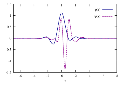
Figure 1: Least asymmetric Daubechies wavelet family of order $2m=16$. Note that both the scaling function $\phi(x)$ and the wavelet $\psi(x)$ are different from zero only within the interval $[1-m,m]$.

Every wavelet family comprises a scaling function $\phi$, and a second function $\psi$ properly called wavelet. Fig. 1 illustrates the least asymmetric Daubechies wavelet family of order $2m=16$, the basis set which is used in the present study. These functions feature a compact support $[1-m,m]$ and are smooth, therefore localized in Fourier space as well.

A basis set is simply generated by the integer translates of the scaling and wavelet functions, with arguments measured in units of the grid spacing $\ell$. For instance, a 1D domain of extension $L$, centered at $x=0$, can be spanned by the following set of $N$ scaling functions,

$$\braket{x}{\phi_{i}}\equiv\phi_{i}(x)=\frac{1}{\sqrt{\ell}}\,\phi\left(\frac{x}{\ell}-i\right),\;i=-N/2,\dots,N/2\,,$$ (7)

where $\ell=L/(N-1)$ is the (uniform) grid spacing. The basis set can be completed by the addition of the translates of the wavelet functions $\psi_{i}$. These functions form a orthogonal basis set:

$$\braket{\phi_{i}}{\phi_{j}}=\delta_{ij}=\braket{\psi_{i}}{\psi_{j}}\,,\quad\braket{\phi_{i}}{\psi_{j}}=0\,.$$ (8)

In three dimensions, a wavelet basis set can easily be obtained as the tensor product of one-dimensional basis functions, combining wavelets and scaling functions along each coordinate of the Cartesian grid (see e.g. Ref. Genovese et al., 2008).

The most important feature of any wavelet basis set is related to the concept of multiresolution. Such a feature builds upon the following scaling equations (or “refinement relations”):

$$\phi(x) = \sqrt{2}\sum_{j}h_{j}\,\phi(2x-j)\,;$$ (9)

$$\psi(x) = \sqrt{2}\sum_{j}g_{j}\,\phi(2x-j)\,,$$ (10)

which relate the wavelet representation at some resolution to that at twice the given resolution, and so on. According to the standard nomenclature, the sets of the $h_{j}$ and $g_{j}=(-1)^{j}h_{1-j}$ coefficients are called low- and high-pass filters, respectively. A wavelet family is therefore completely defined by its low-pass filter. In the case of Daubechies-$2m$ wavelets, $j\in[1-m,m]$.

The representation $f(x)$ of a function in the above defined basis set is given by:

$$f(x)=\sum_{i=-N/2}^{N/2}c_{i}\,\phi_{i}(x)+\sum_{i=-N/2}^{N/2}d_{i}\,\psi_{i}(x)\,,$$ (11)

where the expansion coefficients are formally given by $c_{i}\equiv\braket{\phi_{i}}{f}$, $d_{i}\equiv\braket{\psi_{i}}{f}$. Using the refinement equations (9) and (10), one can map the basis appearing in Eq. (11) to an equivalent one including only scaling functions on a finer grid of spacing $\ell/2$.

The multiresolution property plays a fundamental role also for the wavelet representation of differential operators. For example, it can be shown that the exact matrix elements of the kinetic operator,

$$T_{i-j}\equiv-\frac{1}{2}\int{\rm d}x\,\phi_{i}(x)\partial^{2}\phi_{j}(x)\,,$$ (12)

equal the entries of an eigenvector of a matrix which solely depends on the low-pass filter (see e.g. Ref. Goedecker, 1998). The construction of the kinetic operator $\hat{T}$ in a wavelet basis set does not require any sort of approximation or numerical integration. In the next section, we will show that the matrix elements of $\hat{W}$ can be calculated in a similar way.

The discretization error due to Daubechies-$2m$ wavelets is controlled by the grid spacing. Daubechies-$2m$ wavelets exhibit $m$ vanishing moments, thus any polynomial of degree less than $m$ can be represented exactly by an expansion over the sole scaling functions of order $m$. For higher order polynomials the error is $\mathcal{O}(\ell^{m})$, i.e. vanishingly small as soon as the grid is sufficiently fine. Hence, the difference between the representation of Eq. (11) and the exact function $f$ decreases as $\ell^{m}$. Among all the wavelet families, Daubechies wavelets feature the minimum support length for a given number of vanishing moments.

Given a potential $V$ known numerically on the points $\{x_{k}\}$ of a uniform grid, it is possible to identify an effective approximation for the potential matrix elements $V_{ij}\equiv\bra{\phi_{j}}V\ket{\phi_{i}}$. It has been shown Neelov and Goedecker (2006); Genovese et al. (2008) that a quadrature filter $\{\omega_{k}\}$ can be defined such that the matrix elements given by

$$V_{ij}\equiv\bra{\phi_{j}}V\ket{\phi_{i}}=\sum_{k}\omega_{k-i}\,V(x_{k})\,\omega_{k-j}\,,$$ (13)

yield excellent accuracy with the optimal convergence rate $\mathcal{O}(\ell^{2m})$ for the potential energy. The same quadrature filter can be used to express the grid point values of a (wave)function given its expansion coefficients in terms of scaling functions:

$$f(x_{k}) =\sum_{i}c_{i}\,\omega_{k-i}+\mathcal{O}(\ell^{m})\,;$$ (14)

$$c_{i} =\sum_{k}f(x_{k})\,\omega_{k-i}+\mathcal{O}(\ell^{m})\,.$$ (15)

As a result, the potential energy can equivalently be computed either in real space or in the wavelet space, i.e. $\bra{f}V\ket{f}=\sum_{k}f(x_{k})V(x_{k})f(x_{k})\equiv\sum_{ij}c_{i}V_{ij}c_{j}$. The quadrature filter elements can therefore be considered as the most reliable transformation between grid point values $f(x_{k})$ and scaling function coefficients $c_{i}$, as they provide exact results for polynomials of order up to $m-1$ and do not alter the convergence properties of the basis set discretization. The filter $\{\omega_{k}\}$ is of length $2m$ and is defined unambiguously by the moments of the scaling functions (which in turn depend only on the low-pass filter) Gopinath and Burrus (1992); Johnson et al. (1999).

Using the above formulae, the Hamiltonian matrix $H_{ij}=T_{ij}+V_{ij}$ can be constructed. Note that, in contrast to other discretization schemes (finite differences, DVR, plane waves, etc.), in the wavelet basis set neither the potential nor the kinetic terms have diagonal representations. Instead, $\hat{H}$ is represented by a band matrix of width $4m-1$.

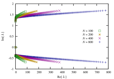
Figure 2: Spectrum of the operator $\hat{W}$ - cf. Eq. (17) - for different sizes $N$ of the basis set. Knowing that the spectrum of $\hat{W}$ is symmetric around the imaginary axis, only the right half-plane is shown.

III Complex Scaling via Similarity Transformation

The complex scaling operator $\hat{S}_{\theta}$ being separable along the three spatial directions, and the wavelet transform of 3D objects being given by the tensor product of three 1D wavelet transforms, it is sufficient to build the complex scaling operator suitable to working on 1D input functions. 3D complex-scaled potentials can thus be obtained through the threefold application of the same 1D operator, each time acting along a different direction:

$$V(x\,e^{\mathrm{i}\theta},y\,e^{\mathrm{i}\theta},z\,e^{\mathrm{i}\theta})=[{\hat{S}_{\theta}}^{x}{\hat{S}_{\theta}}^{y}{\hat{S}_{\theta}}^{z}V](x,y,z)\,.$$ (16)

In what follows, we drop the superscript denoting the spatial direction and focus on the construction of the 1D complex scaling operator, taking

$$\hat{W}=\mathrm{i}(x-x_{0})\frac{\partial}{\partial x}\,.$$ (17)

Owing to the scaling properties of wavelets and scaling functions, the matrix elements $W_{i,j}$ of the operator $\hat{W}$ can be computed exactly. The final result reads as

$$W_{i,j}=\mathrm{i}\left[w_{i-j}+\left(\frac{i+j}{2}-x_{0}\right)d_{i-j}\right]\,.$$ (18)

The definitions of the filter coefficients $\{w_{j}\}$ and $\{d_{j}\}$ are deferred to Appendix A, along with the details of their computation. Let us note that, within the Daubechies-$2m$ family, $W_{i,j}=0$ for any pair $\{i,j\}$ such that $|i-j|>2m-2$. Moreover, being $\hat{W}$ scale-invariant, its spectrum depends only on the size $N$ of the basis set. Fig. 2 shows that the eigenvalues of $\hat{W}$ span a range which reaches a maximum that is $\lesssim N$.

Once the exact wavelet representation of the operator $\hat{W}$ is available, the operator $\hat{S}_{\theta}$ can be represented by its spectral decomposition over the eigenvalues and eigenvectors of $\hat{W}$:

$$\hat{S}_{\theta}=e^{\theta\hat{W}}=\sum_{i=1}^{N}e^{\theta\lambda_{i}}\,|\psi_{\lambda_{i}}\rangle\langle\psi_{\lambda_{i}}|\,,$$ (19)

where $\lambda_{i}$ is the eigenvalue corresponding to the eigenvector $|\psi_{\lambda_{i}}\rangle$. However, special attention has to be paid when using Eq. (19) as is, since numerical instabilities are likely to occur depending on the maximum value attained by $\textrm{Re}(\theta\lambda_{i})$ (in other words: on the condition number of the operator $\hat{S}_{\theta}$). For instance, if the computation is carried out in double-precision floating point arithmetic (by far the most typical case), the relevant terms of the spectral decompositions (19) should lie in the region $10^{-15}<|e^{\theta\lambda_{i}}|<10^{15}$. In order for the complex rotation to be reliable, the scalar product $\langle\psi_{\lambda_{i}}|V\rangle$ should be non-zero only for a subset $\{\lambda_{i}\}$ for which $|e^{\theta\lambda_{i}}|$ falls within the same range. This is however likely to happen, provided the potential $V$ is sufficiently localized in real and reciprocal space. Actually, since the exact eigenfunction of $\hat{W}$ corresponding to the (complex) eigenvalue $\lambda$ is given by $\psi_{\lambda}(x)\propto(x-x_{0})^{-\mathrm{i}\lambda}$, the real part of $\lambda$ can be deemed as a wavenumber in a logarithmic configuration space. Given that $x\,\partial_{x}=-(1+p\,\partial_{p})$, the same behavior would hold also in reciprocal space, $\psi_{\lambda}(p)\propto p^{\mathrm{i}\lambda-1}$. Smooth and localized functions are therefore likely to exhibit non-trivial projections only onto the lowest-lying eigenstates of $\hat{W}$.

At the same time, for two functions $f(x)$ and $g(x)=f(x)+c$ that differ by a global constant $c\in\mathbb{C}$, the equality $\hat{S}_{\theta}g=\hat{S}_{\theta}f+c$ is expected to hold for any $\theta$. The numerical representation of the operator $\hat{S}_{\theta}$ should namely behave as the identity on a generic constant vector $|c\rangle$. A numerically stable implementation should therefore be such that $\langle\psi_{\lambda_{i}}|V\rangle=\langle\psi_{\lambda_{i}}|V+c\rangle$ for any $\lambda_{i}\neq 0$. Such a requirement can be enforced by imposing suitable boundary conditions on the matrix elements of $\hat{W}$, as demonstrated by the following result, which involves the $n$-th moment of a generic left-eigenfunction $\psi_{\lambda}(x)$ of $\hat{W}$ (assuming $x_{0}=0$, $\lambda\psi_{\lambda}(x)\equiv\psi_{\lambda}(x)\overleftarrow{W}=\mathrm{i}\,\partial_{x}\left[x\,\psi_{\lambda}(x)\right]$):

$$(\lambda+\mathrm{i}\,n)\int_{-L/2}^{L/2}{\rm d}x\,\psi_{\lambda}(x)x^{n}=\\ \mathrm{i}\left(\frac{L}{2}\right)^{n+1}\left[\psi_{\lambda}(L/2)+(-1)^{n}\psi_{\lambda}(-L/2)\right]\;.$$ (20)

In particular, for $n=0$ the boundary term on the right hand side becomes zero if $\psi_{\lambda}(L/2)=-\psi_{\lambda}(-L/2)$, and $\langle\psi_{\lambda}|c\rangle\leavevmode\nobreak\ =\leavevmode\nobreak\ 0$ for any $\lambda\neq 0$. In other words, the only left-eigenvector of $\hat{W}$ that has a non-trivial projection on a constant, is the one corresponding to the zero eigenvalue. Such boundary conditions can be imposed by setting

$$W_{i,j\pm N}=-\mathrm{i}\left[w_{i-j}+\left(\frac{i+j}{2}-x_{0}\right)d_{i-j}\right]\,.$$ (21)

The zero eigenvalue can actually be found in the spectrum of the $\hat{W}$ operator that is so obtained (see Fig. 2), the pair matching right-eigenvector being identically constant.

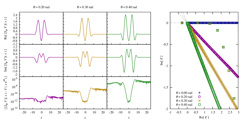
Figure 3: Left: the results of the application of the wavelet-based complex scaling method to the potential (29) for different complex scaling angles. In the bottom row, we plot the absolute value of the difference between the exact complex-scaled potential $V(xe^{\mathrm{i}\theta})$ and that obtained through similarity transformation in the wavelet basis set, $[\hat{S}_{\theta}V](x)$. Right: the low-energy portion of the spectrum of the corresponding complex-scaled Hamiltonian. One can note that continuum states align along rays (dot-dashed straight lines in the plot) that are rotated by $2\theta$ with respect to the real axis, while bound and resonant states can be identified by the fact that they do not depend on $\theta$.

IV The Complex Virial Theorem

As a result of the Balslev-Combes theorem Balslev and Combes (1971), bound and resonant eigenstates are expected to be stationary with respect to variations of the complex scaling angle $\theta$. Moreover, the complex analog of the Hellmann-Feynmann theorem Moiseyev (2011) allows to relate the variation of the $i$-th eigenvalue $E^{(i)}$ with respect to $\theta$ (considered as a variational parameter) to the quantum expectation value of $\partial\hat{H}_{\theta}/\partial\theta$ on the corresponding eigenstate $|{\psi_{\theta}^{(i)}})$:

$$\frac{{\rm d}E^{(i)}}{{\rm d}\theta}=\left(\psi_{\theta}^{(i)}\right|\frac{\partial\hat{H}_{\theta}}{\partial\theta}\left|\psi_{\theta}^{(i)}\right),$$ (22)

being

$$E^{(i)}=\frac{(\psi_{\theta}^{(i)}|\hat{H}_{\theta}|\psi_{\theta}^{(i)})}{(\psi_{\theta}^{(i)}|\psi_{\theta}^{(i)})}\;.$$ (23)

Given the definition of $\hat{H}_{\theta}$ in Eq. (4), it is easy to show that

$$\frac{\partial\hat{H}_{\theta}}{\partial\theta}=[\hat{W},\hat{H}_{\theta}]\,,$$ (24)

and to rephrase the requirement of $\theta$-independence in terms of the complex virial theorem (CVT):

$$\frac{{\rm d}E^{(i)}}{{\rm d}\theta}=0\Longleftrightarrow(\psi_{\theta}^{(i)}|[\hat{W},\hat{H}_{\theta}]|\psi_{\theta}^{(i)})=0\,.$$ (25)

As shown e.g. in Ref. Rice et al., 1996 it is possible to prove that

$$[\hat{W},\hat{H}_{\theta}]=-2\mathrm{i}\,(\hat{T}_{\theta}+\hat{U}_{\theta})\,,$$ (26)

where

$$\hat{U}\equiv-\frac{x-x_{0}}{2}\frac{\partial\hat{V}}{\partial x}=\frac{\mathrm{i}}{2}\hat{W}\hat{V}\,.$$ (27)

Eventually, the virial theorem reads as follows:

$$\left(\psi^{(i)}_{\theta}\right|\hat{T}_{\theta}+\hat{U}_{\theta}\left|\psi^{(i)}_{\theta}\right)=0\,.$$ (28)

When using finite basis sets, the condition (28) may not be satisfied, or be satisfied to a great extent only within certain intervals of the angle $\theta$. Such an occurrence is extensively reported in the literature Yaris and Winkler (1978). Resonant eigenvalues have been shown to move along the so-called $\theta$-trajectories in the complex plane as $\theta$ is varied, the features of which (cusps, in particular) can be used to assess the level of convergence towards stationary points, and might hint at the selection of the optimal complex scaling angle Moiseyev et al. (1981, 1978); Moiseyev and Corcoran (1979).

The evaluation of ${\rm d}E^{(i)}/{\rm d}\theta$ thus represents an assessment of the degree of convergence towards true bound and resonant states in numerical computations with finite basis sets. A closer look at Eq. (27) reveals that no additional effort is required to obtain the operator $\hat{U}$ in the wavelet basis set, once $\hat{W}$ has been generated. Moreover, the complex-scaled counterpart $\hat{U}_{\theta}$ can be obtained by acting on $\hat{U}$ with the complex scaling operator $\hat{S}_{\theta}$, exactly as if $\hat{U}$ were a generic potential operator.

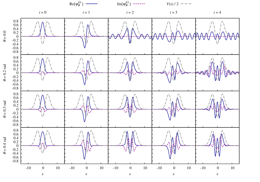
Figure 4: Complex-rotated $c$-normalized eigenfunctions corresponding to the five lowest-lying eigenstates (from left to right: one bound state and four resonant states), computed at $\theta=\{0,0.2,0.3,0.4\}\;\mbox{rad}$. Solid (dashed) lines correspond to the real (imaginary) part of the eigenfunctions. Dot-dashed lines represent the potential (rescaled by a numerical factor), which is superimposed so to highlight the localization of the complex-rotated eigenfunctions inside the interaction region.

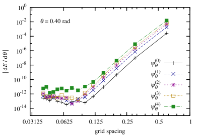
Figure 5: Measurement of the fulfillment degree of the complex virial theorem, Eq. (28). The result of the evaluation of Eq. (28) is shown as a function of the grid spacing of the simulation domain, for the five lowest-lying states of the complex-scaled Hamiltonian at $\theta=0.4\;\textrm{rad}$ obtained through similarity transformation in the Daubechies-16 wavelet basis set. The potential is that of Eq. (29).

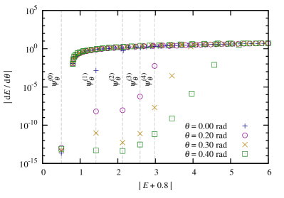
Figure 6: The results obtained for $\hat{H}_{\theta}$ with the potential as from Eq. (29), with a focus on the low-energy end. The grid spacing was set equal to $0.075$ (cf. Fig. 5). The offset $0.8$ ($=-V(x=0)$) was added to the eigenenergies in order to avoid ambiguities in the ordering of states, even in terms of the absolute values of the associated eigenenergies. Vertical dashed lines are superimposed on the eigenenergies of the five lowest-lying discrete states.

V Illustrative examples

In order to validate our wavelet approach to complex scaling via similarity transformation, we first discuss the application of our method to a specific 1D model potential. We chose to work on the following potential,

$$V(x)=\left(\frac{1}{2}x^{2}-a\right)e^{-\lambda x^{2}}+E_{\textrm{th}}\,,$$ (29)

with $a=0.8$, $\lambda=0.1$ and $E_{\textrm{th}}=0$, because the same potential, with $E_{\textrm{th}}=0.8$, has been thoroughly studied in the literature, hence we could cross-check our results against the already published ones. Let us point out that we do not aim to provide new information concerning the resonances exhibited by the model potential (29), instead to show that 1. the wavelet-based complex scaling transformation is extremely accurate; 2. the finite wavelet basis set computation of resonant states yields very good figures of the fulfillment of the CVT.

The potential (29), which models diatomic molecular pre-dissociation resonances, has already been studied in a number of publications, namely in Refs. Moiseyev et al., 1978, 1984 (adopting a Gaussian basis set), in Refs. Rittby et al., 1981, 1982 (employing Weyl’s theory and the direct numerical integration of the complex-rotated Schrödinger equation under Siegert boundary conditions), in Refs. Korsch et al., 1982a, b (employing a non-Hermitian generalization of the Milne’s method), in Ref. Moiseyev, 1998b (using a complex absorbing potential and plane waves as basis functions) and in Refs. Museth and Leforestier, 1996; Bludský et al., 1998; Leforestier and Museth, 1998; Fang and Mei-Shan, 2008a, b (using the sine DVR). More specifically, in Refs.  Fang and Mei-Shan, 2008a, b the potential is complex-scaled while the basis functions are not; in Refs.  Museth and Leforestier, 1996, Bludský et al., 1998 and Leforestier and Museth, 1998 the basis functions are scaled, but not the potential. The model potential (29) exhibits only one bound state (at $E-E_{\textrm{th}}\simeq-0.3$), and several resonant states.

The outcome of the complex scaling operation applied to the potential (29) is shown in Fig. 3, together with a comparison against the exact complex-scaled potential. An excellent agreement is found throughout the spatial range for all the values of $\theta$.

The full diagonalization of the complex-scaled Hamiltonian obtained through similarity transformation provides a further confirmation of the reliability of the wavelet-based complex scaling operation. To this effect we show, in the right panel of Fig. 3, the low-energy region of the $\hat{H}_{\theta}$ spectrum and, in Fig. 4, the eigenfunctions of the five lowest-lying states (one bound state and four resonances). It can be observed that resonant eigenfunctions are well localized inside the interaction region and well-behaved throughout the spatial range, pretty much like a bound state. The localization increases while increasing the complex scaling angle (the effect being more evident for the resonances at higher energy). Also shown are the eigenfunctions sorted out from the spectrum of $\hat{H}_{\theta=0}$ by looking up the eigenvalues which were the closest to the resonant eigenvalues computed at $\theta>0$.

In Fig. 5, the rates of convergence towards true resonant states (namely, the degree of fulfillment of the CVT) are displayed. The rates improve upon decreasing the grid spacing, as a consequence of the systematicity of Daubechies wavelets. In the case of a sufficiently fine grid, the figures of the violation of the CVT become as little as $\lesssim 10^{-11}$, for all five lowest-lying states. Such figures have to be compared with those referring to continuum states ($\gtrsim 10^{-2}$, see Fig. 6). The gap of several orders of magnitude between bound/resonant states and continuum states allows to easily distinguish the former from the latter within the $\hat{H}_{\theta}$ spectrum. It is also interesting to note how the measure of the violation of the CVT changes vs $\theta$ for the different resonances.

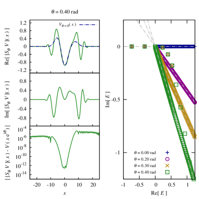
Figure 7: The result of the wavelet-based complex scaling as applied through similarity transformation to an illustrative multi-centered potential $V(x)=0.25\exp[-0.1(x-7.5)^{2}]+0.5\exp[-0.1(x+5)^{2}]-\exp(-0.1x^{2})$. Left: real (top) and imaginary (center) part of the complex-scaled potential at $\theta=0.4\;\textrm{rad}$, and comparison (bottom) against the exact result. Right: low-energy portion of the spectrum of the corresponding non-Hermitian Hamiltonian. By virtue of the $\theta$-independence one can identify a pair of bound states and a number of resonances.

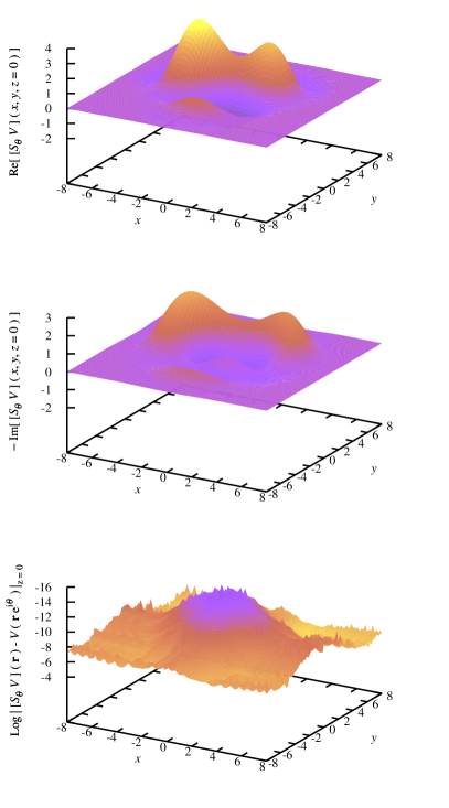
Figure 8: The result of the wavelet-based complex scaling applied to a fictitious 3D potential, $V(\vec{r})=\sum_{k=0}^{3}a_{k}e^{-\beta_{k}|\vec{r}-\vec{r}_{k}|^{2}}$ with $a_{0}=-3$, $a_{1}=2$, $a_{2}=4$, $a_{3}=3$, $\beta_{0}=0.1$, $\beta_{1}=\beta_{2}=\beta_{3}=0.2$, $\vec{r}_{0}=0$, $\vec{r}_{1}=3(0,-1,1/2)$, $\vec{r}_{2}=3/2(-\sqrt{3},1,0)$, $\vec{r}_{3}=3/2(1,\sqrt{3},0)$ and $\theta=0.3\;\textrm{rad}$: 2D surfaces at $z=0$ representing the real (top), imaginary (center) part of $[\hat{S}_{\theta}V](r)$ and the discrepancy (bottom) from the exact result. Note that, for better visibility, the opposite of the imaginary part is plotted.

We wish now to discuss the results obtained upon applying the method to a multi-centered one-dimensional potential (Fig. 7) and to a 3D potential (Fig. 8), with the twofold aim of providing evidence that the method also works in three dimension and that no special restrictions have to be imposed on the symmetry of the potential. While referring to the figure caption for further information on the shape of the two potentials, we wish to remark that the wavelet-based complex scaling method proves to be, once again, very accurate.

We look forward to applying the wavelet-based complex scaling method to genuine ab initio potentials, as a first crucial step towards resonances in realistic 3D (isolated) systems.

VI Conclusion

We have shown that the adoption of wavelets as a basis set allows to implement the complex scaling method via similarity transformation in a rigorous and effective way. Since wavelets display well-defined transformation properties upon rescaling of the spatial coordinates, they are especially well-suited for the discretization of scale-invariant operators such as the complex scaling generator $\hat{W}$. In addition, the localization of wavelets (both in real and reciprocal space) allows to represent complex scaling transformation through the spectral decomposition over the eigenstates of a matrix that is inherently band-like. As a consequence, no artificial convergence parameter has to be introduced.

By testing the method on a host of 1D and 3D model potentials, we were able to prove that our implementation is also very accurate. This general technique, starting from the numerical values $\{f(x_{k})\}$ of a generic function $f(x)$ on a (uniform) real space grid, computes the values $\{f(x_{k}e^{\mathrm{i}\theta})\}$ by performing a similarity transformation in the Daubechies wavelets basis set. The output may be further processed in any other basis set of choice, e.g. for the extraction of resonant states of the complex-scaled Hamiltonian.

By carrying out a resonant state computation in the case of a one-dimensional model system, we were able to demonstrate that our approach exhibit excellent convergence rate in terms of the size of the basis set. The violation of the complex virial theorem can become comparable to the machine precision, hence totally negligible.

Resonant states are supposed to provide a concise description of one-particle excitations, meaning that a certain energy range ought to be spanned by a few resonant states rather than a virtually infinite set of continuum states. It has been claimed, for instance, that “one can construct the Green function simply in the form of a sum over the Siegert states, avoiding the annoying integral over the continuum.” (citation from Ref. Tolstikhin et al., 1997; see also Refs. Hatano, 2010; Hatano and Ordonez, 2011). Several other investigations indicate the possibility of describing scattering cross sections, optical absorption spectra et cetera by means of a collection of purely discrete (bound and resonant) states Myo et al. (1998). Nevertheless, the very numerical computation of resonant states is a formidable challenge. In our study, we showed that wavelets allow obtaining a complex-scaled Hamiltonian which can contain resonant states in its spectrum (if any). Irrespectively of the basis set in which one wishes to further the computation, in realistic numerical simulations the size of the Hamiltonian matrix can be so large that the full diagonalization becomes practically unaffordable. Moreover, one has to cope with the fact that, within the framework of non-Hermitian quantum mechanics, the variational principle states that “true” states are only stationary points along the variational trajectories (instead of minima). Hence, methods that are already in use for the computation of bound states cannot be deployed as such.

A crucial achievement toward the numerical computation of resonant states should regard the development of clever techniques for their direct extraction, allowing to focus on selected sub-regions of the spectrum of the non-Hermitian Hamiltonian (like, for instance, the filter diagonalization method Santra and Cederbaum (2002)). Work is in progress in this direction. We also look forward to carrying out computations in the frame of many-body perturbation theory with the inclusion of resonant states Whitenack (2012), hoping to be able to shed new light on the theoretical description of optical and electronic excitations. To this respect, the present study represents a first essential step, since it opens up the possibility of obtaining the complex-scaled version of Hamiltonians based on 3D ab initio potentials.

Appendix A Representation of the $\hat{W}$ operator in a wavelet basis set

Computing the wavelet representation of the operator $\hat{W}$ - cf. Eq. (17) - amounts to evaluating the following matrix elements:

$$W^{(00)}_{m,n} \equiv \int_{\mathbb{R}}{\rm d}x\,\phi_{m}(x)\hat{W}\phi_{n}(x)\;;$$ (30a)

$$W^{(01)}_{m,n} \equiv \int_{\mathbb{R}}{\rm d}x\,\phi_{m}(x)\hat{W}\psi_{n}(x)\;;$$ (30b)

$$W^{(10)}_{m,n} \equiv \int_{\mathbb{R}}{\rm d}x\,\psi_{m}(x)\hat{W}\phi_{n}(x)\;;$$ (30c)

$$W^{(11)}_{m,n} \equiv \int_{\mathbb{R}}{\rm d}x\,\psi_{m}(x)\hat{W}\psi_{n}(x)\;,$$ (30d)

where $\phi_{i}(x)\equiv\phi(x-i)$ and $\psi_{i}(x)\equiv\psi(x-i)$ are the scaling function and the wavelet belonging to a wavelet family, respectively. In our specific implementation, we adopted Daubechies wavelets, for the reasons outlined in Sec. II. Introducing the following variables,

$$I\equiv\frac{m+n}{2}\,,\qquad J\equiv\frac{m-n}{2}\,,$$ (31)

and switching from $x$ to $x^{\prime}=x-I$, we can split $W^{(00)}_{m,n}$ into a translation-invariant part, which indeed depends only on $J$, and a non-translation-invariant part. Eventually,

$$W^{(00)}_{m,n}=\mathrm{i}\left[w^{(00)}_{m-n}+\left(\frac{m+n}{2}-x_{0}\right)\,d^{(00)}_{m-n}\right]\,,$$ (32)

where

$$w^{(00)}_{i}\equiv\int_{\mathbb{R}}{\rm d}x\,\phi(x-i/2)\,x\frac{\partial}{\partial x}\,\phi(x+i/2)$$ (33)

and

$$d_{i}^{(00)}\equiv\int_{\mathbb{R}}{\rm d}x\,\phi(x-i)\frac{\partial}{\partial x}\phi(x)=-d_{-i}^{(00)}\,.$$ (34)

The last equality is a consequence of the scaling functions and wavelets’ compact support. The results for $W^{(01)}_{m,n}$, $W^{(10)}_{m,n}$, $W^{(11)}_{m,n}$ follow analogously, provided that in the preceding equations we change $\phi(x)\rightarrow\psi(x)$ and $0\rightarrow 1$ according to Eqs. (30).

The entries of the vector $d^{(00)}$ can be computed following the steps outlined in Ref. Goedecker, 1998 (Section 23), namely by exploiting the scaling equation featured by scaling functions and wavelets, Eqs. (9-10). Thanks to the localization of scaling functions, the number of non-trivial $d_{j}^{(00)}$’s amounts to just a few: $d_{j}^{(00)}\neq 0\Leftrightarrow|j|\leq 2m-2$, where $m$ is the order of the Daubechies wavelet family. The same holds for the other $d$ vectors, which, as a further consequence of Eqs. (9-10), can be computed as follows:

$$d_{i}^{(01)}=2\sum_{\mu,\nu}h_{\mu}\,g_{\nu}\,d^{(00)}_{2i+\mu-\nu}\;;$$ (35a)

$$d_{i}^{(10)}=2\sum_{\mu,\nu}g_{\mu}\,h_{\nu}\,d^{(00)}_{2i+\mu-\nu}\;;$$ (35b)

$$d_{i}^{(11)}=2\sum_{\mu,\nu}g_{\mu}\,g_{\nu}\,d^{(00)}_{2i+\mu-\nu}\;,$$ (35c)

where $\{h_{\mu}\}_{\mu\in[1-m,m]}$, $\{g_{\mu}\}_{\mu\in[1-m,m]}$ are the low- and high-pass filters, respectively (cf. Sec. II).

The entries of the vector $w^{(00)}$ can instead be computed as explained below, where $M\equiv(\mu+\nu)/2$, $N\equiv(\mu-\nu)/2$, and the scaling relation Eq. (9) is used:

$$w^{(00)}_{J} = 2\sum_{\mu,\nu}h_{\mu}h_{\nu}\int{\rm d}x\,\phi(2x-J-\mu)\,x\frac{\partial}{\partial x}\,\phi(2x+J-\nu)$$ (36a)

$$= 2\sum_{M,N}h_{M+N}h_{M-N}\int{\rm d}x\,\phi(2x-J-M-N)\,x\frac{\partial}{\partial x}\,\phi(2x+J-M+N)$$ (36b)

$$= \sum_{M,N}h_{M+N}h_{M-N}\int{\rm d}x\,\phi(x-J-N)\,(x+M)\frac{\partial}{\partial x}\,\phi(x+J+N)$$ (36c)

$$= \sum_{M,N}h_{M+N}h_{M-N}\left[w^{(00)}_{2(J+N)}+Md^{(00)}_{2(J+N)}\right]\,.$$ (36d)

Integrating by parts Eq. (33), it is easy to prove that

$$w^{(00),(11)}_{j} = -w^{(00),(11)}_{-j}-\delta_{j,0}\;;$$ (37a)

$$w^{(01)}_{j} = -w^{(10)}_{-j}\;,$$ (37b)

and, as a corollary, that $w^{(00)}_{0}=-1/2=w^{(11)}_{0}$. Moreover, $|j|>2m-2\Rightarrow w^{(00),(01),(10),(11)}_{j}=0$. Restoring the original indexes $\mu,\nu$ in (36d), and rearranging terms in a convenient way, we are left with

$$\sum_{k}A_{J,k}\,w^{(00)}_{k}=b_{J}\,,$$ (38)

where

$$A_{J,k}\equiv\delta_{J,k}-\sum_{\mu,\nu}h_{\mu}\,h_{\nu}\,\delta_{\mu-\nu+2J,k}$$ (39)

and

$$b_{J}\equiv\sum_{\mu,\nu}h_{\mu}\,h_{\nu}\,\frac{\mu+\nu}{2}\,d^{(00)}_{\mu-\nu+2J}\,.$$ (40)

Namely, the entries of $w^{(00)}$ can be found as the solution of the linear system of equations (38), which is neither under- nor over-determined. Formally equivalent linear systems, although with different numerical coefficients, lead to the solution for the vectors $w^{(01)}$, $w^{(10)}$, $w^{(11)}$. For instance, $w^{(01)}$ is the solution of

$$\sum_{k}A^{\prime}_{J,k}\,w^{(01)}_{k}=b^{\prime}_{J}\,,$$ (41)

with

$$A^{\prime}_{J,k}\equiv\delta_{J,k}-\sum_{\mu,\nu}h_{\mu}\,g_{\nu}\,\delta_{\mu-\nu+2J,k}$$ (42)

and

$$b^{\prime}_{J}\equiv\sum_{\mu,\nu}h_{\mu}\,g_{\nu}\,\frac{\mu+\nu}{2}\,d^{(01)}_{\mu-\nu+2J}\,.$$ (43)

References

- Hatano (2010) N. Hatano, Progress of Theoretical Physics Supplement 184, 497 (2010), URL http://ptp.ipap.jp/link?PTPS/184/497/.
- Siegert (1939) A. J. F. Siegert, Phys. Rev. 56, 750 (1939), URL http://link.aps.org/doi/10.1103/PhysRev.56.750.
- Aguilar and Combes (1971) J. Aguilar and J. M. Combes, Communications in Mathematical Physics 22, 269 (1971), ISSN 0010-3616, URL http://dx.doi.org/10.1007/BF01877510.
- Balslev and Combes (1971) E. Balslev and J. M. Combes, Communications in Mathematical Physics 22, 280 (1971), URL http://www.springerlink.com/index/R46314PT83439W82.pdf.
- Simon (1972) B. Simon, Communications in Mathematical Physics 27, 1 (1972), ISSN 0010-3616, 10.1007/BF01649654, URL http://dx.doi.org/10.1007/BF01649654.
- Moiseyev (2011) N. Moiseyev, Non-Hermitian Quantum Mechanics (Cambridge University Press, 2011), ISBN 9780521889728.
- Moiseyev (1998a) N. Moiseyev, Physics Reports 302, 212 (1998a), ISSN 0370-1573, URL http://www.sciencedirect.com/science/article/pii/S0370157398000027.
- Klaiman and Moiseyev (2010) S. Klaiman and N. Moiseyev, Journal of Physics B: Atomic, Molecular and Optical Physics 43, 185205 (2010), ISSN 0953-4075, URL http://stacks.iop.org/0953-4075/43/i=18/a=185205?key=crossref.de6cb43c2783dbfb9b75d2082cb7737a.
- Junker (1982) B. R. Junker (Academic Press, 1982), vol. 18, chap. Advances in Atomic and Molecular Physics, pp. 207–263, URL http://www.sciencedirect.com/science/article/pii/S0065219908602420.
- Reinhardt (1982) W. P. Reinhardt, Annual Review of Physical Chemistry 33, 223 (1982), URL http://www.annualreviews.org/doi/abs/10.1146/annurev.pc.33.100182.001255.
- Ho (1983) Y. K. Ho, Physics Reports 99, 1 (1983), ISSN 0370-1573, URL http://www.sciencedirect.com/science/article/pii/0370157383901126.
- Moiseyev (1984) N. Moiseyev, in Resonances – Models and Phenomena, edited by S. Albeverio, L. Ferreira, and L. Streit (Springer Berlin Heidelberg, 1984), vol. 211 of Lecture Notes in Physics, pp. 235–256, ISBN 978-3-540-13880-8, URL http://dx.doi.org/10.1007/3-540-13880-3_76.
- Moiseyev and Corcoran (1979) N. Moiseyev and C. Corcoran, Phys. Rev. A 20, 814 (1979), URL http://link.aps.org/doi/10.1103/PhysRevA.20.814.
- Ryaboy and Moiseyev (1995) V. Ryaboy and N. Moiseyev, The Journal of Chemical Physics 103, 4061 (1995), ISSN 00219606, URL http://link.aip.org/link/JCPSA6/v103/i10/p4061/s1&Agg=doi.
- Museth and Leforestier (1996) K. Museth and C. Leforestier, The Journal of Chemical Physics 104, 7008 (1996), URL http://link.aip.org/link/?JCP/104/7008/1.
- Moiseyev and Hirschfelder (1988) N. Moiseyev and J. O. Hirschfelder, The Journal of Chemical Physics 88, 1063 (1988), ISSN 00219606, URL http://link.aip.org/link/JCPSA6/v88/i2/p1063/s1&Agg=doi.
- Mandelshtam and Moiseyev (1996) V. A. Mandelshtam and N. Moiseyev, The Journal of Chemical Physics 104, 6192 (1996), URL http://link.aip.org/link/?JCP/104/6192/1.
- Goedecker (1998) S. Goedecker, Wavelets and their application for the solution of partial differential equations in physics (Presses Polytechniques et Universitaires Romandes, Lausanne, Switzerland, 1998), ISBN 2-88074-398-2.
- Daubechies (1992) I. Daubechies, Ten lectures on wavelets, vol. 61 of CBMS-NSF Regional Conference Series in Applied Mathematics (Society for Industrial and Applied Mathematics (SIAM), Philadelphia, PA, 1992), URL http://www.ams.org/mathscinet-getitem?mr=1162107.
- Genovese et al. (2008) L. Genovese, A. Neelov, S. Goedecker, T. Deutsch, S. A. Ghasemi, A. Willand, D. Caliste, O. Zilberberg, M. Rayson, A. Bergman, et al., The Journal of Chemical Physics 129, 014109 (pages 14) (2008), URL http://link.aip.org/link/?JCP/129/014109/1.
- Neelov and Goedecker (2006) A. I. Neelov and S. Goedecker, Journal of Computational Physics 217, 312 (2006), ISSN 0021-9991, URL http://www.sciencedirect.com/science/article/pii/S002199910600012X.
- Gopinath and Burrus (1992) R. Gopinath and C. Burrus, in Proceedings of IEEE International Symposium on Circuits and Systems (1992), vol. 2, pp. 963–966.
- Johnson et al. (1999) B. R. Johnson, J. P. Modisette, P. J. Nordlander, and J. L. Kinsey, The Journal of Chemical Physics 110, 8309 (1999), URL http://link.aip.org/link/?JCP/110/8309/1.
- Rice et al. (1996) S. A. Rice, S. Jang, and M. Zhao, The Journal of Physical Chemistry 100, 11893 (1996), eprint http://pubs.acs.org/doi/pdf/10.1021/jp9607881, URL http://pubs.acs.org/doi/abs/10.1021/jp9607881.
- Yaris and Winkler (1978) R. Yaris and P. Winkler, Journal of Physics B: Atomic and Molecular Physics 11, 1475 (1978), URL http://stacks.iop.org/0022-3700/11/i=8/a=018.
- Moiseyev et al. (1981) N. Moiseyev, S. Friedland, and P. R. Certain, The Journal of Chemical Physics 74, 4739 (1981), URL http://link.aip.org/link/?JCP/74/4739/1.
- Moiseyev et al. (1978) N. Moiseyev, P. R. Certain, and F. Weinhold, Molecular Physics 36, 1613 (1978), URL http://www.tandfonline.com/doi/abs/10.1080/00268977800102631.
- Moiseyev et al. (1984) N. Moiseyev, P. Froelich, and E. Watkins, The Journal of Chemical Physics 80, 3623 (1984), URL http://link.aip.org/link/?JCP/80/3623/1.
- Rittby et al. (1981) M. Rittby, N. Elander, and E. Brändas, Phys. Rev. A 24, 1636 (1981), URL http://link.aps.org/doi/10.1103/PhysRevA.24.1636.
- Rittby et al. (1982) M. Rittby, N. Elander, and E. Brändas, Phys. Rev. A 26, 1804 (1982), URL http://link.aps.org/doi/10.1103/PhysRevA.26.1804.
- Korsch et al. (1982a) H. J. Korsch, H. Laurent, and R. Mohlenkamp, Journal of Physics B: Atomic and Molecular Physics 15, 1 (1982a), URL http://stacks.iop.org/0022-3700/15/i=1/a=008.
- Korsch et al. (1982b) H. J. Korsch, H. Laurent, and R. Möhlenkamp, Phys. Rev. A 26, 1802 (1982b), URL http://link.aps.org/doi/10.1103/PhysRevA.26.1802.
- Moiseyev (1998b) N. Moiseyev, Journal of Physics B: Atomic, Molecular and Optical Physics 31, 1431 (1998b), URL http://stacks.iop.org/0953-4075/31/i=7/a=009.
- Bludský et al. (1998) O. Bludský, Y. Li, G. Hirsch, and R. J. Buenker, The Journal of Chemical Physics 109, 1201 (1998), URL http://link.aip.org/link/?JCP/109/1201/1.
- Leforestier and Museth (1998) C. Leforestier and K. Museth, The Journal of Chemical Physics 109, 1203 (1998), URL http://link.aip.org/link/?JCP/109/1203/1.
- Fang and Mei-Shan (2008a) Z. Fang and Z. Mei-Shan, Communications in Theoretical Physics 49, 599 (2008a), URL http://stacks.iop.org/0253-6102/49/i=3/a=16.
- Fang and Mei-Shan (2008b) Z. Fang and Z. Mei-Shan, Communications in Theoretical Physics 49, 607 (2008b), URL http://stacks.iop.org/0253-6102/49/i=3/a=17.
- Tolstikhin et al. (1997) O. I. Tolstikhin, V. N. Ostrovsky, and H. Nakamura, Phys. Rev. Lett. 79, 2026 (1997), URL http://link.aps.org/doi/10.1103/PhysRevLett.79.2026.
- Hatano and Ordonez (2011) N. Hatano and G. Ordonez, International Journal of Theoretical Physics 50, 1105 (2011), ISSN 0020-7748, URL http://www.springerlink.com/index/10.1007/s10773-010-0576-y.
- Myo et al. (1998) T. Myo, A. Ohnishi, and K. Katō, Progress of Theoretical Physics 99, 801 (1998), URL http://ptp.ipap.jp/link?PTP/99/801/.
- Santra and Cederbaum (2002) R. Santra and L. S. Cederbaum, Physics Reports 368, 1 (2002), ISSN 0370-1573, URL {http://www.sciencedirect.com/science/article/pii/S0370157302001436}.
- Whitenack (2012) D. Whitenack, Annalen der Physik 524, 814 (2012), ISSN 1521-3889, URL http://dx.doi.org/10.1002/andp.201200062.