A theory for the emergence of coherent structures in beta-plane turbulence

Abstract

Planetary turbulent flows are observed to self-organize into large scale structures such as zonal jets and coherent vortices. One of the simplest models of planetary turbulence is obtained by considering a barotropic flow on a beta-plane channel with turbulence sustained by random stirring. Non-linear integrations of this model show that as the energy input rate of the forcing is increased, the homogeneity of the flow is broken with the emergence of non-zonal, coherent, westward propagating structures and at larger energy input rates by the emergence of zonal jets. We study the emergence of non-zonal coherent structures using a non-equilibrium statistical theory, Stochastic Structural Stability Theory (S3T, previously referred to as SSST). S3T directly models a second order approximation to the statistical mean turbulent state and allows identification of statistical turbulent equilibria and study of their stability. Using S3T, the bifurcation properties of the homogeneous state in barotropic beta-plane turbulence are determined. Analytic expressions for the zonal and non-zonal large scale coherent flows that emerge as a result of structural instability are obtained. Through numerical integrations of the S3T dynamical system, it is found that the unstable structures equilibrate at finite amplitude. Numerical simulations of the nonlinear equations confirm the characteristics (scale, amplitude and phase speed) of the structures predicted by S3T.

1 Introduction

Atmospheric and oceanic turbulence is commonly observed to be organized into spatially and temporally coherent structures such as zonal jets and coherent vortices. Examples from planetary turbulence include the banded jets and the Great Red Spot in the Jovian atmosphere (Ingersoll, 1990; Vasavada & Showman, 2005), as well as the latent jets in the Earth’s ocean basins (Maximenko et al., 2005) and the ocean rings shed by the meandering of the Gulf-Stream in the western Atlantic Ocean (Chelton et al., 2007). Laboratory experiments and numerical simulations of both decaying and forced turbulence have shown that these coherent structures appear and persist for a very long time despite the presence of eddy mixing (Vallis & Maltrud, 1993; Cho & Polvani, 1996; Weeks et al., 1997; Read et al., 2004; Espa et al., 2010; Di Nitto et al., 2013).

One of the simplest models of planetary turbulence, is the stochastically forced barotropic vorticity equation on the surface of a rotating planet or on a $\beta$-plane (a plane tangent to the surface of the planet in which differential rotation is taken into account). A large number of numerical simulations of this model have shown that robust, large scale zonal jets emerge in the flow and are sustained at finite amplitude (Williams, 1978; Vallis & Maltrud, 1993; Nadiga, 2006; Danilov & Gurarie, 2004; Galperin et al., 2006). In addition, large scale westward propagating coherent waves were found to coexist with the zonal jets (Sukariansky et al., 2008; Galperin et al., 2010). These waves were found to either obey a Rossby wave dispersion, or propagate with different phase speeds. The propagating waves typically have low zonal wavenumbers and were found in a parameter regime in which strong, robust jets dominate. These waves that are referred to as satellite modes (Danilov & Gurarie, 2004) or zonons (Sukariansky et al., 2008), appear to be sustained by non-linear interactions between Rossby waves. However the mechanism for their excitation and maintenance remains elusive. The goal in this work is to develop a non-equilibrium statistical theory that can predict the emergence of both zonal jets and non-zonal coherent structures and can capture their characteristics.

The tendency for formation of large scale structures in planetary turbulence can be understood in terms of the approximate energy and vorticity conservation in two dimensional or quasi two dimensional flows that implies an energy transfer from small to large scales given that there is a direct enstrophy cascade to small scales (Fjörtöft, 1953). Rhines (1975) found that the non-linear eddy-eddy interactions that are local in wavenumber space, lead to an inverse energy cascade that is anisotropic, as it is inhibited in the region in wavenumber space in which weakly interacting Rossby-waves dominate. The cascade therefore continues through a narrow region in wavenumber space, transferring energy to zonal jets (Vallis & Maltrud, 1993; Nazarenko & Quinn, 2009) and is finally arrested at a meridional scale that is dictated by friction (Smith et al., 2002; Sukariansky et al., 2007). However, observations of the atmospheric midlatitude jet (Shepherd, 1987) and numerical analysis of simulations (Nozawa & Yoden, 1997; Huang & Robinson, 1998; Huang et al., 2001), showed that the large scale jets are maintained through spectrally non-local interactions rather than by a local in wavenumber space cascade. Theoretical studies (Farrell & Ioannou, 2003, 2007) and numerical simulations (Srinivasan & Young, 2012; Constantinou et al., 2013) have also shown that jets emerge even in the absence of cascades. Moreover, the persistence and dominance of specific non-zonal coherent structures that also emerge cannot be explained by the phenomenological description of the inverse turbulent cascade.

Since organization of turbulence into coherent structures involves complex non-linear interactions among a large number of degrees of freedom, an alternative approach for gaining an understanding for the tendency towards self-organization of turbulent flows is to use statistical mechanics, an approach pioneered by Miller (1990) and Robert & Sommeria (1991) in what is now known as Robert-Sommeria-Miller (RSM) theory. The RSM theory builds upon the work of Onsager (1949) that explains self-organization of turbulence in terms of the equilibrium statistical mechanics of a set of point vortices. The main idea is to find a solution of the unforced Euler equations that maximizes a proper measure of entropy under the restrictions imposed by all conserved quantities. The coherent structures that emerge from this statistical analysis for two dimensional and quasi-geostrophic flows are either large scale vortices (Chavanis & Sommeria, 1998) or jets (Bouchet & Sommeria, 2002; Venaille & Bouchet, 2011) (see also a recent review by Bouchet & Venaille (2012)). However, the relevance of these results in planetary flows that are strongly forced and dissipated and are therefore out of equilibrium remains to be shown.

The emergence of coherent structures in barotropic turbulence has also another feature that needs to be explained. As the energy input of the stochastic forcing is increased or the dissipation is decreased, nonlinear simulations show that there is a sudden emergence of coherent zonal flows (Srinivasan & Young, 2012; Constantinou et al., 2013) and as will be shown in this work of non-zonal coherent structures as well. This argues that the emergence of coherent structures in a homogeneous background of turbulence is a bifurcation phenomenon, as is for example the formation of patterns in thermal convection. In this case, Rayleigh’s theory of hydrodynamic instability (Rayleigh, 1916) and the extension of the theory to the weakly nonlinear and fully nonlinear regime was able to predict the critical Rayleigh number for the onset of the convective regime as well as the scales and amplitude of the emerging structures (Busse, 1978). The emergent structures take the form among others of stationary striped patterns and oscillating cells (Cross & Greenside, 2009) which are like the zonal jets and the westward propagating structures that emerge in barotropic beta-plane turbulence (Parker & Krommes, 2013; Bakas & Ioannou, 2013a). The difficulty in obtaining such a stability theory in the case of planetary flows, is that in contrast to thermal convection, the basic state is a complex time–dependent solution of the Navier-–Stokes equations and not a stationary point of the equations.

An alternative approach is to study the dynamics and stability of the statistical equilibria, which are fixed points of the equations governing the evolution of the flow statistics. This approach is followed in the Stochastic Structural Stability Theory (S3T previously referred to as SSST) (Farrell & Ioannou, 2003) or Second Order Cumulant Expansion theory (CE2) (Marston et al., 2008), which is a non-equilibrium statistical theory that was applied to macroscale barotropic and baroclinic turbulence in planetary atmospheres, wall bounded turbulence, plasmas and astrophysical flows (Farrell & Ioannou, 2003, 2007, 2008; Marston et al., 2008; Farrell & Ioannou, 2009a, b, c; Marston, 2010; Tobias et al., 2011; Srinivasan & Young, 2012; Marston, 2012; Farrell & Ioannou, 2012). This theory is based on two building blocks. The first is to do a Reynolds decomposition of the dynamical variables into the sum of a mean value that represents the coherent flow and fluctuations that represent the turbulent eddies and then form the cumulants containing the information on the mean values (first cumulant) and on the eddy statistics (higher order cumulants). The second building block is to truncate the equations governing the evolution of the cumulants at second order by either parameterizing the terms involving the third cumulant (Farrell & Ioannou, 1993a, b, c; DelSole & Farrell, 1996; DelSole, 2004) or setting the third cumulant to zero (Marston et al., 2008; Tobias et al., 2011; Srinivasan & Young, 2012). Restriction of the dynamics to the first two cumulants is equivalent to neglecting the eddy-eddy interactions in the fully non-linear dynamics and retaining only the interaction between the eddies with the instantaneous mean flow. A related approach was also followed by Dubrulle and collaborators (Dubrulle & Nazarenko, 1997; Laval et al., 2003) to describe the interaction of coherent vortical structures with turbulence. While such a second order closure might seem crude at first sight, there is strong evidence to support it. Previous studies of planetary turbulence have shown that this second order closure produces accurate quadratic eddy statistics and mean flows (DelSole & Farrell, 1996; DelSole, 2004; O’Gorman & Schneider, 2007). In addition, a very recent study that uses stochastic averaging techniques has shown that for $\beta=0$ and in the limit of weak forcing and dissipation, the formal asymptotic expansion of the whole probability density function of the non-linear dynamics around a mean flow that is assumed to have a singular spectrum of modes, comprises of the second order S3T closure with an additional stochastic term forcing the mean flow. Therefore S3T accurately describes the statistical equilibrium mean flow and the eddy statistics, as the additional stochastic term only produces fluctuations around this statistical equilibrium (Bouchet et al., 2013).

One of the advantages of S3T is that the nonlinear system governing the evolution of the first two cumulants is autonomous and deterministic. Its fixed points define statistical equilibria, whose instability brings about structural reconfiguration of the mean flow and the turbulent statistics. It is therefore amenable to the usual treatment of classical linear and non-linear stability analysis and actually possesses the mathematical structure of the dynamical system of pattern formation (Parker & Krommes, 2013). Previous studies employing S3T have already addressed the bifurcation from a homogeneous turbulent regime to a jet forming regime in barotropic beta-plane turbulence and identified the emerging jet structures both numerically (Farrell & Ioannou, 2007) and analytically (Bakas & Ioannou, 2011; Srinivasan & Young, 2012) as linearly unstable modes to the homogeneous turbulent state equilibrium. Comparison of the results of the stability analysis with direct numerical simulations have shown that the structure of zonal flows that emerge in the non-linear simulations can be predicted by S3T (Srinivasan & Young, 2012; Constantinou et al., 2013). These studies however assumed that the ensemble average is equivalent to a zonal average, a simplification that treats the non-zonal structures as incoherent and cannot address their emergence and effect on the jet dynamics.

In order to investigate the dynamics of the coherent non-zonal structures, we adopt in this work the more general interpretation that the ensemble average represents a Reynolds average with the ensemble mean representing coarse-graining, an interpretation that has also been recently adopted in S3T studies of baroclinic turbulence (Bernstein, 2009; Bernstein & Farrell, 2010). With this interpretation of the ensemble mean, we obtain the statistical dynamics of the interaction of both zonal and non-zonal coherent structures with stochastically forced turbulence on a barotropic $\beta$-plane channel, with the goal of addressing their emergence and characteristics. We find that the turbulent equilibrium that is homogeneous, is structurally unstable when the energy input rate is above a threshold and both zonal and non-zonal coherent structures emerge. We also show that the characteristics of these structures observed in the non-linear simulations are predicted by S3T.

This paper is organized as follows. In section 2 we present the characteristics of the zonal and non-zonal coherent structures that emerge in non-linear simulations of the turbulent flow. In section 3 we derive the S3T system that governs the evolution of the ensemble mean coherent structures (first cumulant) and the associated eddy statistics (second cumulant). In section 4 we analytically study the instability of the corresponding homogeneous equilibrium, analyzing the unstable structures and their dispersion relation and we investigate the equilibration of the instabilities in section 5 through numerical integrations of the resulting S3T dynamical system. The predictions of S3T are then compared to the results of the non-linear simulations in section 6 and we finally end with a brief discussion of the obtained results and our conclusions in section 7.

2 The emergence of coherent structures in non-linear simulations of a barotropic flow

Consider a nondivergent barotropic flow on a $\beta$-plane with cartesian coordinates $\boldsymbol{x}=(x,y)$. The velocity field, $\boldsymbol{u}=(u,v)$, is given by $(u,v)=(-\partial_{y}\psi,\partial_{x}\psi)$, where $\psi$ is the streamfunction. Relative vorticity $\zeta(x,y,t)=\Delta\psi$, evolves according to the non-linear (NL) equation:

$$\left(\partial_{t}+\boldsymbol{u}\cdot\nabla\right)\zeta+\beta v=-r\zeta-\nu\Delta^{2}\zeta+f^{e},$$ (1)

where $\Delta=\partial_{xx}^{2}+\partial_{yy}^{2}$ is the horizontal Laplacian, $\beta$ is the gradient of planetary vorticity, $r$ is the coefficient of linear dissipation that typically parameterizes Ekman drag and $\nu$ is the coefficient of hyper-diffusion that dissipates the energy flowing into unresolved scales. The forcing term $f^{e}$ is necessary to sustain turbulence and serves as a parameterization of processes that are missing from the barotropic dynamics, such as small scale convection or baroclinic instability. We will consider the flow to be on a doubly periodic channel of size $2\pi\times 2\pi$.

As in many previous studies the exogenous excitation $f^{e}$ will be assumed to be a temporally delta correlated and spatially homogeneous and isotropic random stirring with a two-point, two-time correlation function of the form:

$$\left<f^{e}(x_{1},y_{1},t_{1})f^{e}(x_{2},y_{2},t_{2})\right>=\delta(t_{2}-t_{1})\Xi(x_{1},x_{2},y_{1},y_{2}),$$ (2)

where the brackets denote an ensemble average over the different realizations of the forcing. The temporally delta correlated stochastic forcing has the important property that the energy absorbed by the fluid is independent of the state of the flow and depends only on the statistics of the forcing. The spatially homogeneous covariance of the forcing, $\Xi$, in the doubly periodic channel can be written as the Fourier sum:

$$\Xi(x_{1},x_{2},y_{1},y_{2})=\sum_{k}\sum_{l}\hat{\Xi}(k,l)\mathrm{e}^{\mathrm{i}k(x_{1}-x_{2})+\mathrm{i}l(y_{1}-y_{2})},$$ (3)

with the $x$, $y$ wavenumbers, $k$ and $l$, taking all integer values. The Fourier amplitude

$$\hat{\Xi}(k,l)=\frac{\varepsilon K_{f}}{\Delta K_{f}}\left\{\begin{array}[]{ll}1,~{}\mbox{for~{}}|\sqrt{k^{2}+l^{2}}-K_{f}|\leq\Delta K_{f}\\ 0,~{}\mbox{for~{}}|\sqrt{k^{2}+l^{2}}-K_{f}|>\Delta K_{f}\end{array}\right.,$$ (4)

is chosen so that the excitation injects energy at rate $\varepsilon$ in a narrow ring in wavenumber space with radius $K_{f}$ and width $\Delta K_{f}$.

Equation (1) is solved using a pseudospectral code with a $128\times 128$ resolution and a fourth order Runge-Kutta scheme for time stepping. While we vary the forcing energy input rate across a wide range of values, the rest of the parameters are fixed at $\beta=10$, $r=0.01$, $\nu=1.19\cdot 10^{-6}$, $K_{f}=10$ and $\Delta K_{f}=1$ yielding a non-dimensional beta parameter $\tilde{\beta}=\beta/(K_{f}r)=100$. As seen in Table 1, showing the values of the non-dimensional beta parameters, $\tilde{\beta}$, and energy injection rates, $\tilde{\varepsilon}=\varepsilon K_{f}^{2}/r^{3}$, for the Earth’s atmosphere and ocean as well as for the Jovian atmosphere, this choice of $\tilde{\beta}$ is relevant for both the Earth’s ocean and the Jovian atmosphere.

Table 1: Relevant parameters in geophysical flows. Analysis for the values in the table is given in Appendix A.

	$1/K_{f}$ (km)	$1/r$ (days)	$\varepsilon~{}(\mbox{m}^{2}\mbox{s}^{-3})$	$\tilde{\beta}$	$\tilde{\varepsilon}$
Earth’s atmosphere	1000	10	$3\cdot 10^{-4}$	15	190
Earth’s ocean	20	1000	$10^{-9}$	40	2500
Jovian atmosphere	100	5800	$0.5\cdot 10^{-5}$	125	$1.25\cdot 10^{11}$

The non-linear system reaches a statistical equilibrium at about $t=10/r$. Following previous studies (Galperin et al., 2006), the integration was carried until $t=100/r$ in order to collect accurate statistics and the last $80/r$ time units were used for calculating the time averages. To illustrate some of the characteristics of the turbulent flow and the emergence of structure, we consider two indices that measure the power which is concentrated at scales larger than the scales forced. The first is the zonal mean flow index defined as in Srinivasan & Young (2012), as the ratio of the energy of zonal jets with scales larger than the scale of the forcing over the total energy

$$\mbox{zmf}=\frac{\sum_{l:l<K_{f}-\Delta K_{f}}\hat{E}(k=0,l)}{\sum_{kl}\hat{E}(k,l)},$$ (5)

where $\hat{E}(k,l)$ is the time averaged energy power spectrum of the flow at wavenumbers $(k,l)$. The second is the non-zonal mean flow index defined as the ratio of the energy of the non-zonal modes with scales larger than the scale of the forcing over the total energy:

$$\mbox{nzmf}=\frac{\sum_{kl:K<K_{f}-\Delta K_{f}}\hat{E}(k,l)}{\sum_{kl}\hat{E}(k,l)}-\mbox{zmf}.$$ (6)

If the structures that emerge are coherent, then these indices quantify their amplitude. Figure 1 shows both indices as a function of the energy input rate $\varepsilon$. Remarkably, both indices exhibit sharp increases at critical energy input rates, indicating the occurrence of regime transitions in the flow.

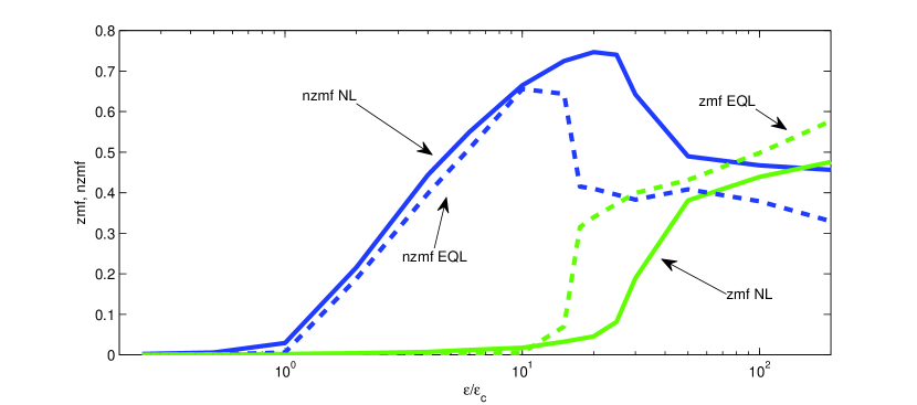
Figure 1: The zmf and nzmf indices defined in (5) and (6) respectively, as a function of energy input rate $\varepsilon/\varepsilon_{c}$ for the non-linear (NL) integrations and the ensemble quasi-linear (EQL) integrations (dashed line) with $N_{ens}=10$ ensemble members as described in section 6. The critical value $\varepsilon_{c}=8.4\cdot 10^{-6}$ is the energy input rate at which the S3T predicts structural instability of the homogeneous turbulent state. Zonal jets emerge for $\varepsilon>\varepsilon_{nl}$, with $\varepsilon_{nl}=15\varepsilon_{c}$. The parameters are $\beta=10$, $r=0.01$, $\nu=1.19\cdot 10^{-6}$ and the forcing is an isotropic ring in wavenumber space with radius $K_{f}=10$ and width $\Delta K_{f}=1$.

For $\varepsilon$ smaller than the critical value $\varepsilon_{c}$, the turbulent flow is homogeneous and remains translationally invariant in both directions and both indices are nearly zero. When $\varepsilon>\varepsilon_{c}$, non-zonal structures that have scales larger than the scale of the forcing form, as indicated by the increase in the nzmf index. The critical value is estimated from the point of rapid increase of the nzmf index to be $\varepsilon_{c}=8.4\cdot 10^{-6}$ (for the parameters chosen) but this value is also verified by the S3T stability analysis in section 4. The time averaged power spectrum shown in figure 2(a) for $\varepsilon=4\varepsilon_{c}$, is anisotropic with a pronounced peak at $(|k|,|l|)=(1,5)$. This peak corresponds to a structure with the corresponding scale that is evident in the vorticity field evolution. This is illustrated by the appearance of a structure with $(|k|,|l|)=(1,5)$ in the snapshot of the streamfunction field shown in figure 2(b). The Hovmöller diagram in which contours of $\psi(x,y=\pi/4,t)$ are plotted in figure 2(c) shows that this structure is coherent and propagates in the retrograde direction. The sloping dashed line in the diagram corresponds to the phase speed of the waves, which is found to be approximately the Rossby wave phase speed for $(k,l)=(1,5)$. We obtain an estimate of the phase coherence of this structure by calculating the ensemble mean of the wavenumber–frequency power spectrum of its vorticity field:

$$\zeta_{cor}(\omega,k,l)=\left<\left|\hat{\zeta}(k,l,\omega)\right|^{2}\right>,$$ (7)

where

$$\hat{\zeta}(k,l,\omega)=\int\sum_{x_{i}}\sum_{y_{i}}\zeta(x_{i},y_{i},t)\mathrm{e}^{-\mathrm{i}kx_{i}-\mathrm{i}ly_{i}-i\omega t}dt.$$ (8)

Traveling wave structures manifest as peaks of $\zeta_{cor}$ at specific frequencies with a half-width proportional to the time scale of their phase coherence. For example, for linear Rossby waves that are stochastically forced and damped with rate $1/r$:

$$\zeta_{cor}^{R}(\omega,k,l)\sim\frac{1}{\left[\omega-\beta k/(k^{2}+l^{2})\right]^{2}+r^{2}},$$ (9)

and the waves are phase correlated over the dissipation time scale (Galperin et al., 2010). We will consider the structures in the nonlinear simulation to be phase coherent when their coherence time exceeds $1/r$. Figure 2(d) shows the ensemble mean power spectrum $\zeta_{cor}(\omega,k,l)$ as obtained from the nonlinear simulations for two structures, along with the corresponding power spectrum $\zeta_{cor}^{R}$ of half-width $1/r$ for the same waves. The dominant $(|k|,|l|)=(1,5)$ structure is coherent over about four dissipation time scales, whereas the other less prominent structures (as for example the $(|k|,|l|)=(2,6)$ shown), are coherent over the dissipation time scale, as if stochastically forced. The $(|k|,|l|)=(1,5)$ structure dominates the flow (with 60% of the total energy concentrated in this structure) and remains coherent up to $\varepsilon/\varepsilon_{c}<15$. Therefore the increase in the nzmf index observed in figure 1 signifies the emergence of non-zonal coherent structures that break the translational symmetry of the turbulent state simultaneously in both the $x$ and $y$ direction.

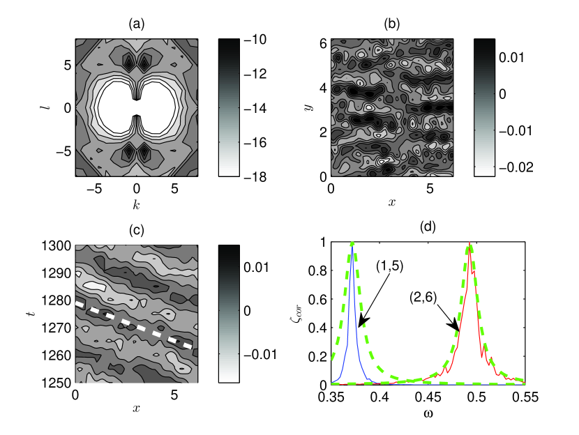
Figure 2: (a) Time averaged energy power spectra, $\log(\hat{E}(k,l))$, obtained from the non-linear (NL) simulation of (1) at $\varepsilon/\varepsilon_{c}=4$. The flow is dominated by a $(|k|,|l|)=(1,5)$ non-zonal coherent structure that is evident in the snapshot of the streamfunction $\psi(x,y,t)$ (panel b) and the Hovmöller diagram of $\psi(x,y=\pi/4,t)$ (panel c). The thick dashed line in (c) corresponds to the phase speed obtained from the eigenvalue relation (20). (d) The ensemble mean wavenumber–frequency power spectrum $\zeta_{cor}(\omega,k,l)$ as a function of frequency for $(k,l)=(1,5)$ and $(k,l)=(2,6)$. The corresponding spectrum $\zeta_{cor}^{R}$ for stochastically forced linear Rossby waves that remain phase coherent over $1/r$ is also shown (dashed lines). All correlation functions are normalized to one to facilitate comparison.

The rapid increase in the zmf index shown in figure 1 above $\varepsilon=15\varepsilon_{c}\equiv\varepsilon_{nl}$, indicates a second regime transition in the flow with the emergence of robust and coherent zonal jets. For $\varepsilon=3.3\varepsilon_{nl}$ (i.e. $\varepsilon/\varepsilon_{c}=50$) the spectrum, shown in figure 3(a), has significant power at the zonal structures with $(k,|l|)=(0,4)$. These peaks correspond to coherent zonal jets as illustrated by the Hovmöller diagram of the zonally averaged streamfunction shown in figure 3(b). However, there is significant power in non-zonal structures (in this case with wavenumbers $(|k|,|l|)=(1,4)$ and $(|k|,|l|)=(1,5)$), a characteristic that is also revealed by the high values of the nzmf index for large energy input rates. The Hovmöller diagram and the ensemble mean power spectrum $\zeta_{cor}(\omega,k,l)$ shown in figures 3(c) and 3(d), reveal that the non-zonal structures are propagating in the retrograde direction and remain coherent over at least a dissipation time scale, whereas the peaks of $\zeta_{cor}(\omega,k,l)$ at other structures have been significantly broadened by turbulence. The phase speed calculated from the diagram is different from the corresponding Rossby wave speed for both $(|k|,|l|)=(1,4)$ and $(|k|,|l|)=(1,5)$. At larger energy input rates the zonal jets have typically larger scales due to jet merging and coexist with energetically significant westward propagating non-zonal structures having an energy between $10-50\%$ of the jet energy and scales $(|k|,|l|)=(1,m)$, where $m$ is the number of jets in the channel. However the phase coherence of these waves is a decreasing function of $\varepsilon$.

Similar Rossby-like, westward propagating coherent structures were also reported recently in numerical simulations of the barotropic vorticity equation on the sphere (Sukariansky et al., 2008; Galperin et al., 2010). In agreement with the results presented in this work these large scale waves contain a significant amount of energy. In the regime in which zonal jets are absent or weak these waves were found to follow the Rossby wave dispersion. In the regime in which strong zonal jets dominate the flow (called the zonostrophic regime by these authors), the waves propagate with markedly different phase speeds. These waves were therefore classified as linear Rossby waves in the former and as satellite modes (Danilov & Gurarie, 2004) or zonons (Sukariansky et al., 2008) in the latter regime.

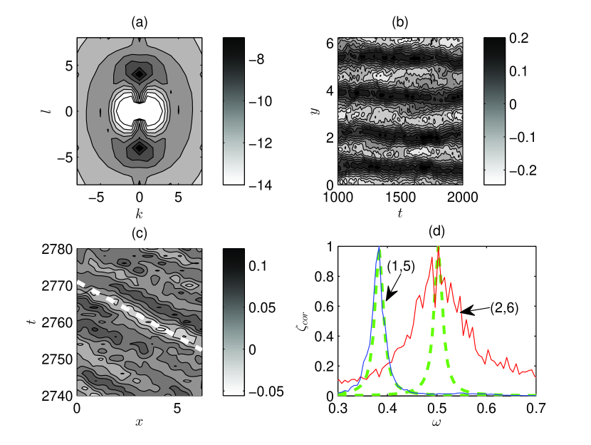
Figure 3: (a) Time averaged energy power spectra, $\log(\hat{E}(k,l))$, obtained from the non-linear simulation of (1) at $\varepsilon/\varepsilon_{c}=50$. The flow is dominated by a $(k,|l|)=(0,4)$ zonal jet that is evident in the Hovmöller diagram of the $x$-averaged $\overline{\psi(x,y,t)}$ (panel b). (c) Hovmöller diagram of $\psi(x,y=\pi/4,t)$ showing the presence of westward propagating structures. The thick dashed line corresponds to the phase speed obtained from (20). (d) The ensemble mean wavenumber–frequency power spectrum $\zeta_{cor}(\omega,k,l)$ as a function of frequency for $(k,l)=(1,5)$ and $(k,l)=(2,6)$. The corresponding spectrum $\zeta_{cor}^{R}$ for stochastically forced linear Rossby waves is also shown (dashed lines). All correlation functions are normalized to one to facilitate comparison.

We will show next that the emergence and characteristics of both the zonal and the non-zonal coherent structures can be accurately predicted by considering the stability of a particular second order closure of the turbulent dynamics. This second order closure results in a non-equilibrium statistical theory, called Stochastic Structural Stability Theory (S3T) or Second Order Cumulant Expansion theory (CE2) (Farrell & Ioannou, 2003, 2007; Marston et al., 2008; Bakas & Ioannou, 2011; Srinivasan & Young, 2012; Marston, 2012), that addresses the emergence of structure in planetary turbulence.

3 Formulation of Stochastic Structural Stability Theory

S3T describes the statistical dynamics of the first two equal time cumulants of (1). The first cumulant is the ensemble mean of the vorticity $Z(\mathbf{x},t)\equiv\left<\zeta\right>$. The second cumulant $C(\mathbf{x}_{1},\mathbf{x}_{2},t)\equiv\left<\zeta_{1}^{\prime}\zeta_{2}^{\prime}\right>$, is the two point correlation function of the vorticity deviation from the mean $\zeta_{i}^{\prime}\equiv\zeta_{i}-Z_{i}$. We use the shorthand $\zeta_{i}=\zeta(\mathbf{x}_{i},t)$, with $i=1,~{}2$ to refer to the value of the relative vorticity at the specific point $\mathbf{x}_{i}=(x_{i},y_{i})$. In most earlier studies of S3T, the ensemble average was assumed to represent a zonal average. With this interpretation of the ensemble average, the non-zonal structures are treated as incoherent motions and the theory can only address the emergence of zonal jets. In order to address the emergence of coherent non-zonal structures in turbulence, we adopt in this work the more general interpretation that the ensemble average is a Reynolds average over the fast turbulent motions that typically have time scales in this case $\tau_{eddy}\ll 1/r$. The averaging time scale is taken to be several eddy decorrelation scales but also smaller than $1/r$ and smaller than the period of the propagating structures (for a periodic box the lowest period is of order $1/\beta$) in order to retain the slow evolution of the coherent structures. This interpretation of the S3T has been adopted recently in studies of non-zonal blocking patterns in baroclinic two-layer turbulence by Bernstein (2009) and Bernstein & Farrell (2010). With this definition of the ensemble mean, we seek to obtain the statistical dynamics of the interaction of the coarse-grained ensemble average field, which can be zonal or non-zonal coherent structures represented by their vorticity $Z$, with the fine-grained incoherent field represented by the vorticity second cumulant $C$.

The equations governing the evolution of the first two cumulants are obtained as follows. Under the decomposition of vorticity into an ensemble mean and a deviation from the mean, (1) is split into two equations governing the evolution of the eddy (deviation from the mean) vorticity $\zeta^{\prime}$ and the vorticity of the coherent structures $Z$:

$$\left(\partial_{t}+\boldsymbol{U}\cdot\nabla\right)\zeta^{\prime}+(\beta+\partial_{y}Z)v^{\prime}+u^{\prime}\partial_{x}Z=-r\zeta^{\prime}-\nu\Delta^{2}\zeta^{\prime}+\underbrace{f^{e}+f^{nl}}_{f},$$ (10)

$$\left(\partial_{t}+\boldsymbol{U}\cdot\nabla\right)Z+\beta V=-\nabla\cdot\left<\boldsymbol{u}^{\prime}\zeta^{\prime}\right>-rZ-\nu\Delta^{2}Z,$$ (11)

where $\boldsymbol{u}^{\prime}=[u^{\prime},v^{\prime}]=[-\partial_{y}\psi^{\prime},\partial_{x}\psi^{\prime}]$ and $\boldsymbol{U}=[U,V]=[-\partial_{y}\Psi,\partial_{x}\Psi]$ are the non-divergent eddy and ensemble mean velocity fields,

$$f^{nl}=\left<\boldsymbol{u}^{\prime}\cdot\nabla\zeta^{\prime}\right>-\boldsymbol{u}^{\prime}\cdot\nabla\zeta^{\prime},$$ (12)

is the forcing term from the non-linear interactions among the turbulent eddies and $f=f^{e}+f^{nl}$ represents the total eddy forcing. The ensemble average vorticity fluxes $\left<\mathbf{u}^{\prime}\zeta^{\prime}\right>$ can be expressed in terms of the second cumulant of vorticity as:

$$\left<\mathbf{u}^{\prime}\zeta^{\prime}\right>=\left[\left<u_{1}^{\prime}\zeta_{2}^{\prime}\right>_{\mathbf{x}_{1}=\mathbf{x}_{2}},\left<v_{1}^{\prime}\zeta_{2}^{\prime}\right>_{\mathbf{x}_{1}=\mathbf{x}_{2}}\right]=\left[-\left(\partial_{y_{1}}\Delta_{1}^{-1}C\right)_{\mathbf{x}_{1}=\mathbf{x}_{2}},\left(\partial_{x_{1}}\Delta_{1}^{-1}C\right)_{\mathbf{x}_{1}=\mathbf{x}_{2}}\right],$$ (13)

where $\Delta^{-1}$ is the integral operator that inverts vorticity into the streamfunction field ($\psi=\Delta^{-1}\zeta$). The subscripts in the operators in (13) denote the variable $\mathbf{x}_{i}$ on which the operators act. For example $\partial_{x_{i}}$ denotes differentiation with respect the variable $x_{i}$ ($i=1,2$), while the integral operators $\Delta_{i}^{-1}$ invert the vorticity covariance with respect to variables $\mathbf{x}_{i}$ so that the streamfunction covariance is $S(\mathbf{x}_{1},\mathbf{x}_{2})=\Delta^{-1}_{1}\Delta^{-1}_{2}C$. The subscript $\mathbf{x}_{1}=\mathbf{x}_{2}$ means that the expression in parenthesis is calculated at the same point. As a result, the first cumulant evolves as:

$$\partial_{t}Z+UZ_{x}+V(\beta+Z_{y})=\partial_{x}\left(\partial_{y_{1}}\Delta_{1}^{-1}C\right)_{\mathbf{x}_{1}=\mathbf{x}_{2}}-\partial_{y}\left(\partial_{x_{1}}\Delta_{1}^{-1}C\right)_{\mathbf{x}_{1}=\mathbf{x}_{2}}-rZ-\nu\Delta^{2}Z.$$ (14)

Multiplying (10) for $\partial_{t}\zeta_{1}^{\prime}$ by $\zeta_{2}^{\prime}$ and (10) for $\partial_{t}\zeta_{2}^{\prime}$ by $\zeta_{1}^{\prime}$, adding the two equations and taking the ensemble average yields:

$$\partial_{t}C=(A_{1}+A_{2})C+\left<f_{1}\zeta_{2}^{\prime}+f_{2}\zeta_{1}^{\prime}\right>,$$ (15)

where

$$A_{i}=-U_{i}\partial_{x_{i}}-V_{i}\partial_{y_{i}}-(\beta+\partial_{y_{i}}Z)\partial_{x_{i}}\Delta_{i}^{-1}+\partial_{x_{i}}Z\partial_{y_{i}}\Delta_{i}^{-1}-r-\nu\Delta_{i}^{2},$$ (16)

governs the dynamics of linear perturbations about the instantaneous mean flow $\boldsymbol{U}$,

$$\left<f_{1}\zeta_{2}^{\prime}+f_{2}\zeta_{1}^{\prime}\right> = \left<f_{1}^{e}\zeta_{2}^{\prime}+f_{2}^{e}\zeta_{1}^{\prime}\right>+\left<f_{1}^{nl}\zeta_{2}^{\prime}+f_{2}^{nl}\zeta_{1}^{\prime}\right>$$ (17)

$$= \left<f_{1}^{e}\zeta_{2}^{\prime}+f_{2}^{e}\zeta_{1}^{\prime}\right>+$$

$$+ \left[\left(\partial_{y_{1}x_{3}}^{2}-\partial_{x_{1}y_{3}}^{2}\right)\Delta_{2}^{-1}\Gamma\right]_{\mathbf{x}_{1}=\mathbf{x}_{3}}+\left[\left(\partial_{y_{2}x_{3}}^{2}-\partial_{x_{2}y_{3}}^{2}\right)\Delta_{2}^{-1}\Gamma\right]_{\mathbf{x}_{2}=\mathbf{x}_{3}},$$

and $\Gamma\equiv\left<\zeta_{1}^{\prime}\zeta_{2}^{\prime}\zeta_{3}^{\prime}\right>$ is the third cumulant. The first term on the right hand side of (17) is the correlation of the external forcing $f^{e}$ with vorticity, while the other two terms involve the third cumulant that describes the eddy-eddy interactions. Previous studies addressing the interaction of turbulent eddies with zonal jets in baroclinic turbulence, as well as the interaction of coherent vortices with small scale turbulence, have shown that several important features of the coherent flow as well as accurate eddy statistics are obtained by either neglecting or suitably parameterizing the eddy-eddy non-linearity $f^{nl}$ as stochastic forcing and enhanced dissipation (Farrell & Ioannou, 1993a; DelSole & Farrell, 1996; Dubrulle & Nazarenko, 1997; Laval et al., 2000; DelSole, 2004; O’Gorman & Schneider, 2007; Marston et al., 2008). This is equivalent to setting the third cumulant to zero, or parameterizing the last two terms in (17) as a given correlation function. We note that the distinction between these two parameterizations is semantic for barotropic turbulence sustained by stochastic forcing. However, if turbulence is self-maintained without any external stochastic forcing, as for example is the case in baroclinic flows, and the third cumulant is altogether neglected then the covariance in (15) is unforced and will evolve to the low rank structure of the Lyapunov vector of the generally time dependent $A$ operator. As a result, it will fail to accurately represent the second order statistics of the turbulent flow (Marston et al., 2008). The presence of the parameterization of the nonlinear eddy-eddy scattering as noise in this case, is therefore important because it keeps the structure of the second order cumulant full rank and in accordance to the amplification properties of the non-normal $A$ operator. In this work we will neglect the third-order cumulants and show that the S3T theory with this approximation can accurately predict the emergence of large scale structures in the flow. We therefore assume that $f$ is the delta correlated external forcing, $f^{e}$, with $\left<f_{1}\zeta_{2}^{\prime}+f_{2}\zeta_{1}^{\prime}\right>=\left<f_{1}f_{2}\right>=\Xi$. With this approximation the second order statistics evolve according to:

$$\partial_{t}C=(A_{1}+A_{2})C+\Xi.$$ (18)

Equations (14) and (18) form a closed deterministic system that governs the joint evolution of the coherent flow field and of the second order turbulent eddy statistics. This second order closure is the basis of Stochastic Structural Stability Theory (Farrell & Ioannou, 2003). The S3T system can have fixed points, limit cycles or chaotic attractors. Examples of the attractor of this system can be found in the S3T description of the organization of geophysical and plasma turbulence into zonal jets (Farrell & Ioannou, 2003, 2008, 2009b), as well as in the S3T description of blocking patterns in the atmosphere (Bernstein & Farrell, 2010). The fixed points $Z^{E}$ and $C^{E}$, if they exist, define statistical equilibria of the coherent structures with vorticity, $Z^{E}$, in the presence of an eddy field with covariance, $C^{E}$. The structural stability of these turbulent equilibria that can be investigated in S3T, addresses the parameters in the physical system which can lead to abrupt reorganization of the turbulent flow. Specifically, when an equilibrium of the S3T equations becomes unstable as a physical parameter changes, the turbulent flow bifurcates to a different attractor. In this work, we show that coherent structures emerge as unstable modes of the S3T system and equilibrate at finite amplitude. The predictions of the S3T system regarding the emergence and characteristics of the coherent structures are then compared to the non-linear simulations.

4 S3T instability and emergence of finite amplitude large scale structure

The homogeneous equilibrium with no mean flow

$$Z^{E}=0,~{}~{}C^{E}={\Xi\over 2r},$$ (19)

is a fixed point of the S3T system (14) and (18) in the absence of hyperdiffusion (cf. Appendix B). The stability of this homogeneous equilibrium, can be addressed by performing eigenanalysis of the S3T system linearized about the equilibrium. Because of the absence of coherent mean flow and the homogeneity of $C^{E}$ we can seek eigensolutions in the modal form $\delta Z=Z_{nm}\mathrm{e}^{\mathrm{i}nx+\mathrm{i}my}\mathrm{e}^{\sigma t}$ and $\delta C=C_{nm}(\tilde{x},\tilde{y})\mathrm{e}^{\mathrm{i}n\overline{x}+\mathrm{i}m\overline{y}}\mathrm{e}^{\sigma t}$, where $\tilde{x}=x_{1}-x_{2}$, $\overline{x}=(x_{1}+x_{2})/2$, $\tilde{y}=y_{1}-y_{2}$, $\overline{y}=(y_{1}+y_{2})/2$, $n$ and $m$ are the $x$ and $y$ wavenumbers of the eigenfunction and $\sigma=\sigma_{r}+\mathrm{i}\sigma_{i}$ is the eigenvalue with $\sigma_{r}=\mbox{Re}(\sigma)$, $\sigma_{i}=\mbox{Im}(\sigma)$ being the growth rate and frequency of the mode respectively. The eigenvalue $\sigma$ satisfies the equation:

$$\int_{-\infty}^{\infty}\int_{-\infty}^{\infty}\frac{(mk-nl)\left[nm(k_{+}^{2}-l_{+}^{2})+(m^{2}-n^{2})k_{+}l_{+}\right](1-N^{2}/K^{2})\hat{\Xi}(k,l)}{2\mathrm{i}\beta k_{+}(k_{+}n+l_{+}m)-\mathrm{i}n\beta\left(K^{2}+K_{s}^{2}\right)/2+(\sigma+2r)K^{2}K_{s}^{2}}\mathrm{d}k\mathrm{d}l$$ (20)

$$= 2r\pi(\sigma+r)N^{2}-2r\mathrm{i}\pi n\beta,$$

where

$$\hat{\Xi}(k,l)=\frac{1}{2\pi}\int_{-\infty}^{\infty}\int_{-\infty}^{\infty}\Xi(\tilde{x},\tilde{y})\mathrm{e}^{-\mathrm{i}k\tilde{x}-\mathrm{i}l\tilde{y}}\mathrm{d}\tilde{x}\mathrm{d}\tilde{y}~{},$$ (21)

is the Fourier transform of the forcing covariance, $K^{2}=k^{2}+l^{2}$, $K_{s}^{2}=(k+n)^{2}+(l+m)^{2}$, $N^{2}=n^{2}+m^{2}$, $k_{+}=k+n/2$ and $l_{+}=l+m/2$ (cf. Appendix B). For zonally homogeneous perturbations with $n=0$, (20) reduces to the eigenvalue relation derived by Srinivasan & Young (2012) for the emergence of jets in a barotropic $\beta$-plane. Eigenvalue relation (20) was derived for a flow that extends to infinity. For the periodic channel considered in the non-linear simulations, the corresponding eigenvalue relation is readily obtained by substituting the integrals in (20) and (21) with summation over integer values of $k$ and $l$ (Bakas & Ioannou, 2013a). We non-dimensionalize the eigenvalue relation using the dissipation time scale $1/r$ and a typical forcing length scale $L_{f}$ and rewrite (20) in the general form:

$$\tilde{\sigma}_{(\tilde{n},\tilde{m})}=g(\tilde{\beta},\tilde{\varepsilon}).$$ (22)

For a given spectral distribution of the forcing, (22) gives the eigenvalue $\tilde{\sigma}=\sigma/r$ for each wavenumbers $(\tilde{n},\tilde{m})=L_{f}(n,m)$ as a function of the planetary vorticity gradient $\tilde{\beta}=\beta L_{f}/r$ and the energy injection rate $\tilde{\varepsilon}=\varepsilon/(r^{3}L_{f}^{2})$.

We consider the case of a ring forcing that injects energy at rate $\varepsilon$ at the total wavenumber $K_{f}$:

$$\hat{\Xi}(k,l)=2\varepsilon K_{f}\delta(\sqrt{k^{2}+l^{2}}-K_{f}),$$ (23)

which is an idealization of the forcing (4) used in the non-linear simulations. We then obtain the eigenvalues $\tilde{\sigma}$ for an infinite domain by numerically solving (22). For small values of the energy input rate, the growth rate $\tilde{\sigma}_{r}$ is negative for all $(\tilde{n},\tilde{m})$ and the homogeneous equilibrium is stable. At a critical $\tilde{\varepsilon}_{c}$ the homogeneous flow becomes S3T unstable, symmetry breaking occurs and exponentially growing coherent structures emerge. The critical value, $\tilde{\varepsilon}_{c}$, is calculated by first determining the energy input rate $\tilde{\varepsilon}_{t}(\tilde{n},\tilde{m})$ that renders wavenumbers $(\tilde{n},\tilde{m})$ neutral $\left(\tilde{\sigma}_{r(\tilde{n},\tilde{m})}=0\right)$, and then by finding the minimum energy input rate over all wavenumbers: $\tilde{\varepsilon}_{c}=\mbox{min}_{(\tilde{n},\tilde{m})}\tilde{\varepsilon}_{t}$. The critical energy input rate $\tilde{\varepsilon}_{c}$ as a function of $\tilde{\beta}$ is shown in figure 4. The absolute minimum energy input rate required is $\tilde{\varepsilon}_{c}=67$ and occurs at $\tilde{\beta}_{min}=3.5$. For $\tilde{\beta}\leq\tilde{\beta}_{min}$, the structures that first become marginally stable are zonal jets (with $n=0$). The critical input rate increases as $\tilde{\varepsilon}_{c}\sim\tilde{\beta}^{-2}$ for $\tilde{\beta}\rightarrow 0$ (in agreement with the findings of Srinivasan & Young (2012)) and the homogeneous equilibrium is structurally stable for all excitation amplitudes when $\tilde{\beta}=0$. The structural stability for $\tilde{\beta}=0$ is an artifact of the assumed isotropy of the excitation and in the presence of anisotropy the critical input rate, $\tilde{\varepsilon}_{c}$, saturates to a finite value as $\tilde{\beta}\rightarrow 0$ (Bakas & Ioannou, 2011, 2013b). For $\tilde{\beta}>\tilde{\beta}_{min}$, the marginally stable structures are non-zonal and $\tilde{\varepsilon}_{c}$ grows as $\tilde{\varepsilon}_{c}\sim\tilde{\beta}^{1/2}$ for $\tilde{\beta}\rightarrow\infty$. Since the critical forcing for the emergence of zonal jets (also shown in figure 4), increases as $\tilde{\varepsilon}_{c}\sim\tilde{\beta}^{2}$ for $\tilde{\beta}\rightarrow\infty$ (Srinivasan & Young, 2012), for large values of $\tilde{\beta}$ non-zonal structures first emerge and only at significantly higher $\tilde{\varepsilon}$ zonal jets are expected to appear. Investigation of these results with other forcing distributions revealed that these results are independent of the isotropy of the forcing. Contours of the maximum growth rate of the S3T instability, $\tilde{\sigma}_{max}=\mbox{max}_{(\tilde{n},\tilde{m})}\tilde{\sigma}_{r}$ are also shown in figure 4 as a function of $(\tilde{\varepsilon},\tilde{\beta})$. For a given $\tilde{\beta}$, the maximum growth rate increases monotonically with larger energy input rates, while for a given level of excitation $\tilde{\varepsilon}_{m}$ the maximum growth rate occurs for a finite $\tilde{\beta}_{m}$ that satisfies roughly $\tilde{\varepsilon}_{m}\sim 30\tilde{\beta}_{m}^{2}$ (represented by the thick dotted line in the figure).

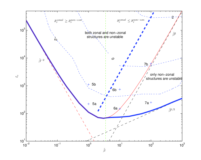
Figure 4: The critical energy input rate $\tilde{\varepsilon}_{c}$ for structural instability (thick solid line) and the critical energy input rate for structural instability of zonal jets (solid line) as a function of $\tilde{\beta}$. The behavior of these critical values for large and small $\tilde{\beta}$ is indicated with the dashed asymptotes $\tilde{\varepsilon}=23\tilde{\beta}^{-2}$ for $\tilde{\beta}\ll 1$, $\tilde{\varepsilon}=11\tilde{\beta}^{1/2}$ and $\tilde{\varepsilon}=0.5\tilde{\beta}^{2}$ for the emergence of non-zonal and zonal structures respectively for $\tilde{\beta}\gg 1$. Above the thick (thin) line non-zonal (zonal) coherent structures emerge. The thin dotted vertical line $\tilde{\beta}=\tilde{\beta}_{min}$ separates the unstable region: for $\tilde{\beta}<\tilde{\beta}_{min}$ the zonal structures grow the most, whereas for $\tilde{\beta}>\tilde{\beta}_{min}$ the non-zonal structures grow the most. Also shown are the contours (thick dashed lines) of the maximum growth rate $\tilde{\sigma}_{max}$ (with contour values corresponding to $\log(\tilde{\sigma}_{max})$). The thick dotted line $\tilde{\varepsilon}=30\tilde{\beta}^{2}$ is the locus of the points on which the maximum $\tilde{\sigma}_{r}$ occurs for each $\tilde{\varepsilon}$. The crosses indicate the $\tilde{\varepsilon}$ and $\tilde{\beta}$ values for which the dispersion relation of the unstable modes is shown in figures 5-7.

For $\tilde{\varepsilon}>\tilde{\varepsilon}_{c}$ there is a number of structures that grows exponentially. It is shown in Appendix B that for the isotropic forcing considered and for $n\neq 0$, the eigenvalues satisfy the relations:

$$\tilde{\sigma}_{(-\tilde{n},\tilde{m})}=\tilde{\sigma}_{(\tilde{n},\tilde{m})}^{*},\mbox{~{}and~{}}\tilde{\sigma}_{(\tilde{n},-\tilde{m})}=\tilde{\sigma}_{(\tilde{n},\tilde{m})},$$ (24)

implying that the growth rates depend on $|\tilde{n}|$ and $|\tilde{m}|$. As a result, the plane wave $\delta Z=\cos(nx+my)$ and an array of localized vortices $\delta Z=\cos(nx)\cos(my)$, have the same growth rate, despite their different structure.

We first consider the case $\tilde{\beta}=1$, $\tilde{\varepsilon}=2\tilde{\varepsilon}_{c}$, corresponding to the point marked as 5a in the $(\tilde{\varepsilon},\tilde{\beta})$ regime diagram shown in figure 4. The growth rate of the maximally growing eigenvalue, $\tilde{\sigma}_{r}$, and its associated frequency of the mode, $\tilde{\sigma}_{i}$, are plotted in figure 5a as a function of $|\tilde{n}|$ and $|\tilde{m}|$. We observe that the region in wavenumber space defined roughly by $0<|\tilde{n}|<1/2,\mbox{~{}and~{}}1/2<|\tilde{m}|<1$ is unstable, with the maximum growth rate occurring for zonal structures ($\tilde{n}=0$) with $|\tilde{m}|\simeq 0.8$. The frequency of the unstable modes is in general non-negative ($\tilde{\sigma}_{i}\geq 0$) and is equal to zero only for zonal jet perturbations ($\tilde{n}=0$). Using the symmetries (24), this implies that real unstable mean flow perturbations $\delta Z$ propagate in the retrograde direction if $\tilde{n}\neq 0$ and are stationary when $\tilde{n}=0$. As $\tilde{\varepsilon}$ increases the instability region expands roughly covering the sector $1/2<|\tilde{N}|<1$ and a second instability branch with smaller growth rates appears for $|\tilde{N}|>1$. This is illustrated in figure 5b showing the growth rate for $\tilde{\varepsilon}=10\tilde{\varepsilon}_{c}$ (marked as 5b in figure 4). Note also that for both values of the energy input rate, the zonal structures have a larger growth rate than the non-zonal structures, a result that holds for any $\tilde{\varepsilon}$ when $\tilde{\beta}<\tilde{\beta}_{min}$.

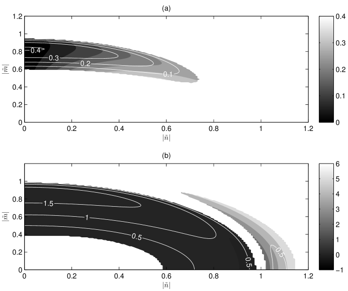
Figure 5: Dispersion relation of the unstable modes for $\tilde{\beta}=1$. The energy input rate is (a) $\tilde{\varepsilon}=2\tilde{\varepsilon}_{c}$ and (b) $\tilde{\varepsilon}=10\tilde{\varepsilon}_{c}$. The contours show the growth rate $\tilde{\sigma}_{r}$ and the shading shows the frequency $\tilde{\sigma}_{i}$ of the unstable modes.

For $\tilde{\beta}>\tilde{\beta}_{min}$ the non-zonal structures have always larger growth rate. This is illustrated in figures 6 and 7, showing the growth rates and frequencies of the unstable modes for $\tilde{\beta}=10$ and $\tilde{\beta}=100$ respectively. For larger $\tilde{\beta}$ values there is tendency for the frequency of the unstable modes to conform to the corresponding Rossby wave frequency

$$\tilde{\sigma}_{R}=\frac{\tilde{\beta}\tilde{n}}{\tilde{n}^{2}+\tilde{m}^{2}}~{},$$ (25)

a tendency that does not occur for smaller $\tilde{\beta}$. A comparison between the frequency of the unstable mode and the Rossby wave frequency is shown in figures 7(c),(d) in a plot of $\tilde{\sigma}_{i}/\tilde{\sigma}_{R}$. For slightly supercritical $\tilde{\varepsilon}$, the ratio is close to one and the unstable modes satisfy the Rossby wave dispersion relation. At higher supercriticalities though, $\tilde{\sigma}_{i}$ departs from the Rossby wave frequency (by as much as $40\%$ for the case of $\tilde{\varepsilon}=50\tilde{\varepsilon}_{c}$ shown in figure 7(d)).

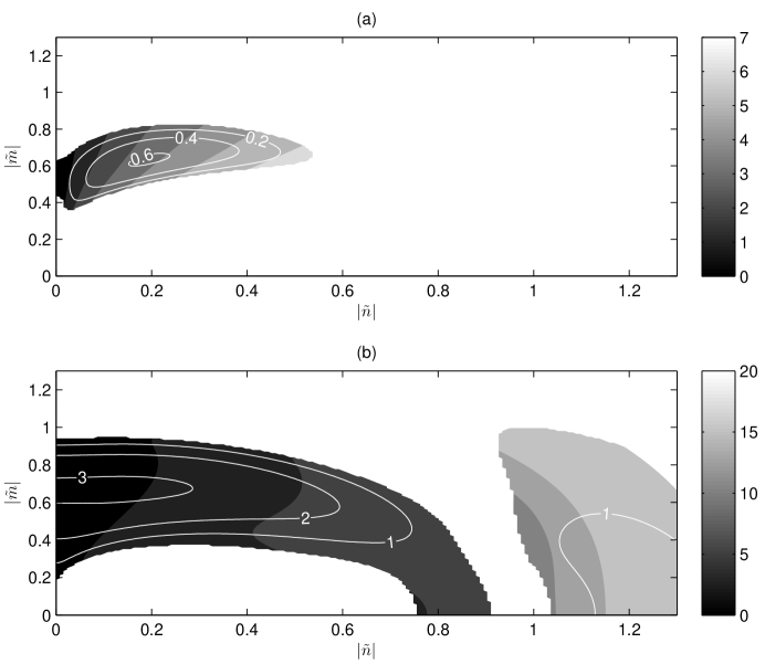
Figure 6: The same as in figure 5, but for $\tilde{\beta}=10$.

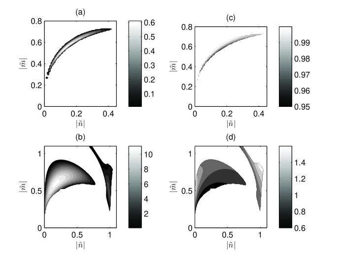
Figure 7: Dispersion relation of the unstable modes for $\tilde{\beta}=100$. Growth rate $\tilde{\sigma}_{r}$ as a function of wavenumbers $(\tilde{n},\tilde{m})$ at (a) $\tilde{\varepsilon}=2\tilde{\varepsilon}_{c}$ and (b) $\tilde{\varepsilon}=50\tilde{\varepsilon}_{c}$. Only positive values are shown. Ratio of the frequency of the unstable modes $\tilde{\sigma}_{i}$ over the corresponding frequency of a Rossby wave with the same wavenumbers $\tilde{\sigma}_{R}$ at (c) $\tilde{\varepsilon}=2\tilde{\varepsilon}_{c}$ and (d) $\tilde{\varepsilon}=50\tilde{\varepsilon}_{c}$. Values of one denote an exact match with the Rossby wave phase speed.

5 Equilibration of the S3T instabilities

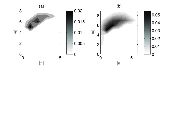
Figure 8: The growth rate, $\sigma_{r}$ as a function of the wavenumbers $|n|$, $|m|$ of the coherent structures at (a) $\varepsilon/\varepsilon_{c}=4$ and (b) $\varepsilon/\varepsilon_{c}=10$ (only positive values of $\sigma_{r}$ are shown). The growth rates are calculated for structures in the doubly periodic channel considered in the non-linear simulations and in the presence of hyper-diffusion with coefficient $\nu=1.19\cdot 10^{-6}$.

We now investigate the equilibration of the instabilities by the discretized S3T system (14), (18) in a doubly periodic channel of size $2\pi\times 2\pi$. We consider the parameter values chosen in the non-linear simulations discussed in section 2 ($\beta=10$, $r=0.01$, $\nu=1.19\cdot 10^{-6}$, $K_{f}=10$ and $\Delta K_{f}=1$). For these parameters, $\tilde{\beta}=100$ and therefore the integration is in the parameter region of figure 4 in which the non-zonal structures are more unstable than the zonal jets. We first consider the energy input rate $\tilde{\varepsilon}=4\tilde{\varepsilon}_{c}$ which corresponds to the first case presented in section 2 . The growth rates of the coherent structures for integer values of the wavenumbers, $n$ and $m$ are calculated from the discrete version of equation (20), because of the $2\pi$ periodicity of the channel, with the addition of a hyperdiffusive dissipation term in equation (20). The resulting growth rates for this energy input rate are shown in figure 8(a). For these parameters the zonal jet perturbations are stable and are not expected to emerge, while a large number of non-zonal modes are unstable with the perturbation $(n,m)=(1,5)$ growing the most. At $t=0$, we introduce a small random perturbation, whose streamfunction is shown in figure 9(a). After about $t=40/\sigma_{(1,5)}$, where $\sigma_{(1,5)}$ is the growth rate of $(n,m)=(1,5)$, a checkerboard perturbation of the form $Z=\cos(x)\cos(5y)$ dominates the large scale flow. The evolution of the energy of the large scale flow that is shown in figure 9(b) increases rapidly and eventually saturates after about $t=150/\sigma_{(1,5)}$. At this point the large scale flow gets attracted to a traveling wave finite amplitude equilibrium structure close in form to the harmonic $Z=\cos(x)\cos(5y)$ (cf. figure 9(c)), drifting westward. The Hovmöller diagram of $\psi(x,y=\pi/4,t)$, shown in 9(d), illustrates that the phase speed of the traveling wave is approximately equal to the phase speed of the unstable $(n,m)=(1,5)$ eigenmode that is also indicated in the figure.

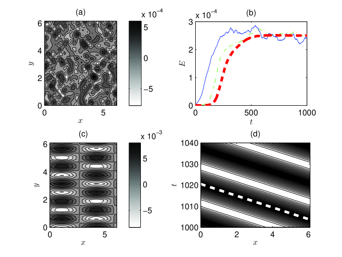
Figure 9: Equilibration of the S3T instabilities. (a) Streamfunction of the initial perturbation. (b) Energy evolution of the initial perturbation shown in panel (a) as obtained from the integration of the S3T equations (14) and (18) (dashed line) and from the integration of the ensemble quasi-linear (EQL) system (10)-(11) with $N_{ens}=10$ (solid line) and $N_{ens}=100$ (dash-dotted line) ensemble members that is discussed in section 6. (c) Snapshot of the streamfunction $\Psi_{eq}$ of the traveling wave structure and (d) Hovmöller diagram of $\Psi_{eq}(x,y=\pi/4,t)$ for the finite equilibrated traveling wave. The thick dashed line shows the phase speed obtained from the stability equation (20). The energy input rate is $\tilde{\varepsilon}=4\varepsilon_{c}$ and $\tilde{\beta}=100$.

Consider now the energy input rate $\tilde{\varepsilon}=10\tilde{\varepsilon}_{c}$ for which the growth rates are shown in figure 8(b). While the maximum growth rate still occurs for the $(|n|,|m|)=(1,5)$ non-zonal structure, zonal jet perturbations are unstable as well. In previous studies of S3T dynamics restricted to the interaction between zonal flows and turbulence, these initially S3T unstable jet structures were found to equilibrate at finite amplitude. However, in the context of the generalized S3T analysis in this work that takes into account the dynamics of the interaction between coherent non-zonal structures and jets, we find that these S3T jet equilibria can be saddles: stable to zonal jet perturbations but unstable to non-zonal perturbations. To show this, we consider the evolution of a small zonal jet perturbation $\delta Z=0.001\cos(5y)$ that is shown in figure 10. The initial perturbation grows exponentially and its energy saturates at about $t=500$ (a snapshot of the streamfunction at this time is shown at the left inset in figure 10). But soon after, non-zonal undulations appear and start to grow and the flow transitions to the stable $Z=\cos(x)\cos(5y)$ traveling wave state that is also shown in figure 10. As a result, the finite equilibrium zonal jet structure is S3T unstable to coherent non-zonal perturbations and is not expected to appear in non-linear simulations despite the fact that the zero flow equilibrium is unstable to zonal jet perturbations. We will elaborate more on this issue in the next section.

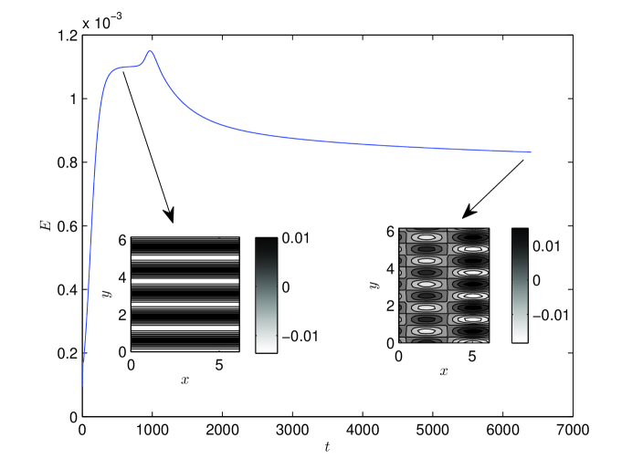
Figure 10: Energy evolution of an initial jet perturbation $\delta Z=0.001\cos(5y)$ for $\tilde{\varepsilon}=10\varepsilon_{c}$ and $\tilde{\beta}=100$. The insets show a snapshot of the mean flow streamfunction at $t=500$ (left) and the streamfunction of the equilibrated structure at $t=6500$ (right).

Finally, consider the case $\varepsilon=30\varepsilon_{c}$. At this energy input rate, the fast growing non-zonal perturbations cannot equilibrate, as the finite amplitude non-zonal traveling wave equilibria become S3T unstable. This is illustrated in figure 11 showing the evolution of a small non-zonal perturbation $\delta Z=0.01\cos(x)\cos(5y)$. After the saturation of the initial instability at about $t=200$, the flow transitions slowly from the traveling wave $Z=\cos(x)\cos(5y)$ state shown at the left inset in figure 11 to the jet equilibrium state shown at the right inset in figure 11. Note however, that the jet equilibrium structure is not zonally symmetric. This is a new type of S3T equilibrium: it is a mix between a zonal jet and a non-zonal traveling wave and actually S3T analysis reveals multiple mixed state equilibria. This is clearly illustrated in figure 12 showing the structure of a different equilibrium state for the same parameters. The equilibrium structure consists of a large amplitude zonally symmetric jet with small amplitude non-zonal propagating vortices embedded in it. These vortices that are shown in figure 12(b) to have approximately the compact support structure $\Psi=\cos(2x)\cos(6y)$ propagate westward as shown in the Hovmöller diagram in figure 12(c).

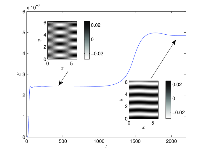
Figure 11: Energy evolution of the initial non-zonal perturbation $\delta Z=0.01\cos(x)\cos(5y)$ for $\tilde{\varepsilon}=30\varepsilon_{c}$ and $\tilde{\beta}=100$. The insets show a snapshot of the mean flow streamfunction at $t=200$ (left) and the streamfunction of the equilibrated structure at $t=2200$ (right).

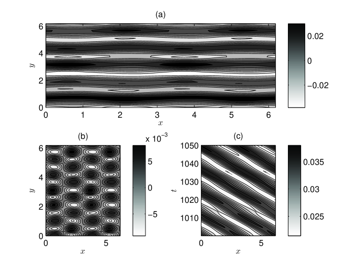
Figure 12: Mixed zonal jet-traveling wave S3T equilibrium for $\tilde{\varepsilon}=30\varepsilon_{c}$ and $\tilde{\beta}=100$. (a) Snapshot of the streamfunction $\Psi_{eq}$ of the equilibrium state. (b) Contour plot of the non-zonal component $\Psi_{eq}-\overline{\Psi_{eq}}$ of the equilibrium structure, where the overline denotes a zonal average. (c) Hovmöller diagram of $\Psi_{eq}(x,y=\pi/4,t)$ for the equilibrated structure. In this mixed S3T equilibrium zonal jets coexist with vortices reminiscent of the coherent structures observed in Jupiter.

6 Comparison to non-linear simulations

Within the context of the second order cumulant closure, the S3T formulation allows the identification of statistical turbulent equilibria. These S3T equilibria and their stability properties are manifest even in single realizations of the turbulent system. For example, previous studies using S3T obtained zonal jet equilibria in barotropic, shallow water and baroclinic flows in close correspondence with observed jets in planetary flows (Farrell & Ioannou, 2007, 2008, 2009c, 2009a). In addition, previous studies of S3T dynamics restricted to the interaction between zonal flows and turbulence in a $\beta$-plane channel showed that when the energy input rate is such that the zero mean flow equilibrium is unstable, zonal jets also appear in the non-linear simulations with the structure (scale and amplitude) predicted by S3T (Srinivasan & Young, 2012; Constantinou et al., 2013).

A very useful intermediate model that retains the wave-mean flow dynamics of the S3T system while relaxing the infinite ensemble approximation can be constructed by ignoring in (10) the non-linear term $f^{nl}$. Then (10)-(11) become an ensemble quasi-linear system (EQL) in which the ensemble mean can be calculated from a finite number of ensemble members. Its integration is done as follows. Using the same pseudo-spectral code as in the non-linear simulations, $N_{ens}$ separate integrations of (10) are performed at each time step with the eddies evolving according to the instantaneous flow. Then the ensemble average vorticity flux divergence is calculated as the average over the $N_{ens}$ simulations and (11) is stepped forward in time according to those fluxes. The S3T equilibria manifest in the EQL integrations with the addition of some ’thermal noise’ due to the stochasticity of the forcing that is retained in this system. This is shown in figure 9b where the energy growth of the coherent structure for $N_{ens}=10$ and $N_{ens}=100$ is plotted for the same parameters as the S3T integration. We observe that the energy of the coherent structure in the EQL integrations fluctuates around the values predicted by the S3T system with the fluctuations decreasing as $1/\sqrt{N_{ens}}$. However, even with only 10 ensemble members we get an estimate that is very close to the theoretical estimate of the infinite ensemble members obtained from the S3T integration. The traveling wave equilibrium and its phase speed in the quasi-linear integrations are also in very good agreement with the corresponding structure and phase speed obtained from the S3T integration (not shown). Since the EQL system accurately captures the characteristics of the emerging structures and it is much faster to integrate, we will use it to test the predictions of S3T for the emergence and equilibration of zonal and non-zonal coherent structures in non-linear simulations. We will therefore present comparisons of the integrations of the EQL system with $N_{ens}=10$ with single realizations of the non-linear equations.

For the parameters chosen ($\tilde{\beta}=100$), S3T predicts emergence of non-zonal structures when the energy input rate exceeds the critical threshold $\tilde{\varepsilon}_{c}$ and equilibration of the incipient instabilities into finite amplitude structures that should manifest in the non-linear simulations. The rapid increase of the nzmf index in the non-linear (NL) and quasi-linear (EQL) simulations for $\varepsilon>\varepsilon_{c}$ shown in figure 1, illustrates that this regime transition in the flow is accurately predicted by S3T and that the quasi-linear and non-linear dynamics share the same bifurcation structure. In addition, the stable S3T equilibria are in principle viable repositories of energy in the turbulent flow and the non-linear system is expected to visit their attractors for finite time intervals. Indeed for $\varepsilon=4\varepsilon_{c}$ the traveling wave equilibrium with $(|k|,|l|)=(1,5)$ that emerges out of random initial conditions, is the dominant structure in the NL simulations. Comparison of the energy spectra obtained from the EQL and the NL simulations shown in figures 13a and 2a respectively, reveals that the amplitude of this structure in the quasi-linear and in the non-linear dynamics almost matches. Remarkably, the phase speed of the S3T traveling wave matches with the corresponding phase speed of the $(|k|,|l|)=(1,5)$ structure observed in the non-linear simulations, as can be seen in the Hovmöller diagram in figure 2(b). Such an agreement in the characteristics of the emerging structures between the EQL and NL simulations occurs for a wide range of energy input rates as can be seen by comparing the nzmf indices in figure 1. As a result, S3T predicts the dominant non-zonal propagating structures in the non-linear simulations, as well as their amplitude and phase speed.

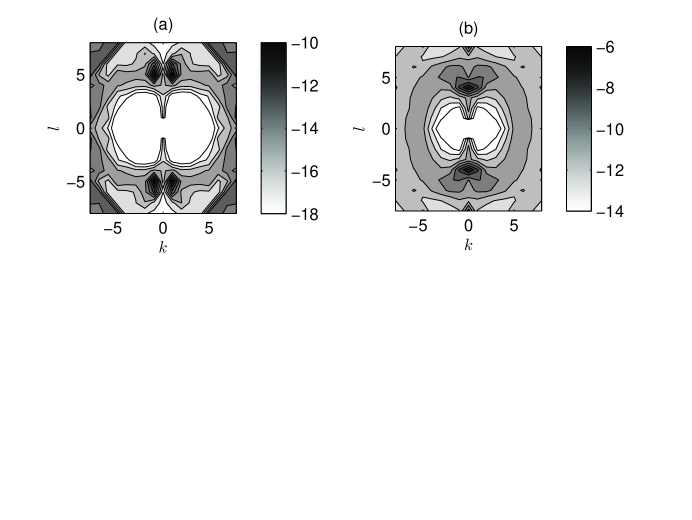
Figure 13: Time averaged energy power spectra, $\log(\hat{E}(k,l))$, obtained from the ensemble quasi-linear (EQL) simulations at (a) $\varepsilon/\varepsilon_{c}=4$ and (b) $\varepsilon/\varepsilon_{c}=50$ or $\varepsilon=3.3\varepsilon_{nl}$. There is a very good agreement with the corresponding spectra obtained from the non-linear (NL) simulations (cf. figures 2-3).

The second transition in which zonal jets emerge is more intriguing. The stability equation (20) predicts that the zonal structures become S3T unstable at $\varepsilon_{sz}=5.2\varepsilon_{c}$. As discussed in the previous section, the finite amplitude zonal jet equilibria are structurally unstable and the flow stays on the attractor of the non-zonal traveling wave equilibria (cf. figure 10). We determined that the jet equilibria are structurally unstable for $\varepsilon_{sz}<\varepsilon<\varepsilon_{nl}$. When $\varepsilon>\varepsilon_{nl}$, the non-zonal traveling wave equilibria become S3T unstable while at these parameter values the S3T system has mixed zonal jet-traveling wave equilibria which are stable (cf. figure 12). In both NL and EQL simulations, similar mixed zonal flow-traveling wave structures are evident (cf. figures 3, 13). However, there is a small discrepancy regarding the second transition between the EQL and NL simulations, as the energy input rate threshold for the emergence of jets is slightly larger in the NL simulations compared to the corresponding EQL threshold (cf. figure 1). This discrepancy possibly occurs due to the fact that the exchange of instabilities between the mixed jet-traveling wave equilibria and the pure traveling wave equilibria depends on the equilibrium structure $[Z^{E},C^{E}]$. Small changes for example in $C^{E}$ that might be caused by the eddy-eddy terms neglected in S3T can cause the exchange of instabilities to occur at slightly different energy input rates. It was shown in a recent study that when the effect of the eddy-eddy terms is taken into account by obtaining $C^{E}$ directly from the nonlinear simulations, the S3T stability analysis performed on this corrected equilibrium states accurately predicts the energy input rate for the emergence of jets in the nonlinear simulations (Constantinou et al., 2013). The power spectrum obtained from the EQL simulations for $\varepsilon=3.3\varepsilon_{nl}$ (cf. figure 13b) shows that both the scale and the amplitude of the zonal jets is captured by S3T. Such an agreement again holds for a wide range of energy input rates, as the zmf indices obtained from the EQL and the NL simulations indicate. In summary, S3T predicts the characteristics of both non-zonal propagating structures and of zonal jets in the non-linear simulations.

7 Discussion-conclusions

A theory for the emergence of zonal jets and non-zonal coherent structures in barotropic beta-plane turbulence is presented in this work. This is one of the simplest models that retains the relevant dynamics of self-organization of turbulence into large scale coherent structures and is a standard and extensively studied testbed for theories regarding the emergence and maintenance of zonal jets and coherent structures in planetary flows.

Non-linear simulations of a stochastically forced barotropic beta-plane channel show two major flow transitions as the energy input rate of the forcing increases. In the first, the translational symmetry in the flow is broken in both directions with the emergence of propagating coherent non-zonal waves that approximately follow the Rossby wave dispersion. The power in these non-zonal structures increases with the energy input rate until the second transition occurs with the emergence of robust zonal jets. Although after the second transition the zonal jets contain over half the energy in the flow, there is significant power in the non-zonal structures, which remain coherent and propagate in the retrograde direction with phase speeds that do not satisfy the Rossby wave dispersion.

The two flow transitions and the characteristics of both the non-zonal structures and the zonal jets are then investigated using a proper generalization of Stochastic Structural Stability Theory (S3T). In S3T, the turbulent flow dynamics and statistics are expressed as a systematic cumulant expansion which is truncated at second order. With the interpretation of the ensemble average as a Reynolds average over the fast turbulent eddies adopted in this work, the second order cumulant expansion results in a closed, non-linear dynamical system that governs the joint evolution of slowly varying, spatially localized coherent structures with the second order statistics of the rapidly evolving turbulent eddies. The fixed points of this autonomous, deterministic non-linear system define statistical equilibria, the stability of which are amenable to the usual treatment of linear and non-linear stability analysis.

The linear stability of the homogeneous S3T equilibrium with no mean velocity was examined analytically. Structural instability was found to occur for perturbations with smaller scale than the forcing, when the energy input rate $\tilde{\varepsilon}=\varepsilon K_{f}^{2}/r^{3}$ is larger than a certain threshold $\tilde{\varepsilon}_{c}$ that depends on $\tilde{\beta}=\beta/(rK_{f})$. It was found that when $\tilde{\beta}$ is small or order one, both zonal jets and non-zonal structures are unstable when the energy input rate is larger than $\tilde{\varepsilon}_{c}$, with the maximum growth rate occurring for stationary zonal structures. When $\tilde{\beta}$ is large, non-zonal structures first become unstable as the input rate increases past $\tilde{\varepsilon}_{c}$ with zonal jet structures becoming unstable at larger energy input rates. The maximum growth rate occurs in this case for non-zonal structures that propagate in the retrograde direction. These waves follow the Rossby wave dispersion for low supercritical values of the energy input rate, but propagate with different phase speeds at higher supercriticality. The equilibration of the unstable, exponentially growing coherent structures for large $\tilde{\beta}$ was then studied through numerical integrations of the S3T dynamical system. When the forcing amplitude is slightly supercritical, the finite amplitude traveling wave equilibrium has a structure close to the corresponding unstable non-zonal perturbation with the same scale. When the forcing amplitude is highly supercritical, the instabilities equilibrate to mixed states consisting of strong zonal jets with smaller amplitude traveling waves embedded in them.

The predictions of S3T were then compared to the results that obtain in the non-linear simulations. The critical threshold above which coherent non-zonal structures are unstable according to the stability analysis of the S3T system was found to be in excellent agreement with the critical value above which non-zonal structures acquire significant power in the non-linear simulations. The scale, phase speed and amplitude of the dominant structures in the non-linear simulations were also found to correspond to the structures predicted by S3T. In addition, the threshold for the emergence of jets, which is identified in S3T as the energy input rate at which an S3T stable, finite amplitude zonal jet equilibrium exists, was found to roughly match the corresponding threshold for jet formation in the non-linear simulations, with the emerging jet scale and amplitude being accurately obtained using S3T.

In summary, S3T predicts the two regime transitions in the turbulent flow as the energy input rate is increased: the emergence of coherent, propagating non-zonal structures and the emergence of zonal jets. It also predicts the characteristics of the emerging structures (their scales and their phase speed), as well as their amplitude. These results provide a concrete example that large scale structure in barotropic turbulence, whether it is zonal jets or non-zonal coherent structures, can arise from systematic self-organization of the turbulent Reynolds stresses by spectrally non-local interactions and in the absence of a turbulent cascade. The analysis reveals that the coherent structures emerge as unstable modes of the homogeneous statistical equilibrium. This instability shares the universal properties of pattern formation. In this work we have shown that the emergence of striped patterns (zonal jets) is preceded by the emergence of oscillating patterns (propagating waves). The analogy with pattern formation and the universality of the underlying dynamics may prove fruitful for understanding the domain of attraction of the non-zonal equilibria, as was previously done for the case of convection (Busse, 1978). This is part of ongoing research efforts by the authors and will be reported in the future.

Finally, we note that some of the characteristics of the coherent structures found in the barotropic beta-plane model may not accurately reproduce the characteristics of observed structures in the atmosphere or ocean. This should be no surprise, since the barotropic model lacks some of the important physics (baroclinicity, etc). For example, the oceanic vortex rings do not resemble the same plane wave or compact support structure of the coherent structures reported in this study. However, similarly with the structures that form under S3T dynamics, the vortex rings share the characteristic that they act as a long-lived repository of energy in the turbulent flow. Therefore their connection to the reported coherent structures needs to be further elucidated and is an attractive venue for future research.

This research was supported by the EU FP-7 under the PIRG03-GA-2008-230958 Marie Curie Grant. The authors acknowledge the hospitality of the Aspen Center for Physics supported by the NSF (under grant No. 1066293), where part of this work was done. The authors would also like to thank Navid Constantinou, Brian Farrell, James Cho, Freddy Bouchet and Brad Marston for fruitful discussions.

Appendix A Physical parameters for the Earth’s atmosphere and ocean and for the Jovian atmosphere

In this Appendix we discuss the relevant physical parameters (the forcing length scale, the dissipation time scale and the values of $\beta$) for the Earth’s atmosphere and ocean and for the Jovian atmosphere. For the Earth’s midlatitude atmosphere ($\beta=2\cdot 10^{-11}~{}\mbox{m}^{-1}\mbox{s}^{-1}$), we assume that the energy is injected at the cyclone scale of $1/K_{f}=1000~{}\mbox{km}$ and that the eddy dissipation time scale at midlatitudes is $1/r=10~{}\mbox{days}$. In addition, an energy transfer from the mean to the eddies of the order of $1.3~{}\mbox{Wm}^{-2}$ is typically found in studies of the Lorenz cycle in the atmosphere, while there is also another $20~{}\mbox{Wm}^{-2}$ available through diabatic heating (Peixoto & Oort, 1992). Assuming that a small fraction of the order of 5% is transferred into large scale eddies, we obtain a total amount of $2.3~{}\mbox{Wm}^{-2}$, which when injected over the troposphere with a scale height of 8 km, corresponds to an energy injection rate $\varepsilon=3\cdot~{}10^{-4}~{}\mbox{m}^{2}\mbox{s}^{-3}$. For the Earth’s ocean, we assume that the eddy energy is injected at the deformation scale $1/K_{f}=20~{}\mbox{km}$, while we consider that the eddy dissipation time scale is $1/r=1000~{}\mbox{days}$ (Berloff et al., 2009) and the energy injection rate is $\varepsilon=10^{-9}~{}\mbox{m}^{2}\mbox{s}^{-3}$ (Sukariansky et al., 2007). For the Jovian atmosphere at midlatitudes ($\beta=2.5\cdot 10^{-12}~{}\mbox{m}^{-1}\mbox{s}^{-1}$), we assume that energy is injected at the scale of convective storms $1/K_{f}=100~{}\mbox{km}$ with a rate $\varepsilon=0.5\cdot 10^{-5}~{}\mbox{m}^{2}\mbox{s}^{-3}$ (Galperin et al., 2013). Since the eddy dissipation rate is not known, we obtain an estimate by assuming that the observed root mean square velocity fluctuations $U_{rms}$ satisfy $U_{rms}^{2}=\varepsilon/r$. Taking $U_{rms}=50~{}\mbox{ms}^{-1}$ (Galperin et al., 2013), we obtain $1/r=5800~{}\mbox{days}$. It should be noted that these values are indicative order of magnitude estimates.

Appendix B Calculation of the dispersion relation and its properties

In this Appendix we derive the dispersion relation (20), which determines the stability of zonal as well as non-zonal perturbations in homogeneous turbulence. We follow closely the treatment of Srinivasan & Young (2012). We first rewrite (14), (18) in terms of the variables $\tilde{x}=x_{1}-x_{2}$, $\overline{x}=(1/2)(x_{1}+x_{2})$, $\tilde{y}=y_{1}-y_{2}$ and $\overline{y}=(1/2)(y_{1}+y_{2})$. The derivatives transform into this new system of coordinates to $\partial_{x_{i}}=(1/2)\partial_{\overline{x}}+(-1)^{i+1}\partial_{\tilde{x}}$, $\partial_{y_{i}}=(1/2)\partial_{\overline{y}}+(-1)^{i+1}\partial_{\tilde{y}}$, $\Delta_{i}=\tilde{\Delta}+(1/4)\overline{\Delta}+(-1)^{i+1}\partial_{\tilde{y}\overline{y}}^{2}+(-1)^{i+1}\partial_{\tilde{x}\overline{x}}^{2}$, with $\tilde{\Delta}=\partial_{\tilde{x}\tilde{x}}^{2}+\partial_{\tilde{y}\tilde{y}}^{2}$ and $\overline{\Delta}=\partial_{\overline{x}\overline{x}}^{2}+\partial_{\overline{y}\overline{y}}^{2}$. It is also convenient to introduce the streamfunction covariance $S(\tilde{x},\overline{x},\tilde{y},\overline{y})\equiv\left<\psi_{1}^{\prime}\psi_{2}^{\prime}\right>$, which is related to $C(\tilde{x},\overline{x},\tilde{y},\overline{y})$ via:

$$C=\left<\zeta_{1}^{\prime}\zeta_{2}^{\prime}\right>=\left<\Delta_{1}\psi_{1}^{\prime}\Delta_{2}\psi_{2}^{\prime}\right>=\Delta_{1}\Delta_{2}S=\left[\left({\tilde{\Delta}}+{1\over 4}\overline{\Delta}\right)^{2}-\left(\partial_{\tilde{x}\overline{x}}^{2}+\partial_{\tilde{y}\overline{y}}^{2}\right)^{2}\right]S.$$ (26)

Equations (14), (18) then become in the absence of hyper-viscosity ($\nu=0$):

$$\left[\partial_{t}+\overline{U}\partial_{\overline{x}}+\tilde{U}\partial_{\tilde{x}}+\overline{V}\partial_{\overline{y}}+\tilde{V}\partial_{\tilde{y}}\right]C+\left[(\beta+\overline{Z}_{y})\partial_{\overline{x}}+\tilde{Z}_{y}\partial_{\tilde{x}}-\overline{Z}_{x}\partial_{\overline{y}}-\tilde{Z}_{x}\partial_{\tilde{y}}\right]\left(\tilde{\Delta}+\frac{1}{4}\overline{\Delta}\right)S$$ (27)

$$- \left[2(\beta+\overline{Z}_{y})\partial_{\tilde{x}}+\frac{1}{2}\tilde{Z}_{y}\partial_{\overline{x}}-2\overline{Z}_{x}\partial_{\tilde{y}}-\frac{1}{2}\tilde{Z}_{x}\partial_{\overline{y}}\right]\left(\partial_{\tilde{x}\overline{x}}^{2}+\partial_{\tilde{y}\overline{y}}^{2}\right)S=-2rC+\Xi,$$

$$\partial_{t}Z+U\partial_{x}Z+V(\beta+\partial_{y}Z)=(\partial_{\tilde{x}\overline{y}}^{2}-\partial_{\tilde{y}\overline{x}}^{2})(\partial_{\tilde{x}\overline{x}}^{2}+\partial_{\tilde{y}\overline{y}}^{2})S|_{\tilde{x}=\tilde{y}=0}-rZ,$$ (28)

where $(\overline{U},\overline{V})=(1/2)(U_{1}+U_{2},V_{1}+V_{2})$, $(\tilde{U},\tilde{V})=(U_{1}-U_{2},V_{1}-V_{2})$, $(\overline{Z}_{x},\overline{Z}_{y})=(1/2)(\partial_{x_{1}}+\partial_{x_{2}},\partial_{y_{1}}+\partial_{y_{2}})Z$ and $(\tilde{Z}_{x},\tilde{Z}_{y})=(\partial_{x_{1}}-\partial_{x_{2}},\partial_{y_{1}}-\partial_{y_{2}})Z$.

The forcing covariance $\Xi$ is homogeneous and as a result it depends only on the difference coordinates, $\tilde{x}$ and $\tilde{y}$. It can then be readily shown from (27)-(28), that the state with no coherent flow ($U^{E}=V^{E}=Z^{E}=0$) and with the homogeneous vorticity covariance $C^{E}(\tilde{x},\tilde{y})=\Xi/(2r)$ (implying also that the streamfunction covariance $S^{E}$ is homogenous) is a fixed point of the S3T system. The stability of this homogeneous equilibrium, can be addressed by first linearizing the S3T system about it:

$$\partial_{t}\delta C = -\left(\delta\tilde{U}\partial_{\tilde{x}}+\delta\tilde{V}\partial_{\tilde{y}}\right)C^{E}-\left(\delta\tilde{Z}_{y}\partial_{\tilde{x}}-\delta\tilde{Z}_{x}\partial_{\tilde{y}}\right)\tilde{\Delta}S^{E}$$ (29)

$$- \beta\left\{\left[\tilde{\Delta}+\frac{1}{4}\overline{\Delta}\right]\partial_{\overline{x}}-2(\partial_{\tilde{x}\overline{x}}^{2}+\partial_{\tilde{y}\overline{y}}^{2})\partial_{\tilde{x}}\right\}\delta S-2r\delta C,$$

$$\partial_{t}\delta Z=-\beta\delta V+(\partial_{\tilde{x}\overline{y}}^{2}-\partial_{\tilde{y}\overline{x}}^{2})(\partial_{\tilde{x}\overline{x}}^{2}+\partial_{\tilde{y}\overline{y}}^{2})\delta S|_{\tilde{x}=\tilde{y}=0}-r\delta Z,$$ (30)

where $\delta Z$, $\delta\tilde{U}$, $\delta\tilde{V}$, $\delta\tilde{Z}_{x}$, $\delta\tilde{Z}_{y}$, $\delta C$ and $\delta S$ are small perturbations in the ensemble mean vorticity, velocities and vorticity gradients and in the eddy vorticity and streamfunction covariances respectively, and then performing an eigenanalysis of the linearized equations (29)-(30).

We consider a harmonic vorticity perturbation of the form $\delta Z=\mathrm{e}^{\mathrm{i}nx+\mathrm{i}my}\mathrm{e}^{\sigma t}$, for which:

$$[\delta\tilde{U},\delta\tilde{V},\delta\tilde{Z}_{x},\delta\tilde{Z}_{y}]=-2\left[\frac{m}{n^{2}+m^{2}},-\frac{n}{n^{2}+m^{2}},n,m\right]\sin\left(\frac{n\tilde{x}}{2}+\frac{m\tilde{y}}{2}\right)\mathrm{e}^{\mathrm{i}n\overline{x}+\mathrm{i}m\overline{y}}\mathrm{e}^{\sigma t}.$$ (31)

Taking the same form for the streamfunction covariance perturbation $\delta S=S_{nm}(\tilde{x},\tilde{y})\mathrm{e}^{\mathrm{i}n\overline{x}+\mathrm{i}m\overline{y}}\mathrm{e}^{\sigma t}$ and inserting it in (29)-(30) along with (31) yields:

$$\left\{(\sigma+2r)\left[\left(\tilde{\Delta}-\frac{N^{2}}{4}\right)^{2}+\Delta_{+}^{2}\right]-2\mathrm{i}\beta\Delta_{+}\partial_{\tilde{x}}+\mathrm{i}n\beta\left(\tilde{\Delta}-\frac{N^{2}}{4}\right)\right\}S_{nm}$$ (32)

$$= \frac{2}{N^{2}}\sin\left(\frac{n\tilde{x}}{2}+\frac{m\tilde{y}}{2}\right)\left(m\partial_{\tilde{x}}-n\partial_{\tilde{y}}\right)\left[\tilde{\Delta}^{2}+N^{2}\tilde{\Delta}\right]S^{E},$$

$$-(\sigma+r)N^{2}+\mathrm{i}n\beta=N^{2}\left(m\partial_{\tilde{x}}-n\partial_{\tilde{y}}\right)\Delta_{+}S_{nm}|_{\tilde{x}=\tilde{y}=0},$$ (33)

where $N^{2}=n^{2}+m^{2}$, $\Delta_{+}=n\partial_{\tilde{x}}+m\partial_{\tilde{y}}$ and $C^{E}=\Xi/2r=\tilde{\Delta}^{2}S^{E}$ is the equilibrium vorticity covariance with zero mean flow.

Defining the Fourier transform of ${S}_{nm}(\tilde{x},\tilde{y})$ by

$$\hat{S}_{nm}(k,l)={1\over 2\pi}\int_{-\infty}^{\infty}\int_{-\infty}^{\infty}{S}_{nm}(\tilde{x},\tilde{y})\mathrm{e}^{-\mathrm{i}k\tilde{x}-\mathrm{i}l\tilde{y}}\mathrm{d}\tilde{x}\mathrm{d}\tilde{y}~{},$$ (34)

we obtain from (32) that the Fourier component $\hat{S}_{nm}$ satisfies:

$$\hat{S}_{nm} = \frac{(mk_{-}-nl_{-})K_{-}^{2}(K_{-}^{2}/N^{2}-1)\hat{S}^{E}(k_{-},l_{-})}{2\mathrm{i}\beta k(kn+ml)-\mathrm{i}n\beta(K_{+}^{2}+K_{-}^{2})/2+(\sigma+2r)K_{+}^{2}K_{-}^{2}}$$ (35)

$$- \frac{(mk_{+}-nl_{+})K_{+}^{2}(K_{+}^{2}/N^{2}-1)\hat{S}^{E}(k_{+},l_{+})}{2\mathrm{i}\beta k(kn+ml)-\mathrm{i}n\beta(K_{+}^{2}+K_{-}^{2})/2+(\sigma+2r)K_{+}^{2}K_{-}^{2}},$$

with $k_{\pm}=k\pm n/2$, $l_{\pm}=l\pm m/2$, $K_{\pm}^{2}=k_{\pm}^{2}+l_{\pm}^{2}$ and $K^{2}=k^{2}+l^{2}$. $\hat{S}^{E}=\hat{\Xi}/(2rK^{4})$ is the Fourier transform of $S^{E}$, and $\hat{\Xi}$ is the Fourier transform of $\Xi$. In addition, (33) becomes:

$$\mathrm{i}n\beta-(\sigma+r)N^{2}=-{N^{2}\over 2\pi}\int_{-\infty}^{\infty}\int_{-\infty}^{\infty}\left[nm(k^{2}-l^{2})+(m^{2}-n^{2})kl\right]\hat{S}_{nm}\mathrm{d}k\mathrm{d}l=\Lambda_{+}-\Lambda_{-},$$ (36)

where

$$\Lambda_{\pm}={1\over 2\pi}\int_{-\infty}^{\infty}\int_{-\infty}^{\infty}\frac{\left[nm(k^{2}-l^{2})+(m^{2}-n^{2})kl\right](mk_{\pm}-nl_{\pm})K_{\pm}^{2}(K_{\pm}^{2}-N^{2})\hat{S}^{E}(k_{\pm},l_{\pm})}{2\mathrm{i}\beta k(kn+ml)-\mathrm{i}n\beta(K_{+}^{2}+K_{-}^{2})/2+(\sigma+2r)K_{+}^{2}K_{-}^{2}}\mathrm{d}k\mathrm{d}l.$$ (37)

Equation (36) can be further simplified by noting that because the choice of $\mathbf{x}_{1}$ and $\mathbf{x}_{2}$ is arbitrary, the forcing covariance satisfies the exchange symmetry $\Xi(x_{1},x_{2},y_{1},y_{2})=\Xi(x_{2},x_{1},y_{2},y_{1})$. In terms of the new variables, the exchange symmetry is written as $\Xi(\tilde{x},\overline{x},\tilde{y},\overline{y})=\Xi(-\tilde{x},\overline{x},-\tilde{y},\overline{y})$, and consequently $\hat{\Xi}$ satisfies $\hat{\Xi}(-k,-l)=\hat{\Xi}(k,l)$. As a result:

$$\Lambda_{+}=-\Lambda_{-}.$$ (38)

Using (38) and shifting the axes in the resulting integrals ($k\rightarrow k+n/2$ and $l\rightarrow l+m/2$), reduces (36) to the following dispersion relation:

$$\int_{-\infty}^{\infty}\int_{-\infty}^{\infty}\frac{(mk-nl)\left[nm(k_{+}^{2}-l_{+}^{2})+(m^{2}-n^{2})k_{+}l_{+}\right]K^{2}(K^{2}-N^{2})\hat{S}^{E}(k,l)}{2\mathrm{i}\beta k_{+}(k_{+}n+l_{+}m)-\mathrm{i}n\beta\left(K^{2}+K_{s}^{2}\right)/2+(\sigma+2r)K^{2}K_{s}^{2}}\mathrm{d}k\mathrm{d}l$$ (39)

$$= \pi(\sigma+r)N^{2}-\mathrm{i}\pi n\beta,$$

where $K_{s}^{2}=(k+n)^{2}+(l+m)^{2}$. The corresponding dispersion relation on a periodic box, can be readily calculated by simply substituting the integrals in (39) by finite sums of integer wavenumbers. For a mirror symmetric forcing obeying:

$$\hat{\Xi}(-k,l)=\hat{\Xi}(k,l),$$ (40)

the eigenvalues $\sigma$ satisfy the symmetries (24). In order to show this, we consider (39) for $\sigma_{(-n,m)}$ and change the sign of $k$ in the integral to obtain:

$$\int_{-\infty}^{\infty}\int_{-\infty}^{\infty}\frac{(mk-nl)\left[nm(k_{+}^{2}-l_{+}^{2})+(m^{2}-n^{2})k_{+}l_{+}\right]K^{2}(K^{2}-N^{2})\hat{S}^{E}(-k,l)}{-2\mathrm{i}\beta k_{+}(k_{+}n+l_{+}m)+\mathrm{i}n\beta\left(K^{2}+K_{s}^{2}\right)/2+(\sigma_{(-n,m)}+2r)K^{2}K_{s}^{2}}\mathrm{d}k\mathrm{d}l$$ (41)

$$= \pi(\sigma_{(-n,m)}+r)N^{2}+\mathrm{i}\pi n\beta.$$

Taking the conjugate of (41) and using the mirror symmetry (40) yields (39) and therefore $\sigma_{(-n,m)}=\sigma_{(n,m)}^{*}$. Similarly, it can be readily shown by considering (39) for $\sigma_{(n,-m)}$ and changing the sign of $l$ in the integral, that $\sigma_{(n,-m)}=\sigma_{(n,m)}$.

References

- Bakas & Ioannou (2011) Bakas, N. A. & Ioannou, P. J. 2011 Structural stability theory of two-dimensional fluid flow under stochastic forcing. J. Fluid Mech. 682, 332–361.
- Bakas & Ioannou (2013a) Bakas, N. A. & Ioannou, P. J. 2013a Emergence of large scale structure in barotropic beta-plane turbulence. Phys. Rev. Lett. 110, 224501.
- Bakas & Ioannou (2013b) Bakas, N. A. & Ioannou, P. J. 2013b On the mechanism underlying the spontaneous emergence of barotropic zonal jets. J. Atmos. Sci. 70, 2251–2271.
- Berloff et al. (2009) Berloff, P., Kamenkovich, I. & Pedlosky, J. 2009 A mechanism of formation of multiple zonal jets in the oceans. J. Fluid Mech. 628, 395–425.
- Bernstein (2009) Bernstein, J. 2009 Dynamics of turbulent jets in the atmosphere and ocean. PhD thesis, Harvard University.
- Bernstein & Farrell (2010) Bernstein, J. & Farrell, B. F. 2010 Low-frequency variability in a turbulent baroclinic jet: Eddy-mean flow interactions in a two-level model. J. Atmos. Sci. 67, 452–467.
- Bouchet et al. (2013) Bouchet, F., Nardini, C. & Tangarife, T. 2013 Kinetic theory of jet dynamics in the stochastic barotropic and 2d navier-stokes equations. arXiv preprint arXiv:1305.0877 .
- Bouchet & Sommeria (2002) Bouchet, F. & Sommeria, J. 2002 Emergence of intense jets and Jupiter’s Great Red Spot as maximum-entropy structures. J. Fluid Mech. 464, 165–207.
- Bouchet & Venaille (2012) Bouchet, F. & Venaille, A. 2012 Statistical mechanics of two-dimensional and geophysical flows. Phys. Rep. 515 (5), 227–295.
- Busse (1978) Busse, F. H. 1978 Nonlinear properties of convection. Rep. Prog. Phys. 41, 1929–1967.
- Chavanis & Sommeria (1998) Chavanis, P. H. & Sommeria, J. 1998 Classification of robust isolated vortices in two-dimensional hydrodynamics. J. Fluid Mech. 356, 259–296.
- Chelton et al. (2007) Chelton, D. B., Schlax, M. G., Samelson, R. M. & de Szoeke, R. A. 2007 Global observations of large oceanic eddies. Geophys. Res. Lett. 34, L12607.
- Cho & Polvani (1996) Cho, J. Y. K & Polvani, L. M. 1996 The morphogenesis of bands and zonal winds in the atmospheres on the giant outer planets. Science 273, 335–337.
- Constantinou et al. (2013) Constantinou, N. C., Farrell, B. F. & Ioannou, P. J. 2013 Emergence and equilibration of jets in beta-plane turbulence: applications to Stochastic Structural Stability Theory. J. Atmos. Sci. (sub judice, arXiv:1208.5665 [physics.flu-dyn]).
- Cross & Greenside (2009) Cross, M. & Greenside, H. 2009 Pattern Formation and Dynamics in Nonequilibrium Systems. Cambridge University Press.
- Danilov & Gurarie (2004) Danilov, S. & Gurarie, D. 2004 Scaling, spectra and zonal jets in beta plane turbulence. Phys. of Fluids 16, 2592–2603.
- DelSole (2004) DelSole, T. 2004 Stochastic models of quasigeostrophic turbulence. Surv. Geophys. 25, 107–194.
- DelSole & Farrell (1996) DelSole, T. & Farrell, B. F. 1996 The quasi-linear equilibration of a thermally maintained, stochastically excited jet in a quasigeostrophic model. J. Atmos. Sci. 53, 1781–1797.
- Di Nitto et al. (2013) Di Nitto, G, Espa, S & Cenedese, A 2013 Simulating zonation in geophysical flows by laboratory experiments. Physics of Fluids 25, 086602.
- Dubrulle & Nazarenko (1997) Dubrulle, B. & Nazarenko, S. 1997 Interaction of turbulence and large-scale vortices in incompressible 2D fluids. Physica D 110, 123–138.
- Espa et al. (2010) Espa, S., Di Nitto, G. & Cenedese, A. 2010 The emergence of zonal jets in forced rotating shallow water turbulence: A laboratory study. EPL 92, 10.1209/0295–5075/92/34006.
- Farrell & Ioannou (1993a) Farrell, B. F. & Ioannou, P. J. 1993a Stochastic dynamics of baroclinic waves. J. Atmos. Sci. 50, 4044–4057.
- Farrell & Ioannou (1993b) Farrell, B. F. & Ioannou, P. J. 1993b Stochastic forcing of perturbation variance in unbounded shear and deformation flows. J. Atmos. Sci. 50, 200–211.
- Farrell & Ioannou (1993c) Farrell, B. F. & Ioannou, P. J. 1993c Stochastic forcing of the linearized Navier- Stokes equations. Phys. Fluids 5, 2600–2609.
- Farrell & Ioannou (2003) Farrell, B. F. & Ioannou, P. J. 2003 Structural stability of turbulent jets. J. Atmos. Sci. 60, 2101–2118.
- Farrell & Ioannou (2007) Farrell, B. F. & Ioannou, P. J. 2007 Structure and spacing of jets in barotropic turbulence. J. Atmos. Sci. 64, 3652–3655.
- Farrell & Ioannou (2008) Farrell, B. F. & Ioannou, P. J. 2008 Formation of jets in baroclinic turbulence. J. Atmos. Sci. 65, 3352–3355.
- Farrell & Ioannou (2009a) Farrell, B. F. & Ioannou, P. J. 2009a Emergence of jets from turbulence in the shallow-water equations on an equatorial beta-plane. J. Atmos. Sci. 66, 3197–3207.
- Farrell & Ioannou (2009b) Farrell, B. F. & Ioannou, P. J. 2009b A stochastic structural stability theory model of the drift wave-zonal flow system. Physics of Plasmas 16, 112903.
- Farrell & Ioannou (2009c) Farrell, B. F. & Ioannou, P. J. 2009c A theory of baroclinic turbulence. J. Atmos. Sci. 66, 2444–2454.
- Farrell & Ioannou (2012) Farrell, B. F. & Ioannou, P. J. 2012 Dynamics of streamwise rolls and streaks in turbulent wall–bounded shear flow. J. Fluid Mech. 708, 149–196.
- Fjörtöft (1953) Fjörtöft, R. 1953 On the changes in the spectral distribution of kinetic evergy for two-dimensional, non-divergent flow. Tellus 5, 120–140.
- Galperin et al. (2010) Galperin, B. H., Sukoriansky, S. & Dikovskaya, N. 2010 Geophysical flows with anisotropic turbulence and dispersive waves: flows with a -effect. Ocean Dyn. 60, 427–441.
- Galperin et al. (2006) Galperin, B. H., Sukoriansky, S., Dikovskaya, N., Read, P., Yamazaki, Y. & Wordsworth, R. 2006 Anisotropic turbulence and zonal jets in rotating flows with a -effect. Nonlinear Proc. Geoph. 13, 83–98.
- Galperin et al. (2013) Galperin, B. H., Young, R. M., S., Sukoriansky, Dikovskaya, N., L., Read P., J., Lancaster A. & D., Armstrong 2013 Cassini observations reveal a regime of zonostrophic macroturbulence on Jupiter. Icarus in press.
- Huang et al. (2001) Huang, H. P., Galperin, B. H. & Sukoriansky, S. 2001 Anisotropic spectra in two-dimensional turbulence on the surface of a rotating sphere. Phys. Fluids 13, 225–240.
- Huang & Robinson (1998) Huang, H. P. & Robinson, W. A. 1998 Two-dimensional turbulence and persistent zonal jets in a global barotropic model. J. Atmos. Sci. 55, 611–632.
- Ingersoll (1990) Ingersoll, A. P. 1990 Atmospheric dynamics of the outer planets. Science 248, 308–315.
- Laval et al. (2003) Laval, J.-P., Dubrulle, B. & McWilliams, J. C. 2003 Langevin models of turbulence: Renormalization group, distant interaction algorithms or rapid distortion theory? Phys. Fluids 15, 1327–1339.
- Laval et al. (2000) Laval, J. P., Dubrulle, B. & Nazarenko, S. 2000 Dynamical modeling of sub-grid scales in 2D turbulence. Physica D 142, 231–235.
- Marston (2010) Marston, J. B. 2010 Statistics of the general circulation from cumulant expansions. Chaos 20, 041107.
- Marston (2012) Marston, J. B. 2012 Planetary atmospheres as nonequilibrium condensed matter. Annu. Rev. Condens. Matter Phys. 3, 285–310.
- Marston et al. (2008) Marston, J. B., Conover, E. & Schneider, T. 2008 Statistics of an unstable barotropic jet from a cumulant expansion. J. Atmos. Sci. 65, 1955–1966.
- Maximenko et al. (2005) Maximenko, N., Bang, B. & Sasaki, H. 2005 Observational evidence of alternating zonal jets in the world ocean. Geophys. Res. Lett. 32, L12607.
- Miller (1990) Miller, J. 1990 Statistical mechanics of Euler equation in two-dimensions. Phys. Rev. Lett. 65, 2137–2140.
- Nadiga (2006) Nadiga, B. 2006 On zonal jets in oceans. Geophys. Res. Lett. 33, L10601.
- Nazarenko & Quinn (2009) Nazarenko, S. & Quinn, B. 2009 Triple cascade behavior in quasigeostrophic and drift turbulence and generation of zonal jets. Phys. Rev. Letters 103, 118501.
- Nozawa & Yoden (1997) Nozawa, T. & Yoden, Y. 1997 Formation of zonal band structure in forced two-dimensional turbulence on a rotating sphere. Phys. Fluids 9, 2081–2093.
- O’Gorman & Schneider (2007) O’Gorman, P. A. & Schneider, T. 2007 Recovery of atmospheric flow statistics in a general circulation model without nonlinear eddy-eddy interactions. Geophys. Res. Lett. 34, L22801.
- Onsager (1949) Onsager, L. 1949 Statistical hydrodynamics. Nuovo Cimento 6, 249–286.
- Parker & Krommes (2013) Parker, J. B. & Krommes, J. A. 2013 Zonal flow as pattern formation: Merging jets and the ultimate jet length scale arXiv: 1301.5059 [physics.ao-ph].
- Peixoto & Oort (1992) Peixoto, J. P. & Oort, A. H. 1992 Physics of Climate. American Institute of Physics.
- Rayleigh (1916) Rayleigh, Lord 1916 On the convective currents in a horizontal layer of fluid when the higher temperature is on the under side. Phil. Mag. 32, 529–546.
- Read et al. (2004) Read, P. L., Yamazaki, Y. H., Lewis, S. R., Williams, P. D., Miki-Yamazaki, K., Sommeria, J., Didelle, H. & Fincham, A. 2004 Jupiter’s and Saturn’s convectively driven banded jets in the laboratory. Geophys. Res. Lett. 87, 1961–1967.
- Rhines (1975) Rhines, P. B. 1975 Waves and turbulence on a beta plane. J. Fluid Mech. 69, 417–433.
- Robert & Sommeria (1991) Robert, R. & Sommeria, J. 1991 Statistical equilibrium states for two-dimensional flows. J. Fluid Mech. 229, 291–310.
- Shepherd (1987) Shepherd, T. G. 1987 A spectral view of nonlinear fluxes and stationary-transient interaction in the atmosphere. J. Atmos. Sci. 44, 1166–1178.
- Smith et al. (2002) Smith, K. S., Boccaletti, G., Henning, C. C., Marinov, L., Tam, C. Y., Held, I. M. & Vallis, G. K. 2002 Turbulent diffusion in the geostrophic inverse cascade. J. Fluid Mech. 469, 13–48.
- Srinivasan & Young (2012) Srinivasan, K. & Young, W. R. 2012 Zonostrophic instability. J. Atmos. Sci. 69, 1633–1656.
- Sukariansky et al. (2007) Sukariansky, S., Dikovskaya, N. & Galperin, B. 2007 On the arrest of inverse energy cascade and the Rhines scale. J. Atmos. Sci. 64, 3312–3327.
- Sukariansky et al. (2008) Sukariansky, S., Dikovskaya, N. & Galperin, B. 2008 Nonlinear waves in zonostrophic turbulence. Phys. Rev. Lett. 101, 178501.
- Tobias et al. (2011) Tobias, S. M., Dagon, K. & Marston, J. B. 2011 Astrophysical fluid dynamics via direct numerical simulation. Astrophys. J. 727, 127 doi: 10.1088/0004–637X/727/2/127.
- Vallis & Maltrud (1993) Vallis, G. K. & Maltrud, M. E. 1993 Generation of mean flows and jets on a beta plane and over topography. J. Phys. Oceanogr. 23, 1346–1362.
- Vasavada & Showman (2005) Vasavada, A. R. & Showman, A. P. 2005 Jovian atmospheric dynamics. An update after Galileo and Cassini. Rep. Prog. Phys. 68, 1935–1996.
- Venaille & Bouchet (2011) Venaille, A. & Bouchet, F. 2011 Oceanic rings and jets as statistical equilibrium states. J. Phys. Oceanogr. 41, 1860–1873.
- Weeks et al. (1997) Weeks, W. R., Trian, Y., Urbach, J. S., Ide, K., Swinney, H. L. & Ghil, M. 1997 Transitions between blocked and zonal flows in a rotating annulus. Science 278, 1598–1601.
- Williams (1978) Williams, G. P. 1978 Planetary circulations: 1. Barotropic representation of Jovian and terrestrial turbulence. J. Atmos. Sci. 35, 1399–1426.