A new observable to measure the top-quark mass at hadron colliders

Abstract

A new method to measure the top-quark mass in high energetic hadron collisions is presented. We use theoretical predictions calculated at next-to-leading order accuracy in quantum chromodynamics to study the (normalized) differential distribution of the $t\bar{t}+1\textnormal{\normalsize-jet}$ cross section with respect to its invariant mass $\sqrt{s_{t\bar{t}j}}$. The sensitivity of the method to the top-quark mass together with the impact of various theoretical and experimental uncertainties has been investigated and quantified. The new method allows for a complementary measurement of the top-quark mass parameter and has a high potential to become competitive in precision with respect to established approaches. Furthermore we emphasize that in the proposed method the mass parameter is uniquely defined through one-loop renormalization.

1 Introduction

With a mass of $173.2\pm 0.9$ GeV the top quark is the heaviest elementary fermion discovered so far Aaltonen:2012ra ; Abazov:2011pta ; Beringer:1900zz . In the Standard Model (SM) the large mass constrains the top-quark lifetime to become extremely short, inhibiting top-quark bound states to be formed. As an important consequence top quarks offer the unique possibility to study the properties of a quasi-free quark. Owing to its parity violating decay it is, for example, possible to analyze the top-quark polarization in difference to the lighter quarks where the spin information is typically diluted through the hadronization. In the SM the top-quark Yukawa coupling is very close to one. With the strongest coupling to the Higgs boson the top quark represents an ideal laboratory for detailed tests of the Higgs mechanism. Beyond the SM the top quark plays an important role in scenarios aiming to give an alternative explanation of spontaneous electroweak symmetry breaking (EWSB). Top-quark physics is thus a sensitive probe for precision tests of the SM but also for new physics searches. The Large Hadron Collider (LHC) will allow measurements of the top-quark properties with unmatched accuracy. In the SM the top-quark couplings are completely predicted through the gauge structure. The only free parameters in the top-quark sector are the matrix elements of the Cabbibo-Kobayashi-Maskawa (CKM) mixing matrix and the top-quark mass. The CKM matrix elements are highly constrained through indirect measurements. The LHC experiments will complement this picture through direct measurements of the CKM matrix elements in single top-quark production. Precise top-quark mass measurements are of high physics relevance. First, on its own right as the top-quark mass represents a fundamental parameter of the SM. Second, because its comparison with the mass of the recently observed resonance atlashiggs:2012gk ; cmshiggs:2012gu —assuming that the resonance is the long-sought Higgs boson—can be used to test the validity of the SM Heinemeyer:2006px since the $W$ boson mass, the top-quark mass and the Higgs boson mass are related in the SM. Very recently also the impact of the top-quark mass on the stability of the electroweak vacuum has been revisited Degrassi:2012ry ; Alekhin:2012py .

Quarks, in contrast to leptons, are colored objects which interact strongly in addition to the usual electroweak interactions. As a consequence quarks are not observed as free particles. They are confined into colorless hadrons. The natural way to measure quark masses is thus to treat them similarly to other couplings of the underlying theory: the couplings are measured through their influence on hadronic observables. More precisely, theoretical predictions are compared with measurements and the couplings are then obtained through a fit. For two examples where this idea has been applied in practice we refer to Refs. Bilenky:1998nk ; Langenfeld:2009wd . Since the parameters of a model are in general not observables by themselves their precise values depend on the renormalization scheme used to define them. Qualitatively renormalization controls which part of quantum corrections are already accounted for through the renormalized couplings measured in the experiments. As a consequence one needs at least a next-to-leading order (NLO) calculation—where quantum corrections appear for the first time in the theoretical predictions—to define unambiguously the renormalization scheme. In leading order (LO) different schemes cannot be distinguished and are formally equivalent in perturbation theory. In the case of heavy quark masses the most commonly used definitions are the pole mass $m_{q}^{\mbox{\scriptsize pole}}$ and the running mass $\overline{m}_{q}(\mu_{r})$. The former is defined as the pole of the renormalized quark propagator while the latter is defined through modified minimal subtraction ($\overline{\mbox{MS}}$). In the $\overline{\mbox{MS}}$ scheme the renormalization constants are chosen such that only the ultraviolet divergences together with the constant $-\gamma_{E}+\ln(4\pi)$ are removed through the renormalization program. (The constant $\gamma_{E}=0.577215\ldots$ denotes the Euler-Mascheroni constant.) Similar to the coupling constant of the strong interaction, the running mass $\overline{m}_{q}(\mu_{r})$ depends on the renormalization scale $\mu_{r}$. Physics should be independent of the mass definition used. However at any fixed order in perturbation theory a residual dependence on the mass definition as well as on the arbitrary renormalization scale $\mu_{r}$ remains. In specific cases, the $\mu_{r}$ dependence of the $\overline{\mbox{MS}}$ mass can be used to absorb certain logarithmically enhanced corrections and resum them to all orders within perturbation theory. This may lead to an improved behavior of the perturbative predictions (see for example Ref. Langenfeld:2009wd ). In top-quark physics the large top-quark mass naturally sets a large scale resulting in a small value of the QCD coupling $\alpha_{s}$ evaluated at $\mu_{r}=m_{t}^{\mbox{\scriptsize pole}}$ and we believe that the aforementioned scheme dependence is in general less important than for the lighter quarks. Nevertheless, if precise determinations of the top-quark mass are pursued, it is of major relevance to understand the quantitative extent of this qualitative argument. A discussion of different methods and approaches used to measure the top-quark mass will contribute in clarifying this statement.

Direct determinations of the top-quark mass have been performed at the Tevatron and LHC colliders. The top-quark mass is presently inferred by the kinematical reconstruction of the invariant mass of its decay products with techniques such as the matrix element or the template method (see e.g., Ref. Aaltonen:2012ra and references therein) or by its relation to the top-quark pair production cross section Langenfeld:2009wd . The top-quark mass derived from the kinematical reconstruction does not correspond to a well-defined renormalization scheme leading to a theoretical uncertainty in its interpretation. Nevertheless it is usually interpreted as the top-quark pole mass $m_{t}^{\mbox{\scriptsize pole}}$. The present results achieved using the kinematical reconstruction reach a higher precision ($m_{t}=173.2\pm 0.9$ GeV Aaltonen:2012ra ) than those which are extracted from the cross section measurements (e.g. $m_{t}^{\mbox{\scriptsize pole}}=173.3\pm 2.8$ GeV Alekhin:2012py using Ref. Aliev:2010zk ). The large experimental uncertainty of the mass determinations based on cross section measurements is a consequence of the sensitivity of the cross section on the top-quark mass. However we emphasize that in this measurement the renormalization scheme is unambiguously defined in difference to the determination based on the kinematical reconstruction. In particular using the cross section measurements a direct extraction of the running mass is possible. This was for the first time done in Ref. Langenfeld:2009wd and is currently repeated by the CMS and ATLAS collaborations. The experimental accuracy of the method is limited by the weak sensitivity of the cross section on the top-quark mass. Assuming an experimental accuracy of 5% on the cross section measurements a determination of the mass accurate to 1% could be envisaged.

Given the physical relevance of top-quark mass measurements it is important to employ alternative methods with similar or even better accuracy than the methods mentioned above. With the current accuracy of the mass measurements being better than one per cent this is a highly non-trivial task. In this work we advocate a new method to measure the top-quark mass in high energetic hadron collisions at the LHC. The mass dependence of the production of top-quark pairs in association with an additional jet is exploited. This process is sensitive to the top-quark mass since gluon radiation depends on the top-quark mass through threshold and cone effects. More precisely, we study the normalized $t\bar{t}+1\textnormal{\normalsize-jet}$ cross section differential in the invariant mass of the final state jets. In section 2 a detailed description of the observable is given together with a short discussion of the available theoretical predictions including an analysis of the theoretical uncertainties. Section 3 reports on a generic study of the observable at the particle level. In particular the major uncertainties of the method are investigated. We finally present our conclusions in section 4.

2 Top-quark pair production in association with a hard jet at NLO accuracy in QCD

The production process for top-quark pairs in association with a hard jet occurs with a large rate at the LHC. Together with the high statistics data samples based on the integrated luminosity of the runs at 7 and 8 TeV, the cross section for $t\bar{t}+1\textnormal{\normalsize-jet}$ will become a precision measurement. For the experiments, this provides the opportunity for detailed studies of differential distributions as well as an accurate determination of the top-quark mass. On the theory side, it necessitates the computation of radiative corrections to sufficient accuracy.

The NLO QCD corrections for $t\bar{t}+1\textnormal{\normalsize-jet}+X$ have been presented in Refs. Dittmaier:2007wz ; Dittmaier:2008uj . The results share all the attractive features of theoretical predictions including radiative corrections at higher orders. First of all, they lead to a significant reduction of the renormalization/factorization scale uncertainty compared to the LO predictions. Secondly, they display the apparent convergence of the perturbative expansion. It is a remarkable result of Refs. Dittmaier:2007wz ; Dittmaier:2008uj that the NLO corrections are numerically small. The one-loop corrections change the $t\bar{t}+1\textnormal{\normalsize-jet}+X$ cross section by less than 15%. To estimate the effect of uncalculated higher order corrections the standard procedure is adopted in Refs. Dittmaier:2007wz ; Dittmaier:2008uj . The factorization scale $\mu_{f}$ and the renormalization scale $\mu_{r}$ are set equal and varied up and down by a factor of two. As central scale the top-quark mass is used with the mass renormalized in the pole mass scheme. Thus, the cross section for $t\bar{t}+1\textnormal{\normalsize-jet}+X$ is theoretically very well under control and well suited for precision measurements. We also note that the scale dependence is rather flat around the central value. Independent variations of the renormalization and factorization scales have been considered, for example, in Ref. Langenfeld:2009wd for the NLO and NNLO $t\bar{t}+X$ production and in Ref. Alioli:2011as for the $t\bar{t}+1\textnormal{\normalsize-jet}+X$ process at NLO. The outcome of these studies is that independent scale variations—excluding extreme combinations resulting in an overall factor greater than two or smaller than one half—do not significatively change the results obtained considering simultaneous variations.

In Refs. Dittmaier:2007wz ; Dittmaier:2008uj results for both the Tevatron and the LHC collider were presented, in the latter case for the nominal design energy of 14 TeV. Since the LHC was operating at 7 TeV in the first run period we have updated the results of Refs. Dittmaier:2007wz ; Dittmaier:2008uj to 7 TeV. We have not yet updated the results to account for the 8 TeV center-of-mass energy used in the 2012 LHC run because we do not expect a substantial change of the results presented in this work. The LHC results for 7 TeV are given in Tab. 1. In difference to Refs. Dittmaier:2007wz ; Dittmaier:2008uj a different jet algorithm has been applied. While Refs. Dittmaier:2007wz ; Dittmaier:2008uj used the kt-algorithm à la Ellis and Soper Ellis:1993tq we have applied the anti-kt algorithm Cacciari:2008gp as implemented in FastJet Cacciari:2011ma . The $R$ value is set to 0.4—a value which is also used in the experimental analysis. The recombination scheme used is the $E-$scheme. To render the cross section infrared finite we demand a minimum $p_{T}$ of 50 GeV for the light jet.

Table 1: The $t\bar{t}+1\textnormal{\normalsize-jet}+X$ cross section using LO and NLO calculations Dittmaier:2007wz ; Dittmaier:2008uj for proton-proton collisions at 7 TeV and for different $m_{t}^{\mbox{\scriptsize pole}}$ values. Jets are defined using the anti-kt algorithm Cacciari:2008gp with R=0.4 as implemented in the FastJet package Cacciari:2011ma . The additional jet is required to have $p_{T}>50$ GeV and $|\eta|<2.5$. The uncertainty due to the limited statistics of the numerical calculation is indicated in parenthesis affecting the last digit. The scale uncertainty is also shown for some top-quark mass values. The CTEQ6.6 Nadolsky:2008zw (CT09MC1 Lai:2009ne ) PDF set has been used to obtain the NLO (LO) results.

	$\sigma_{t\bar{t}+\textnormal{\scriptsize 1-jet}}$ [pb]
	$p_{T}(jet)>50\,\mbox{GeV},\,|\eta(jet)|<2.5$
$m_{t}^{\mbox{\scriptsize pole}}$ [GeV]	LO	NLO
$160$	$66.727(5)$	$60.04(8)$
$165$	$57.615(4)$	$52.25(9)$
$170$	$49.910(3)^{+30}_{-17}$	$45.45(6)^{+1}_{-6}$
$172.5$	$46.508(3)^{+28}_{-15}$	$42.37(6)^{+1}_{-6}$
$175$	$45.372(3)$	$39.46(6)$
$180$	$37.800(2)$	$34.73(5)$

For the parton distribution functions (PDFs) we have used CTEQ6.6 Nadolsky:2008zw as the default PDF set. Note that this set does not include LO parton distribution functions. For the LO PDFs we used the CT09MC1 Lai:2009ne set as recommended by the CTEQ collaboration. In the LO predictions we use for the QCD coupling constant $\alpha_{s}$ the value provided by the CT09MC1 set. For the LO contributions entering the NLO predictions we consistently use the NLO PDF set together with the corresponding $\alpha_{s}$ value. Independent on the top-quark mass, we find negative corrections of about 10%. As mentioned above the results shown in Tab. 1 cannot be directly compared with the results given in Refs. Dittmaier:2007wz ; Dittmaier:2008uj owing to the different collider energy, different PDF set and the different jet algorithm. The results of the scale variation around $\mu=\mu_{r}=\mu_{f}=m_{t}^{\mbox{\scriptsize pole}}$ are shown as sub- and superscript and the top-quark mass is renormalized in the pole mass scheme. The subscript denotes the shift of the cross section for $\mu=2m_{t}^{\mbox{\scriptsize pole}}$ and, likewise, the superscript for $\mu=m_{t}^{\mbox{\scriptsize pole}}/2$. In comparison to LO the scale uncertainty is significantly reduced in agreement with Refs. Dittmaier:2007wz ; Dittmaier:2008uj .

Tab. 1 also illustrates the mass dependence. Similar to what has been observed in inclusive top-quark pair production we find

$${\Delta\sigma_{t\bar{t}+\textnormal{\scriptsize 1-jet}}\over\sigma_{t\bar{t}+\textnormal{\scriptsize 1-jet}}}\approx-5{\Delta m_{t}^{\mbox{\scriptsize pole}}\over m_{t}^{\mbox{\scriptsize pole}}}\,,$$ (1)

which indicates that a measurement of the $\sigma_{t\bar{t}+\textnormal{\scriptsize 1-jet}}$ cross section accurate to 5% would imply an uncertainty in the mass of 1%. In section 2.1 we will show how this sensitivity can be improved by considering differential distributions.

Finally, the uncertainties originating from the PDFs have been studied by comparing the results obtained with the PDF sets CTEQ6.6 and MSTW2008nlo90cl Martin:2009iq . For a top-quark mass of $m_{t}^{\mbox{\scriptsize pole}}=170$ GeV we find, for example,

$$\sigma_{t\bar{t}+\textnormal{\scriptsize 1-jet}}^{\mbox{\scriptsize NLO, MSTW08}}=49.21~{}{\rm pb}\,.$$ (2)

We observe a sizeable difference of about 10 per cent between the two sets, see Ref. Alekhin:2012ig for a discussion of benchmark cross sections at the LHC and PDF uncertainties. However, as we shall see later, the PDF uncertainties will largely cancel in normalized distributions.

Table 2: The $t\bar{t}+1\textnormal{\normalsize-jet}+X$ cross section for proton-proton collisions at 7 TeV obtained with the POWHEG-BOX Alioli:2010xd ; Frixione:2007nw ; Alioli:2011as for $m_{t}^{\mbox{\scriptsize pole}}=170$ GeV. The setup is the same as in Tab. 1.

	$\sigma_{t\bar{t}+\textnormal{\scriptsize 1-jet}}$ [pb]
$t\bar{t}$	without additional PS	50.42(6)
NLO	PS by Pythia8	45.61(8)
$t\bar{t}+\mbox{1-jet}$	without additional PS	48.8(2)
NLO	PS by Pythia8	45.1(1)

Very recently predictions for $t\bar{t}+1\textnormal{\normalsize-jet}$ production matched with parton shower predictions (PS) have been provided Alioli:2011as ; Kardos:2011qa . We have used the results from Refs. Alioli:2011as ; Frixione:2007nw to investigate the effect of the parton shower and allowing for a more realistic study closer to what will be done in the experimental analysis. In Tab. 2 results for $m_{t}^{\mbox{\scriptsize pole}}=170$ GeV are shown. For completeness, we also include the inclusive top-quark pair production simulated with POWHEG. In the inclusive prediction the additional jet is included in NLO accuracy through the real corrections and one could argue that together with the parton shower description this approach should give already a reasonable description of $t\bar{t}+1\textnormal{\normalsize-jet}$ production. For both cases, $t\bar{t}$@NLO + POWHEG and $t\bar{t}+1\textnormal{\normalsize-jet}$@NLO + POWHEG, we observe that the matching with the Pythia8 parton shower Sjostrand:2007gs leads to a reduction of the predicted cross sections, partially due to the effect of the selection cuts. In case of $t\bar{t}+1\textnormal{\normalsize-jet}$ production the results obtained within the POWHEG framework are in perfect agreement with the fixed order results shown in Tab. 1 once the Pythia8 parton shower is included.

To further investigate the reliability of the theoretical predictions we have also analyzed differential distributions obtained within different approaches. This is shown in Fig. 1. In detail we compare distributions obtained within the POWHEG framework with those results obtained in the fixed order parton level calculation.

Figure 1: Comparison of different theoretical approaches to describe the $t\bar{t}+1\textnormal{\normalsize-jet}$ production applied to various $p_{T}$ and $\eta$ distributions. The red band corresponds to the $t\bar{t}+1\textnormal{\normalsize-jet}$ NLO at fixed order including the scale uncertainty. The continuous-blue and dotted-black line show the results obtained using POWHEG with $t\bar{t}$ and $t\bar{t}+1\textnormal{\normalsize-jet}$ NLO calculations, respectively, and matched with the Pythia8 parton shower.

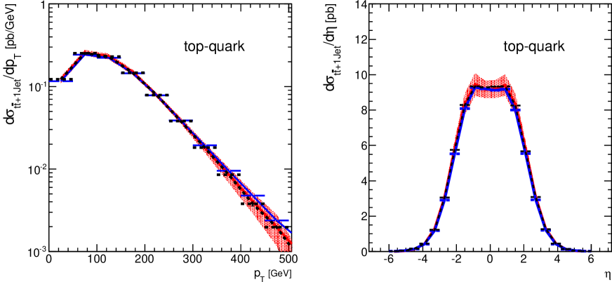
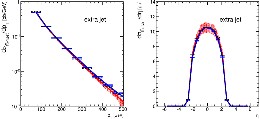
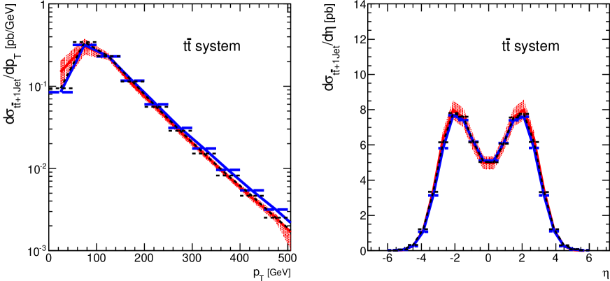
The POWHEG results were obtained in combination with the Pythia 8.150  parton shower. In general the agreement between different approaches is very good. Only at large transverse momentum we observe minor differences. While the fixed-order parton level results agree well with $t\bar{t}+1\textnormal{\normalsize-jet}$@NLO + POWHEG, the results obtained with $t\bar{t}$@NLO + POWHEG are slightly larger. Since the hard emission in $t\bar{t}$@NLO + POWHEG is only treated in LO, this could be a consequence of the missing double real emission processes. In $t\bar{t}$@NLO + POWHEG any additional jet activity beyond the first emission is entirely due to the parton shower which prefers soft and collinear emissions. In the fixed-order $t\bar{t}+1\textnormal{\normalsize-jet}$ calculation and also in the corresponding POWHEG implementation a second hard parton—which may be clustered in a second jet—is included already in the hard matrix elements. The effect of this hard emission can easily explain the reduced average transverse momentum at large $p_{T}$ . In case of the transverse momentum distribution of the $t\bar{t}$ system we observe differences at low $p^{t\bar{t}}_{T}$ between the fixed-order calculation and the two POWHEG implementations. This is not unexpected, because it is precisely the region where the parton shower approach resums logarithmically enhanced corrections to all orders. Due to the additional cut which we have imposed on the light jet this does not occur in the transverse momentum distribution of the light jet.

The various studies presented above show, that the theoretical description of the $t\bar{t}+1\textnormal{\normalsize-jet}$ process at NLO accuracy in QCD is well under control.

2.1 Top-quark mass measurements with $t\bar{t}+1\textnormal{\normalsize-jet}$ events

As shown in Eq. (1), the mass sensitivity of the $t\bar{t}+1\textnormal{\normalsize-jet}$ cross section $\sigma_{t\bar{t}+\textnormal{\scriptsize 1-jet}}$ is very similar to the inclusive $t\bar{t}$ cross section. Therefore, most likely, a measurement of the ‘inclusive’ $t\bar{t}+1\textnormal{\normalsize-jet}$ cross section would not lead to any significant improvement compared to the mass measurements already performed in inclusive top-quark pair production. Instead, we would like to propose an alternative approach.

Since inclusive cross sections are in general difficult to measure, we propose to study normalized differential distributions. Evidently distributions contain more information and may be more sensitive to the mass parameter. Furthermore, due to the normalization many experimental and theoretical uncertainties cancel between numerator and denominator. In order to enhance the mass sensitivity of $t\bar{t}+1\textnormal{\normalsize-jet}$ events we need to focus on kinematical configurations where an enhanced sensitivity can be expected. A natural observable to look at is the (normalized) differential distribution of the $t\bar{t}+1\textnormal{\normalsize-jet}$ cross section with respect to the invariant mass squared $s_{t\bar{t}j}$ of the final state. More precisely we study the dimensionless distribution

$${\cal R}(m_{t}^{\mbox{\scriptsize pole}},\rho_{s})=\frac{1}{\sigma_{t\bar{t}+\textnormal{\scriptsize 1-jet}}}\frac{d\sigma_{t\bar{t}+\textnormal{\scriptsize 1-jet}}}{d\rho_{s}}(m_{t}^{\mbox{\scriptsize pole}},\rho_{s}),$$ (3)

where $\rho_{s}$ is defined as

$$\rho_{s}=\frac{2m_{0}}{\sqrt{s_{t\bar{t}j}}}.$$ (4)

The definition of the variable $\rho_{s}$ is similar to the variable $\rho=2m_{t}/\sqrt{s}$ often used in inclusive top-quark pair production. However, since we want to measure the top-quark mass, $m_{t}$ cannot be used in the definition of $\rho_{s}$. Instead we use a scale $m_{0}$ of the order of the top-quark mass. In the following we set $m_{0}=170$ GeV. Note, that in principle an arbitrary renormalization scheme for the top-quark mass can be chosen. In this article we will restrict the analysis to the pole mass scheme. The conversion from the pole mass scheme to other schemes is feasible albeit technically involved. We leave this issue for future studies.

Figure 2: Comparison between ${\cal R}(m_{t}^{\mbox{\scriptsize pole}},\rho_{s})$ calculated at LO and NLO accuracy for a $m_{t}^{\mbox{\scriptsize pole}}=170$ GeV and using the CT09MC1 and CTEQ6.6 PDF sets, respectively. Below we show the ratio NLO/LO.

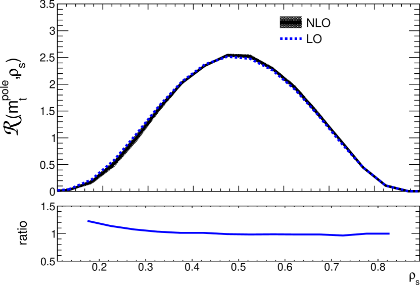
In Fig. 2 we show LO and NLO predictions for the distribution ${\cal R}$ as defined in Eq. (3). LO and NLO distributions are normalized to the respective LO and NLO cross sections. Given that the area under both curves is equal to one the curves need to cross which happens at $\rho_{s}\approx 0.45$. We observe that in the region close to the threshold which corresponds to $\rho_{s}\approx 1$ the LO and NLO predictions agree reasonable well. In Fig. 3 we compare results for different PDF sets.

Figure 3: Predictions for ${\cal R}$ at NLO accuracy using two different PDF sets (CTEQ6.6, MSTW2008nlo) for $m_{t}^{\mbox{\scriptsize pole}}=170$ GeV. For CTEQ6.6 the uncertainty due to scale variation is shown as band. The ratio between both predictions is shown together with the scale uncertainty.

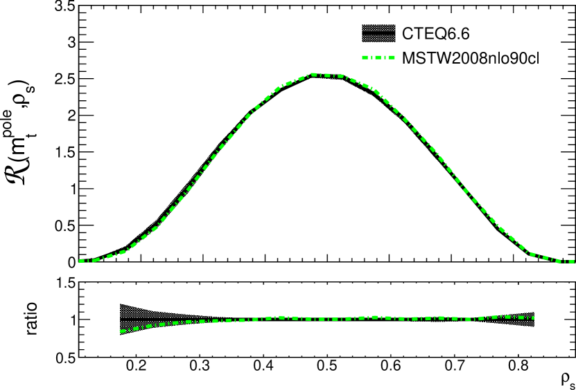
In black we show the default setup where we use the CTEQ6.6 PDF set. In green the result for the MSTW2008NLO set is shown. As a consequence of the normalization the PDF dependence essentially cancels and the curves lie on top of each other. Fig. 3 also shows the uncertainty due to scale variations (black band). Evidently the scale uncertainty is further reduced compared to the unnormalized quantities, since the leading power in the strong coupling constant $\alpha_{s}$ cancels in the ratio. One may argue that in such a situation the scale variation does not provide a sensible method to estimate the effect of uncalculated higher order terms. As a cross check we have compared the naive way to calculate ${\cal R}$ where we just divide the differential distribution by $\sigma_{t\bar{t}+\textnormal{\scriptsize 1-jet}}$ with the expanded version where we perform a strict expansion of ${\cal R}$ in $\alpha_{s}$. We find that both methods lead to roughly the same estimate for the uncertainty. We note that using the running top-quark mass instead of the pole mass could in principle lead to a further reduction of the scale uncertainty.

Figure 4: ${\cal R}(m_{t}^{\mbox{\scriptsize pole}},\rho_{s})$ calculated at NLO accuracy for different masses $m_{t}^{\mbox{\scriptsize pole}}=160,\,170$ and $180$ GeV. For $m_{t}^{\mbox{\scriptsize pole}}=170$ GeV the scale and PDF uncertainties evaluated as discussed in the text are shown. The ratio with respect to the result for $m_{t}^{\mbox{\scriptsize pole}}=170$ GeV is shown in the lower plot.

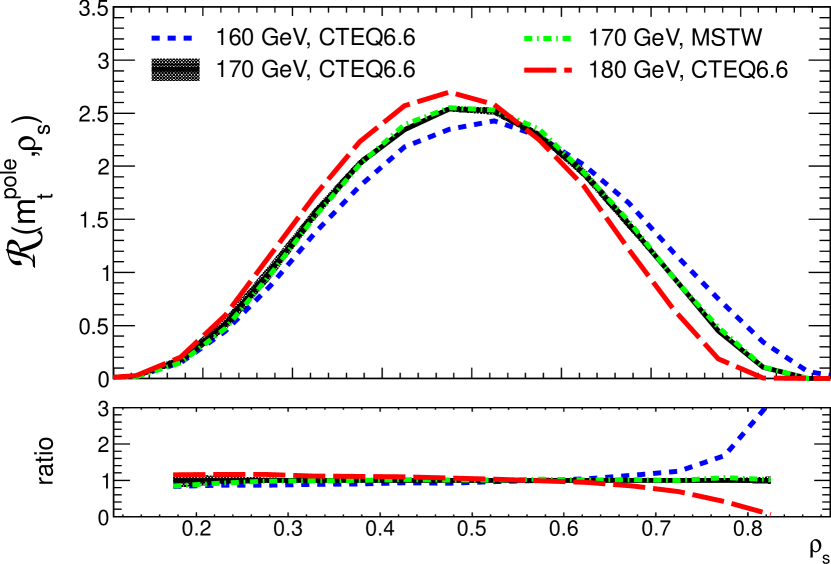
To investigate the sensitivity of the distribution ${\cal R}$ to the top-quark mass we have calculated ${\cal R}$ for $m_{t}^{\mbox{\scriptsize pole}}=160,170,180$ GeV. The result is shown in Fig. 4. As before the three curves need to cross since the area under each curve is normalized to one. The crossing happens slightly below $\rho_{s}\approx 0.6$. At this point the distribution is essentially insensitive to the top-quark mass. For $\rho_{s}\approx 1$ we expect that the production of heavier quark masses is suppressed compared to lighter masses. Indeed the distribution for $m_{t}^{\mbox{\scriptsize pole}}=180$ GeV is below the central curve while the 160 GeV result lies above the result for 170 GeV. In the high energy regime, that is for $\rho_{s}\approx 0$, we expect the opposite to be true due to the normalization. For very large energies we observe that the mass dependence is small as one would naively expect. From Fig. 4 we conclude that a significant mass dependence can be observed for $0.4<\rho_{s}<0.5$ and $0.7<\rho_{s}$. To quantify the sensitivity we studied the quantity

$${\cal S}(\rho_{s})\,=\,$$ (5)

$$\sum_{\Delta=\pm 5-10\textnormal{\scriptsize~{}GeV}}\frac{|{\cal R}(170~{}\textnormal{GeV},\rho_{s})-{\cal R}(170~{}\textnormal{GeV}+\Delta,\rho_{s})|}{2|\Delta|{\cal R}(170~{}\textnormal{GeV},\rho_{s})}\,.$$

Figure 5: The sensitivity ${\cal S}(\rho_{s})$ of ${\cal R}$ with respect to the top-quark mass as defined in Eq. (5).

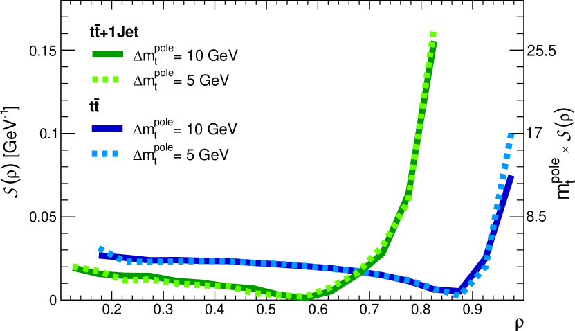
The result for ${\cal S}$ is shown in Fig. 5. For convenience the right $y$-axis shows $m_{t}^{\mbox{\scriptsize pole}}\times{\cal S}$ which is the proportionality factor relating the relative change in the top-quark mass with the relative change in ${\cal R}$:

$$\left|{\Delta{\cal R}\over{\cal R}}\right|\approx\left(m_{t}^{\mbox{\scriptsize pole}}{\cal S}\right)\,\times\,\left|{\Delta m_{t}^{\mbox{\scriptsize pole}}\over m_{t}^{\mbox{\scriptsize pole}}}\right|.$$ (6)

As can be seen in Fig. 5 values up to 25 are reached for $m_{t}^{\mbox{\scriptsize pole}}\times{\cal S}$ at $\rho\approx 0.8$. With other words a one per cent change of the mass translates into a 25 per cent change of the observable ${\cal R}$. The observable is thus five times more sensitive than the inclusive cross section. For comparison, in Fig. 5, we also show the sensitivity in case ${\cal R}$ is defined for the $t\bar{t}$ inclusive final state. (In the $t\bar{t}$ case we use the definition $\rho=2m_{0}/\sqrt{s_{t\bar{t}}}$.) As one can see only in the extreme threshold region—where reliable theoretical predictions are challenging and also experimental uncertainties may become large— a similar sensitivity can be reached. Note that the evaluation of the sensitivity relies on the assumption of a nearly linear top-quark mass dependence. To cross check this assumption we have used two different step sizes in Eq. (5) (5 and 10 GeV). As can be seen from Fig. 5 the two results are in perfect agreement. For a measurement not only the sensitivity is important but also the expected theoretical and experimental uncertainty. For example in the extreme threshold regime a good sensitivity can be expected. However a reliable theoretical prediction in that regime would require to go beyond fixed order perturbation theory to resum threshold effects and soft gluon emission. To estimate the impact of different uncertainties we show in Fig. 6 the quantities

$$\frac{\Delta{\cal R}_{\mu}/{\cal R}(170~{}\textnormal{GeV},\rho_{s})}{{\cal S}(\rho_{s})}\mbox{ and }\frac{\Delta{\cal R}_{\textnormal{\scriptsize PDF}}/{\cal R}(170~{}\textnormal{GeV},\rho_{s})}{{\cal S}(\rho_{s})}$$ (7)

where $\Delta{\cal R}_{\mu}$ and $\Delta{\cal R}_{\textnormal{\scriptsize PDF}}$ are the scale and PDF uncertainties of ${\cal R}(172.5~{}\textnormal{GeV},\rho_{s})$. We do not show the region around $\rho_{s}\approx 0.6$ because of the vanishing sensitivity to the top-quark mass. Fig. 6 shows that the main source of uncertainty comes from the scale variation while the impact of the PDF uncertainties is much smaller.

Figure 6: Expected impact of scale (magenta line) and PDF (blue dashed line) uncertainties on the measured top-quark mass value. The region where ${\cal R}$ is essentially insensitive to the top-quark mass is not shown.

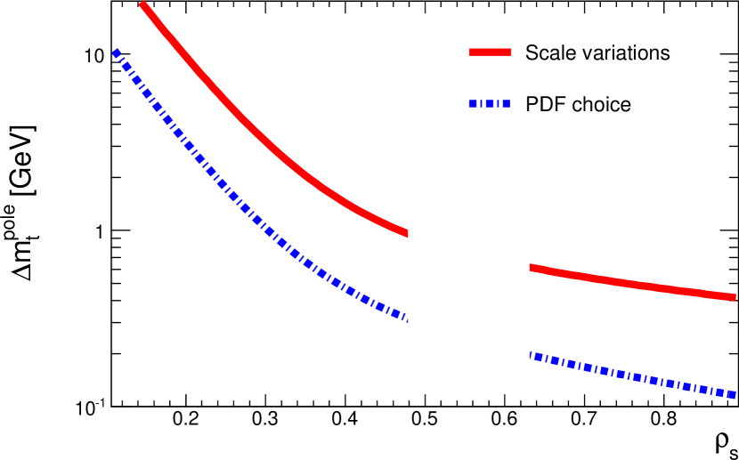
From Fig. 6 we conclude that for $\rho_{s}>0.65$ the dominant uncertainty is still below 1 GeV. The low $\rho_{s}$ region, where ${\cal R}$ loses its sensitivity to the top-quark mass, could be used as control region for the experimental reconstruction of ${\cal R}$.

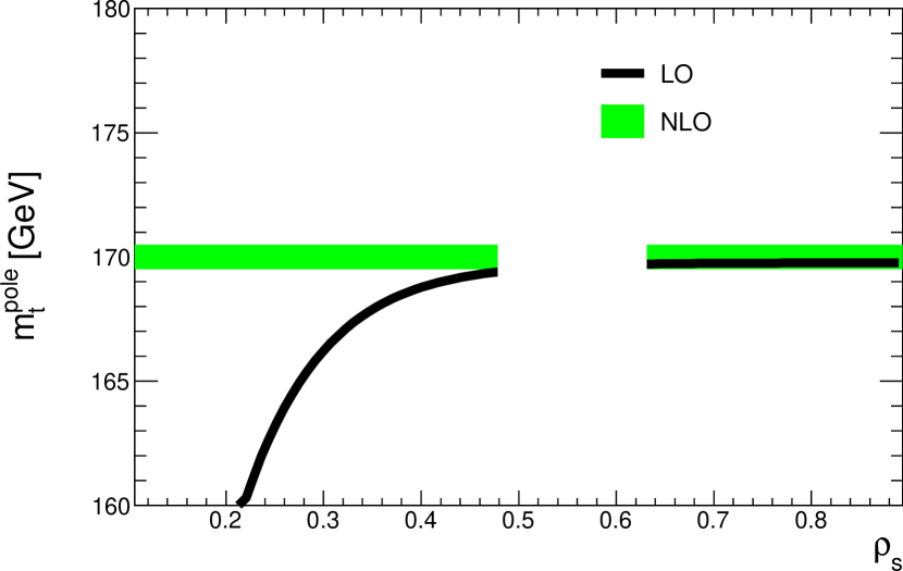
To investigate further the impact of higher order corrections and the effect of the parton shower we have compared the predictions for ${\cal R}(m_{t}^{\mbox{\scriptsize pole}},\rho_{s})$ using different approximations: LO, $t\bar{t}$@NLO + POWHEG Frixione:2007nw , $t\bar{t}+1\textnormal{\normalsize-jet}$ @NLO + POWHEG Alioli:2011as . In Figs. 7 and 8 we show the comparison as result of a toy experiment. We first calculate ${\cal R}$ in NLO accuracy at parton level. In a next step we compare with the different approximations mentioned before and ask what top-quark mass we would measure with a given approximation to explain the ${\cal R}$ result calculated in NLO accuracy. In Fig. 7 the comparison with the LO calculation is shown. As input value we used $m_{t}^{\mbox{\scriptsize pole}}=170~{}\textnormal{GeV}$ in the NLO calculation. The thickness of the band denotes a $\pm 0.5$ GeV uncertainty. In the threshold region the LO result is below the NLO curve (compare Fig. 2). As a consequence we would fit a smaller top-quark mass to account for the deficit in that region. The shift in the threshold region is about 2–3 GeV. In the large energy regime the NLO result is below (see Fig. 2) the LO result. Since in this regime the mass effect works in opposite direction the fit using LO predictions would again yield a smaller top-quark mass. However the NLO corrections are much larger compared to the threshold region. As a consequence the shift in the top-quark mass is more significant.
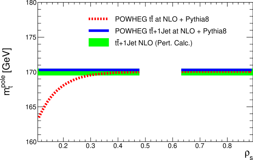
In Fig. 8 the same analysis is shown for $t\bar{t}$@NLO + POWHEG and $t\bar{t}+1\textnormal{\normalsize-jet}$ @NLO + POWHEG. Since the various predictions agree very well with each other we find agreement of the different approximations within  500 MeV for the extracted top-quark mass.

Figure 7: The top-quark mass $m_{t}^{\mbox{\scriptsize pole}}$ as obtained from a LO fit to ${\cal R}$ calculated in NLO accuracy (black line). The input value of $m_{t}^{\mbox{\scriptsize pole}}=170$ GeV together with a variation of $\pm 0.5$ GeV is shown as green band.

Figure 8: Similar to Fig. 7 however $t\bar{t}$@NLO + POWHEG and $t\bar{t}+\mbox{1-jet}+X$@NLO + POWHEG are used to fit the top-quark mass.

From the above findings we conclude that ${\cal R}$ shows a good sensitivity to the top-quark mass while at the same time theory uncertainties lead to small uncertainties in the reconstructed mass value. We are thus lead to the conclusion that from the theoretical perspective ${\cal R}$ provides an interesting alternative to existing methods for top-quark mass measurements.

3 Experimental viability study

Evidently for a true measurement the nice theoretical properties of ${\cal R}$ discussed in the previous section are not sufficient to conclude that a measurement with a certain precision can be achieved. In this section additional properties of the ${\cal R}$ distribution which may affect the experimental analysis are investigated. For a realistic study we use only stable particles in the final state originating from typical $t\bar{t}+\mbox{1-jet}+X$ events as produced in proton-proton interactions at 7 TeV center-of-mass energy. In particular the top-quark decay and hadronization are taken into account leading to complicated event topologies similar to those reconstructed in real experiments. In the Monte Carlos studies we use only publicly available tools and do not make any reference to a particular LHC experiment. Since detector effects are to a large extent generic we believe however that this should be sufficient to assess the dominant experimental uncertainties. The sources of uncertainties included in this study are those which usually have a high impact on similar multi-jet topologies. They are related to: top-quark identification, jet identification and jet-jet invariant mass reconstruction. The results obtained are intended to qualitatively illustrate the reach of the method. A real experimental determination will necessarily need a more detailed and careful detector analysis.

In the SM the top quark decays almost exclusively into a $W$ boson and a $b$ quark and consequently a top-quark pair will give rise to two $b$ quarks and two $W$ bosons that (each one of them) will further decay into two quarks or into a lepton ($\ell$) and a neutrino ($\nu$). This study only considers the so called semi-leptonic decay channel which assumes that one of the two $W$ boson decays leptonically whereas the remaining $W$ boson decays hadronically. All quarks produced will later evolve into the hadronization and decay processes until stable particles are produced. This semi-leptonic channel has a very good balance between efficient identification and event rate since roughly $8/27$ of all top-quark pair events decay semi-leptonically (as usual we exclude the tau decay from the leptonic decays). These final state configurations can be identified by the presence of one high-$p_{T}$ lepton (in our case only electrons and muons are considered), high missing transverse energy because of the presence of the neutrino, two jets originating from the $b$ quarks and at least two additional jets.

Unless it is stated differently the observable ${\cal R}$ has been calculated using event samples simulated with $t\bar{t}+1\textnormal{\normalsize-jet}$ @NLO + POWHEG matched with Pythia as the parton shower generator and the fragmentation model. Jets are defined using the FastJet package Cacciari:2011ma and the anti-kt algorithm Cacciari:2008gp with R=0.4 consistent with the perturbative study in the previous section. Selected events are required to fulfill the following conditions:

1. only one lepton ($\ell=e,\mu$) with $p_{T}>$ 25 GeV and $|\eta|<$ 2.5;

2. missing transverse energy larger $30$ GeV to account for the presence of a neutrino;

3. a large transverse mass of the leptonic system $M^{W}_{T}>35$ GeV produced by the W boson decay;

4. at least 3 jets with $|\eta|<2.5$, one of them with $p_{T}>50$ GeV and the other two with $p_{T}>25$ GeV;

5. two additional identified b-jets.

The jet with the highest energy is associated with the additional jet emitted in the hard scattering and the other two are assumed to originate from the $W$ boson decaying hadronically.

In addition to these conditions other constraints based on the event topology are applied. The invariant mass of the two non $b$-jets are required to be compatible with the mass of the $W$ boson within 20% and the two reconstructed top-jet systems are required to have similar masses within a range of precision also around 20%. The missing energy has to be compatible with a neutrino which, together with the identified lepton can both be attributed to originate from the decay of the $W$ boson. These conditions guarantee a good reconstruction of the jet energies though better tunings or more optimized methods are available for this purpose. However more involved methods would imply using detailed detector specific tools which are beyond the scope of this exercise. It should be noticed that it is only at this stage when the correct jet association is imposed to test the hypothesis that the event originates from two top quarks. In fact the quantity $\rho_{s}$ considered depends on the invariant mass of all jets and fermions and is therefore independent of misidentified jet associations.

After this selection the ${\cal R}$ distribution has been successfully reconstructed and the impact of the following effects has been studied:

• the event generator and fragmentation model: POWHEG with Pythia versus MC@NLO Frixione:2002ik with Herwig Corcella:2000bw ; Corcella:2002jc ,

• backgrounds, mainly QCD, single top and $W$+jets,

• the impact of a wrongly reconstructed jet energy,

• the unfolding procedure to correct the ${\cal R}$ distribution to the perturbative partonic level,

• the statistical error depending on the collected luminosity,

• different modeling of color reconnection.

The comparison between POWHEG interfaced with Pythia and MC@NLO interfaced with Herwig shows that the reconstructed ${\cal R}$ distribution is very stable independent of the choice of the parton shower generator and the fragmentation model which are selected in the simulation. The value of $m_{t}^{\mbox{\scriptsize pole}}$ which is obtained using one or the other model is found to remain stable within $0.20\pm 0.20$ GeV for the high range of $\rho_{s}$.

The presence of a high $p_{T}$ lepton (cut 1) and missing transverse energy (cut 2) reduces the QCD background. The $W$+jets and single top contamination is reduced by applying the cuts 3,4 and 5. The final background is thus expected to be well understood and can be kept low ($5-10$%) allowing for an easy subtraction with very small impact on the final uncertainties.

Figure 9: Impact of an uncertainty of $\pm$3% in the jet energy scale.

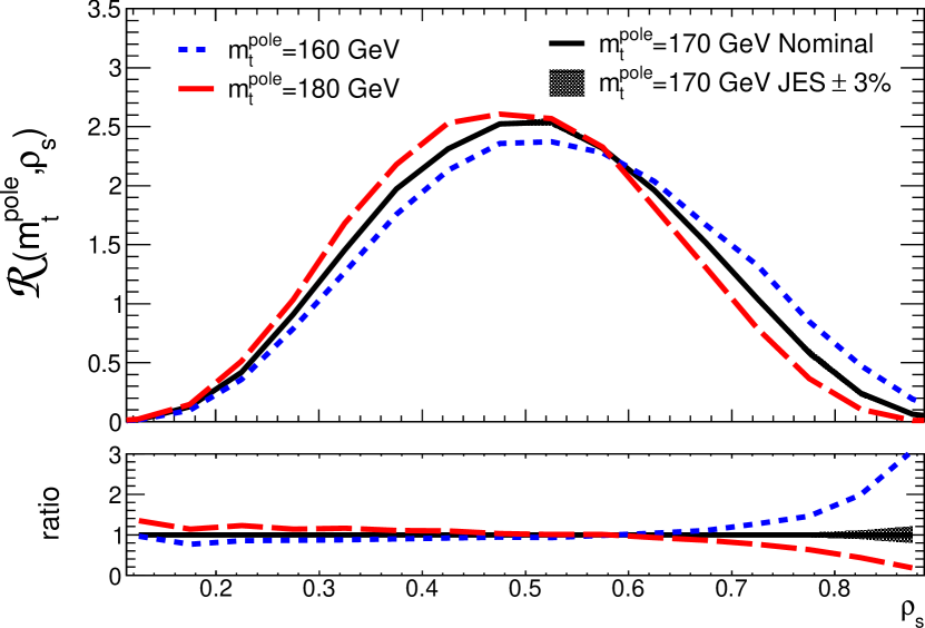
The measured jet energy in the experiments can be distorted due to different detection effects, such as, response of the calorimeters to different particles, non-linearity responses of the detectors to the particle energies, un-instrumented regions of the detector, energy radiated outside the jet clustering algorithm, etc. The uncertainty related to this kind of effects is often attributed to the jet energy scale (JES). To estimate these effects the energy of the jets has been changed by $3\%$ up and $3\%$ down before the construction of ${\cal R}$. The result is shown in Fig. 9. The black band illustrates the uncertainty changing the JES scale by $\pm$3%. As reference we show also the result for ${\cal R}$ using 160 and 180 GeV as input for the top-quark mass. Applying the topological constraints described previously, the impact of this change to the top-quark mass measured using ${\cal R}$ has been computed to be around $0.8-1.0$ GeV. A better compromise between efficiency and resolution is possible though it would imply tools which are detector specific.

Figure 10: Mass independence of the unfolding procedure.

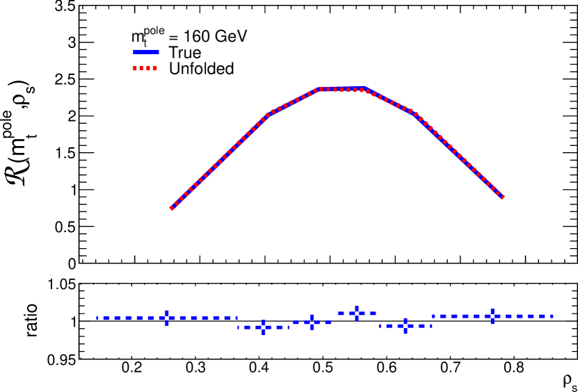
It is important to realize that the observable proposed in this article allows to unfold the data and reproduce the original ${\cal R}$ distribution at parton level—without relying on a preset mass value which would introduce what is often called the Monte Carlo mass. A method based on the shape of the distribution has been developed for this purpose. In Fig. 10 we illustrate the result of this procedure. The unfolding procedure has been constructed using Monte Carlo simulations for $m_{t}^{\mbox{\scriptsize pole}}=170$ GeV. We have than applied the method to an event sample generated for $m_{t}^{\mbox{\scriptsize pole}}=160$ GeV. In Fig. 10 we compare the result of the unfolding procedure with the Monte Carlo truth information. As one can see the two curves lie on top of each other. The uncertainty related to the unfolding is below one per cent. The results thus show that a mass independent unfolding is indeed possible in the region from $m_{t}^{\mbox{\scriptsize pole}}=160$ GeV to $m_{t}^{\mbox{\scriptsize pole}}=180$ GeV. Due to the limited statistics used in this study the previous statement has an associated uncertainty of $\sim$0.3 GeV. The robustness of the method is thus reinforced by this result as it shows that the correction procedure is not sensitive to the different topological and phase-space configurations arising from the possible different top-quark mass values. The influence of the minimum gluon-jet $p_{T}$ has also been studied in the range 30 GeV $\leq p_{T}\leq$ 60 GeV in this context. Again within the limited statistics we find that the correction factors are stable at the level of 0.7%.

To evaluate the statistical error we assume 5 fb^-1 collected luminosity and a final efficiency of 1% with respect to the original $t\bar{t}+1\textnormal{\normalsize-jet}$ cross section as shown in table 1. The expected statistical error is around 1.4 GeV when integrating the high sensitivity region $\rho_{s}>0.65$ for this amount of collected luminosity.

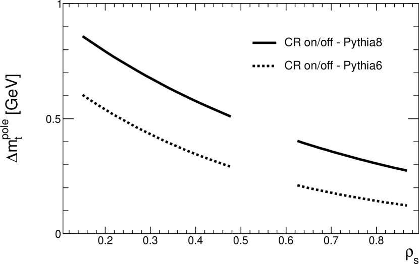
As a last major uncertainty we have investigated the effect of color reconnection. In the top-quark mass measurement via kinematical reconstruction, the color reconnection directly affects the location of the peak of the reconstructed distribution. As a consequence one may expect effects of the order of 100 MeV. Indeed in Ref. Skands:2007zg it is argued that an uncertainty of about 500 MeV due to color reconnection can be expected. In the approach advocated here we do not expect that color reconnection plays an important role since the observable itself does not rely on a precise momentum reconstruction. The momenta enter only through the jet algorithm which determines whether an event passes the jet selection cuts. We expect only a very weak effect of color reconnection on the jet algorithm. Apart from this, color reconnection could in principle also affect the determination of $s_{t\bar{t}j}$, however since $s_{t\bar{t}j}$ is an inclusive quantity we do not expect a major effect here. Furthermore an incorrect determination of $s_{t\bar{t}j}$ would only affect events at the bin boundaries and is not unlikely that migrations at the left border and the right border will compensate to a large extent. To study the impact of color reconnection two different approaches have been investigated using the Pythia versions Pythia6 and Pythia8 Sjostrand:2006za which consider two distinct color reconnection schemes. In the Pythia8 color reconnection is assumed to happen before the top quarks decay while in Pythia6, the color reconnection process is performed after the top and $W$ decays. The main issue to consider is the top lifetime and $W$ widths, and its relation with the time which it takes the reconnection process to occur. To assess the impact of color reconnection on ${\cal R}$ we used both Pythia6 and Pythia8 and compared the situation of using color reconnection in the respective default setup to the situation where color reconnection is completely switched off. The related uncertainty of the extracted top-quark mass is shown in Fig. 11. Evidently the aforementioned procedure gives a rather extreme estimate of the uncertainty. We believe that the uncertainy given here is much more conservative compared to what has been done in Ref. Skands:2007zg where essentially only the impact of different tunes has been investigated. As a consequence the true uncertainty could be significantly smaller compared to what is shown in Fig. 11. In any case we conclude that even in the worst case the uncertainy is below 400 MeV using reasonable values for $\rho_{s}$.

Figure 11: Impact of color reconnection on the top-quark mass determination using ${\cal R}$. The solid line shows the effect using Pythia8 and switching color reconnection on and off. The dashed line shows the corresponding result using Pythia6.

The above mentioned results prove the experimental viability and the potential of the method. A real analysis using data and detector specific tools is needed to understand the exact value of the uncertainties affecting the determination of $m_{t}^{\mbox{\scriptsize pole}}$ but we can estimate that a total error around of 1 GeV or lower is achievable.

4 Conclusions

In this article we propose a new method for top-quark mass measurements at hadron colliders and in particular at the LHC. In detail the differential distribution of the $t\bar{t}+1\textnormal{\normalsize-jet}$ cross section with respect to $m_{0}/\sqrt{s_{t\bar{t}j}}$ is investigated. We have shown that theoretical predictions for this quantity are well under control and that the observable shows a good sensitivity to the top-quark mass. Uncertainties related to uncalculated higher order corrections or uncertainties in the parton distribution functions are expected to affect the mass measurement by less than 1 GeV. In a study of the experimental viability we have addressed all major uncertainties without using a specific detector set-up. Again we find that the impact on the top-quark mass measurement is below 1 GeV. Since in the analysis presented here the renormalization scheme of the top-quark mass is uniquely defined we believe that the method nicely complements existing approaches.

5 APPENDIX

Table 3: Similar to Tab. 1 but for a $p_{T}$ cut of 25 GeV in difference to 50 GeV used in Tab. 1.

	$\sigma_{t\bar{t}+1-\textrm{\scriptsize jet}}$ (pb)
	$p_{T}(jet)>25\,\textrm{GeV},\,|\eta(jet)|<2.5$
$m_{t}^{\mbox{\scriptsize pole}}$ [GeV]	LO	NLO
$170$	$91.827(8)^{+53}_{-31}$	$77.7(1)^{-1}_{-9}$
$172.5$	$85.39(1)^{+50}_{-29}$	$72.43(6)^{-2}_{-9}$

Table 4: Similar to Tab. 2 but for $m_{t}^{\mbox{\scriptsize pole}}=172.5$ GeV.

$\sigma_{t\bar{t}+1-\textrm{\scriptsize jet}}$ [pb]
$t\bar{t}$	without addtional PS	47.2(1)
NLO	PS by Pythia8	43,2(5)
$t\bar{t}+\mbox{1-jet}$	without addtional PS	44.9(5)
NLO	PS by Pythia8	43,0(5)

References

- (1) T. Aaltonen, et al., Phys.Rev.D (2012)
- (2) V.M. Abazov, et al., Phys.Lett. B703, 422 (2011). DOI 10.1016/j.physletb.2011.08.015
- (3) J. Beringer, et al., Phys.Rev. D86, 010001 (2012). DOI 10.1103/PhysRevD.86.010001
- (4) G. Aad, et al., Phys.Lett. B716, 1 (2012). DOI 10.1016/j.physletb.2012.08.020
- (5) S. Chatrchyan, et al., Phys.Lett. B716, 30 (2012). DOI 10.1016/j.physletb.2012.08.021
- (6) S. Heinemeyer, W. Hollik, D. Stockinger, A. Weber, G. Weiglein, JHEP 0608, 052 (2006). DOI 10.1088/1126-6708/2006/08/052
- (7) G. Degrassi, S. Di Vita, J. Elias-Miro, J.R. Espinosa, G.F. Giudice, et al., JHEP 1208, 098 (2012). DOI 10.1007/JHEP08(2012)098
- (8) S. Alekhin, A. Djouadi, S. Moch, Phys.Lett. B716, 214 (2012). DOI 10.1016/j.physletb.2012.08.024
- (9) M.S. Bilenky, S. Caberera, J. Fuster, S. Marti, G. Rodrigo, et al., Phys.Rev. D60, 114006 (1999). DOI 10.1103/PhysRevD.60.114006
- (10) U. Langenfeld, S. Moch, P. Uwer, Phys.Rev. D80, 054009 (2009). DOI 10.1103/PhysRevD.80.054009
- (11) M. Aliev, H. Lacker, U. Langenfeld, S. Moch, P. Uwer, et al., Comput.Phys.Commun. 182, 1034 (2011). DOI 10.1016/j.cpc.2010.12.040
- (12) S. Dittmaier, P. Uwer, S. Weinzierl, Phys.Rev.Lett. 98, 262002 (2007). DOI 10.1103/PhysRevLett.98.262002
- (13) S. Dittmaier, P. Uwer, S. Weinzierl, Eur.Phys.J. C59, 625 (2009). DOI 10.1140/epjc/s10052-008-0816-y
- (14) S. Alioli, S.O. Moch, P. Uwer, JHEP 1201, 137 (2012). DOI 10.1007/JHEP01(2012)137
- (15) S.D. Ellis, D.E. Soper, Phys.Rev. D48, 3160 (1993). DOI 10.1103/PhysRevD.48.3160
- (16) M. Cacciari, G.P. Salam, G. Soyez, JHEP 0804, 063 (2008). DOI 10.1088/1126-6708/2008/04/063
- (17) M. Cacciari, G.P. Salam, G. Soyez, Eur.Phys.J. C72, 1896 (2012). DOI 10.1140/epjc/s10052-012-1896-2
- (18) P.M. Nadolsky, et al., Phys. Rev. D78, 013004 (2008). DOI 10.1103/PhysRevD.78.013004
- (19) H.L. Lai, J. Huston, S. Mrenna, P. Nadolsky, D. Stump, et al., JHEP 1004, 035 (2010). DOI 10.1007/JHEP04(2010)035
- (20) A. Martin, W. Stirling, R. Thorne, G. Watt, Eur.Phys.J. C63, 189 (2009). DOI 10.1140/epjc/s10052-009-1072-5
- (21) S. Alekhin, J. Blumlein, S. Moch, Phys.Rev. D86, 054009 (2012). DOI 10.1103/PhysRevD.86.054009
- (22) S. Alioli, P. Nason, C. Oleari, E. Re, JHEP 1006, 043 (2010). DOI 10.1007/JHEP06(2010)043
- (23) S. Frixione, P. Nason, G. Ridolfi, JHEP 0709, 126 (2007). DOI 10.1088/1126-6708/2007/09/126
- (24) A. Kardos, C. Papadopoulos, Z. Trocsanyi, Phys.Lett. B705, 76 (2011). DOI 10.1016/j.physletb.2011.09.080
- (25) T. Sjöstrand, S. Mrenna, P.Z. Skands, Comput. Phys. Commun. 178, 852 (2008). DOI 10.1016/j.cpc.2008.01.036
- (26) S. Frixione, B.R. Webber, JHEP 0206, 029 (2002)
- (27) G. Corcella, I. Knowles, G. Marchesini, S. Moretti, K. Odagiri, et al., JHEP 0101, 010 (2001)
- (28) G. Corcella, I. Knowles, G. Marchesini, S. Moretti, K. Odagiri, et al., (2002)
- (29) P.Z. Skands, D. Wicke, Eur.Phys.J. C52, 133 (2007). DOI 10.1140/epjc/s10052-007-0352-1
- (30) T. Sjostrand, S. Mrenna, P.Z. Skands, JHEP 0605, 026 (2006). DOI 10.1088/1126-6708/2006/05/026