Unconditionally optimal error analysis of fully discrete Galerkin methods for general nonlinear parabolic equations

Abstract

The paper focuses on unconditionally optimal error analysis of the fully discrete Galerkin finite element methods for a general nonlinear parabolic system in $\mathbb{R}^{d}$ with $d=2,3$. In terms of a corresponding time-discrete system of PDEs as proposed in [22], we split the error function into two parts, one from the temporal discretization and one the spatial discretization. We prove that the latter is $\tau$-independent and the numerical solution is bounded in the $L^{\infty}$ and $W^{1,\infty}$ norms by the inverse inequalities. With the boundedness of the numerical solution, optimal error estimates can be obtained unconditionally in a routine way. Several numerical examples in two and three dimensional spaces are given to support our theoretical analysis.

Key words: Optimal error estimates, unconditional stability, Galerkin, nonlinear parabolic system

1 Introduction

There are several numerical approximations schemes in the time direction for the numerical solution of nonlinear parabolic equations (systems). Linearized (semi)-implicit schemes are the most popular ones since, at each time step, the schemes only require the solution of a linear system. However, time-step size restriction condition is always a key issue in analysis and computation. For many nonlinear parabolic systems, error analysis of finite element methods (or finite difference method) with linearized semi-implicit schemes in the time direction often requires certain time-step conditions. See [1, 18, 20, 25, 29] for the Navier-Stokes equations, [14, 40] for the nonlinear Joule heating problems, [11, 13, 16, 19, 34] for flows in porous media, [7, 15, 35] for viscoelastic fluid flow, [26, 39] for the KdV equations, [8, 27] for the Ginzburg-Landau equations, [3, 5, 33, 42] for the nonlinear Schrödinger equations and [10, 17, 37] for some other equations. Such time-step size restrictions may result in the use of an unnecessarily small time-step size and extremely time-consuming in practical computations. To study the error estimate of linearized (semi)-implicit schemes, the boundedness of numerical solution (or error function) in the $L^{\infty}$ norm or a stronger norm is often required. If a priori estimate for the numerical solution in such a norm cannot be provided, one may employ the induction method with an inverse inequality to bound the numerical solution, such as

$$\|U_{h}^{n}-R_{h}u^{n}\|_{L^{\infty}}\leq Ch^{-d/2}\|U_{h}^{n}-R_{h}u^{n}\|_{L^{2}}\leq Ch^{-d/2}(\tau^{m}+h^{r+1}),$$ (1.1)

where $U_{h}^{n}$ is the finite element solution, $u$ is the exact solution and $R_{h}$ is certain projection operator. A time-step size restriction arises immediately from the above inequality, particularly for problems in three dimensional spaces. Most previous works follow this idea. A new approach for unconditionally optimal error analysis of a linearized Galerkin FEM was pesented in our recent work [22], also see [24], where the error function is split into two parts, the spatially discrete error and the temporally discrete error,

$$\|u^{n}-U_{h}^{n}\|\leq\|u^{n}-U^{n}\|+\|U^{n}-U_{h}^{n}\|,$$ (1.2)

where $U^{n}$ is the solution of a corresponding time-discrete parabolic equations (or elliptic equations). Optimal estimates for the second term can be obtained unconditionally in a traditional way if suitable regularity of the solution of the time-discrete system can be proved. More recently, unconditionally optimal error estimates were established for a nonlinear equation from incompressible miscible flow in porous media. In [22, 23], analysis waw given only for a linear FEM and a low-order Galerkin-mixed FEM, respectively.

In this paper, we consider a general nonlinear parabolic equation (or system)

$$\frac{\partial u}{\partial t}-\nabla\cdot(\sigma(u)\nabla u)=g(u,\nabla u,x,t)$$ (1.3)

in a bounded and smooth domain $\Omega$ in $\mathbb{R}^{d}$ ($d=2$ or $3$) with the boundary condition

$$\begin{array}[]{ll}u=0{}{}&\mbox{on}~{}~{}\partial\Omega\end{array}$$ (1.5)

and the initial condition

$$\begin{array}[]{ll}u(x,0)=u_{0}(x){}{}&\mbox{for}~{}~{}x\in\Omega,\end{array}$$ (1.7)

where $g\in C^{2}(\mathbb{R})$ is a general nonlinear source. The general equation is of stronger nonlinearity than those in [22, 23] and many physical equations are included. We apply linearized backward Euler Galerkin method with $r$-order finite element approximation ($r\geq 1$) for the general nonlinear system. We focus our attention on the unconditional convergence (stability) and optimal error estimates of the linearized Galerkin FEMs. A key to our analysis is the a priori estimate of the numerical solution. We apply the splitting technique proposed in [22, 23] to bound the numerical solution $U_{h}^{n}$ in $L^{\infty}$-norm and $W^{1,\infty}$-norm, such as

$$\|U_{h}^{n}\|_{W^{1,\infty}} \leq\|R_{h}U^{n}\|_{W^{1,\infty}}+\|U_{h}^{n}-R_{h}U^{n}\|_{W^{1,\infty}}$$

$$\leq\|R_{h}U^{n}\|_{W^{1,\infty}}+Ch^{-d/2}\|U_{h}^{n}-R_{h}U^{n}\|_{H^{1}}$$

$$\leq C+Ch^{-d/2}h^{k}$$ (1.8)

where $k>d/2$. Then with the boundedness of $\|U_{h}^{n}\|_{W^{1,\infty}}$, optimal error estimates can be easily established unconditionally in the routine way of FEM error analysis.

The paper is organized as follows. In Section 2, we present linearized backward Euler Galerkin FEMs for the general nonlinear parabolic equations (1.3)-(1.7) and introduce our notations. In Section 3, we prove the boundedness of the numerical solution in the $W^{1,\infty}$ norm in terms of a corresponding time-discrete system, in which a rigorous analysis on the regularity of the solution to the time-discrete PDEs is given. Due to the boundedness of the numerical solution in the $W^{1,\infty}$ norm, we present unconditionally optimal error estimates in Section 4 in a simple and routine way. Numerical examples in two and three-dimensional spaces are presented in Section 5. Numerical results confirm our theoretical analysis and show that no time-step condition is needed.

2 Fully discrete Galerkin FEMs

Let $\pi_{h}$ be a regular division of $\Omega$ into triangles $T_{j}$, $j=1,\cdots,M$, in $\mathbb{R}^{2}$ or tetrahedras in $\mathbb{R}^{3}$, and let $h=\max_{1\leq j\leq M}\{\mbox{diam}\,T_{j}\}$ denote the mesh size. For a triangle $T_{j}$ with two corners (or a tetrahedra with three corners) on the boundary, we let $\widetilde{T}_{j}$ denote the triangle with one curved side (or a tetrahedra with one curved face). For an interior triangle, we simply set $\widetilde{T}_{j}$ as $T_{j}$ itself. Finite element spaces on $\{\widetilde{T}_{j}\}$ have been well defined, $e.g.$, see [32, 41]. For a given triangular (or tetrahedral) division of $\Omega$, we define the finite element space

$$\widehat{V}_{h}=\{v_{h}\in C(\overline{\Omega}_{h}):v_{h}|_{T_{j}}\mbox{~{}is~{}a~{}polynomial of degree $r$ and $v_{h}=0$ on $\partial\Omega_{h}$}\}$$

so that $\widehat{V}_{h}$ is a subspace of $H^{1}_{0}(\Omega_{h})$. Let $G:\Omega_{h}\rightarrow\Omega$ be a coordinate transformation such that both $G$ and $G^{-1}$ are Lipschitz continuous and, for each triangle $T_{j}$, $G$ maps $T_{j}$ one-to-one onto $\widetilde{T}_{j}$ [41]. We define an operator ${\cal G}:L^{2}(\Omega_{h})\rightarrow L^{2}(\Omega)$ by ${\cal G}v(x)=v(G^{-1}(x))$ for $x\in\Omega$. Then we set

$$V_{h}=\{{\cal G}v_{h}:v_{h}\in\widehat{V}_{h}\}.$$

Easy to see that $V_{h}$ is a finite element subspace of $H^{1}_{0}(\Omega)$ and

$$\|w-\Pi_{h}w\|_{L^{p}}\leq C\|w\|_{W^{r+1,p}(\Omega)}h^{r+1},\quad\mbox{for}~{}r\geq 1,~{}2\leq p\leq\infty,$$

where $\Pi_{h}={\cal G}\widehat{\Pi}_{h}{\cal G}^{-1}$ and $\widehat{\Pi}_{h}:C_{0}(\overline{\Omega}_{h})\rightarrow\widehat{V}_{h}$ is the Lagrangian interpolation operator of degree $r$.

Let $0=t_{0}<t_{1}<\cdots<t_{N}=T$ be a uniform partition of the time interval $[0,T]$ with $t_{n}=n\tau$ and let $u^{n}=u(x,t_{n})$ for $n=0,1,\cdots,N$. For a sequence of functions $\{f^{n}\}_{n=0}^{N}$, we define

$$D_{\tau}f^{n+1}=\frac{f^{n+1}-f^{n}}{\tau},\quad\mbox{for $n=0,1,\cdots,N-1$.}$$ (2.1)

A simple linearized backward Euler Galerkin method for the problem (1.3)-(1.7) is to seek $U^{n+1}_{h}\in V_{h}$, $0\leq n\leq N-1$, such that

$$\big{(}D_{\tau}U^{n+1}_{h},v\big{)}+\big{(}\sigma(U^{n}_{h})\nabla U^{n+1}_{h},\nabla v\big{)}=\big{(}g(U^{n}_{h},\nabla U^{n}_{h},x,t),v\big{)}$$ (2.2)

for any $v\in V_{h}$, with the initial condition $U^{0}_{h}=\Pi_{h}u_{0}$ for $r\geq 2$ and $U^{0}_{h}=R_{h}^{1}u_{0}$ for $r=1$, where $R_{h}^{1}$ is a projection operator defined in Section 3.2.

With a linear approximation to the nonlinear source term, an alternative linearized scheme is defined by

$$\big{(}D_{\tau}U^{n+1}_{h},v\big{)}+\big{(}\sigma(U^{n}_{h})\nabla U^{n+1}_{h},\nabla v\big{)}=\big{(}g_{0}^{n},v\big{)}+\big{(}g_{1}^{n}U^{n+1}_{h},v\big{)}+\big{(}g_{2}^{n}\cdot\nabla U^{n+1}_{h},v\big{)},\quad\forall~{}v\in V_{h},$$

where $g_{0}^{n}=g(U^{n}_{h},\nabla U^{n}_{h},x,t)$, $g_{1}^{n}=\nabla_{1}g(U^{n}_{h},\nabla U^{n}_{h},x,t)$ and $g_{2}^{n}=\nabla_{2}g(U^{n}_{h},\nabla U^{n}_{h},x,t)$, with $\nabla_{1}g$ and $\nabla_{2}g$ denoting the gradient of $g$ with respect to the components $U$ and $\nabla U$, respectively. The corresponding linearized Crank-Nicolson schemes can be defined similarly with classical extrapolations [12].

In this paper, we only focus our attention on the linearized scheme (2.2). The analysis presented in this paper can be extended to the second linearized scheme and many other schemes. We assume that $g\in C^{2}(\mathbb{R}\times\mathbb{R}^{d}\times\overline{\Omega}\times[0,T])$ and $\sigma\in C^{2}(\mathbb{R})$ satisfies the weak ellipticity condition

$$\sigma(s)>0\quad\mbox{for}~{}~{}s\in\mathbb{R}.$$ (2.3)

3 Boundedness of the numerical solution

In this section, we assume that the solution to the problem (1.3)-(1.5) exists and satisfies that

$$\|u\|_{L^{\infty}((0,T);H^{3})}+\|\partial_{t}u\|_{L^{\infty}((0,T);L^{2})}+\|\partial_{t}u\|_{L^{2}((0,T);H^{2})}+\|\partial_{tt}u\|_{L^{2}((0,T);L^{2})}\leq M,$$ (3.1)

for some positive constant $M$, and we prove the following theorem.

Theorem 3.1

Suppose that the system (1.3)-(1.7) has a unique solution $u$ satisfying the regularity condition (3.1). Then there exist positive constants $C$ and $h_{0}$, independent of $n$ and $h$, such that the finite element system (2.2) admits a unique solution $\{U^{n}_{h}\}_{n=1}^{N}$ when $h<h_{0}$, and

$$\|U_{h}^{n}\|_{L^{\infty}}+\|\nabla U_{h}^{n}\|_{L^{\infty}}\leq C.$$ (3.2)

To prove Theorem 3.1, we introduce a corresponding time-discrete equation as proposed in [22, 23]:

$$D_{\tau}U^{n+1}-\nabla\cdot(\sigma(U^{n})\nabla U^{n+1})=g(U^{n},\nabla U^{n},x,t_{n}),$$ (3.3)

with the boundary condition $U^{n+1}=0$ on $\partial\Omega$ and the initial condition $U^{0}=u_{0}$.

In the following two subsections, we estimate the error functions $u^{n}-U^{n}$ and $U^{n}-U_{h}^{n}$, respectively, where $U^{n}$ is the solution of the time-discrete system (3.3).

For the simplicity of notations, we denote by $C$ a generic positive constant and by $\epsilon$ a generic small positive constant, which depend solely upon $M$, $\Omega$, $T$, $\sigma$ and $g$, and independent of $\tau$, $h$ and $n$.

3.1 The time-discrete solution

By the regularity assumption (3.1), we have $u\in W^{1,\infty}$. We set

$$K=\|u\|_{L^{\infty}(\Omega\times[0,T])}+\|\nabla u\|_{L^{\infty}(\Omega\times[0,T])}+2\,.$$

$$Q_{K}=[-K,K]^{d+1}\times\Omega\times[0,T]\,.$$

Then, by the regularity assumptions on $g$ and $\sigma$ and the ellipticity condition (2.3), there exist positive constants $\sigma_{K}$ and $C_{K}$ such that for $|s|\leq K$ and $(\alpha,\beta,x,t)\in Q_{K}$,

$$\sigma_{K}\leq\sigma(s)\leq C_{K},$$

$$|\sigma^{\prime}(s)|+|\sigma^{\prime\prime}(s)|\leq C_{K},$$ (3.4)

$$|g(\alpha,\beta,x,t)|+|\partial_{\alpha}g(\alpha,\beta,x,t)|+\sum_{j=1}^{d}|\partial_{\beta_{j}}g(\alpha,\beta,x,t)|+\sum_{j=1}^{d}|\partial_{x_{j}}g(\alpha,\beta,x,t)|\leq C_{K}.$$

Lemma 3.1

($H^{l}$-estimate of elliptic equations [9]) Suppose that $v$ is a solution of the boundary value problem

$$\Delta v=f,\quad\mbox{in}~{}~{}\Omega,$$

$$v=0,\quad\mbox{on}~{}~{}\partial\Omega,$$

where $\Omega\in\mathbb{R}^{d}$, $d=2,3$, is a smooth and bounded domain. Then

$$\|v\|_{H^{l}}\leq C\|f\|_{H^{l-2}},\quad l=2,3\,.$$ (3.5)

In this subsection, we explore the regularity of the solution to the time-discrete system (3.3) and present an error estimate for $u^{n}-U^{n}$.

Theorem 3.2

Suppose that the system (1.3)-(1.7) has a unique solution $u$ satisfying (3.1). Then the time-discrete system (3.3) admits a unique solution $\{U^{n}\}_{n=0}^{N}$ such that

$$\max_{0\leq n\leq N}\|U^{n}\|_{H^{3}}+\sum_{n=1}^{N}\tau\|D_{\tau}U^{n}\|_{H^{2}}^{2}\leq C_{0},$$ (3.6)

and

$$\begin{array}[]{ll}&\displaystyle\max_{0\leq n\leq N}\|u^{n}-U^{n}\|_{H^{1}}\leq C_{0}\tau\end{array}$$ (3.8)

where $C_{0}$ is a positive constant independent of $n$, $h$ and $\tau$.

Proof    For the given $U^{n}$, (3.3) can be viewed as a linear elliptic boundary value problem. With the first inequality in (3.4) and classical theory of elliptic PDEs, the equation (3.3) admits a unique solution $U^{n+1}$ in $H^{1}$. Let $e^{n}=u^{n}-U^{n}$. Here we only prove the estimates (3.6)-(3.8).

First, we prove by mathematical induction the inequality

$$\|U^{n}\|_{L^{\infty}}+\|\nabla U^{n}\|_{L^{\infty}}<K,\quad\mbox{for}~{}~{}n=0,1,\cdots,N$$ (3.9)

under the condition $\tau<\tau_{0}$ for some positive constant $\tau_{0}$. Since $U^{0}=u_{0}$, the inequality (3.9) holds for $n=0$. Now we assume that the inequality holds for $0\leq n\leq k$.

Let $e^{n}=u^{n}-U^{n}$. From (1.3)-(1.7) and (3.3), we see that $e^{n+1}$ satisfies the equation

$$D_{\tau}e^{n+1}-\nabla\cdot(\sigma(U^{n})\nabla e^{n+1})$$ (3.10)

$$=R^{n+1}+\nabla\cdot([\sigma(u^{n})-\sigma(U^{n})]\nabla u^{n+1})+g(u^{n},\nabla u^{n},x,t)-g(U^{n},\nabla U^{n},x,t),$$

with the boundary condition $e^{n+1}=0$ on $\partial\Omega$ and the initial condition $e^{0}=0$, where

$$R^{n+1}=\partial_{t}u^{n+1}-D_{\tau}u^{n+1}+\nabla\cdot[(\sigma(u^{n})-\sigma(u^{n+1}))\nabla u^{n+1}]$$

$$+g(u^{n},\nabla u^{n},x,t)-g(u^{n+1},\nabla u^{n+1},x,t)$$

is the truncation error due to the time discretization. By the regularity assumption (3.1), we have

$$\max_{1\leq n\leq N}\|R^{n}\|_{L^{2}}\leq C,\qquad\sum_{n=1}^{N}\tau\|R^{n}\|_{L^{2}}^{2}\leq C\tau^{2}.$$ (3.11)

Multiplying the equation (3.10) by $e^{n+1}$, we obtain

$$D_{\tau}\biggl{(}\frac{1}{2}\|e^{n+1}\|_{L^{2}}^{2}\biggl{)} +\frac{\sigma_{K}}{2}\|\nabla e^{n+1}\|_{L^{2}}^{2}\leq\biggl{(}(\sigma(U^{n})-\sigma(u^{n}))\nabla u^{n+1}~{},~{}\nabla e^{n+1}\biggl{)}$$

$$+\biggl{(}g(u^{n},\nabla u^{n},x,t)-g(U^{n},\nabla U^{n},x,t),e^{n+1}\biggl{)}+(R^{n+1},\,e^{n+1})\,.$$

By (3.4), we have further

$$|g(u^{n},\nabla u^{n},x,t)-g(U^{n},\nabla U^{n},x,t)|\leq C_{K}(|e^{n}|+|\nabla e^{n}|),$$

$$|\sigma(U^{n})-\sigma(u^{n})|\leq C_{K}|e^{n}|\,.$$

It follows that

$$D_{\tau}\biggl{(}\frac{1}{2}\|e^{n+1}\|_{L^{2}}^{2}\biggl{)}+\sigma_{K}\|\nabla e^{n+1}\|_{L^{2}}^{2}$$

$$\leq\epsilon\|\nabla e^{n+1}\|_{L^{2}}^{2}+C\epsilon^{-1}\|e^{n+1}\|_{L^{2}}^{2}+\epsilon\|\nabla e^{n}\|_{L^{2}}^{2}+C\epsilon^{-1}\|e^{n}\|_{L^{2}}^{2}+C\epsilon^{-1}\|R^{n+1}\|_{L^{2}}^{2}.$$

By choosing $\epsilon<\sigma_{K}/4$ and using Gronwall’s inequality, there exists $\tau_{1}>0$ such that when $\tau\leq\tau_{1}$

$$\|e^{n+1}\|_{L^{2}}\leq C\biggl{(}\sum_{m=0}^{n}\tau\|R^{m+1}\|_{L^{2}}^{2}\biggl{)}^{\frac{1}{2}}\leq C\tau,\quad 0\leq n\leq k,$$ (3.12)

which implies that

$$\|U^{n+1}\|_{L^{2}}\leq\|u^{n+1}\|_{L^{2}}+\|e^{n+1}\|_{L^{2}}\leq C,$$ (3.13)

$$\|D_{\tau}U^{n+1}\|_{L^{2}}\leq\|D_{\tau}u^{n+1}\|_{L^{2}}+\|D_{\tau}e^{n+1}\|_{L^{2}}\leq C\,.$$ (3.14)

Applying Lemma 3.1 for the linear elliptic equation (3.3) with the induction assumption gives the $H^{2}$ estimate

$$\|U^{n+1}\|_{H^{2}} \leq C\|D_{\tau}U^{n+1}\|_{L^{2}}+C\|\nabla\sigma(U^{n})\cdot\nabla U^{n+1}\|_{L^{2}}+C\|g(U^{n},\nabla U^{n},x,t)\|_{L^{2}}$$

$$\leq C\|\nabla U^{n}\|_{L^{\infty}}\|\nabla U^{n+1}\|_{L^{2}}+C\leq C,$$ (3.15)

for $0\leq n\leq k$. By the Sobolev interpolation inequality,

$$\|e^{k+1}\|_{L^{\infty}}\leq C\|e^{k+1}\|_{L^{2}}^{1-d/4}\|e^{k+1}\|_{H^{2}}^{d/4}\leq C\tau^{1-d/4}.$$ (3.16)

Again we multiply the equation (3.10) by $-\Delta e^{n+1}$ to get

$$D_{\tau}\biggl{(}\frac{1}{2}\|\nabla e^{n+1}\|_{L^{2}}^{2}\biggl{)}+\biggl{(}\sigma(U^{n})\Delta e^{n+1},\,\Delta e^{n+1}\biggl{)}$$

$$\leq C\epsilon^{-1}\|\nabla\sigma(U^{n})\cdot\nabla e^{n+1}\|_{L^{2}}^{2}+C\epsilon^{-1}(\|R^{n+1}\|_{L^{2}}^{2}+\|\nabla\cdot([\sigma(u^{n})-\sigma(U^{n})]\nabla u^{n+1})\|_{L^{2}}^{2}$$

$$~{}~{}~{}+\|g(u^{n},\nabla u^{n},x,t)-g(U^{n},\nabla U^{n},x,t)\|_{L^{2}}^{2}\big{)}+\epsilon\|\Delta e^{n+1}\|_{L^{2}}^{2}\,.$$ (3.17)

By (3.4), the Sobolev interpolation inequality and the induction assumption, we have

$$\|\nabla\sigma(U^{n})\cdot\nabla e^{n+1}\|_{L^{2}}\leq C\|\nabla U^{n}\|_{L^{\infty}}\|\nabla e^{n+1}\|_{L^{2}}\leq C\|\nabla e^{n+1}\|_{L^{2}},$$

$$\|g(u^{n},\nabla u^{n},x,t)-g(U^{n},\nabla U^{n},x,t)\|_{L^{2}}\leq C\|e^{n}\|_{H^{1}}$$

and

$$\|\nabla\cdot\big{[}(\sigma(u^{n})-\sigma(U^{n}))\nabla u^{n+1}\big{]}\|_{L^{2}}$$

$$\leq C\|e^{n+1}\|_{H^{1}}\|\nabla u^{n+1}\|_{L^{\infty}}+C\|e^{n+1}\|_{L^{3}}\|\Delta u^{n+1}\|_{L^{6}}$$

$$\leq C\|e^{n+1}\|_{H^{1}}\,.$$

Using Lemma 3.1 and choosing a small $\epsilon$, the inequality (3.17) reduces to

$$D_{\tau}\biggl{(}\|\nabla e^{n+1}\|_{L^{2}}^{2}\biggl{)}+\|e^{n+1}\|_{H^{2}}^{2}\leq C\|e^{n+1}\|_{H^{1}}^{2}+C\|e^{n}\|_{H^{1}}^{2}+C\|R^{n+1}\|_{L^{2}}^{2}.$$

With Gronwall’s inequality, we see that there exists a positive constant $\tau_{2}$ such that when $\tau<\tau_{2}$,

$$\|e^{n+1}\|_{H^{1}}^{2}+\sum_{m=0}^{n}\tau\big{\|}e^{m+1}\big{\|}_{H^{2}}^{2}\leq C\tau^{2}$$ (3.18)

which together with (3.1) leads to

$$\begin{array}[]{ll}&\|e^{n+1}\|_{H^{1}}\leq C_{2}\tau,\quad\|U^{n+1}\big{\|}_{H^{2}}\leq C_{2},\\[5.0pt] &\|D_{\tau}U^{n+1}\|_{H^{1}}\leq C_{2},\quad\sum_{m=0}^{n}\tau\big{\|}D_{\tau}U^{m+1}\big{\|}_{H^{2}}^{2}\leq C_{2},\end{array}$$ (3.21)

for $0\leq n\leq k$.

Moreover, we rewrite the equation (3.3) as

$$-\Delta U^{n+1}=\frac{1}{\sigma(U^{n})}\left(g(U^{n},\nabla U^{n},x,t_{n})-D_{\tau}U^{n+1}+\nabla\sigma(U^{n})\cdot\nabla U^{n+1}\right)\,.$$ (3.22)

By Lemma 3.1 and (3.4),

$$\|U^{n+1}\|_{H^{3}} \leq\Big{\|}\frac{1}{\sigma(U^{n})}\left(g(U^{n},\nabla U^{n},x,t_{n})-D_{\tau}U^{n+1}+\nabla\sigma(U^{n})\cdot\nabla U^{n+1}\right)\Big{\|}_{H^{1}}$$

$$\leq C\|U^{n}\|_{H^{1}}+C\|g(U^{n},\nabla U^{n},x,t_{n})\|_{H^{1}}+\|D_{\tau}U^{n+1}\|_{H^{1}}+C\|\nabla\sigma(U^{n})\cdot\nabla U^{n+1}\|_{H^{1}}$$

$$\leq C+C\|U^{n}\|_{H^{2}}+C\|U^{n}\|_{H^{2}}\|\nabla U^{n+1}\|_{L^{\infty}}+C\|\nabla U^{n}\|_{L^{\infty}}\|U^{n+1}\|_{H^{2}}$$

$$\leq C+C\|\nabla U^{n+1}\|_{L^{\infty}}$$

$$\leq C+\epsilon\|U^{n+1}\|_{H^{3}}+C\epsilon^{-1}\|U^{n+1}\|_{H^{2}},$$ (3.23)

which in turn implies that

$$\|U^{n+1}\|_{H^{3}}\leq C_{3}$$ (3.24)

if we choose $\epsilon\leq 1/2$. By the Sobolev interpolation inequality,

$$\|\nabla e^{k+1}\|_{L^{\infty}}\leq C\|e^{k+1}\|_{H^{1}}^{1-d/4}\|e^{k+1}\|_{H^{3}}^{d/4}\leq C\tau^{1-d/4}$$

which with (3.16) shows that there exists $\tau_{3}>0$ such that

$$\|U^{k+1}\|_{L^{\infty}}+\|\nabla U^{k+1}\|_{L^{\infty}}\leq\|u^{k+1}\|_{L^{\infty}}+\|\nabla u^{k+1}\|_{L^{\infty}}+\|e^{k+1}\|_{L^{\infty}}+\|\nabla e^{k+1}\|_{L^{\infty}}\leq K\,$$ (3.25)

for $\tau<\tau_{3}$. Thus (3.9) holds for $n=k+1$ when $\tau<\tau_{0}:=\min\{\tau_{1},\tau_{2},\tau_{3}\}$ and the induction is closed. From (3.21)-(3.24), we see that (3.6)-(3.8) hold when $\tau<\tau_{0}$.

Secondly, we prove that (3.6)-(3.8) hold for $\tau\geq\tau_{0}$. We assume that $\max_{1\leq n\leq k}\|U^{n}\|_{H^{3}}\leq\gamma_{k}$ for some positive constant $\gamma_{k}$ (which may depend upon $\tau_{0}$) since $\|U^{0}\|_{H^{3}}=\|u_{0}\|_{H^{3}}\leq C$. From (3.3), it is easy to see that

$$\|U^{k+1}\|_{L^{2}}\leq\biggl{(}\sum_{n=1}^{k}C\|g(U^{n},\nabla U^{n},x,t_{n})\|_{L^{2}}^{2}\tau\biggl{)}^{\frac{1}{2}}\leq C_{\gamma_{k}}\,.$$

Then we apply Lemma 3.1 to (3.22). Via a similar approach as (3.1), we can derive that

$$\|U^{n+1}\|_{H^{3}}\leq C_{\gamma_{k}}:=\gamma_{k+1}.$$

Since $N=T/\tau\leq T/\tau_{0}$, we take $C_{4}=\max_{0\leq k\leq N}\gamma_{k}$ so that

$$\|U^{n+1}\|_{H^{3}}\leq C_{4},\quad 0\leq n\leq N-1$$

which further shows that

$$\|D_{\tau}U^{n+1}\|_{H^{3}}\leq C_{4}\tau_{0}^{-1},$$

$$\|u^{n+1}-U^{n+1}\|_{H^{1}}\leq\|u^{n+1}\|_{H^{1}}+\|U^{n+1}\|_{H^{1}}\leq M+C_{4}.$$

Thus the induction is complete for $\tau\geq\tau_{0}$.

Combining the two cases, we complete the proof of Theorem 3.2.  

3.2 The proof of Theorem 3.1

For $n\geq 0$, let $R_{h}^{n+1}:H_{0}^{1}(\Omega)\rightarrow V_{h}$ be a projection defined by

$$\big{(}\sigma(U^{n})\nabla(w-R_{h}^{n+1}w),\nabla v\big{)}=0$$ (3.26)

for all $v\in V_{h}$, and we set $R^{0}_{h}:=R^{1}_{h}$. With the regularity of $U^{n}$ proved in Theorem 3.2, we have the following inequalities:

$$\|U^{n+1}-R_{h}^{n+1}U^{n+1}\|_{L^{2}}+h\|U^{n+1}-R_{h}^{n+1}U^{n+1}\|_{H^{1}}\leq C\|U^{n+1}\|_{H^{3}}h^{3},~{}~{}~{}\mbox{if}~{}~{}r\geq 2$$ (3.27)

$$\|U^{n+1}-R_{h}^{n+1}U^{n+1}\|_{L^{6}}+h\|U^{n+1}-R_{h}^{n+1}U^{n+1}\|_{W^{1,6}}\leq C\|U^{n+1}\|_{W^{2,6}}h^{2},~{}~{}~{}\mbox{if}~{}~{}r=1$$ (3.28)

$$\|R_{h}^{n+1}U^{n+1}\|_{W^{1,\infty}}\leq C\|U^{n+1}\|_{W^{1,\infty}},$$ (3.29)

$$\|D_{\tau}R_{h}^{n+1}U^{n+1}\|_{W^{1,6}}\leq C\|D_{\tau}U^{n+1}\|_{W^{1,6}},$$ (3.30)

$$\|D_{\tau}(U^{n+1}-R_{h}^{n+1}U^{n+1})\|_{H^{-1}}\leq Ch^{3},\quad\mbox{for}~{}r\geq 2,$$ (3.31)

$$\|D_{\tau}(U^{n+1}-R_{h}^{n+1}U^{n+1})\|_{L^{2}}\leq Ch^{2},\quad~{}~{}\mbox{for}~{}r=1,$$ (3.32)

where (3.27)-(3.28) are standard error estimates of elliptic equations, (3.29)-(3.30) follow from [28] and the references therein, (3.31)-(3.32) can be proved in a similar way as in [22, 23].

The following inverse inequalities will also be used in our proof.

$$\|v\|_{L^{p}}\leq Ch^{\frac{d}{p}-\frac{d}{q}}\|v\|_{L^{q}},\quad v\in V_{h},~{}1\leq q\leq p\leq\infty,$$

$$\|\nabla v\|_{L^{p}}\leq Ch^{-1}\|v\|_{L^{p}},\quad v\in V_{h},~{}1\leq p\leq\infty.$$

Let

$$K_{1}=\max_{0\leq n\leq N}\|U^{n}\|_{W^{1,\infty}}+\max_{0\leq n\leq N}\|R_{h}^{n}U^{n}\|_{W^{1,\infty}}+2,\qquad r^{*}=\min\{r,2\}\,.$$

By the regularity assumptions for $\sigma$ and $g$, there exist $\sigma_{K_{1}}^{*}$ and $C_{K_{1}}^{*}>0$ such that

$$|\sigma(s)|+|\sigma^{\prime}(s)|+|\sigma^{\prime\prime}(s)|+|g(\alpha,\beta,x,t)|+|\partial_{\alpha}g(\alpha,\beta,x,t)|$$

$$+\mbox{$\sum_{j=1}^{d}$}|\partial_{\beta_{j}}g(\alpha,\beta,x,t)|+\mbox{$\sum_{j=1}^{d}$}|\partial_{\alpha}\partial_{\beta_{j}}g(\alpha,\beta,x,t)|$$

$$+\mbox{$\sum_{j=1}^{d}$}|\partial_{x_{j}}\partial_{\beta_{j}}g(\alpha,\beta,x,t)|+\mbox{$\sum_{i,j=1}^{d}$}|\partial_{\beta_{i}}\partial_{\beta_{j}}g(\alpha,\beta,x,t)|\leq C_{K_{1}}^{*},$$ (3.33)

$$\sigma(s)\geq\sigma_{K_{1}}^{*},$$ (3.34)

for all $s\in[-K_{1},K_{1}]$ and $(\alpha,\beta,x,t)\in Q_{K_{1}}$.

Proof of Theorem 3.1.     We shall prove

$$\|U^{n}_{h}\|_{L^{\infty}}+\|\nabla U^{n}_{h}\|_{L^{\infty}}<K_{1},\quad n=0,1,...,N,$$ (3.35)

$$\|e_{h}^{n}\|_{L^{2}}^{2}+\sum_{m=0}^{n}\tau\|\nabla e_{h}^{m}\|_{L^{2}}^{2}\leq\widehat{C}_{0}h^{2r^{*}+2},$$ (3.36)

simultaneously by mathematical induction, where $e_{h}^{n}=R_{h}^{n}U^{n}-U^{n}_{h}$. It is easy to see that the inequalities (3.35)-(3.36) hold for $n=0$. So we can assume that (3.35)-(3.36) hold for $0\leq n\leq k$. By (3.33)-(3.34), the coefficient matrix of the linear system (2.2) is symmetric and positive definite. Therefore, the system (2.2) admits a unique solution $U^{n+1}_{h}$ in $V_{h}$ for $0\leq n\leq N-1$.

Since the solution of the time-discrete equation (3.3) $U^{n}$ satisfies

$$\big{(}D_{\tau}U^{n+1},v\big{)}+\big{(}\sigma(U^{n})\nabla R^{n+1}_{h}U^{n+1},\nabla v\big{)}=\big{(}g(U^{n},\nabla U^{n},x,t),v\big{)},\quad\forall~{}v\in V_{h},$$

it follows that $e_{h}^{n+1}$ satisfies the equation

$$\big{(}D_{\tau}e^{n+1}_{h},v\big{)}+\big{(}\sigma(U^{n}_{h})\nabla e^{n+1}_{h},\nabla v\big{)}$$ (3.37)

$$=-\big{(}(\sigma(U^{n})-\sigma(U^{n}_{h}))\nabla R_{h}^{n+1}U^{n+1},\nabla v\big{)}+\big{(}D_{\tau}(R^{n+1}_{h}U^{n+1}-U^{n+1}),v\big{)}$$

$$+\big{(}g(U^{n},\nabla U^{n},x,t)-g(U^{n}_{h},\nabla U^{n}_{h},x,t),v\big{)},\qquad\forall~{}v\in V_{h}.$$

Now we estimate the last three terms in the above equation, respectively. For the first two terms, we see that

$$|\big{(}(\sigma(U^{n})-\sigma(U^{n}_{h}))\nabla R_{h}^{n+1}U^{n+1},\nabla v\big{)}|\leq C(\|e_{h}^{n}\|_{L^{2}}+h^{r^{*}+1})\|\nabla v\|_{L^{2}}$$

and

$$|\big{(}D_{\tau}(R^{n+1}_{h}U^{n+1}-U^{n+1}),v\big{)}|\leq\|D_{\tau}(R^{n+1}_{h}U^{n+1}-U^{n+1})\|_{H^{-1}}\|v\|_{H^{1}}\,.$$

We rewrite the third term by

$$\big{(}g(U^{n},\nabla U^{n},x,t)-g(U^{n}_{h},\nabla U^{n}_{h},x,t),v\big{)}$$ (3.38)

$$=\big{(}g(U^{n},\nabla U^{n}_{h},x,t)-g(U^{n}_{h},\nabla U^{n}_{h},x,t),v\big{)}+\big{(}g(U^{n},\nabla U^{n},x,t)-g(U^{n},\nabla U^{n}_{h},x,t),v\big{)}\,.$$

Here, we have

$$\big{|}\big{(}g(U^{n},\nabla U^{n}_{h},x,t)-g(U^{n}_{h},\nabla U^{n}_{h},x,t),v\big{)}\big{|}\leq C(\|e_{h}^{n}\|_{L^{2}}+h^{r^{*}+1})\|v\|_{L^{2}}\,.$$

By Taylor’s formula, we get

$$g(U^{n},\nabla U^{n},x,t)-g(U^{n},\nabla U^{n}_{h},x,t)$$

$$=\nabla(U^{n}-U^{n}_{h})\cdot\int_{0}^{1}\nabla_{2}g(U^{n},(1-s)\nabla U^{n}+s\nabla U^{n}_{h},x,t)ds$$

$$=\nabla(U^{n}-U^{n}_{h})\cdot\int_{0}^{1}\left[\nabla_{2}g(U^{n},(1-s)\nabla U^{n}+s\nabla U^{n}_{h},x,t)-\nabla_{2}g(U^{n},\nabla U^{n},x,t)\right]ds$$

$$~{}~{}~{}+\nabla\cdot\left((U^{n}-U^{n}_{h})\nabla_{2}g(U^{n},\nabla U^{n},x,t)\right)-(U^{n}-U^{n}_{h})\nabla\cdot\left(\nabla_{2}g(U^{n},\nabla U^{n},x,t)\right)$$

where $\nabla_{2}g$ denotes the gradient of $g$ with respect to the second conponent. Therefore,

$$\Big{|}\Big{(}g(U^{n},\nabla U^{n},x,t)-g(U^{n},\nabla U^{n}_{h},x,t),v\Big{)}\Big{|}$$

$$~{}~{}~{}~{}\leq\|\nabla(U^{n}-U^{n}_{h})\|^{2}_{L^{12/5}}\|v\|_{L^{6}}+\|U^{n}-U^{n}_{h}\|_{L^{2}}\|v\|_{L^{2}}$$

$$~{}~{}~{}~{}~{}~{}+\Big{|}\Big{(}(U^{n}-U^{n}_{h})\nabla_{2}g(U^{n},\nabla U^{n},x,t)\,,\nabla v\Big{)}\Big{|}$$

$$~{}~{}~{}~{}\leq C(\|\nabla e^{n}_{h}\|^{2}_{L^{12/5}}+h^{r^{*}+1})\|v\|_{H^{1}}+C(\|e^{n}_{h}\|_{L^{2}}+h^{r^{*}+1})\|v\|_{H^{1}}\,.$$

Substituting $v=e^{n+1}_{h}$ into (3.37), we obtain

$$D_{\tau}\Big{(}\frac{1}{2}\|e^{n+1}_{h}\|_{L^{2}}^{2}\Big{)}+\sigma_{K_{1}}\|\nabla e^{n+1}_{h}\|_{L^{2}}^{2}$$ (3.39)

$$\leq\epsilon\|\nabla e^{n+1}_{h}\|_{L^{2}}^{2}+\epsilon\|e^{n+1}_{h}\|_{L^{2}}^{2}+C_{6}\epsilon^{-1}\|e^{n}_{h}\|_{L^{2}}+C_{7}\epsilon^{-1}\|\nabla e^{n}_{h}\|^{4}_{L^{12/5}}$$

$$~{}~{}~{}+C\epsilon^{-1}\|D_{\tau}(R^{n+1}_{h}U^{n+1}-U^{n+1})\|_{H^{-1}}^{2}+C\epsilon^{-1}h^{2r^{*}+2}\,.$$

By an inverse inequality and the induction assumption,

$$\|\nabla e^{n}_{h}\|_{L^{12/5}}^{4}\leq C\widehat{C}_{0}h^{4-d/3}\|\nabla e_{h}^{n}\|_{L^{2}}^{2}\leq h\|\nabla e_{h}^{n}\|_{L^{2}}^{2}$$ (3.40)

if $C\widehat{C}_{0}h^{3-d/3}<1$. With this estimate, we take $h\leq\epsilon\sigma_{K_{1}}/(8C_{7})$ and sum up (3.39) to get

$$\frac{1}{4}\|e^{n+1}_{h}\|_{L^{2}}^{2}+\sum_{m=0}^{n}\frac{\tau\sigma_{K_{1}}}{4}\|\nabla e^{m+1}_{h}\|_{L^{2}}^{2}\leq C_{6}\epsilon^{-1}\sum_{m=0}^{n-1}\|e^{m+1}_{h}\|_{L^{2}}^{2}+Ch^{2r^{*}+2}$$

By (explicit) Gronwall’s inequality, we derive that

$$\|e^{n+1}_{h}\|_{L^{2}}^{2}+\sum_{m=0}^{n}\tau\|\nabla e^{m+1}_{h}\|_{L^{2}}^{2}\leq C_{8}h^{2r^{*}+2}$$ (3.41)

for $0\leq n\leq k$.

To complete the mathematical induction, we need to prove (3.35)-(3.36) for $n=k+1$. For this purpose, we consider two cases.

Case I: $r\geq 2$.  In this case, $r^{*}=2$ and we can apply inverse inequalities for (3.41) to get

$$\|\nabla e^{n+1}_{h}\|_{L^{\infty}}\leq Ch^{-d/2-1}\|e^{n+1}_{h}\|_{L^{2}}\leq C_{9}h^{r^{*}-3/2},$$

$$\|e^{n+1}_{h}\|_{L^{\infty}}\leq Ch^{-d/2}\|e^{n+1}_{h}\|_{L^{2}}\leq C_{9}h^{r^{*}-1/2},$$

which implies that

$$\|U^{n+1}_{h}\|_{W^{1,\infty}}\leq\|e^{n+1}_{h}\|_{W^{1,\infty}}+\|R_{h}^{n+1}U^{n+1}_{h}\|_{W^{1,\infty}}\leq K_{1}$$ (3.42)

when $C_{9}h^{1/2}<1$. This completes the induction for $r\geq 2$, and (3.35)-(3.36) hold for all $0\leq n\leq N-1$ and $0<\tau\leq T$.

Case II: $r=1$.  In this case, $r^{*}=1$. To get the boundedness of $\|\nabla e_{h}^{n+1}\|_{L^{\infty}}$, we present the $H^{1}$-estimate with an additional induction assumption:

$$\|\nabla e_{h}^{n}\|_{L^{2}}+\|D_{\tau}e_{h}^{n}\|_{L^{2}}\leq\widehat{C}_{1}h^{2}\,.$$ (3.43)

From the initial condition, we see that (3.43) holds for $n=0$ and we can assume that it holds for $0\leq n\leq k$. We substitute $v=D_{\tau}e^{n+1}_{h}$ into (3.37). With a similar approach to (3.38), we obtain

$$D_{\tau}\biggl{(}\Big{\|}\sqrt{\sigma(U_{h}^{n})}\nabla e^{n+1}_{h}\Big{\|}_{L^{2}}^{2}\biggl{)}+\|D_{\tau}e^{n+1}_{h}\|_{L^{2}}^{2}$$ (3.44)

$$\leq\big{(}D_{\tau}\sigma(U_{h}^{n})\nabla e_{h}^{n},\nabla e_{h}^{n}\big{)}-\big{(}(\sigma(U^{n})-\sigma(U^{n}_{h}))\nabla R_{h}^{n+1}U^{n+1},D_{\tau}\nabla e_{h}^{n+1}\big{)}$$

$$~{}~{}+C(\|D_{\tau}(R^{n+1}_{h}U^{n+1}-U^{n+1})\|_{L^{2}}+\|\nabla e_{h}^{n}\|_{L^{4}}^{2}+\|e_{h}^{n}\|_{L^{2}}+h^{2})\|D_{\tau}e_{h}^{n+1}\|_{L^{2}}$$

$$~{}~{}+\big{(}(U^{n}-U^{n}_{h})\nabla_{2}g(U^{n},\nabla U^{n},x,t)\,,D_{\tau}\nabla e_{h}^{n+1}\big{)}\,.$$

Using (3.29) and the Sobolev embedding inequalities

$$\|D_{\tau}R^{n}_{h}U^{n}\|_{L^{\infty}}\leq C\|D_{\tau}R^{n}_{h}U^{n}\|_{W^{1,6}},~{}~{}~{}~{}~{}\|D_{\tau}U^{n}\|_{W^{1,6}}\leq C\|D_{\tau}U^{n}\|_{H^{2}}.$$

The first two terms of the right-hand side of the equation (3.44) are bounded by

$$\big{(}D_{\tau}\sigma(U_{h}^{n})\nabla e_{h}^{n},\nabla e_{h}^{n}\big{)} \leq\|D_{\tau}U_{h}^{n}\|_{L^{\infty}}\|\nabla e_{h}^{n}\|_{L^{2}}^{2}$$

$$\leq(\|D_{\tau}e_{h}^{n}\|_{L^{\infty}}+\|D_{\tau}R_{h}^{n}U^{n}\|_{L^{\infty}})\|\nabla e_{h}^{n}\|_{L^{2}}^{2}$$

$$\leq C(h^{-3/2}\|D_{\tau}e_{h}^{n}\|_{L^{2}}+\|D_{\tau}U^{n}\|_{H^{2}})\|\nabla e_{h}^{n}\|_{L^{2}}^{2}$$

and

$$-\big{(}(\sigma(U^{n})-\sigma(U^{n}_{h}))\nabla R_{h}^{n+1}U^{n+1},D_{\tau}\nabla e_{h}^{n+1}\big{)}$$

$$~{}~{}~{}~{}=-D_{\tau}\big{(}(\sigma(U^{n})-\sigma(U^{n}_{h}))\nabla R_{h}^{n+1}U^{n+1},\nabla e_{h}^{n+1}\big{)}$$

$$~{}~{}~{}~{}~{}~{}+\big{(}D_{\tau}[(\sigma(U^{n})-\sigma(U^{n}_{h}))\nabla R_{h}^{n+1}U^{n+1}],\nabla e_{h}^{n}\big{)}$$

$$~{}~{}~{}~{}\leq-D_{\tau}\big{(}(\sigma(U^{n})-\sigma(U^{n}_{h}))\nabla R_{h}^{n+1}U^{n+1},\nabla e_{h}^{n+1}\big{)}$$

$$~{}~{}~{}~{}~{}~{}+C(\|D_{\tau}(U^{n}-U^{n}_{h})\|_{L^{2}}+\|(U^{n}-U^{n}_{h})D_{\tau}U^{n}\|_{L^{2}})\|\nabla R_{h}^{n}U^{n}\|_{L^{\infty}}\|\nabla e_{h}^{n+1}\|_{L^{2}}$$

$$~{}~{}~{}~{}~{}~{}+C\|U^{n}-U^{n}_{h}\|_{L^{6}}\|D_{\tau}\nabla R_{h}^{n+1}U^{n+1}]\|_{L^{3}}\|\nabla e_{h}^{n+1}\|_{L^{2}}$$

$$~{}~{}~{}~{}\leq-D_{\tau}\big{(}(\sigma(U^{n})-\sigma(U^{n}_{h}))\nabla R_{h}^{n+1}U^{n+1},\nabla e_{h}^{n+1}\big{)}$$

$$~{}~{}~{}~{}~{}~{}+\epsilon\|D_{\tau}e_{h}^{n}\|_{L^{2}}^{2}+C\epsilon^{-1}(\|D_{\tau}U^{n+1}\|_{H^{2}}^{2}+1)\|\nabla e_{h}^{n+1}\|_{L^{2}}^{2}+\epsilon\|e^{n}_{h}\|_{H^{1}}^{2}+Ch^{4}.$$

Moreover, we have

$$\big{(}(U^{n}-U^{n}_{h})\nabla_{2}g(U^{n},\nabla U^{n},x,t)\,,D_{\tau}\nabla e_{h}^{n+1}\big{)}$$

$$=D_{\tau}\big{(}(U^{n}-U^{n})\nabla_{2}g(U^{n},\nabla U^{n},x,t)\,,\nabla e_{h}^{n+1}\big{)}$$

$$~{}~{}~{}-\big{(}D_{\tau}[(U^{n}-U^{n}_{h})\nabla_{2}g(U^{n},\nabla U^{n},x,t)]\,,\nabla e_{h}^{n}\big{)}$$

$$\leq D_{\tau}\big{(}(U^{n}-U^{n}_{h})\nabla_{2}g(U^{n},\nabla U^{n},x,t)\,,\nabla e_{h}^{n+1}\big{)}+\epsilon(\|D_{\tau}e^{n}_{h}\|_{L^{2}}^{2}+\|D_{\tau}(U^{n}-R^{n}_{h}U^{n})\|_{L^{2}}^{2})$$

$$~{}~{}~{}+C\epsilon^{-1}(1+\|D_{\tau}U^{n}\|_{H^{2}})\|\nabla e_{h}^{n}\|_{L^{2}}^{2}+\epsilon(\|e_{h}^{n}\|_{L^{6}}^{2}+\|U^{n}-U_{h}^{n}\|_{L^{6}}^{2})\,.$$

With the above estimates, the inequality (3.44) reduces to

$$D_{\tau}\biggl{(}\Big{\|}\sqrt{\sigma(U_{h}^{n})}\nabla e^{n+1}_{h}\Big{\|}_{L^{2}}^{2}\biggl{)}+\|D_{\tau}e^{n+1}_{h}\|_{L^{2}}^{2}$$ (3.45)

$$\leq C\epsilon^{-1}(1+\|D_{\tau}U^{n}\|_{H^{2}}^{2})(\|\nabla e_{h}^{n}\|_{L^{2}}^{2}+\|\nabla e_{h}^{n+1}\|_{L^{2}}^{2})+\epsilon(\|D_{\tau}e_{h}^{n}\|_{L^{2}}^{2}+\|e_{h}^{n}\|_{H^{1}}^{2})$$

$$~{}~{}~{}+C\epsilon^{-1}\|D_{\tau}(R^{n+1}_{h}U^{n+1}-U^{n+1})\|_{L^{2}}^{2}+C\epsilon^{-1}\|D_{\tau}(R^{n}_{h}U^{n}-U^{n})\|_{L^{2}}^{2}$$

$$~{}~{}~{}+D_{\tau}J^{n+1}+Ch^{4},$$

where

$$J^{n+1}= -\big{(}(\sigma(U^{n})-\sigma(U^{n}_{h}))\nabla R_{h}^{n+1}U^{n+1},\nabla e_{h}^{n+1}\big{)}$$

$$+\big{(}(U^{n}-U^{n})\nabla_{2}g(U^{n},\nabla U^{n},x,t)\,,\nabla e_{h}^{n+1}\big{)}\,.$$

Furthermore, summing up (3.45) gives

$$\|\nabla e^{n+1}_{h}\|_{L^{2}}^{2}+\sum_{m=0}^{n}\tau\|D_{\tau}e_{h}^{m+1}\|_{L^{2}}^{2}$$ (3.46)

$$\leq C_{11}\sum_{m=0}^{n}\tau\left(1+\|D_{\tau}U^{m+1}\|_{H^{2}}^{2}\right)\|\nabla e^{m+1}_{h}\|_{L^{2}}^{2}+Ch^{4}$$

where we have noted that

$$|J^{n+1}|\leq\epsilon\|\nabla e^{n+1}_{h}\|_{L^{2}}^{2}+C\epsilon^{-1}h^{4}.$$

Since

$$\sum_{m=0}^{n}\tau\|D_{\tau}U^{m+1}\|_{H^{2}}^{2}\leq C,$$

by Gronwall’s inequality and (3.6), (3.46) further reduces to

$$\|\nabla e^{n+1}_{h}\|_{L^{2}}^{2}+\sum_{m=0}^{n}\tau\|D_{\tau}e_{h}^{m+1}\|_{L^{2}}^{2}\leq C_{12}h^{4}$$

for $0\leq n\leq k$, provided $\tau<\tau_{5}$ for some positive constant $\tau_{5}$.

Now by an inverse inequality, we have the estimate

$$\|e^{n+1}_{h}\|_{W^{1,\infty}}\leq Ch^{-d/2}\|e^{n+1}_{h}\|_{H^{1}}\leq C_{13}h^{1/2},$$

and so

$$\|U^{n+1}_{h}\|_{W^{1,\infty}}\leq\|e^{n+1}_{h}\|_{W^{1,\infty}}+\|R_{h}^{n+1}U^{n+1}\|_{W^{1,\infty}}\leq K_{1}$$

when $C_{13}h^{1/2}<1$. It suffices to choose $\widehat{C}_{0}\geq 1+C_{8}$ and $\widehat{C}_{1}\geq 1+2\sqrt{C_{12}}$ so that the mathematical induction is closed when $\tau<\tau_{5}$. It follows that (3.35), (3.36) and (3.43) hold for all $n=1,2,...,N$ when $\tau<\tau_{5}$.

When $\tau\geq\tau_{5}$ and $r=1$, we can see from (3.41) that

$$\|e_{h}^{n+1}\|_{H^{1}}\leq C_{14}\tau^{-1}_{5}h^{2}$$ (3.47)

which together with an inverse inequality implies that

$$\|e_{h}^{n+1}\|_{W^{1,\infty}}\leq Ch^{-d/2}\|e_{h}^{n+1}\|_{H^{1}}\leq C_{15}\tau_{5}^{-1}h^{1/2}<1$$

if $h<C_{15}^{2}/\tau_{5}^{2}$. Therefore,

$$\|U_{h}^{n+1}\|_{L^{\infty}}+\|\nabla U_{h}^{n+1}\|_{L^{\infty}}$$

$$\qquad\leq\|R_{h}^{n+1}U^{n+1}\|_{L^{\infty}}+\|\nabla R_{h}^{n+1}U^{n+1}\|_{L^{\infty}}+\|e_{h}^{n+1}\|_{L^{\infty}}+\|\nabla e_{h}^{n+1}\|_{L^{\infty}}\leq K_{1}.$$

It suffices to choose $\widehat{C}_{0}\geq 1+C_{8}$ and $\widehat{C}_{1}\geq 1+C_{14}\tau^{-1}_{5}$ so that the mathematical induction is closed for $\tau\geq\tau_{5}$. It follows that (3.35), (3.36) and (3.43) hold for all $n=1,2,...,N$ when $\tau\geq\tau_{5}$.

Combining the two cases, we complete the proof of Theorem 3.1.  

Remark 3.1   We have proved Theorem 3.1 for any $r$-order Galerkin FEMs under the regularity assumption (3.1). Based on the classical theory of finite element approximation and interpolation, this assumption is enough to obtain optimal error estimates for linear and quadratic Galerkin FEMs. In fact, the optimal $L^{2}$ error bounds for $r=1$ and $r=2$ have been given in (3.36). Since the estimates in (3.36) are $\tau$-independent, by an inverse inequality,

$$\|e^{n+1}\|_{H^{1}}\leq Ch^{r}\,.$$

By Theorem 3.2 and the projection error estimates in (3.27), we have optimal error estimates for the linear and quadratic Galerkin FEMs, which are summarized below.

Corollary 3.1

Under the assumptions of Theorem 3.1, there exist positive constants $C$ and $h_{0}$ such that when $h<h_{0}$,

$$\|U_{h}^{n}-u^{n}\|_{L^{2}}\leq C(\tau+h^{r+1})$$ (3.48)

$$\|U_{h}^{n}-u^{n}\|_{H^{1}}\leq C(\tau+h^{r})$$ (3.49)

for $r=1$ or $r=2$.

4 Error analysis

Based on the boundedness of the numerical solution proved in the last section, one can easily obtain optimal error estimates of any $r$-order Galerkin FEMs under corresponding regularity assumptions, by following the classical approach of FEM analysis. Also it is possible to present the optimal error estimate for $e_{h}^{n}$ as we did in Section 3.2. However, this requires a rigorous analysis for stronger regularity of the time-discrete system. For simplicity, we follow the classical FEM approach and give a brief proof of optimal error estimates of the fully discrete Galerkin FEM. In this section, we assume that the solution to the initial-boundary value problem (1.3)-(1.5) exists, satisfying (3.1) and the following condition

$$\|u\|_{L^{\infty}((0,T);H^{r+1})}+\|\partial_{t}u\|_{L^{2}((0,T);H^{\max(r,2)})}\leq C.$$ (4.1)

Let $\theta_{h}^{n}=U_{h}^{n}-\overline{R}_{h}^{n}u^{n}$ where $\overline{R}_{h}^{n}$ is the elliptic projection defined by

$$\big{(}\sigma(u^{n})\nabla(w-\overline{R}_{h}^{n+1}w),\nabla v\big{)}=0$$ (4.2)

for all $v\in V_{h}$, and we set $\overline{R}^{0}_{h}:=\overline{R}^{1}_{h}$. Easy to see that (3.27)-(3.32) also hold for the projection operator $\overline{R}_{h}^{n+1}$.

Theorem 4.1

Suppose that the problem (1.3)-(1.7) has a unique solution $u$ satisfying (3.1) and (4.1) for some positive integer $r$. Then there exists $h_{6}>0$ such that for $h<h_{6}$,

$$\|U_{h}^{n}-u^{n}\|_{L^{2}}\leq C(\tau+h^{r+1}).$$ (4.3)

Proof    Note that the error function $\theta_{h}^{n}$ satisfies the following equation:

$$\big{(}D_{\tau}\theta^{n+1}_{h},v\big{)}+\big{(}\sigma(U^{n}_{h})\nabla\theta^{n+1}_{h},\nabla v\big{)}$$ (4.4)

$$=-\big{(}(\sigma(u^{n})-\sigma(U^{n}_{h}))\nabla\overline{R}_{h}^{n+1}u^{n+1},\nabla v\big{)}+\big{(}D_{\tau}(\overline{R}^{n+1}_{h}u^{n+1}-u^{n+1}),v\big{)}$$

$$~{}~{}~{}+\big{(}g(u^{n},\nabla u^{n},x,t)-g(U^{n}_{h},\nabla U^{n}_{h},x,t),v\big{)}+(R^{n+1},v)~{}\quad\mbox{for all $v\in V_{h}$},$$

where $R^{n+1}$ is the truncation error satisfying (3.11).

By the same approach as used in the proof of Theorem 3.1, we can derive that

$$|\big{(}(\sigma(u^{n})-\sigma(U^{n}_{h}))\nabla\overline{R}_{h}^{n+1}u^{n+1},\nabla v\big{)}|\leq C\|\theta_{h}^{n}\|_{L^{2}}\|\nabla v\|_{L^{2}},$$

$$|\big{(}D_{\tau}(\overline{R}^{n+1}_{h}u^{n+1}-u^{n+1}),v\big{)}|\leq\|D_{\tau}(\overline{R}^{n+1}_{h}u^{n+1}-u^{n+1})\|_{L^{2}}\|v\|_{L^{2}},$$

$$\big{|}\big{(}g(u^{n},\nabla u^{n},x,t)-g(U^{n}_{h},\nabla U^{n}_{h},x,t),v\big{)}\big{|}$$

$$\leq C\|\nabla\theta^{n}_{h}\|_{L^{2}}\|\nabla\theta^{n}_{h}\|_{L^{\infty}}\|v\|_{L^{2}}+Ch^{r+1}\|v\|_{H^{1}}+C(\|\theta^{n}_{h}\|_{L^{2}}+h^{r+1})\|v\|_{H^{1}}\,.$$

Since $\|\nabla\theta^{n}_{h}\|_{L^{\infty}}\leq C$ as implied by Theorem 3.1, by taking $v=\theta_{h}^{n+1}$ in (4.4), we derive that

$$D_{\tau}\Big{(}\frac{1}{2}\|\theta^{n+1}_{h}\|_{L^{2}}^{2}\Big{)}+\sigma_{K_{1}}\|\nabla\theta^{n+1}_{h}\|_{L^{2}}^{2}$$

$$\leq\epsilon(\|\nabla\theta^{n+1}_{h}\|_{L^{2}}^{2}+\|\nabla\theta^{n+1}_{h}\|_{L^{2}})+C\epsilon^{-1}(\|\theta^{n}_{h}\|_{L^{2}}^{2}+\|\theta_{h}^{n+1}\|_{L^{2}}^{2})$$

$$~{}~{}~{}+C\epsilon^{-1}\|D_{\tau}(\overline{R}^{n+1}_{h}u^{n+1}-u^{n+1})\|_{H^{-1}}^{2}+C(\|R^{n+1}\|_{L^{2}}^{2}+h^{2r+2})\,.$$

By Gronwall’s inequality, there exists a positive constant $\tau_{6}$ such that when $\tau<\tau_{6}$, we have

$$\max_{0\leq n\leq N}\|\theta^{n}_{h}\|_{L^{2}}^{2}+\sum_{m=0}^{N}\tau\|\nabla\theta^{m}_{h}\|_{L^{2}}^{2}\leq C_{17}(\tau^{2}+h^{2r+2}).$$

Therefore, (4.3) holds when $\tau<\tau_{6}$.

For $\tau\geq\tau_{6}$, by Theorem 3.1, $\|U_{h}^{n}-u^{n}\|_{L^{2}}\leq C\leq C\tau_{6}^{-1}(\tau+h^{r+1})$.

The proof of Theorem 4.1 is complete.  

5 Numerical examples

Example 5.1   First, we consider an artificial example governed by the equation

$$\frac{\partial u}{\partial t}-\Delta u=\sigma(u)|\nabla u|^{4}+f,$$ (5.1)

in the domain $\Omega=(0,1)\times(0,1)$ with $\sigma(u)=1/(1+u)$. The function $f$ is chosen corresponding to the exact solution

$$u(x,y,t)=10x(1-x)y(1-y)\,{\rm sech}(x+y-t)^{2}$$ (5.2)

which satisfies the homogeneous Dirichlet boundary condition.

A uniform triangular partition with $M+1$ nodes in each direction is used in our computation (with $h=\sqrt{2}/M$). We solve the system by the proposed method with a linear FE approximation up to the time $t=1$. To illustrate our error estimates, we take $\tau=h^{2}$ and we present numerical results in Table 2, from which we can see that the $L^{2}$ errors are proportional to $h^{2}$. To demenstrate the unconditional convergence, we take several different spatial meshes with $M=16,32,64$ for each $\tau=0.01,0.025,0.05$ and we present numerical errors in Table 2. Based on our theoretical analysis, in this case,

$$\|U_{h}^{N}-u(\cdot,t_{N})\|_{L^{2}}=O(\tau+h^{2})\qquad\|U_{h}^{N}-u(\cdot,t_{N})\|_{H^{1}}=O(\tau+h)$$

which tend to $O(\tau)$ as $h\rightarrow 0$. We can observe from Table 2 that for a fixed $\tau$, numerical errors behave like $O(\tau)$ as $h/\tau\rightarrow 0$, which shows that no time step condition is needed.

Table 1: $L^{2}$-norm errors of the linear Galerkin FEM (Example 5.1).

$\displaystyle\tau=h^{2}$	$h$	$\displaystyle\|U_{h}^{N}-u(\cdot,t_{N})\|_{L^{2}}$	$\displaystyle\|U_{h}^{N}-u(\cdot,t_{N})\|_{H^{1}}$
	1/8	3.861E-02	1.657E-01
	1/16	7.285E-02	3.211E-02
	1/32	1.720E-03	7.678E-03
convergence rate		2.08	2.06

Table 2: $L^{2}$-norm errors of the linear Galerkin FEM with refined meshes (Example 5.1).

$\tau=0.01$	$h$	$\|U_{h}^{N}-u(\cdot,t_{N})\|_{L^{2}}$	$\|U_{h}^{N}-u(\cdot,t_{N})\|_{H^{1}}$
	1/16	9.591E-03	4.526E-02
	1/32	5.484E-03	3.026E-02
	1/64	4.673E-03	2.793E-02
$\tau=0.025$	$h$	$\|U_{h}^{N}-u(\cdot,t_{N})\|_{L^{2}}$	$\|U_{h}^{N}-u(\cdot,t_{N})\|_{H^{1}}$
	1/16	1.569E-02	8.022E-02
	1/32	1.167E-02	6.700E-02
	1/64	1.079E-02	6.445E-02
$\tau=0.05$	$h$	$\|U_{h}^{N}-u(\cdot,t_{N})\|_{L^{2}}$	$\|U_{h}^{N}-u(\cdot,t_{N})\|_{H^{1}}$
	1/16	2.486E-02	1.312E-01
	1/32	2.079E-02	1.187E-01
	1/64	1.984E-02	1.159E-01

Example 5.2   Secondly, we consider the Burger’s equation

$$\frac{\partial{\bf u}}{\partial t}+{\bf u}\cdot\nabla{\bf u}-\Delta{\bf u}=f,$$ (5.3)

in the unit disk on the plane, with inhomogeneous boundary condition ${\bf u}=g$ on $\partial\Omega$. The functions $f$ and $g$ are given corresponding to the exact solution

$${\bf u}(x,y,t)=({\rm sech}(x+y-t)^{2},\,{\rm cosh}(x+y-t)^{2}).$$ (5.4)

The mesh generated here consists of $M$ boundary points with $M=32,64,128$, respectively. See Figure 1 for the triangulation of the domain. Numerical errors with fixed $\tau$ and several different $h$ are presented in Tables 4 and 4. We can see clearly again from Table 4 that the numerical errors in $L^{2}$-norm and $H^{1}$-norm are proportional to $O(h^{2})$ and $O(h)$, respectively, when $\tau=O(h^{2})$ and from Table 4 that numerical errors behave like $O(\tau)$ as $h/\tau\rightarrow 0$. Thus no time-step condition is needed.

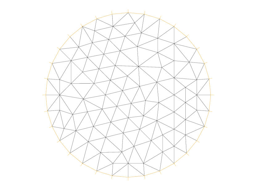
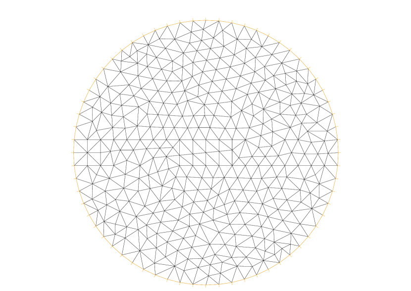
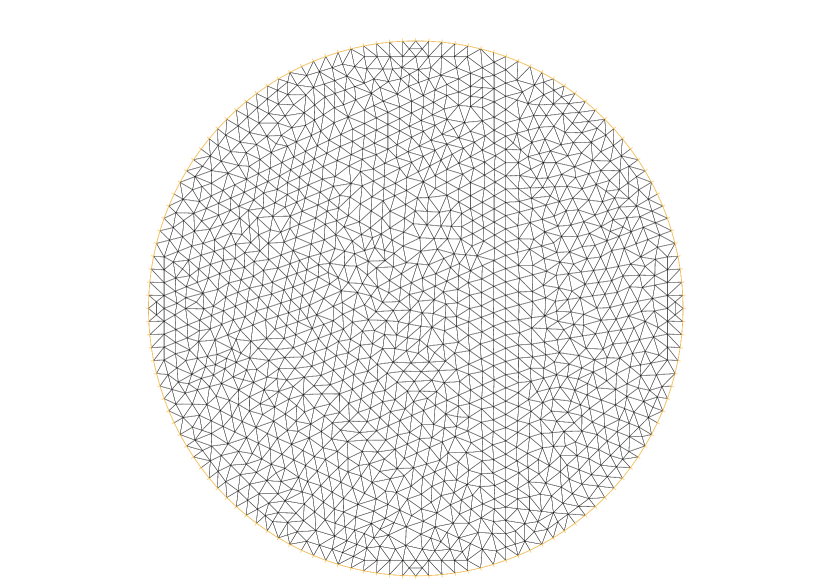
Figure 1: The FEM meshes with $M=16$, $M=32$ and $M=64$, respectively.

Table 3: $L^{2}$-norm errors of the linear Galerkin FEM (Example 5.2).

$\displaystyle\tau=\frac{1}{M^{2}}$	$M$	$\displaystyle\|{\bf U}_{h}^{N}-{\bf u}(\cdot,t_{N})\|_{L^{2}}$	$\displaystyle\|{\bf U}_{h}^{N}-{\bf u}(\cdot,t_{N})\|_{H^{1}}$
	16	2.138E-02	1.596E-01
	32	4.845E-03	7.534E-02
	64	1.314E-03	3.633E-02
convergence rate		2.01	1.06

Table 4: $L^{2}$-norm errors of the linear Galerkin FEM with refined meshes (Example 5.2).

$\tau=0.005$	$M$	$\|{\bf U}_{h}^{N}-{\bf u}(\cdot,t_{N})\|_{L^{2}}$	$\|{\bf U}_{h}^{N}-{\bf u}(\cdot,t_{N})\|_{H^{1}}$
	32	2.112E-02	1.644E-01
	64	5.493E-03	8.883E-02
	128	4.882E-03	5.508E-02
$\tau=0.010$	$M$	$\|{\bf U}_{h}^{N}-{\bf u}(\cdot,t_{N})\|_{L^{2}}$	$\|{\bf U}_{h}^{N}-{\bf u}(\cdot,t_{N})\|_{H^{1}}$
	32	2.078E-02	1.897E-01
	64	9.551E-03	1.158E-01
	128	1.020E-02	8.863E-02
$\tau=0.025$	$M$	$\|{\bf U}_{h}^{N}-{\bf u}(\cdot,t_{N})\|_{L^{2}}$	$\|{\bf U}_{h}^{N}-{\bf u}(\cdot,t_{N})\|_{H^{1}}$
	32	2.741E-02	2.862E-01
	64	2.520E-02	2.228E-01
	128	2.654E-02	2.051E-01

Example 5.3   Finally, we consider the equation

$$\frac{\partial u}{\partial t}-\nabla\cdot(\kappa(u)\nabla u)=\sigma(u)|\nabla u|^{4}+f$$ (5.5)

in $\Omega=(0,1)\times(0,1)\times(0,1)$ with $\kappa(u)=1+\sin^{2}u$ and $\sigma(u)=1/(1+u)$. The function $f$ is chosen corresponding to the exact solution

$$u(x,y,t)=100x(1-x)y(1-y)z(1-z)\,\sin(x+2y-z)te^{-t}.$$ (5.6)

which satisfies the homogeneous Dirichlet boundary condition.

A uniform tetrahedral partition with $M+1$ nodes in each direction is used in our computation (with $h=\sqrt{3}/M$). We solve the system by the proposed method up to the time $t=1$. To illustrate our error estimates, errors of the numerical solution with $\tau=8h^{2}$ are presented in Table 6. Similalry numerical errors with fixed $\tau$ and refined $h$ are presented in Table 6. The same observations can be made here. Again, our numerical results show that the scheme is unconditionally stabe (convergent).

Table 5: $L^{2}$-norm rrors of the linear Galerkin FEM (Example 5.3).

$\tau$	$h$	$\displaystyle\|U_{h}^{N}-u(\cdot,t_{N})\|_{L^{2}}$	$\displaystyle\|U_{h}^{N}-u(\cdot,t_{N})\|_{H^{1}}$
1/8	1/8	2.094E-02	8.379E-02
1/32	1/16	4.996E-03	1.983E-02
1/128	1/32	1.220E-03	4.755E-03
convergence rate		2.08	2.06

Table 6: $L^{2}$-norm errors of the linear Galerkin FEM with refined meshes (Example 5.3).

$\tau=0.025$	$h$	$\|U_{h}^{N}-u(\cdot,t_{N})\|_{L^{2}}$	$\|U_{h}^{N}-u(\cdot,t_{N})\|_{H^{1}}$
	1/8	1.808E-02	6.327E-02
	1/16	4.858E-03	1.879E-02
	1/32	1.549E-03	7.156E-03
$\tau=0.05$	$h$	$\|U_{h}^{N}-u(\cdot,t_{N})\|_{L^{2}}$	$\|U_{h}^{N}-u(\cdot,t_{N})\|_{H^{1}}$
	1/8	1.862E-02	6.707E-02
	1/16	5.478E-03	2.357E-02
	1/32	2.181E-03	1.206E-02
$\tau=0.1$	$h$	$\|U_{h}^{N}-u(\cdot,t_{N})\|_{L^{2}}$	$\|U_{h}^{N}-u(\cdot,t_{N})\|_{H^{1}}$
	1/8	2.008E-02	7.762E-02
	1/16	7.241E-03	3.759E-02
	1/32	3.976E-03	2.668E-02

6 Conclusion

We have presented unconditionally optimal error estimates of a class of linearized Galerkin FEMs for general nonlinear parabolic equations, which may cover many physical applications. The time-step size restriction was always a key issue in previous analysis and practical computation. Our theoretical analysis and numerical results show clearly that no time-step condition is needed for these linearized Galerkin FEMs. Our approach is based on a priori estimates of the numerical solution in the $W^{1,\infty}$ norm. With these estimates, optimal error estimates can be proved unconditionally from classical FEM error analysis. Clearly, our approach is applicable to many other time discretization schemes and more general nonlinear equations (systems).

References

- [1] Y. Achdou and J.L. Guermond, Convergence analysis of a finite element projection /Lagrange-Galerkin method for the incompressible Navier-Stokes equations, SIAM J. Numer. Anal., 37 (2000), 799–826.
- [2] S. Agmon, A. Douglis, and L. Nirenberg, Estimates near the boundary for solutions of elliptic partial differential equations satisfying general boundary conditions, Part I and Part II, Comm. Pure Appl. Math., 12 (1959), 623–727; 127 (1964), 35–92.
- [3] G.D. Akrivis, V.A. Dougalis and O.A. Karakashian, On fully discrete Galerkin methods of second-order temporal accuracy for the nonlinear Schrödinger equation, Numer. Math., 59 (1991), 31–53.
- [4] W. Allegretto, Y. Lin and S. Ma, Existence and long time behaviour of solutions to obstacle thermistor equations, Discrete and Continuous Dynamical Syst., Series A, 8 (2002), 757–780.
- [5] W. Bao and Y. Cai, Uniform error estimates of finite difference methods for the nonlinear Schrödinger equation with wave operator, SIAM J. Numer. Anal., 50 (2012), 492–521.
- [6] S.S. Byun and L. Wang, Elliptic equations with measurable coefficients in Reifenberg domains, Advances in Mathematics, 225 (2010), 2648–2673.
- [7] J.R. Cannon and Y. Lin, Nonclassical projection and Galerkin methods for nonlinear parabolic integro-differential equations, Calcolo, 25 (1988), 187–201.
- [8] Z. Chen and K. -H. Hoffmann, Numerical studies of a non-stationary Ginzburg-Landau model for superconductivity, Adv. Math. Sci. Appl., 5 (1995), 363–389.
- [9] Ya-Zhe Chen and Lan-Cheng Wu, Second Order Elliptic Equations and Elliptic Systems, Translations of Mathematical Monographs 174, AMS 1998, USA.
- [10] Z. Deng and H. Ma, Optimal error estimates of the Fourier spectral method for a class of nonlocal, nonlinear dispersive wave equations, Appl. Numer. Math., 59 (2009), 988–1010.
- [11] J. Douglas, JR., R. Ewing and M.F. Wheeler, A time-discretization procedure for a mixed finite element approximation of miscible displacement in porous media, RAIRO Anal. Numer., 17 (1983), 249–265.
- [12] T. Dupont, G. Fairweather and J.P. Johnson, Three-level Galerkin methods for parabolic equations, SIAM J. Numer. Anal., 11 (1974), 392–410.
- [13] R.G. Durán, On the approximation of miscible displacement in porous media by a method of characteristics combined with a mixed method, SIAM J. Numer. Anal., 25 (1988), 989–1001.
- [14] C.M. Elliott, and S. Larsson, A finite element model for the time-dependent Joule heating problem, Math. Comp., 64 (1995), 1433–1453.
- [15] V.J. Ervin, W.W. Miles, Approximation of time-dependent viscoelastic fluid flow: SUPG approximation, SIAM J. Numer. Anal., 41 (2003), 457–486.
- [16] R.E. Ewing and M.F. Wheeler, Galerkin methods for miscible displacement problems in porous media, SIAM J. Numer. Anal., 17 (1980), 351–365.
- [17] X. Feng, Y. He and C. Liu, Analysis of finite element approximation of a phasse field model for two-phase fluids, Math. Comput., 258 (2007), 539–571.
- [18] Yinnian He, The Euler implicit/explicit scheme for the 2D time-dependent Navier-Stokes equations with smooth or non-smooth initial data, Math. Comp., 77 (2008), 2097–2124. Convergence Joule heating 50 (2010),
- [19] Y. Hou, B. Li and W. Sun, Error analysis of splitting Galerkin methods for heat and sweat transport in textile materials, SIAM J. Numer. Anal., to appear.
- [20] B. Kellogg and B. Liu, The analysis of a finite element method for the Navier–Stokes equations with compressibility, Numer. Math., 87 (2000), 153–170.
- [21] O.A. Ladyzenskaja, V.A. Solonnikov, and N.N. Uralceva, Linear and quasilinear equations of parabolic type, Translations of Mathematical Monographs 23, Providence, 1968.
- [22] B. Li and W. Sun, Error analysis of linearized semi-implicit Galerkin finite element methods for nonlinear parabolic equations, Int. J. Numer. Anal. Modeling, 10 (2013), 622–633.
- [23] B. Li and W. Sun, Unconditional convergence and optimal error estimates of a Galerkin-mixed FEM for incompressible miscible flow in porous media, submitted (http://arxiv.org/abs/1207.1762v2).
- [24] B. Li, Mathematical modelling, analysis and computation for some complex and nonlinear flow problems, PhD Thesis, City University of Hong Kong, Hong Kong, July, 2012.
- [25] B. Liu, The analysis of a finite element method with streamline diffusion for the compressible Navier–Stokes equations, SIAM J. Numer. Anal., 38 (2000), 1–16.
- [26] H. Ma and W. Sun, Optimal error estimates of the Legendre-Petrov-Galerkin method for the Korteweg-de Vries equation, SIAM J. Numer. Anal., 39 (2001), 1380–1394.
- [27] M. Mu and Y. Huang, An alternating Crank-Nicolson method for decoupling the Ginzburg-Landau equations, SIAM J. Numer. Anal., 35 (1998), 1740–1761.
- [28] R. Rannacher and R. Scott, Some optimal error estimates for piecewise linear finite element approximations, Math. Comp., 38 (1982), 437–445.
- [29] J. Shen, On an unconditionally stable scheme for the unsteady Navier–Stokes equations, J. Comput. Math., 8(1990), 276–288.
- [30] C.G. Simader, On Dirichlet Boundary Value Problem. An Theory Based on a Generalization of Garding’s Inequality, Lecture Notes in Math., vol. 268, Springer, Berlin, 1972.
- [31] W. Sun and Z. Sun, Finite difference methods for a nonlinear and strongly coupled heat and moisture transport system in textile materials, Numer Math., 120 (2012), 153–187.
- [32] V. Thomée, Galerkin finite element methods for parabolic problems, Springer-Verkag Berkub Geudekberg 1997.
- [33] Y. Tourigny, Optimal estimates for two time-discrete Galerkin approximations of a nonlinear Schrödinger equation, IMA J. Numer. Anal., 11 (1991), 509-523.
- [34] H. Wang, An optimal-order error estimate for a family of ELLAM-MFEM approximations to porous medium flow, SIAM J. Numer. Anal., 46 (2008), 2133–2152.
- [35] K. Wang, Y. He and Y. Shang, Fully discrete finite element method for the viscoelastic fluid motion equations, Discrete Contin. Dyn. Syst. Ser. B, 13 (2010), 665–684.
- [36] M.F. Wheeler, A priori error estimates for Galerkin approximations to parabolic partial differential equations, SIAM J. Numer. Anal., 10 (1973), 723–759.
- [37] H. Wu, H. Ma and H. Li, Optimal error estimates of the Chebyshev-Legendre spectral method for solving the generalized Burgers equation, SIAM J. Numer. Anal., 41 (2003), 659–672.
- [38] X.Y. Yue, Numerical analysis of nonstationary thermistor problem, J. Comput. Math., 12 (1994), 213–223.
- [39] Z.Q. Zhang and H. Ma, A rational spectral method for the KdV equation on the half line, J. Comput. Appl. Math., 230 (2009), 614–625.
- [40] W. Zhao, Convergence analysis of finite element method for the nonstationary thermistor problem, Shandong Daxue Xuebao, 29 (1994), 361–367.
- [41] M. Zlámal, Curved elements in the finite element method. I∗, SIAM J. Numer. Anal., 10 (1973), 229–240.
- [42] G.E. Zouraris, On the convergence of a linear two-step finite element method for the nonlinear Schrödinger equation, M2AN Math. Model. Numer. Anal., 35 (2001), 389–405.