A new variable in scalar cosmology with exponential potential

Abstract

We present a new way describing the solution of the Einstein-scalar field theory with exponential potential $V\propto e^{\sqrt{6}\beta\phi/M_{Pl}}$ in spatially flat Friedmann-Robertson-Walker space-time. We introduced a new time variable, $L$, which may vary in $[-1,1]$. The new time represents the state of the universe clearly because the equation of state at a given time takes the simple form, $w=-1+2L^{2}$. The universe will inflate when $|L|<1/\sqrt{3}$. For $\beta\leq 1$, the universe ends with its evolution at $L=\beta$. This implies that the equation of state at the end of the universe is nothing but $w=-1+2\beta^{2}$. For $\beta\geq 1$, the universe ends at $L=1$, where the equation of state of the universe is one. On the other hand, the universe always begins with $w=1$ at $L=\pm 1$.

The discovery of cosmic acceleration in 1997, which is regarded to be originated from a dark energy, changed the modern cosmology from the basics. In the context of fundamental theories, it is an important problem to understand the origin of the dark energy. The dimensional reduction of higher dimensional M/string theory typically give rise to a scalar fields with exponential potentials coupled to four-dimensional gravity. It is usually argued that these the homogeneous scalar field slowly rolling on the potential may give rise to a dark energy, which is typically called as quintessence Caldwell:1998je ; quint . It is interesting to understand whether exponential potentials could describe observational data for the late-time cosmic acceleration.

In cosmology, exponential potentials were much investigated in the past and general exact solutions have appeared Kehagias:2004bd ; Townsend:2003qv . In particular, a general solution in four dimensions was obtained in Ref. Chimento:1998ju . Especially, in Ref. Russo:2004ym , it was also shown that in the simplest case of a homogeneous scalar field coupled to an exponential potential can be solved in a direct way in $d$-dimensions by introducing new variables which decouple the system. In Ref. Townsend:2003fx , it was shown an example of cosmology which starts with a decelerating expansion, at some point it experiences a transitory period of acceleration, and it ends with decelerating expansion again. The origin of the acceleration was further clarified in Ref. Emparan:2003gg . As noted in Ref. Russo:2004ym , the explicit general solution will present a clear view in parametric space on the physical origin of the acceleration.

We are interested in the universe which is spatially flat, homogeneous, and isotropic, with metric:

$$ds^{2}=-dt^{2}+a^{2}(t)(dx^{2}+dy^{2}+dz^{2}),$$ (1)

where $a(t)$ is the scale factor. We find exact cosmological solutions of Einstein equation coupled to a scalar field $\phi$ with action in standard form,

$$S=\int d^{4}x\sqrt{-g}\left[\frac{M_{Pl}^{2}}{2}\,R+\frac{1}{2}g^{\mu\nu}\partial_{\mu}\phi\partial_{\nu}\phi+V(\phi)\right],$$ (2)

where we set $M_{Pl}^{2}=1/(8\pi G)$. The dynamics of the scalar field and gravity can be dealt with a pair of equations

$$3M_{Pl}^{2}H^{2}=\frac{\dot{\phi}^{2}}{2}+V(\phi),$$ (3)

$$\ddot{\phi}+3H\dot{\phi}+V^{\prime}(\phi)=0,$$ (4)

where overdot and prime denote derivatives with respect to time and the scalar field, respectively, and $H=\dot{a}/a$ is the Hubble parameter. We consider the exponential potential,

$$V(\phi)=3M_{Pl}^{2}H_{0}^{2}\,e^{\frac{\sqrt{6}\beta}{M_{Pl}}\phi}.$$ (5)

Without loss of generality we set $\beta>0$. In the case of an exponential potentials, the scalar cosmology in four dimensions were investigated exponential and general exact solutions were found sol ; Russo:2004ym . Interesting properties of the cosmological solutions with exponential solutions were also discussed Copeland:1997et ; ex prpty ; odinsov .

In Refs. Kim:2012dn ; Reyes:2008av ; fakesugra ; Aref'eva:2005fu ; vernov2 , it was shown that the equations of motion (3) and (4) is equivalent to the ‘generating equation’:

$$V(\phi)=3G^{2}(\phi)-2M_{Pl}^{2}[G^{\prime}(\phi)]^{2},$$ (6)

which is typically called as the Hamilton-Jacobi equation, supplemented by

$$\dot{\phi}=-2M_{Pl}G^{\prime}(\phi),\qquad H=\frac{\dot{a}}{a}=\frac{G(\phi)}{M_{Pl}}.$$ (7)

Summarizing, the two coupled differential equations (3) and (4) with respect to time is reduced to one non-linear first order differential equation (6) with respect to the scalar field supplemented by the equation giving the dynamics (7). We solve Eq. (6) directly to obtain the generating function in the cases of the exponential potentials.

One may easily guess a specific solution of the generating function since the derivative of the exponential is nothing but an exponential:

$$G(\phi)=\frac{M_{Pl}H_{0}}{\sqrt{1-\beta^{2}}}e^{\sqrt{\frac{3}{2}}\frac{\beta\phi}{M_{Pl}}},$$ (8)

where a real generating function of this form exists only when $|\beta|<1$. This example was dealt in Ref. Reyes:2008av and its fixed point properties including contributions from perfect fluid were studied in Ref. Copeland:1997et . The scalar field and scale factor corresponding to this is given by

$$\phi(t) = -\sqrt{\frac{2}{3}}\frac{M_{Pl}}{\beta}\log\left(1+\frac{3\beta^{2}H_{0}}{\sqrt{1-\beta^{2}}}t\right),$$

$$a(t) = a_{0}\left(1+\frac{3\beta^{2}H_{0}}{\sqrt{1-\beta^{2}}}t\right)^{\frac{1}{3\beta^{2}}}.$$ (9)

The whole cosmological solutions with the potential (5) were studied in Ref. Russo:2004ym by changing the equations into two Riccati equations using a couple of coordinates transformation. The model was also studied in terms of Nöether charge method in Ref. Ritis and Hamilton-Jacobi method Salopek:1990jq . The model is extended to include a perfect fluid numerically in Ref. Copeland:1997et ; Kehagias:2004bd . The solution (A new variable in scalar cosmology with exponential potential) corresponds to a solution approaching to the fixed point $(x,y)=(\lambda/\sqrt{6},(1-\lambda^{2}/6)^{1/2})$ in Ref. Copeland:1997et . Another two fixed points $(\pm 1,0)$ in the reference corresponds to $V=0$, which is not relevant at the present situation.

In this work, we present the whole generating functions by solving Eq. (6) directly. The general solution of Eq. (6) representing expanding universe is

$$M_{Pl}H=G(L)=M_{Pl}H_{0}e^{\sqrt{\frac{3}{2}}\frac{\beta\phi_{c}}{M_{Pl}}}\frac{|1-L/\beta|^{\frac{\beta^{2}}{1-\beta^{2}}}}{(1-L)^{\frac{1}{2(1-\beta)}}(1+L)^{\frac{1}{2(1+\beta)}}},$$ (10)

where we restrict the range of $L$ to be $|L|\leq 1$. For the range of $|L|>1$, the generating function describes the potential $V(\phi)=-3M_{Pl}^{2}H_{0}^{2}e^{\sqrt{6}\frac{\beta\phi}{M_{Pl}}}$, which we are not interested in at the present cosmological situation. $\phi_{c}$ is chosen to be a parameter characterizing the maximum possible value of the scalar field during evolution, which will be shown below, and the scalar field evolves as

$$\frac{\phi}{M_{Pl}}=\frac{\phi_{c}}{M_{Pl}}+\frac{1}{\sqrt{6}}\left[\frac{2\beta}{1-\beta^{2}}\log|1-L/\beta|-\frac{1}{1-\beta}\log(1-L)+\frac{1}{1+\beta}\log(1+L)\right].$$ (11)

For $\beta=1$, this equation is ill-defined. But, by using $\beta\to 1$ limit, we get

$$\frac{\phi}{M_{Pl}}=\frac{\phi_{c}}{M_{Pl}}-\frac{L}{\sqrt{6}(1-L)}+\frac{1}{2\sqrt{6}}\log\frac{1+L}{1-L}.$$ (12)

The solution (A new variable in scalar cosmology with exponential potential) corresponds to the limit $\phi_{c}\to\infty$ with $L=\beta$. The schematic plot for the time evolution of the scalar field is given in Fig. 1.

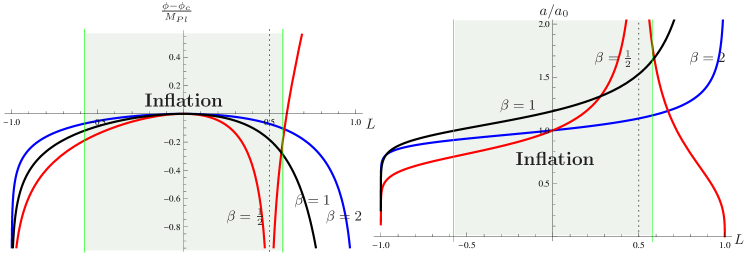
Figure 1: Schematic plot of the evolution of the scalar field and the scale factor with respect to $L$. The red, black, and blue curves for $\beta=1/2$, $1$, and $2$, respectively, denote the typical behaviors of the scalar field and the scale factor for the cases with $0<\beta<1$, $\beta=1$, and $\beta>1$. Inside the shaded region, the universe inflates.

The equation of state parameter of the universe can be expressed in a quite simple form:

$$w\equiv\frac{p}{\rho}=-1+\frac{4}{3}\frac{M_{Pl}^{2}G^{\prime}(\phi)^{2}}{G^{2}(\phi)}=-1+\frac{4}{3}\left(\frac{M_{Pl}\frac{dL}{d\phi}\frac{dG(L)}{dL}}{G(L)^{2}}\right)^{2}=-1+2L^{2}.$$ (13)

Because of the simplicity, it becomes easier to understand the behavior of the universe as a function of $L$. The equation of state becomes that of the cosmological constant at $L=0$. The universe inflates if $w<-1/3$, which gives $-1/\sqrt{3}<L<1/\sqrt{3}$.

The relation between the cosmological time and the time $L$ is explicitly given in Appendix A. Rather than explicitly describing the whole detail, let us remind the following key results: For $\beta<1$, there are two corresponding universes. One begins at $L=-1$ ($t=0$) and ends at $L=\beta$ ($t=\infty$) and the other begins at $L=+1$ ($t=0$) and ends at $L=\beta$ ($t\to\infty$). Remember that the time arrow is reversed in the second case. For $\beta\geq 1$, the universe begins at $L=-1$ ($t=0$) and ends at $L=1$ ($t=\infty$). Noting $H=a^{-1}da/dt$, the scale factor, using Eq. (20) in Appendix A, is given by

$$\frac{1}{a}\frac{da}{dL}=\frac{dt}{dL}H=\frac{1}{3}\frac{1}{(1-L^{2})(\beta-L)}.$$ (14)

Integrating, we get the scale factor as a function of $L$,

$$a(L)=a_{0}\frac{(1-L)^{\frac{1}{6(1-\beta)}}(1+L)^{\frac{1}{6(1+\beta)}}}{|1-L/\beta|^{\frac{1}{3(1-\beta^{2})}}}.$$ (15)

The metric (1), now, can be written as,

$$ds^{2}=-\frac{1}{9\beta^{2}H_{0}^{2}e^{\sqrt{6}\frac{\beta\phi_{c}}{M_{Pl}}}}\frac{(1-L)^{\frac{2\beta-1}{1-\beta}}}{(1+L)^{\frac{2\beta+1}{1+\beta}}|1-L/\beta|^{\frac{2}{1-\beta^{2}}}}dL^{2}+a_{0}^{2}\frac{(1-L)^{\frac{1}{3(1-\beta)}}(1+L)^{\frac{1}{3(1+\beta)}}}{|1-L/\beta|^{\frac{2}{3(1-\beta^{2})}}}(dx^{2}+dy^{2}+dz^{2}),$$ (16)

These solutions are not new but found in Ref. Russo:2004ym in a different form. For various specific parameter values, the solutions were also found in Ref. Chimento:1998ju . In the rest of this work, we analyze the behavior of the universe for each parameter space.

.0.1 $0<\beta<1$ case

Let us consider the case with $0<\beta<1$ first. Because the scale factor at $L=\beta$ diverges, there are two independent universes divided by the range of $L$ with $-1\leq L<\beta$ and $\beta<L\leq 1$, in which the time runs in $(0,\infty)$.

First consider the universe resides in $-1\leq L<\beta$. The universe begins at $L=-1$ with $\phi\to-\infty$. The universe is in a singular state because the scalar energy density diverges, which can be seen from Eq. (19). As the scalar field climbs up the potential, its velocity monotonically decreases due to the friction of the Hubble parameter and the inclination of the potential. The Hubble parameter also decreases until $L$ reaches $L=1/\sqrt{3}$. At this time, the universe starts to inflate because the speed of the scalar field is slowed down and the scalar potential is big enough. The scalar field arrive at $\phi=\phi_{c}$ at time $L=0$ and its velocity vanishes there. Thereafter, it turns its direction and starts to decrease. However, note that the scalar velocity vanishes at $L=\beta$. Therefore, even if the scalar field decreases continually, its velocity approaches zero in the future. This results in a interesting result: If $\beta\leq 1/\sqrt{3}$, the universe inflates eternally even though the scalar field continually decreases so that the scalar potential goes to zero. On the other hand, if $\beta>1/\sqrt{3}$, the inflation will end at $L=1/\sqrt{3}$ and the universe enters into the decelerating expansion. The universe will ends at $L=\beta$. Therefore, the equation of state at the end of the universe is simply given by

$$w=-1+2\beta^{2}.$$

Let us obtain the asymptotic form of the scalar field and the scale factor for $L\sim\beta$. The asymptotic form, in fact, is given by the fixed point solution (A new variable in scalar cosmology with exponential potential). Then, from Eq. (11), one gets

$$\frac{(\phi-\phi_{c})}{M_{Pl}}=\frac{1}{\sqrt{6}}\left(\frac{\log(1+\beta)}{1+\beta}-\frac{\log(1-\beta)}{1-\beta}\right)+\sqrt{\frac{2}{3}}\frac{\log(1-L/\beta)}{1-\beta^{2}}.$$

Then, one can integrate Eqs. (10) and (19) to obtain the same evolutions of the scale factor and the scalar field as in Eq. (A new variable in scalar cosmology with exponential potential). For $\beta<1/\sqrt{3}$, the attractor denotes the inflationary attractor. On the other hand, for $\beta\geq 1/\sqrt{3}$, it is not an inflationary attractor but is still an attractor approaching a state with its equation of state $w=-1+2\beta^{2}$.

We next consider the case with $\beta\leq L\leq 1$. The universe begins at $L=1$ with $\phi\to\infty$ and $a=0$. At the beginning, the universe starts from a singular state. Even though the scalar field slides down the potential, its speed cannot always increase because the friction due to the Hubble parameter competes with the slope of the potential. The scalar velocity starts to decrease at some $\phi$. At $L=1/\sqrt{3}$, its speed becomes small enough to support the inflation of the universe. If $\beta<1/\sqrt{3}$, the universe will go into eternal inflating stage at $L=1/\sqrt{3}$. On the other hand, if $\beta>1/\sqrt{3}$, the universe fails to get into the inflating stage but continues the decelerating expansion. The later evolutions can also be approximated by the fixed point solution (A new variable in scalar cosmology with exponential potential).

.0.2 $\beta>1$ case

The cosmological time runs $(0,\infty)$ during $-1\leq L\leq 1$. The universe begins at $L=-1$ with $\phi\to-\infty$ and $a=0$. At the beginning, the universe starts from a singular state. As the scalar field climbs up the potential, the velocity (therefore kinetic energy) of the scalar field decreases due to the friction of the Hubble parameter and the slope of the potential. For $-1/\sqrt{3}<L<1/\sqrt{3}$, the kinetic energy is small enough to inflate the universe. The velocity vanishes at $\phi=\phi_{c}$, when $L=0$. Afterward, the scalar field starts to slide down the potential. However, as seen in Eq. (19), the scalar velocity vanishes at $L=1$. Therefore, it cannot increase at all times but starts to decrease at some field value. In the future, the scalar velocity goes to zero as $\phi\to-\infty$. The universe, after the temporal inflation, goes into decelerating expansion.

Let us now consider the asymptotic behavior of the solutions in the cosmological time. We first consider the early universe around $L\sim-1$. Using Eq. (22), the scalar field and the scale factor behaves as

$$\phi(t) \to \phi_{i}+\sqrt{\frac{2}{3}}M_{Pl}\,\log\big{(}H_{0}t\big{)},\qquad a(t)\to a_{i}\,\Big{(}3H_{0}t\Big{)}^{1/3}.$$ (17)

where $\phi_{i}=(\beta+1)\phi_{c}+\sqrt{\frac{2}{3}}M_{Pl}\log\left(\frac{3}{\sqrt{2}}\frac{2^{\frac{\beta+1}{2(\beta-1)}}}{(1+\beta^{-1})^{\frac{\beta}{\beta-1}}}\right)$ is a lengthy function of $\phi_{c}$ and $\beta$ and

$$a_{i}=a_{0}e^{\frac{\beta\phi_{c}}{\sqrt{6}M_{Pl}}}\left(1+\frac{1}{\beta}\right)^{-1/3}.$$

We next consider the later time solution with $L\sim 1$. As $t\to\infty$, the scalar field and the scale factor behaves as

$$\phi(t) \to \phi_{f}-\sqrt{\frac{2}{3}}M_{Pl}\log\Big{(}H_{0}t\Big{)},\qquad a(t)\to a_{f}\,\Big{(}3H_{0}t\Big{)}^{1/3}.$$ (18)

where $\phi_{f}=(\beta-1)\phi_{c}-\sqrt{\frac{2}{3}}M_{Pl}\log\left(\frac{3}{\sqrt{2}}\frac{2^{\frac{\beta-1}{2(\beta+1)}}}{(1-\beta^{-1})^{\frac{\beta}{\beta+1}}}\right)$ is a lengthy function of $\phi_{c}$ and $\beta$ and

$$a_{f}=a_{0}e^{\frac{\beta\phi_{c}}{\sqrt{6}M_{Pl}}}\left(1-\frac{1}{\beta}\right)^{-1/3}.$$

Comparing $a_{i}$ and $a_{f}$, we find that the scale factor during the inflationary period is enhanced by

$$\frac{a_{f}}{a_{i}}=\Big{(}\frac{\beta+1}{\beta-1}\Big{)}^{1/3}.$$

Unless $\beta-1\sim 10^{-90}$, this value is not big enough to support the present observational data for inflation.

The asymptotic form of the scalar field and the scale factor are explicitly dependent on the choice of $\phi_{c}$ and deviates from the fixed point solution (A new variable in scalar cosmology with exponential potential). In fact, this corresponds to a kinetic attractor, with the equation of state $p=\rho$ corresponding to matter with dominance of kinetic energy with equation of state, $w\longrightarrow 1.$

.0.3 $\beta=1$ case

The solution in this case can be obtained by taking the $\beta\to 1$ limit in Eq. (15). The evolution of the scalar field was given in Eq. (12). The derivative of the scale factor with respect to $L$ is the same as in Eq. (14) with $\beta=1$. Integrating this equation with Eq. (A), we get the scale factor,

$$a(L)=a_{0}\left(\frac{1+L}{1-L}\right)^{1/12}\exp\left[\frac{1}{6(1-L)}\right].$$

The equation of state is also the same as Eq. (13).

As $-1\leq L\leq 1$, the cosmological time runs $(0,\infty)$. The universe begins from $L=-1$ with $a=0$ and $\phi=-\infty$. Both of the initial scalar velocity and Hubble parameter diverges. Due to the friction from the Hubble parameter, the scalar velocity decreases with time and the scalar field starts to approach $\phi_{c}$. At $-1/\sqrt{3}<L<1/\sqrt{3}$, the scalar velocity becomes small enough to support the inflation. The scalar field takes its maximum value $\phi_{c}$ at $L=0$ and then bounces back to decrease.

On the whole, the evolution of the scale factor and the scalar field is completely different from that of $\beta\neq 1$.

We now write down the asymptotic form of the solutions for $L\sim-1$ using Eq. (25),

$$\phi=\phi_{c}+\frac{1}{2\sqrt{6}}\Big{(}1-\log 2+4\log(2H_{1}t)\Big{)}-\frac{8}{\sqrt{6}\,e\,(2H_{1}t)^{4}}\qquad a(t)=a_{0}\left(\frac{e}{4}\right)^{1/6}(2H_{1}t)^{1/3}.$$

On the other hand, around $L\sim 1$ using Eq. (26), the scale factor becomes

$$a(t)=2^{1/12}a_{0}\left[2H_{1}t\log\big{(}H_{1}t\big{)}\right]^{1/3}+\cdots$$

where $H_{1}=3/2\times H_{0}\,e^{\sqrt{\frac{3}{2}}\phi_{c}/M_{Pl}}$. Notice that the limiting behaviors are completely different from the cases of $\beta\neq 1$. This limiting behavior can also be seen in the specific solutions in Ref. Chimento:1998ju .

In summary, we directly attacked the Hamilton-Jacobi equation for the scalar cosmology with exponential potential $V\propto e^{\sqrt{6}\beta\phi/M_{Pl}}$. We have reproduced the known solutions and introduced a new time variable $L$, which varies in $-1\leq L\leq 1$. In describing the evolution of the universe, we have found that the new time variable is very convenient to identify the state of the universe at a given time. The most beautiful property of it is that the equation of state of the scalar field is determined by the value very easily, $w=-1+2L^{2}$. From this, we notice that the universe will expands with accelerating rate if $-1/\sqrt{3}<L<1/\sqrt{3}$.

The evolution of the universe are characterized by the value of $\beta$. For $0<\beta<1$, the universe ends at $L=\beta$. Therefore, the equation of state at the end of the universe is nothing but $w=-1+2\beta^{2}$. For $0<\beta\leq 1/\sqrt{3}$ the universe ends with eternal later time inflation irrespective of the initial condition of the scalar field. On the other hand, for $\beta>1$, the universe will ends at $L=1$ and the equation of state of the universe will approach to $w=1$, implying the kinetic dominance. The temporal inflation during $-1/\sqrt{3}<L<1/\sqrt{3}$ makes the scale factor is increased by the factor $\big{[}(\beta+1)/(\beta-1)\big{]}^{1/3}$. However, this is not enough to explain the cosmic inflation or the present later time accelerating expansion. To see how useful the variable $L$ in describing the scalar cosmology is, more general systems need to be analyzed. For example, in addition to the scalar field one may include a perfect fluid, an axion Sonner:2006yn , or a gauge field Maeda:2012eg .

If the scalar field plays the role of the dark energy, the value of $\beta$ should be very close to zero, $\beta\ll 1$ for dark energy dominated future. However, as pointed out by Townsend Townsend:2003qv , there is a conjecture saying that such spacetime with future event horizon cannot arise from classical compactification of String/M-theory. For partial proof for this conjecture, consult Ref. Teo:2004hq . If this is true, the value should be restricted to be $\beta\geq 1/\sqrt{3}$ discarding the previous possibility.

Appendix A The cosmological time and $L$

From Eq. (7), the time derivative of the scalar field is given by

$$\dot{\phi}=-2M_{Pl}\frac{dG}{d\phi}=-2M_{Pl}\frac{dL}{d\phi}\frac{dG(L)}{dL}=-\sqrt{6}M_{Pl}H_{0}\,e^{\sqrt{\frac{3}{2}}\frac{\beta\phi_{c}}{M_{Pl}}}\frac{L|1-L/\beta|^{\frac{\beta^{2}}{1-\beta^{2}}}}{(1-L)^{\frac{1}{2(1-\beta)}}(1+L)^{\frac{1}{2(1+\beta)}}}.$$ (19)

where we have used Eq. (11) to get

$$\frac{d\phi}{dL}=-M_{Pl}\sqrt{\frac{2}{3}}\frac{L}{(\beta-L)(1-L^{2})}.$$

Now, we obtain the relation between the two times $L$ and $t$ by

$$3\beta H_{0}\,e^{\sqrt{\frac{3}{2}}\frac{\beta\phi_{c}}{M_{Pl}}}\,dt=\frac{(1-L)^{\frac{2\beta-1}{2(1-\beta)}}}{(1-L/\beta)|1-L/\beta|^{\frac{\beta^{2}}{1-\beta^{2}}}(1+L)^{\frac{2\beta+1}{2(1+\beta)}}}dL.$$ (20)

Note that the arrow of time of the two time is dependent on the sign of $\beta-L$. Because the exponent of $1/(\beta-L)$ is always larger than $1$, we see that the cosmological time go to infinity at $L=\beta$. At $L=-1$, the exponent of $1/(L+1)$ is always smaller than one for positive $\beta$. Therefore, the time will take a finite value, which we choose to zero. At $L=1$, the exponent of $1/(1-L)$ is equal to or larger than one if $\beta\geq 1$. Therefore, $t\to\infty$ for $\beta\geq 1$ and $t$ takes a finite value for $\beta<1$, which we choose to zero. Explicitly, Eq. (20) can be integrated in a closed form,

$$t = t_{0}+\frac{1}{3\beta H_{0}}\frac{\mbox{sign}(\beta-L)\,2^{-\frac{2\beta-1}{2\beta+2}}}{e^{\sqrt{\frac{3}{2}}\frac{\beta\phi_{c}}{M_{Pl}}}(\beta-1)^{\frac{\beta^{2}}{1-\beta^{2}}}}(1-L)^{\frac{1}{2-2\beta}}$$ (21)

$$\times\Big{[}\frac{L-1}{2\beta-3}F_{1}\left(\frac{3-2\beta}{2-2\beta};\frac{2\beta+1}{2\beta+2},\frac{1}{1-\beta^{2}};\frac{5-4\beta}{2-2\beta};\frac{1-L}{2},\frac{L-1}{\beta-1}\right)$$

$$~{}~{}+2F_{1}\left(\frac{1}{2-2\beta};-\frac{1}{2\beta+2},\frac{1}{1-\beta^{2}};\frac{3-2\beta}{2-2\beta};\frac{1-L}{2},\frac{L-1}{\beta-1}\right)\Big{]},$$

where $t_{0}$ will be used to set the initial time to be zero. However, it is too complex to use directly. We may simply note that the arrow of the time is the same as the increase of $L$ for $L<\beta$ and is reversed for $L>\beta$ and use the asymptotic forms below. Around $L\to-1$, the relation becomes,

$$L\to-1+\frac{e^{\sqrt{6}\beta(\beta+1)\phi_{c}/M_{Pl}}}{2^{\frac{\beta+1}{\beta-1}}(1+\beta^{-1})^{\frac{2\beta^{2}}{\beta-1}}}\Big{(}3H_{0}t\Big{)}^{2(1+\beta)}.$$ (22)

Around $L\to 1$, Eq. (21) becomes

$$L\to 1-\frac{e^{\sqrt{6}\beta(1-\beta)\phi_{c}/M_{Pl}}}{2^{\frac{\beta-1}{\beta+1}}(1-\beta^{-1})^{\frac{2\beta^{2}}{\beta+1}}}\Big{(}3H_{0}t\Big{)}^{2(1-\beta)}.$$ (23)

Now we write down the evolutions in $\beta=1$ case. With $\beta\to 1$ limit, the generating function becomes

$$G(L)=M_{Pl}H_{0}e^{\sqrt{\frac{3}{2}}\frac{\beta\phi_{c}}{M_{Pl}}}\frac{e^{-\frac{L}{2(1-L)}}}{(1+L)^{1/4}(1-L)^{3/4}}.$$

The time derivative of the scalar field and $L$ with respect to the cosmological time is given by

$$\dot{\phi}=-\sqrt{6}M_{Pl}H_{0}e^{\sqrt{\frac{3}{2}}\frac{\phi_{c}}{M_{Pl}}}\frac{L\,e^{-\frac{L}{2(1-L)}}}{(1-L)^{3/4}(1+L)^{1/4}},$$

$$3H_{0}e^{\sqrt{\frac{3}{2}}\frac{\phi_{c}}{M_{Pl}}}\,dt=\frac{e^{\frac{L}{2(1-L)}}}{(1+L)^{3/4}(1-L)^{5/4}}\,dL.$$ (24)

For $L\to-1$, the second equation of Eq. (A) becomes

$$L+1=\frac{e}{2^{3}}(2H_{1}t)^{4}.$$ (25)

For $L\to 1$, the relation with the cosmological time becomes

$$3H_{0}e^{\sqrt{\frac{3}{2}}\frac{\phi_{c}}{M_{Pl}}}t=2(1-L)^{3/4}e^{\frac{1}{2(1-L)}}.$$ (26)

References

- (1) R. R. Caldwell, R. Dave and P. J. Steinhardt, Astrophys. Space Sci. 261, 303 (1998).
- (2) R. R. Caldwell, R. Dave and P. J. Steinhardt, Phys. Rev. Lett. 80, 1582 (1998) [astro-ph/9708069]; N. A. Bahcall, J. P. Ostriker, S. Perlmutter and P. J. Steinhardt, Science 284, 1481 (1999) [astro-ph/9906463]; E. J. Copeland, M. Sami and S. Tsujikawa, Int. J. Mod. Phys. D 15, 1753 (2006) [hep-th/0603057].
- (3) P. K. Townsend, “Cosmic acceleration and M theory,” in :Proceedings of ICMP2003, Lisbon, hep-th/0308149.
- (4) A. Kehagias and G. Kofinas, Class. Quant. Grav. 21, 3871 (2004) [gr-qc/0402059].
- (5) L. P. Chimento, Class. Quant. Grav. 15, 965 (1998).
- (6) J. G. Russo, Phys. Lett. B 600, 185 (2004) [hep-th/0403010].
- (7) P. K. Townsend and M. N. R. Wohlfarth, Phys. Rev. Lett. 91, 061302 (2003) [hep-th/0303097].
- (8) R. Emparan and J. Garriga, JHEP 0305, 028 (2003) [hep-th/0304124].
- (9) Q. Shafi and C. Wetterich, Phys. Lett. B 129, 387 (1983); F. Lucchin and S. Matarrese, Phys. Rev. D 32, 1316 (1985); J. D. Barrow, A. B. Burd, D. Lancaster, Class. Quantum Grav. 3, 551 (1986); A. B. Burd and J. D. Barrow, Nucl. Phys. B 308, 929 (1988); J. J. Halliwell, Phys. Lett. B 185, 341 (1987).
- (10) B. Ratra and P. J. E. Peebles, Phys. Rev. D 37, 3406 (1988); L. P. Chimento, Class. Quant. Grav. 15, 965 (1998). L. P. Chimento, A. E. Cossarini and N. A. Zuccala, Class. Quant. Grav. 15, 57 (1998).
- (11) E. J. Copeland, A. R Liddle and D. Wands, Phys. Rev. D 57, 4686 (1998) [gr-qc/9711068].
- (12) P. K. Townsend and M. N. R. Wohlfarth, Phys. Rev. Lett. 91, 061302 (2003) [hep-th/0303097]; R. Emparan and J. Garriga, JHEP 0305, 028 (2003) [hep-th/0304124].
- (13) E. Elizalde, S. Nojiri, and S. D. Odintsov, Phys. Rev. D 70, 043539 (2004). [arXiv:hep-th/0405034] ; E. Elizalde, S. Nojiri, S. D. Odintsov, D. Saez-Gomez, and V. Faraoni, Phys. Rev. D 77, 106005 (2008). [arXiv:0803.1311 [hep-th]]
- (14) M. A. Reyes, “On exact solutions to the scalar field equations in standard cosmology,” arXiv:0806.2292 [gr-qc].
- (15) D. Bazeia, C. B. Gomes, L. Losano and R. Menezes, Phys. Lett. B 633, 415 (2006) [astro-ph/0512197].
- (16) I. Y. .Aref’eva, A. S. Koshelev and S. Y. .Vernov, Phys. Rev. D 72, 064017 (2005) [astro-ph/0507067].
- (17) S. Y. .Vernov, Teor. Mat. Fiz. 155, 47 (2008) [Theor. Math. Phys. 155, 544 (2008)] [astro-ph/0612487]; I. Y. .Aref’eva, N. V. Bulatov and S. Y. .Vernov, Theor. Math. Phys. 163, 788 (2010) [arXiv:0911.5105 [hep-th]].
- (18) H. -C. Kim, arXiv:1211.0604 [gr-qc].
- (19) R. de Ritis, G. Marmo, G. Platania, C. Rubano, P. Scudellaro and C. Stornaiolo, Phys. Rev. D 42, 1091 (1990).
- (20) D. S. Salopek and J. R. Bond, Phys. Rev. D 42 (1990) 3936.
- (21) J. Sonner, P. K. Townsend and , Phys. Rev. D 74, 103508 (2006) [hep-th/0608068].
- (22) K. -i. Maeda, K. Yamamoto and , Phys. Rev. D 87, 023528 (2013) [arXiv:1210.4054 [astro-ph.CO]].
- (23) E. Teo, Phys. Lett. B 609, 181 (2005) [hep-th/0412164].