Convex Tensor Decomposition via Structured Schatten Norm Regularization

Abstract

We discuss structured Schatten norms for tensor decomposition that includes two recently proposed norms (“overlapped” and “latent”) for convex-optimization-based tensor decomposition, and connect tensor decomposition with wider literature on structured sparsity. Based on the properties of the structured Schatten norms, we mathematically analyze the performance of “latent” approach for tensor decomposition, which was empirically found to perform better than the “overlapped” approach in some settings. We show theoretically that this is indeed the case. In particular, when the unknown true tensor is low-rank in a specific mode, this approach performs as good as knowing the mode with the smallest rank. Along the way, we show a novel duality result for structures Schatten norms, establish the consistency, and discuss the identifiability of this approach. We confirm through numerical simulations that our theoretical prediction can precisely predict the scaling behaviour of the mean squared error.

1 Introduction

Decomposition of tensors (Kolda & Bader, 2009) (or multi-way arrays) into low-rank components arises naturally in many real world data analysis problems. For example, in neuroimaging, we are often interested in finding spatio-temporal patterns of neural activities that are related to certain experimental conditions or subjects; one way to do this is to compute the decomposition of the data tensor, which can be of size channels $\times$ time-points $\times$ subjects $\times$ conditions (Mørup, 2011). In computer vision, an ensemble of face images can be collected into a tensor of size pixels $\times$ subjects $\times$ illumination $\times$ viewpoints; the decomposition of this tensor yields the so called tensorfaces (Vasilescu & Terzopoulos, 2002), which can be regarded as a multi-linear generalization of eigenfaces (Sirovich & Kirby, 1987).

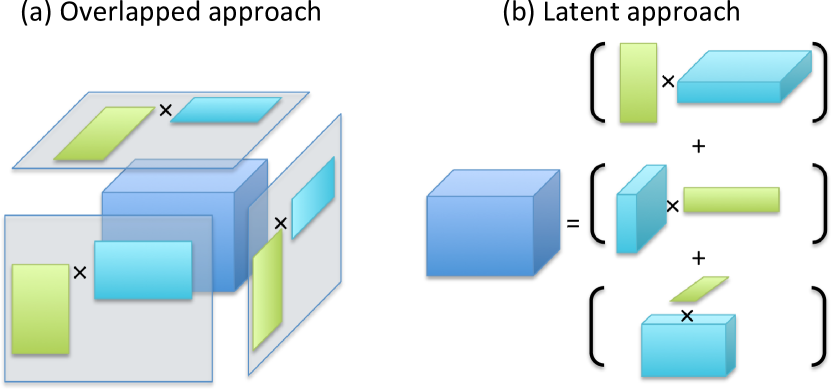
Figure 1: Schematic illustrations of the overlapped approach and the latent approach for the decomposition of a three way tensor ($K=3$).

Conventionally tensor decomposition has been tackled through non-convex optimization problems, using alternate least squares or higher order orthogonal iteration (De Lathauwer et al., 2000). Although being successful in many application areas, the statistical performance of such approaches has been widely open. Moreover, the model selection problem can be highly challenging, especially for the so called Tucker model (Tucker, 1966; De Lathauwer et al., 2000), because we need to specify the rank $r_{k}$ for each mode (here a mode refers to one dimensionality of a tensor); that is, we have $K$ hyper-parameters to choose for a $K$-way tensor, which is challenging even for $K=3$.

Recently a convex-optimization-based approach for tensor decomposition has been proposed by several authors (Signoretto et al., 2010; Gandy et al., 2011; Liu et al., 2009; Tomioka et al., 2011a), and its performance has been analyzed in (Tomioka et al., 2011b).

The basic idea behind their convex approach, which we call overlapped approach, is to unfold a tensor into matrices along different modes and penalize the unfolded matrices to be simultaneously low-rank based on the Schatten 1-norm, which is also known as the trace norm and nuclear norm (Fazel et al., 2001; Srebro et al., 2005; Recht et al., 2010); see the left panel of Figure 1. The convex approach does not require the rank of the decomposition to be specified beforehand, and due to the low-rank inducing property of the Schatten 1-norm, the rank of the decomposition is automatically determined.

However, it has been noticed that the above overlapped approach has a limitation that it performs poorly for a tensor that is only low-rank in a certain mode (Tomioka et al., 2011a). They proposed an alternative approach, which we call latent approach, that decomposes a given tensor into a a mixture of tensors that each are low-rank in a specific mode; see the right panel of Figure 1. Figure 2 demonstrates that the latent approach is preferable to the overlapped approach when the underlying tensor is almost full rank in all but one mode.

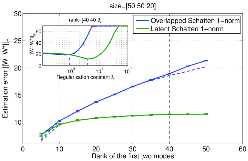
Figure 2: Estimation of a low-rank 50$\times$50$\times$20 tensor of rank $r\times r\times 3$ from noisy measurements. The noise standard deviation is $\sigma=0.1$. The estimation errors of two convex optimization based methods are plotted against the rank $r$ of the first two modes. The solid lines show the error at the fixed regularization constant $\lambda$, which is 0.89 for the overlapped approach and 3.79 for the latent approach (see also Figure 3). The dashed lines show the minimum error over candidates of the regularization constant $\lambda$ from 0.1 to 100. In the inset, the errors of the two approaches are plotted against the regularization constant $\lambda$ for rank $r=40$ (marked with gray dashed vertical line in the outset). The two values (0.89 and 3.79) are marked with vertical dashed lines. Note that both approaches need no knowledge of the true rank; the rank is automatically learned.

However, there are two issues that are not properly addressed so far.

The first issue is the statistical performance of the latent approach. In this paper, we show that the mean squared error of the latent approach scales no greater than the minimum mode-$k$ rank of the underlying true tensor, which clearly explains why the latent approach suffers less than the overlapped approach in Figure 2.

The second issue is the identifiability of the model underlying the latent approach, i.e., a mixture of low-rank tensors. In this paper, we show that such a mixture is identifiable only when the mixture consists of one component; in other words, when the underlying tensor is low-rank in a specific mode.

Along the way, we show a novel duality between the two types of norms employed in the above two approaches, namely the overlapped Schatten norm and the latent Schatten norm. This result is closely related and generalize the results in structured sparsity literature (Bach et al., 2011; Jenatton et al., 2011; Obozinski et al., 2011; Maurer & Pontil, 2011). In fact, the (plain) overlapped group lasso constrains the weights to be simultaneously group sparse over overlapping groups. The latent group lasso predicts with a mixture of group sparse weights (see also Wright et al., 2010; Jalali et al., 2010; Agarwal et al., 2011). These approaches clearly correspond to the two variations of tensor decomposition algorithms we discussed above.

Finally we empirically compare the overlapped approach and latent approach and show that even when the unknown tensor is simultaneously low-rank, which is a favorable situation for the overlapped approach, the latent approach performs better in many cases. Thus we provide both theoretical and empirical evidence that for noisy tensor decomposition, the latent approach is preferable to the overlapped approach. Our result is complementary to the previous study (Tomioka et al., 2011a, b), which mainly focused on the noise-less tensor completion setting.

This paper is structured as follows. In Section 2, we provide basic definitions of the two variations of structured Schatten norms, namely the overlapped/latent Schatten norms, and discuss their properties, especially the duality between them. Section 3 presents our main theoretical contributions; we establish the consistency of the latent approach, we show a denoising performance bound, and discuss the identifiability of the model underlying it. In Section 4, we empirically confirm the scaling predicted by our theory. Finally, Section 5 concludes the paper.

2 Structured Schatten norms for tensors

In this section, we define the overlapped Schatten norm and the latent Schatten norm and discuss their basic properties.

First we need some basic definitions.

Let $\mathcal{W}\in\mathbb{R}^{n_{1}\times\cdots n_{K}}$ be a $K$-way tensor. We denote the total number of entries in $\mathcal{W}$ by $N=\prod_{k=1}^{K}n_{k}$. The dot product between two tensors $\mathcal{W}$ and $\mathcal{X}$ is defined as $\left\langle\mathcal{W},\mathcal{X}\right\rangle={\rm vec}(\mathcal{W}){}^{\top}{\rm vec}(\mathcal{X})$; i.e., the dot product as vectors in $\mathbb{R}^{N}$. The Frobenius norm of a tensor is defined as $\bigl{|}\!\bigl{|}\!\bigl{|}\mathcal{W}\bigr{|}\!\bigr{|}\!\bigr{|}_{F}=\sqrt{\left\langle\mathcal{W},\mathcal{W}\right\rangle}$. Each dimensionality of a tensor is called a mode. The mode $k$ unfolding $\boldsymbol{W}_{(k)}\in\mathbb{R}^{n_{k}\times N/n_{k}}$ is a matrix that is obtained by concatenating the mode-$k$ fibers along columns; here a mode-$k$ fiber is an $n_{k}$ dimensional vector obtained by fixing all the indices but the $k$th index of $\mathcal{W}$. The mode-$k$ rank $\underline{r}_{k}$ of $\mathcal{W}$ is the rank of the mode-$k$ unfolding $\boldsymbol{X}_{(k)}$. We say that a tensor $\mathcal{W}$ has Tucker rank $(\underline{r}_{1},\ldots,\underline{r}_{K})$ if the mode-$k$ rank is $\underline{r}_{k}$ for $k=1,\ldots,K$ (Kolda & Bader, 2009). The mode $k$ folding is the inverse of the unfolding operation.

2.1 Overlapped Schatten norms

The low-rank inducing norm studied in (Signoretto et al., 2010; Gandy et al., 2011; Liu et al., 2009; Tomioka et al., 2011a), which we call overlapped Schatten 1-norm, can be written as follows:

$$\bigl{|}\!\bigl{|}\!\bigl{|}\mathcal{W}\bigr{|}\!\bigr{|}\!\bigr{|}_{\underline{S_{1}/1}} =\sum\nolimits_{k=1}^{K}\|\boldsymbol{W}_{(k)}\|_{S_{1}}.$$ (1)

In this paper, we consider the following more general overlapped $S_{p}/q$-norm, which includes the Schatten 1-norm as the special case $(p,q)=(1,1)$. The overlapped $S_{p}/q$-norm is written as follows:

$$\bigl{|}\!\bigl{|}\!\bigl{|}\mathcal{W}\bigr{|}\!\bigr{|}\!\bigr{|}_{\underline{S_{p}/q}} =\Bigl{(}\sum\nolimits_{k=1}^{K}\|\boldsymbol{W}_{(k)}\|_{S_{p}}^{q}\Bigr{)}^{1/q},$$ (2)

where $1\leq p,q\leq\infty$; here

$$\|\boldsymbol{W}\|_{S_{p}}=\Bigl{(}\sum\nolimits_{j=1}^{r}\sigma_{j}^{p}(\boldsymbol{W})\Bigr{)}^{1/p}$$

is the Schatten $p$-norm for matrices, where $\sigma_{j}(\boldsymbol{W})$ is the $j$th largest singular value of $\boldsymbol{W}$.

When used as a regularizer, the overlapped Schatten 1-norm penalizes all modes of $\mathcal{W}$ to be jointly low-rank. It is related to the overlapped group regularization (see Jenatton et al., 2011; Mairal et al., 2011) in a sense that the same object $\mathcal{W}$ appears repeatedly in the norm.

The following inequality relates the overlapped Schatten 1-norm with the Frobenius norm, which was a key step in the analysis of Tomioka et al. (2011b):

$$\bigl{|}\!\bigl{|}\!\bigl{|}\mathcal{W}\bigr{|}\!\bigr{|}\!\bigr{|}_{\underline{S_{1}/1}} \leq\sum_{k=1}^{K}\sqrt{\underline{r}_{k}}\bigl{|}\!\bigl{|}\!\bigl{|}\mathcal{W}\bigr{|}\!\bigr{|}\!\bigr{|}_{F},$$ (3)

where $\underline{r}_{k}$ is the mode-$k$ rank of $\mathcal{W}$.

Now we are interested in the dual norm of the overlapped $S_{p}/q$-norm, because deriving the dual norm is a key step in solving the minimization problem that involves the norm (2) (see Mairal et al., 2011), as well as computing various complexity measures, such as, Rademacher complexity (Foygel & Srebro, 2011) and Gaussian width (Chandrasekaran et al., 2010). It turns out that the dual norm of the overlapped $S_{p}/q$-norm is the latent $S_{p^{\ast}}/q^{\ast}$-norm as shown in the following lemma.

Lemma 1.

The dual norm of the overlapped $S_{p}/q$-norm is the latent $S_{p^{\ast}}/q^{\ast}$-norm, where $1/p+1/p^{\ast}=1$ and $1/q+1/q^{\ast}=1$, which is defined as follows:

$$\bigl{|}\!\bigl{|}\!\bigl{|}\mathcal{X}\bigr{|}\!\bigr{|}\!\bigr{|}_{\overline{S_{p^{\ast}}/q^{\ast}}}=\inf_{\left(\mathcal{X}^{(1)}+\cdots+\mathcal{X}^{(K)}\right)=\mathcal{X}} \left(\sum\nolimits_{k=1}^{K}\|\boldsymbol{X}_{(k)}^{(k)}\|_{S_{p^{\ast}}}^{q^{\ast}}\right)^{1/q^{\ast}}.$$ (4)

Here the infimum is taken over the $K$-tuple of tensors $\mathcal{X}^{(1)},\ldots,\mathcal{X}^{(K)}$ that sums to $\mathcal{X}$.

Proof.

The proof is presented in Appendix A. ∎

The duality in the above lemma naturally generalizes the duality between overlapped/latent group sparsity norms that have only partial overlap (in contrast to the complete overlap here). Although being recognized in special instances (Jalali et al., 2010; Obozinski et al., 2011; Maurer & Pontil, 2011; Agarwal et al., 2011), to the best of our knowledge, this duality has not been presented in the generality of Lemma 1. Note that when the groups have no overlap, the overlapped/latent group sparsity norms become identical, and the duality is the ordinary duality between the group $S_{p}/q$-norms and the group $S_{p^{\ast}}/q^{\ast}$-norms.

2.2 Latent Schatten norms

The latent approach for tensor decomposition proposed by Tomioka et al. (2011a) solves the following minimization problem

$$\mathop{\rm minimize}_{\mathcal{W}^{(1)},\ldots,\mathcal{W}^{(K)}}\quad L(\mathcal{W}^{(1)}+\cdots+\mathcal{W}^{(K)})+\lambda\sum_{k=1}^{K}\|\boldsymbol{W}_{(k)}^{(k)}\|_{S_{1}},$$ (5)

where $L$ is a loss function, $\lambda$ is a regularization constant, and $\boldsymbol{W}^{(k)}_{(k)}$ is the mode-$k$ unfolding of $\mathcal{W}^{(k)}$. Intuitively speaking, the latent approach for tensor decomposition predicts with a mixture of $K$ tensors that each are regularized to be low-rank in a specific mode.

Now, since the loss term in the minimization problem (5) only depends on the sum of the tensors $\mathcal{W}^{(1)},\ldots,\mathcal{W}^{(K)}$, minimization problem (5) is equivalent to the following minimization problem

$$\mathop{\rm minimize}_{\mathcal{W}}\quad L(\mathcal{W})+\lambda\bigl{|}\!\bigl{|}\!\bigl{|}\mathcal{W}\bigr{|}\!\bigr{|}\!\bigr{|}_{\overline{S_{1}/1}}.$$

In other words, we have identified the structured Schatten norm employed in the latent approach as the latent $S_{1}/1$-norm (or latent Schatten 1-norm for short), which can be written as follows:

$$\bigl{|}\!\bigl{|}\!\bigl{|}\mathcal{W}\bigr{|}\!\bigr{|}\!\bigr{|}_{\overline{S_{1}/1}}=\inf_{\left(\mathcal{W}^{(1)}+\cdots+\mathcal{W}^{(K)}\right)=\mathcal{W}}\sum_{k=1}^{K}\|\boldsymbol{W}_{(k)}^{(k)}\|_{S_{1}}.$$ (6)

According to Lemma 1, the dual norm of the latent $S_{1}/1$-norm is the overlapped $S_{\infty}/\infty$-norm

$$\bigl{|}\!\bigl{|}\!\bigl{|}\mathcal{X}\bigr{|}\!\bigr{|}\!\bigr{|}_{\underline{S_{\infty}/\infty}}=\max_{k}\|\boldsymbol{X}_{(k)}\|_{S_{\infty}},$$ (7)

where $\|\cdot\|_{S_{\infty}}$ is the spectral norm.

The following lemma is similar to inequality (3) and is a key in our analysis.

Lemma 2.

$$\bigl{|}\!\bigl{|}\!\bigl{|}\mathcal{W}\bigr{|}\!\bigr{|}\!\bigr{|}_{\overline{S_{1}/1}} \leq\left(\min_{k}\sqrt{\underline{r}_{k}}\right)\bigl{|}\!\bigl{|}\!\bigl{|}\mathcal{W}\bigr{|}\!\bigr{|}\!\bigr{|}_{F},$$

where $\underline{r}_{k}$ is the mode-$k$ rank of $\mathcal{W}$.

Proof.

Since we are allowed to take a singleton decomposition $\mathcal{W}^{(k)}=\mathcal{W}$ and $\mathcal{W}^{(k^{\prime})}=0$ $(k^{\prime}\neq k)$, we have

$$\bigl{|}\!\bigl{|}\!\bigl{|}\mathcal{W}\bigr{|}\!\bigr{|}\!\bigr{|}_{\overline{S_{1}/1}} =\inf_{\left(\mathcal{W}^{(1)}+\cdots+\mathcal{W}^{(K)}\right)=\mathcal{W}}\sum_{k=1}^{K}\|\boldsymbol{W}_{(k)}^{(k)}\|_{S_{1}}$$

$$\leq\|\boldsymbol{W}_{(k)}\|_{S_{1}}$$

$$\leq\sqrt{\underline{r}}_{k}\|\boldsymbol{W}_{(k)}\|\quad(\forall k=1,\ldots,K)$$

Choosing $k$ that minimizes the right hand side, we obtain our claim. ∎

Compared to inequality (3), the latent Schatten 1-norm is bounded by the minimal square root of the ranks instead of the sum. This is the fundamental reason why the latent approach performs betters than the overlapped approach as in Figure 2.

3 Main theoretical results

In this section, we study the consistency, generalization performance, and identifiability of the latent approach for tensor decomposition in the context of recovering an unknown tensor $\mathcal{W}^{\ast}$ from noisy measurements. This is the setting of the experiment in Figure 2.

First, we show that the latent approach is consistent. That is, the error goes to zero when the noise goes to zero, which corresponds to the situation when the entries are repeatedly observed.

Second, combining the duality we presented in the previous section with the techniques from Agarwal et al. (2011), we analyze the denoising performance of the latent approach in the context of recovering an unknown tensor $\mathcal{W}^{\ast}$ from noisy measurements. This is the setting of the experiment in Figure 2. We first prove a deterministic inequality that holds under certain condition on the regularization constant. Next, we assume Gaussian noise and derive an inequality that holds with high probability under an appropriate scaling of the regularization constant.

Third, we discuss the difference between overlapped approach and latent approach and provide an explanation for the empirically observed superior performance of the latent approach in Figure 2.

Finally we discuss the condition under which the decomposition $\mathcal{W}=\sum_{k=1}^{K}\mathcal{W}^{(k)}$ is identifiable and show that the model is (locally) identifiable only when the mixture consists of one component.

3.1 Consistency

Let $\mathcal{W}^{\ast}$ be the underlying true tensor and the noisy version $\mathcal{Y}$ is obtained as follows:

$$\mathcal{Y} =\mathcal{W}^{\ast}+\mathcal{E},$$

where $\mathcal{E}\in\mathbb{R}^{n_{1}\times\cdots\times n_{K}}$ is the noise tensor.

First we establish the consistency of the latent approach.

Theorem 1.

The estimator defined by

$$\hat{\mathcal{W}}=\mathop{\rm argmin}_{\mathcal{W}}\Biggl{(}\frac{1}{2} \bigl{|}\!\bigl{|}\!\bigl{|}\mathcal{Y}-\mathcal{W}\bigr{|}\!\bigr{|}\!\bigr{|}_{F}^{2}+\lambda\bigl{|}\!\bigl{|}\!\bigl{|}\mathcal{W}\bigr{|}\!\bigr{|}\!\bigr{|}_{\overline{S_{1}/1}}\Biggr{)},$$ (8)

is consistent. That is, when the noise goes to zero (e.g., when the entries are repeatedly observed), $\hat{\mathcal{W}}\rightarrow\mathcal{W}^{\ast}$ for any sequence $\lambda\rightarrow 0$.

Proof.

Due to the triangular inequality

$$\bigl{|}\!\bigl{|}\!\bigl{|}\hat{\mathcal{W}}-\mathcal{W}^{\ast}\bigr{|}\!\bigr{|}\!\bigr{|}_{F} \leq\bigl{|}\!\bigl{|}\!\bigl{|}\hat{\mathcal{W}}-\mathcal{Y}\bigr{|}\!\bigr{|}\!\bigr{|}_{F}+\bigl{|}\!\bigl{|}\!\bigl{|}\mathcal{Y}-\mathcal{W}^{\ast}\bigr{|}\!\bigr{|}\!\bigr{|}_{F}.$$

Here the second term goes to zero as the noise shrinks. Next, from the optimality of $\hat{\mathcal{W}}$, the first term satisfies

$$\mathcal{Y}-\hat{\mathcal{W}} \in\lambda\partial\bigl{|}\!\bigl{|}\!\bigl{|}\hat{\mathcal{W}}\bigr{|}\!\bigr{|}\!\bigr{|}_{\overline{S_{1}/1}},$$

where $\partial\bigl{|}\!\bigl{|}\!\bigl{|}\hat{\mathcal{W}}\bigr{|}\!\bigr{|}\!\bigr{|}_{\overline{S_{1}/1}}$ is the subdifferential of the latent $S_{1}/1$ norm at $\hat{\mathcal{W}}$. Now since the dual norm of the latent $S_{1}/1$ norm is the overlapped $S_{\infty}/\infty$ norm, for any $\mathcal{G}\in\partial\bigl{|}\!\bigl{|}\!\bigl{|}\hat{\mathcal{W}}\bigr{|}\!\bigr{|}\!\bigr{|}_{\overline{S_{1}/1}}$, we have $\bigl{|}\!\bigl{|}\!\bigl{|}\mathcal{G}\bigr{|}\!\bigr{|}\!\bigr{|}_{\underline{S_{\infty}/\infty}}\leq 1$, and therefore

$$\bigl{|}\!\bigl{|}\!\bigl{|}\hat{\mathcal{W}}-\mathcal{Y}\bigr{|}\!\bigr{|}\!\bigr{|}_{F} \leq C\bigl{|}\!\bigl{|}\!\bigl{|}\hat{\mathcal{W}}-\mathcal{Y}\bigr{|}\!\bigr{|}\!\bigr{|}_{\underline{S_{\infty}/\infty}}\leq C\lambda,$$

where $C$ is a constant that is independent of $\lambda$. Therefore, for any sequence $\lambda\rightarrow 0$, we have $\hat{\mathcal{W}}\rightarrow\mathcal{W}^{\ast}$ when $\mathcal{E}\rightarrow 0$. ∎

3.2 Deterministic bound

The consistency statement in the previous section only deals with the sum $\hat{\mathcal{W}}=\sum_{k=1}^{K}\hat{\mathcal{W}}^{(k)}$ and its convergence to the truth $\mathcal{W}^{\ast}$ in the limit the noise goes to zero. In this section, we establish a stronger statement that shows the behavior of individual terms $\hat{\mathcal{W}}^{(k)}$ and also the denoising performance.

To this end we need some additional assumptions.

First, we assume that the unknown tensor $\mathcal{W}^{\ast}$ is a mixture of $K$ tensors that each are low-rank in a certain mode and we have a noisy observation $\mathcal{Y}$ as follows:

$$\mathcal{Y}=\mathcal{W}^{\ast}+\mathcal{E}=\sum\nolimits_{k=1}^{K}\mathcal{W}^{\ast(k)}+\mathcal{E},$$ (9)

where $\bar{r}_{k}={\rm rank}(\boldsymbol{W}^{(k)}_{(k)})$ is the mode-$k$ rank of the $k$th component $\mathcal{W}^{\ast(k)}$.

Second, we assume that the spectral norm of the mode-$k$ unfolding of the $l$th component is bounded by a constant $\alpha$ for all $k\neq l$ as follows:

$$\|\boldsymbol{W}_{(k)}^{\ast(l)}\|_{S_{\infty}} \leq\alpha\quad(\forall l\neq k,k,l=1,\ldots,K).$$ (10)

Note that such an additional incoherence assumption has also been used in (Candes et al., 2009; Wright et al., 2010; Agarwal et al., 2011; Hsu et al., 2011).

We employ the following optimization problem to recover the unknown tensor $\mathcal{W}^{\ast}$:

$$\hat{\mathcal{W}}=\mathop{\rm argmin}_{\mathcal{W}}\Biggl{(}\frac{1}{2} \bigl{|}\!\bigl{|}\!\bigl{|}\mathcal{Y}-\mathcal{W}\bigr{|}\!\bigr{|}\!\bigr{|}_{F}^{2}+\lambda\bigl{|}\!\bigl{|}\!\bigl{|}\mathcal{W}\bigr{|}\!\bigr{|}\!\bigr{|}_{\overline{S_{1}/1}}$$

$$\quad{\rm s.t.}\quad\|\boldsymbol{W}^{(k)}_{(l)}\|_{S_{\infty}}\leq\alpha,\quad\forall l\neq k\Biggr{)},$$ (11)

where $\mathcal{W}=\sum_{k=1}^{K}\mathcal{W}^{(k)}$ denotes the optimal decomposition induced by the latent Schatten 1-norm (6); $\lambda>0$ is a regularization constant. Notice that we have introduced additional spectral norm constraints to control the correlation between the components (see also Agarwal et al., 2011).

Our first bound can be stated as follows:

Theorem 2.

Let $\hat{\mathcal{W}}^{(k)}$ be an optimal decomposition of $\hat{\mathcal{W}}$ induced by the latent Schatten 1-norm (6). Assume that the regularization constant $\lambda$ satisfies $\lambda\geq 2\bigl{|}\!\bigl{|}\!\bigl{|}\mathcal{E}\bigr{|}\!\bigr{|}\!\bigr{|}_{\underline{S_{\infty}/\infty}}+\alpha(K-1)$. Then there is a universal constant $c$ such that, any solution $\hat{\mathcal{W}}$ of the minimization problem (3.2) satisfies the following deterministic bound:

$$\sum_{k=1}^{K}\bigl{|}\!\bigl{|}\!\bigl{|}\hat{\mathcal{W}}^{(k)}-\mathcal{W}^{\ast(k)}\bigr{|}\!\bigr{|}\!\bigr{|}_{F}^{2} \leq c\lambda^{2}\sum_{k=1}^{K}\overline{r}_{k}.$$ (12)

Proof.

The proof is presented in Appendix B. ∎

We can also obtain a bound on the difference of the whole tensor $\hat{\mathcal{W}}-\mathcal{W}^{\ast}$ rather than the squared sum differences as in Theorem 2 as follows.

Corollary 1.

Under the same conditions as in Theorem 2 we have

$$\bigl{|}\!\bigl{|}\!\bigl{|}\hat{\mathcal{W}}-\mathcal{W}^{\ast}\bigr{|}\!\bigr{|}\!\bigr{|}_{F}^{2} \leq cK\lambda^{2}\sum_{k=1}^{K}\bar{r}_{k}.$$ (13)

Proof.

Using the triangular inequality and Cauchy-Schwarz inequality we have $\bigl{|}\!\bigl{|}\!\bigl{|}\hat{\mathcal{W}}-\mathcal{W}^{\ast}\bigr{|}\!\bigr{|}\!\bigr{|}_{F}\leq\sum_{k=1}^{K}\bigl{|}\!\bigl{|}\!\bigl{|}\hat{\mathcal{W}}^{(k)}-\mathcal{W}^{\ast(k)}\bigr{|}\!\bigr{|}\!\bigr{|}_{F}\leq\sqrt{K}\sqrt{\sum_{k=1}^{K}\bigl{|}\!\bigl{|}\!\bigl{|}\hat{\mathcal{W}}^{(k)}-\mathcal{W}^{\ast(k)}\bigr{|}\!\bigr{|}\!\bigr{|}_{F}^{2}}$. ∎

Since we are bounding the overall error in (13), we may exploit the arbitrariness of the decomposition $\mathcal{W}^{\ast}=\sum_{k=1}^{K}\mathcal{W}^{\ast(k)}$ to obtain a tight bound. The tightest bound is obtained when we choose the decomposition that minimizes the sum of the ranks $\sum_{k=1}^{K}\bar{r}_{k}$. We say $\mathcal{W}^{\ast}$ has the latent rank $(\overline{r}_{1},\ldots,\overline{r}_{K})$ for such a minimal decomposition in terms of the sum.

A simple upper bound is obtained by choosing a decomposition $\mathcal{W}^{\ast(k)}=\mathcal{W}^{\ast}$ and $\mathcal{W}^{\ast(k^{\prime})}=0$ for $k^{\prime}\neq k$. In particular by choosing the mode with the minimum mode-$k$ rank, we obtain

$$\bigl{|}\!\bigl{|}\!\bigl{|}\hat{\mathcal{W}}-\mathcal{W}^{\ast}\bigr{|}\!\bigr{|}\!\bigr{|}_{F}^{2}\leq cK\lambda^{2}\min_{k=1,\ldots,K}\underline{r}_{k},$$

where $\underline{r}_{k}$ is the mode-$k$ rank of $\mathcal{W}^{\ast}$. We refer to the above decomposition as the minimum rank singleton decomposition.

Note that the right-hand side of our bound (12) does not necessarily go to zero when the noise $\mathcal{E}$ goes to zero, because $\lambda\geq\alpha(K-1)$. When the noise goes to zero, $\hat{\mathcal{W}}\rightarrow\mathcal{W}^{\ast}$ can be obtained by any decreasing sequence $\lambda\rightarrow 0$ as shown in the previous subsection. Therefore our bound is most useful when the noise is relatively large and the first term $2\bigl{|}\!\bigl{|}\!\bigl{|}\mathcal{E}\bigr{|}\!\bigr{|}\!\bigr{|}_{\underline{S_{\infty}}/\infty}$ dominates the second term $\alpha(K-1)$ in the condition for the regularization constant $\lambda$.

3.3 Gaussian noise

When the elements of the noise tensor $\mathcal{E}$ are Gaussian, we obtain the following theorem.

Theorem 3.

Assume that the elements of the noise tensor $\mathcal{E}$ are independent Gaussian random variables with variance $\sigma^{2}$. In addition, assume without loss of generality that the dimensionalities of $\mathcal{W}^{\ast}$ are sorted in the descending order, i.e., $n_{1}\geq\cdots\geq n_{K}$. Then there are universal constants $c_{0},c_{1}$ such that, with high probability, any solution of the minimization problem (3.2) with regularization constant $\lambda=c_{0}\sigma(\sqrt{N/n_{K}}+\sqrt{n_{1}}+\sqrt{\log K})+\alpha(K-1)$ satisfies the following bound:

$$\frac{1}{N}\sum_{k=1}^{K}\bigl{|}\!\bigl{|}\!\bigl{|}\hat{\mathcal{W}}^{(k)}-\mathcal{W}^{\ast(k)}\bigr{|}\!\bigr{|}\!\bigr{|}_{F}^{2} \leq c_{1}F\sigma^{2}\frac{\sum_{k=1}^{K}\bar{r}_{k}}{n_{K}},$$ (14)

where $F=\left(\left(1+\sqrt{\frac{n_{1}n_{K}}{N}}\right)+\left(\sqrt{\log K}+\frac{\alpha(K-1)}{c_{0}\sigma}\right)\sqrt{\frac{n_{K}}{N}}\right)^{2}$ is a factor that mildly depends on the dimensionalities and the constant $\alpha$ in (10).

Proof.

The proof is presented in Appendix C ∎

Note that the theoretically optimal choice of regularization constant $\lambda$ is independent of the Tucker/latent rank of the truth $\mathcal{W}^{\ast}$, which is unknown in practice.

Again we can obtain a bound corresponding to the minimum rank singleton decomposition as in inequality (13) as follows:

$$\frac{1}{N}\bigl{|}\!\bigl{|}\!\bigl{|}\hat{\mathcal{W}}-\mathcal{W}^{\ast}\bigr{|}\!\bigr{|}\!\bigr{|}_{F}^{2} \leq c_{1}KF\sigma^{2}\frac{\min_{k}\underline{r}_{k}}{n_{K}},$$ (15)

where $F$ is the same factor as in Theorem 3.

3.4 Comparison with the overlapped approach

Inequality (15) explains the superior performance of the latent approach for tensor decomposition in Figure 2. The inequality obtained in (Tomioka et al., 2011b) for the overlapped approach that uses overlapped Schatten 1-norm (1) can be stated as follows:

$$\frac{1}{N}\bigl{|}\!\bigl{|}\!\bigl{|}\hat{\mathcal{W}}-\mathcal{W}^{\ast}\bigr{|}\!\bigr{|}\!\bigr{|}_{F}^{2} \leq c_{1}^{\prime}\sigma^{2}\!\!\left(\frac{1}{K}\sum_{k=1}^{K}\sqrt{\textstyle\frac{1}{n_{k}}}\right)^{2}\!\!\left(\frac{1}{K}\sum_{k=1}^{K}\sqrt{\underline{r}_{k}}\right)^{2}.$$ (16)

Comparing inequalities (15) and (16), we notice that the complexity of the overlapped approach depends on the average (square root) of the Tucker rank $\underline{r}_{1},\ldots,\underline{r}_{K}$, whereas that of the latent approach only grows linearly against the minimum Tucker rank. Interestingly, the latent approach performs as if it knows the mode with the minimum rank, although such information is not available to it. However in inequality (15) we have the factor $K$. This means that if the mode with the minimum rank is known, the latent approach looses by constant factor $K$ against the simple matrix decomposition approach that unfolds the given tensor at the minimal rank mode and performs ordinary Schatten 1-norm minimization.

3.5 Discussion on the identifiability

Let $\bar{r}_{k}={\rm rank}(\boldsymbol{W}^{(k)}_{(k)})$ be the mode-$k$ rank of the $k$th component $\mathcal{W}^{(k)}$ in the decomposition

$$\mathcal{W} =\mathcal{W}^{(1)}+\mathcal{W}^{(2)}+\cdots+\mathcal{W}^{(K)}.$$ (17)

We say that a decomposition (17) is locally identifiable when there is no other decomposition $\sum_{k=1}^{K}\tilde{\mathcal{W}}^{(k)}$ having the same rank $(\bar{r}_{1},\ldots,\bar{r}_{K})$. The following theorem fully characterizes the local identifiability of the decomposition (17).

Theorem 4.

The decomposition (17) is locally identifiable if and only if $\mathcal{W}^{(k^{\ast})}=\mathcal{W}$ for $k=k^{\ast}$ and $\mathcal{W}^{(k)}=0$ otherwise, for some $k^{\ast}$.

Proof.

The proof is given in Appendix D. ∎

The above theorem partly explains the difficulty of estimating individual components $\mathcal{W}^{\ast(k)}$ without additional incoherence assumption as in (10). In fact, most decompositions of the form (9) are not identifiable.

4 Numerical results

In this section, we numerically confirm the scaling behavior we have theoretically predicted in the last section.

The goal of this experiment is to recover the true low rank tensor $\mathcal{W}^{\ast}$ from a noisy observation $\mathcal{Y}$. We randomly generated the true low rank tensors $\mathcal{W}^{\ast}$ of size $50\times 50\times 20$ or $80\times 80\times 40$ with various Tucker ranks $(\underline{r}_{1},\underline{r}_{2},\underline{r}_{3})$. A low-rank tensor is generated by first randomly drawing the $\underline{r}_{1}\times\underline{r}_{2}\times\underline{r}_{3}$ core tensor from the standard normal distribution and multiplying an orthogonal factor matrix drawn from the Haar measure to its each mode. The observation tensor $\mathcal{Y}$ is obtained by adding Gaussian noise with standard deviation $\sigma=0.1$. There is no missing entries in this experiment.

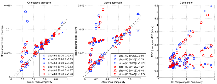
Figure 3: Performance of the overlapped approach and latent approach for tensor decomposition are shown against their theoretically predicted complexity measures (see Eqs. (18) and (19)). The right panel shows the improvement of the latent approach from the overlapped approach against the ratio of their complexity measures.

For an observation $\mathcal{Y}$, we computed tensor decompositions using the overlapped approach and the latent approach (3.2) using the solver available from the webpage of one of the authors of Tomioka et al. (2011a). The solver uses the alternating direction method of multipliers (Gabay & Mercier, 1976) and the algorithm is described in the above paper. We computed the solutions for 20 candidate regularization constants ranging from 0.1 to 100 and report the results for three representative values for each method.

We measured the quality of the solutions obtained by the two approaches by the mean squared error (MSE) $\bigl{|}\!\bigl{|}\!\bigl{|}\hat{\mathcal{W}}-\mathcal{W}^{\ast}\bigr{|}\!\bigr{|}\!\bigr{|}_{F}^{2}/N$. In order to make our theoretical predictions more concrete, we define the quantities in the right hand side of the bounds (16) and (14) as Tucker rank (TR) complexity and Latent rank (LR) complexity, respectively, as follows:

TR complexity $$=\left(\textstyle\frac{1}{K}\sum\nolimits_{k=1}^{K}\sqrt{\textstyle\frac{1}{n_{k}}}\right)^{2}\left(\textstyle\frac{1}{K}\sum\nolimits_{k=1}^{K}\sqrt{\underline{r}_{k}}\right)^{2},$$ (18)

LR complexity $$=\frac{\sum_{k=1}^{K}\bar{r}_{k}}{n_{K}},$$ (19)

where without loss of generality we assume $n_{1}\geq\cdots\geq n_{K}$. We have ignored terms like $\sqrt{n_{k}/N}$ because they are negligible for $n_{k}\approx 50$ and $N\approx 50,000$. The TR complexity is equivalent to the normalized rank in (Tomioka et al., 2011b). Note that the TR complexity (18) is defined in terms of the Tucker rank $(\underline{r}_{1},\ldots,\underline{r}_{K})$ of the truth $\mathcal{W}^{\ast}$, whereas the LR complexity (19) is defined in terms of the latent rank $(\overline{r}_{1},\ldots,\overline{r}_{K})$ (see Section 3.2). In order to compute the sum of latent ranks $\sum_{k=1}^{K}\overline{r}_{k}$, we ran the latent approach to the true tensor $\mathcal{W}^{\ast}$ without noise, and took the minimum of the sums obtained from that and the minimum rank singleton decomposition. The whole procedure is repeated 10 times and averaged.

Figure 3 shows the results of the experiment. The left panel shows the MSE of the overlapped approach against the TR complexity (18). The middle panel shows the MSE of the latent approach against the LR complexity (19). The right panel shows the improvement (i.e., MSE of the overlap approach divided by that of the latent approach) against the ratio of the respective complexity measures.

First, from the left panel we can confirm that as predicted by (Tomioka et al., 2011b), the MSE of the overlapped approach scales linearly against the TR complexity (18) for each value of the regularization constant. We can also see that as predicted by Theorem 3, by scaling the regularization constant proportionally with $\sqrt{N/n_{K}}$, the series corresponding to size $50\times 50\times 20$ and those corresponding to size $80\times 80\times 40$ almost lie on top of each others.

From the central panel, we can clearly see that the MSE of the latent approach scales linearly against the LR complexity (19) as predicted by Theorem 3. The series with $\bigtriangleup$ ($\lambda=3.79$ for $50\times 50\times 20$, $\lambda=5.46$ for $80\times 80\times 40$) is mostly below other series, which means that the optimal choice of the regularization constant is independent of the rank of the true tensor and only depends on the size; this agrees with the condition on $\lambda$ in Theorem 3. Since the blue series and red series with the same markers lie on top of each other (especially the series with $\bigtriangleup$ for which the optimal regularization constant is chosen), we can see that our theory predicts not only the scaling against the latent ranks but also that against the size of the tensor correctly. Note that the regularization constants are scaled by roughly 1.6 to account for the difference in the dimensionality.

The right panel reveals that in many cases the latent approach performs better than the overlapped approach, i.e., MSE (overlap)/ MSE (latent) greater than one. Moreover, we can see that the success of the latent approach relative to the overlapped approach is correlated with high TR complexity to LR complexity ratio. Indeed, we found that the optimal decomposition of the true tensor $\mathcal{W}^{\ast}$ was typically a singleton decomposition corresponding to the smallest tucker rank (see Section 3.2).

One might think that we can fix the overlapped approach by allowing individual regularization constant for each mode. However, this would only be possible if we knew the mode with small rank.

The improvements here are milder than that in Figure 2. This is because most of the randomly generated low-rank tensors were simultaneously low-rank to some degree. It is interesting that the latent approach perform at least as good as the overlapped approach also in such situations.

5 Conclusion

In this paper, we have presented a framework for structured Schatten norms. The current framework includes both the overlapped Schatten 1-norm and latent Schatten 1-norm recently proposed in the context of convex-optimization-based tensor decomposition (Signoretto et al., 2010; Gandy et al., 2011; Liu et al., 2009; Tomioka et al., 2011a), and connects these studies to the broader studies on structured sparsity (Bach et al., 2011; Jenatton et al., 2011; Obozinski et al., 2011; Maurer & Pontil, 2011). Moreover, we have shown a duality that holds between the two types of norms.

Furthermore, we have rigorously studied the performance of the latent approach for tensor decomposition. We have shown the consistency of the latent Schatten 1-norm minimization. Next, we have analyzed the denoising performance of the latent approach and shown that the error of the latent approach is upper bounded by the minimum Tucker rank, which contrasts sharply against the average (square root) dependency of the overlapped approach analyzed in Tomioka et al. (2011b). This explains the empirically observed superior performance of the latent approach compared to the overlapped approach. The most difficult case for the overlapped approach is when the unknown tensor is only low-rank in one mode as in Figure 2.

We have also confirmed through numerical simulations that our analysis precisely predicts the scaling of the mean squared error as a function of the dimensionalities and the latent rank of the unknown tensor. Unlike Tucker rank, latent rank of a tensor is not easy to compute. However, note that the theoretically optimal scaling of the regularization constant does not depend on the latent rank.

Therefore we have theoretically and empirically shown that for noisy tensor decomposition, the latent approach is more likely to perform better than the overlapped approach. Analyzing the performance of the latent approach for tensor completion would be an important future work.

The structured Schatten norms proposed in this paper include norms for tensors that are not employed in practice yet. Therefore, we envision that this paper serve as a starting point for various extensions, e.g., using the overlapped $S_{1}/\infty$-norm instead of the $S_{1}/1$-norm or a non-sparse tensor decomposition similar to the $\ell_{p}$-norm MKL (Micchelli & Pontil, 2005; Kloft et al., 2011).

Supplementary material for “Convex Tensor Decomposition via Structured Schatten Norms”

Appendix A Proof of Lemma 1

Proof.

From the definition, the dual norm $\bigl{|}\!\bigl{|}\!\bigl{|}\mathcal{X}\bigr{|}\!\bigr{|}\!\bigr{|}_{(\underline{S_{p}/q})^{\ast}}$ can be written as follows:

$$\bigl{|}\!\bigl{|}\!\bigl{|}\mathcal{W}\bigr{|}\!\bigr{|}\!\bigr{|}_{(\underline{S_{p}/q})^{\ast}}=\sup\left\langle\mathcal{W},\mathcal{X}\right\rangle\quad{\rm s.t.}\quad\bigl{|}\!\bigl{|}\!\bigl{|}\mathcal{W}\bigr{|}\!\bigr{|}\!\bigr{|}_{\underline{S_{p}/q}}\leq 1.$$

The basic strategy of the proof is to rewrite the above maximization problem as a constraint optimization problem and derive the dual problem.

First, we rewrite the above maximization problem as follows:

$$\bigl{|}\!\bigl{|}\!\bigl{|}\mathcal{X}\bigr{|}\!\bigr{|}\!\bigr{|}_{(\underline{S_{p}/q})^{\ast}} =\sup\frac{1}{K}\sum_{k=1}^{K}\left\langle\boldsymbol{Z}_{k},\boldsymbol{X}_{(k)}\right\rangle$$

$${\rm s.t.}\quad\boldsymbol{Z}_{k}=\boldsymbol{W}_{(k)},\sum_{k=1}^{K}\|\boldsymbol{Z}_{k}\|_{S_{p}}^{q}\leq 1,$$

where $\boldsymbol{Z}_{k}\in\mathbb{R}^{n_{k}\times N/n_{k}}$ ($k=1,\ldots,K$) are auxiliary variables.

Next we write down the Lagrangian as follows:

$$L =\frac{1}{K}\sum_{k}\left\langle\boldsymbol{Z}_{k},\boldsymbol{X}_{(k)}\right\rangle$$

$$\qquad+\frac{1}{K}\sum_{k}\left\langle\tilde{\mathcal{Y}}^{(k)},\boldsymbol{Z}_{k}^{(k)}-\boldsymbol{W}\right\rangle$$

$$\qquad+\frac{\gamma}{Kq}\left(1-\sum\nolimits_{k}\|\boldsymbol{Z}_{k}\|_{S_{p}}^{q}\right),$$

where $\tilde{\mathcal{Y}}^{(k)}\in\mathbb{R}^{n_{1}\times\cdots\times n_{K}}$ ($k=1,\ldots,K$), and $\gamma\geq 0$ are Lagrangian multipliers.

Note that for $\boldsymbol{X},\boldsymbol{Z}\in\mathbb{R}^{R\times C}$, we have

$$\sup_{\boldsymbol{Z}}\left(\left\langle\boldsymbol{X},\boldsymbol{Z}\right\rangle-\frac{\gamma}{q}\|\boldsymbol{Z}\|_{S_{p}}^{q}\right)$$

$$\leq\gamma\sup_{\boldsymbol{Z}}\left(\|\boldsymbol{X}/\gamma\|_{S_{p^{\ast}}}\|\boldsymbol{Z}\|_{S_{p}}-\frac{1}{q}\|\boldsymbol{Z}\|_{S_{p}}^{q}\right)$$

$$\leq\frac{\gamma^{1-q^{\ast}}}{q^{\ast}}\|\boldsymbol{X}\|_{S_{p^{\ast}}}^{q^{\ast}}.$$

Here the first equality is achieved if we take $\boldsymbol{Z}=c\boldsymbol{U}{\rm diag}(\sigma_{1}^{p^{\ast}/p},\ldots,\sigma_{r}^{p^{\ast}/p})\boldsymbol{V}{}^{\top}$, where $\boldsymbol{U}{\rm diag}(\sigma_{1},\ldots,\sigma_{r})\boldsymbol{V}{}^{\top}$ is the singular value decomposition of the matrix $\boldsymbol{X}/\gamma$, and $c$ is an arbitrary scaling constant. The second equality is achieved if we take $\|\boldsymbol{Z}\|_{S_{p}}=\|\boldsymbol{X}/\gamma\|_{S_{p^{\ast}}}^{\frac{1}{q-1}}$.

Thus, maximizing the Lagrangian with respect to $\boldsymbol{Z}_{k}$ ($k=1,\ldots,K$) and $\mathcal{W}$, we obtain the dual problem

$$\bigl{|}\!\bigl{|}\!\bigl{|}\mathcal{X}\bigr{|}\!\bigr{|}\!\bigr{|}_{\left(S_{1}/q\right)^{\ast}} =\!\!\!\!\inf_{\gamma,\mathcal{Y}^{(1)},\ldots,\mathcal{Y}^{(K)}}\!\!\left(\frac{\gamma^{1-q^{\ast}}}{K^{1-q^{\ast}}q^{\ast}}\sum_{k=1}^{K}\|\boldsymbol{Y}_{(k)}^{(k)}\|_{S_{p^{\ast}}}^{q^{\ast}}+\frac{\gamma}{Kq}\right)$$

$${\rm s.t.}\quad \mathcal{Y}^{(1)}+\cdots+\mathcal{Y}^{(K)}=\mathcal{X},$$

where we used the change of variable $(\mathcal{X}+\tilde{\mathcal{Y}}^{(k)})/K=:\mathcal{Y}^{(k)}$. Furthermore, by explicitly minimizing over $\gamma$, we have $\gamma/K=(\sum_{k=1}^{K}\|\boldsymbol{Y}_{(k)}^{(k)}\|_{S_{p^{\ast}}}^{q^{\ast}})^{1/q^{\ast}}$ and we obtain the statement of the lemma. ∎

Appendix B Proof of Theorem 2

Let $\hat{\mathcal{W}}=\sum_{k=1}^{K}\hat{\mathcal{W}}^{(k)}$ be the solution and its optimal decomposition of the minimization problem (3.2); in addition let $\Delta^{(k)}:=\hat{\mathcal{W}}^{(k)}-\mathcal{W}^{\ast(k)}$.

The proof is based on Lemmas 3 and 4, which we present below.

In order to present the first lemma, we need the following definitions. Let $\boldsymbol{U}_{k}\boldsymbol{S}_{k}\boldsymbol{V}_{k}=\boldsymbol{W}^{\ast(k)}_{(k)}$ be the singular value decomposition of the mode-$k$ unfolding of the $k$th component of the unknown tensor $\mathcal{W}^{\ast}$. We define the orthogonal projection of $\Delta^{(k)}$ as follows:

$$\boldsymbol{\Delta}^{(k)}_{(k)} =\boldsymbol{\Delta}_{k}^{\prime}+\boldsymbol{\Delta}_{k}^{\prime\prime},$$

where

$$\boldsymbol{\Delta}_{k}^{\prime\prime} =(\boldsymbol{I}_{n_{k}}-\boldsymbol{U}_{k}\boldsymbol{U}_{k}{}^{\top})\boldsymbol{\Delta}_{(k)}^{(k)}(\boldsymbol{I}_{N/n_{k}}-\boldsymbol{V}_{k}\boldsymbol{V}_{k}{}^{\top}).$$

Intuitively speaking, $\boldsymbol{\Delta}_{k}^{\prime\prime}$ lies in a subspace completely orthogonal to the unfolding of the $k$th component $\boldsymbol{W}^{\ast(k)}_{(k)}$, whereas $\boldsymbol{\Delta}_{k}^{\prime}$ lies in a partially correlated subspace.

The following lemma is similar to Negahban et al. (2009, Lemma 1) and Tomioka et al. (2011b, Lemma 2), and it bounds the Schatten 1-norm of the orthogonal part $\boldsymbol{\Delta}_{k}^{\prime\prime}$ with that of the partially correlated part $\boldsymbol{\Delta}_{k}^{\prime}$ and also bounds the rank of $\boldsymbol{\Delta}_{k}^{\prime}$ .

Lemma 3.

Let $\hat{\mathcal{W}}$ be the solution of the minimization problem (3.2) with the regularization constant $\lambda\geq 2\bigl{|}\!\bigl{|}\!\bigl{|}\mathcal{E}\bigr{|}\!\bigr{|}\!\bigr{|}_{\underline{S_{\infty}/\infty}}$. Let $\Delta^{(k)}$ and its decomposition be as defined above. Then we have

1. ${\rm rank}(\boldsymbol{\Delta}_{k}^{\prime})\leq 2\bar{r}_{k}$.

2. $\sum_{k=1}^{K}\|\boldsymbol{\Delta}_{k}^{\prime\prime}\|_{S_{1}}\leq 3\sum_{k=1}^{K}\|\boldsymbol{\Delta}_{k}^{\prime}\|_{S_{1}}$.

Note that although the proof of the above statement closely follows that of Tomioka et al. (2011b, Lemma 2), the notion of rank is different. In their result, the rank is the Tucker rank $\underline{r}_{k}$, whereas the rank here is the mode-$k$ rank of the $k$th component $\mathcal{W}^{\ast(k)}$ of the truth.

The following lemma relates the squared Frobenius norm of the difference of the sums $\bigl{|}\!\bigl{|}\!\bigl{|}\sum_{k=1}^{K}\Delta^{(k)}\bigr{|}\!\bigr{|}\!\bigr{|}_{F}^{2}$ with the sum of squared differences $\sum_{k=1}^{K}\bigl{|}\!\bigl{|}\!\bigl{|}\Delta^{(k)}\bigr{|}\!\bigr{|}\!\bigr{|}_{F}^{2}$

Lemma 4.

Let $\hat{\mathcal{W}}$ be the solution of the minimization problem (3.2). Then we have,

$$\frac{1}{2}\sum_{k=1}^{K}\bigl{|}\!\bigl{|}\!\bigl{|}\Delta^{(k)}\bigr{|}\!\bigr{|}\!\bigr{|}_{F}^{2}\leq\frac{1}{2}\bigl{|}\!\bigl{|}\!\bigl{|}\Delta\bigr{|}\!\bigr{|}\!\bigr{|}_{F}^{2}+\alpha(K-1)\sum_{k=1}^{K}\|\boldsymbol{\Delta}_{(k)}^{(k)}\|_{S_{1}},$$

where $\Delta=\sum_{k=1}^{K}\Delta^{(k)}$.

Proof of Theorem 2..

First from the optimality of $\hat{\mathcal{W}}$, we have

$$\frac{1}{2}\bigl{|}\!\bigl{|}\!\bigl{|}\mathcal{Y}-\hat{\mathcal{W}}\bigr{|}\!\bigr{|}\!\bigr{|}_{F}^{2} +\lambda\sum\nolimits_{k=1}^{K}\|\hat{\boldsymbol{W}}^{(k)}_{(k)}\|_{S_{1}}$$

$$\leq\frac{1}{2}\bigl{|}\!\bigl{|}\!\bigl{|}\mathcal{Y}-\mathcal{W}^{\ast}\bigr{|}\!\bigr{|}\!\bigr{|}_{F}^{2}+\lambda\sum\nolimits_{k=1}^{K}\|\boldsymbol{W}^{\ast(k)}_{(k)}\|_{S_{1}},$$

which implies

$$\frac{1}{2}\bigl{|}\!\bigl{|}\!\bigl{|}\Delta\bigr{|}\!\bigr{|}\!\bigr{|}_{F}^{2} \leq\left\langle\Delta,\mathcal{E}\right\rangle+\lambda\sum\nolimits_{k=1}^{K}\|\boldsymbol{\Delta}_{(k)}^{(k)}\|_{S_{1}}$$

$$\leq(\bigl{|}\!\bigl{|}\!\bigl{|}\mathcal{E}\bigr{|}\!\bigr{|}\!\bigr{|}_{\underline{S_{\infty}/\infty}}+\lambda)\sum\nolimits_{k=1}^{K}\|\boldsymbol{\Delta}_{(k)}^{(k)}\|_{S_{1}},$$ (20)

where we used the fact that $\mathcal{Y}=\mathcal{W}^{\ast}+\mathcal{E}$ and the triangular inequality in the first line, and Hölder’s inequality in the second line. Note that there is an additional looseness in the second line due to the fact that $\Delta=\sum_{k=1}^{K}\Delta^{(k)}$ is not the optimal decomposition of $\Delta$ induced by the latent Schatten 1-norm.

Next, combining inequality (20) with Lemma 4, we have

$$\frac{1}{2}\sum\nolimits_{k=1}^{K}\bigl{|}\!\bigl{|}\!\bigl{|}\Delta^{(k)}\bigr{|}\!\bigr{|}\!\bigr{|}_{F}^{2} \leq 2\lambda\sum\nolimits_{k=1}^{K}\|\boldsymbol{\Delta}_{(k)}^{(k)}\|_{S_{1}},$$ (21)

where we used the fact that $\lambda\geq\bigl{|}\!\bigl{|}\!\bigl{|}\mathcal{E}\bigr{|}\!\bigr{|}\!\bigr{|}_{\underline{S_{\infty}/\infty}}\!\!\!+\alpha(K-1)$.

Finally combining inequality (21) with Lemma 3, we obtain

$$\frac{1}{2}\sum\nolimits_{k=1}^{K}\bigl{|}\!\bigl{|}\!\bigl{|}\Delta^{(k)}\bigr{|}\!\bigr{|}\!\bigr{|}_{F}^{2} \leq 2\lambda\sum\nolimits_{k=1}^{K}(\|\boldsymbol{\Delta}_{k}^{\prime}\|_{S_{1}}+\|\boldsymbol{\Delta}_{k}^{\prime\prime}\|_{S_{1}})$$

$$\leq 8\lambda\sum\nolimits_{k=1}^{K}\|\boldsymbol{\Delta}_{k}^{\prime}\|_{S_{1}}$$

$$\leq 8\lambda\sum\nolimits_{k=1}^{K}\sqrt{2\bar{r}_{k}}\|\boldsymbol{\Delta}_{k}^{\prime}\|_{F}$$

$$\leq 8\lambda\sum\nolimits_{k=1}^{K}\sqrt{2\bar{r}_{k}}\bigl{|}\!\bigl{|}\!\bigl{|}\Delta^{(k)}\bigr{|}\!\bigr{|}\!\bigr{|}_{F}$$

$$\leq 8\sqrt{2}\lambda\sqrt{\sum\nolimits_{k=1}^{K}\bar{r}_{k}}\sqrt{\sum\nolimits_{k=1}^{K}\bigl{|}\!\bigl{|}\!\bigl{|}\Delta^{(k)}\bigr{|}\!\bigr{|}\!\bigr{|}_{F}^{2}},$$

where we used Lemma 3 in the second line, Hölder’s inequality in the third line (combined with Lemma 3), the fact that $\boldsymbol{\Delta}^{(k)}_{(k)}=\boldsymbol{\Delta}_{k}^{\prime}+\boldsymbol{\Delta}_{k}^{\prime\prime}$ is an orthogonal decomposition in the fourth line, and Cauchy-Schwarz inequality in the fifth line. Dividing both sides of the last inequality by $\sqrt{\sum_{k=1}^{K}\bigl{|}\!\bigl{|}\!\bigl{|}\mathcal{W}^{(k)}\bigr{|}\!\bigr{|}\!\bigr{|}_{F}^{2}}$, we obtain our claim. ∎

Appendix C Proof of Theorem 3

Proof.

Since each entry of $\mathcal{E}$ is an independent zero men Gaussian random variable with variance $\sigma^{2}$, for each mode $k$ we have the following tail bound (Corollary 5.35 in (Vershynin, 2010))

$$P\left(\|\boldsymbol{E}_{(k)}\|_{S_{\infty}}>\sigma\left(\sqrt{N/n_{k}}+\sqrt{n_{k}}\right)+t\right) \leq\exp\left(-t^{2}/(2\sigma^{2})\right).$$

Next, taking a union bound

$$P\left(\max_{k}\|\boldsymbol{E}_{(k)}\|_{S_{\infty}}>\sigma\max_{k}\left(\sqrt{N/n_{k}}+\sqrt{n_{k}}\right)+t\right)$$

$$\qquad\leq K\exp\left(-t^{2}/(2\sigma^{2})\right).$$

Substituting $t\leftarrow t+\sigma\sqrt{\log K}$, we have

$$P\left(\bigl{|}\!\bigl{|}\!\bigl{|}\mathcal{E}\bigr{|}\!\bigr{|}\!\bigr{|}_{\underline{S_{\infty}/\infty}}\geq\sigma\max_{k}\left(\sqrt{N/n_{k}}+\sqrt{n_{k}}\right)+\sigma\sqrt{\log K}+t\right)$$

$$\qquad\leq\exp\left(-\frac{t^{2}+2\sigma\sqrt{\log K}t}{2\sigma^{2}}\right)$$

$$\qquad\leq\exp\left(-t^{2}/(2\sigma^{2})\right)$$

Therefore if $c_{0}>2$,

$$\lambda =c_{0}\sigma\left(\sqrt{N/n_{K}}+\sqrt{n_{1}}+\sqrt{\log K}\right)+\alpha(K-1)$$

$$\geq 2\bigl{|}\!\bigl{|}\!\bigl{|}\mathcal{E}\bigr{|}\!\bigr{|}\!\bigr{|}_{\underline{S_{\infty}/\infty}}+\alpha(K-1)$$

with probability at least $1-\exp\left(-\frac{(c_{0}-2)^{2}}{2}(N/n_{K})\right)$, which satisfies the condition of Theorem 2. Substituting the above $\lambda$ into the right hand side of the error bound in Theorem 2 we have the statement of Theorem 3. ∎

Appendix D Proof of Theorem 4

Proof.

We first prove the “if” direction. suppose that there is another decomposition

$$\sum\nolimits_{k=1}^{K}\mathcal{W}^{(k)} =\sum\nolimits_{k=1}^{K}\tilde{\mathcal{W}}^{(k)},$$

such that ${\rm rank}(\boldsymbol{W}^{(k)}_{(k)})={\rm rank}(\tilde{\boldsymbol{W}}^{(k)}_{(k)})$. Note that $\mathcal{W}\neq\tilde{\mathcal{W}}$ can happen only when $\mathcal{W}^{(k)}\neq 0$ (otherwise the rank would increase). Also note that $\mathcal{W}\neq\tilde{\mathcal{W}}$ should happen for at least two $k$’s. Combining these we conclude that there are $k\neq\ell$ such that $\mathcal{W}^{(k)}\neq 0$ and $\mathcal{W}^{(\ell)}\neq 0$.

Conversely, suppose that there are $k\neq\ell$ such that $\mathcal{W}^{(k)}\neq 0$ and $\mathcal{W}^{(\ell)}\neq 0$, we can write

$$\mathcal{W}^{(k)} =\mathcal{C}^{(k)}\times_{k}\boldsymbol{U}_{k},$$

$$\mathcal{W}^{(\ell)} =\mathcal{C}^{(\ell)}\times_{\ell}\boldsymbol{U}_{\ell},$$

where $\boldsymbol{U}_{k}\in\mathbb{R}^{n_{k}\times\bar{r}_{k}}$, $\mathcal{C}^{(k)}\in\mathbb{R}^{n_{1}\times\cdots\times n_{k-1}\times\bar{r}_{k}\times\cdots\times n_{K}}$, and $\boldsymbol{U}_{\ell}$ and $\mathcal{C}^{(\ell)}$ are defined similarly. Since $\mathcal{C}^{(k)}$ and $\mathcal{C}^{(\ell)}$ are allowed to be full rank, we can define

$$\tilde{\mathcal{C}}^{(k)} =\mathcal{C}^{(k)}+\mathcal{D}^{(k,\ell)}\times_{\ell}\boldsymbol{U}_{\ell},$$

$$\tilde{\mathcal{C}}^{(\ell)} =\mathcal{C}^{(\ell)}-\mathcal{D}^{(k,\ell)}\times_{k}\boldsymbol{U}_{k},$$

for any $\mathcal{D}\in\mathbb{R}^{n_{1}\times\cdots\times\bar{r}_{k}\times\cdots\times\bar{r}_{\ell}\times\cdots\times n_{K}}$. Then we have

$$\mathcal{W}^{(k)}+\mathcal{W}^{(\ell)} =\mathcal{C}^{(k)}\times_{k}\boldsymbol{U}_{k}+\mathcal{C}^{(\ell)}\times_{\ell}\boldsymbol{U}_{\ell}$$

$$=\left(\mathcal{C}^{(k)}+\mathcal{D}^{(k,\ell)}\times_{\ell}\boldsymbol{U}_{\ell}\right)\times_{k}\boldsymbol{U}_{k}$$

$$\qquad+\left(\mathcal{C}^{(\ell)}-\mathcal{D}^{(k,\ell)}\times_{k}\boldsymbol{U}_{k}\right)\times_{\ell}\boldsymbol{U}_{\ell}$$

$$=\tilde{\mathcal{C}}^{(k)}\times_{k}\boldsymbol{U}_{k}+\tilde{\mathcal{C}}^{(\ell)}\times_{\ell}\boldsymbol{U}_{\ell}$$

$$=\tilde{\mathcal{W}}^{(k)}+\tilde{\mathcal{W}}^{(\ell)}.$$

Note that ${\rm rank}(\tilde{\boldsymbol{W}}^{(k^{\prime})}_{(k^{\prime})})=\bar{r}_{k^{\prime}}$ for $k^{\prime}=k,\ell$. Therefore, there are infinitely many decompositions that have the same rank $(\bar{r}_{1},\ldots,\bar{r}_{K})$.

∎

References

- Agarwal et al. (2011) Agarwal, A., Negahban, S., and Wainwright, M.J. Noisy matrix decomposition via convex relaxation: Optimal rates in high dimensions. Technical report, arXiv:1102.4807v2, 2011.
- Bach et al. (2011) Bach, F., Jenatton, R., Mairal, J., and Obozinski, G. Convex optimization with sparsity-inducing norms. In Optimization for Machine Learning. MIT Press, 2011.
- Candes et al. (2009) Candes, E. J., Li, X., Ma, Y., and Wright, J. Robust principal component analysis? Technical report, arXiv:0912.3599, 2009.
- Chandrasekaran et al. (2010) Chandrasekaran, V., Recht, B., Parrilo, PA, and Willsky, A. The convex geometry of linear inverse problems, prepint. Technical report, arXiv:1012.0621v2, 2010.
- De Lathauwer et al. (2000) De Lathauwer, L., De Moor, B., and Vandewalle, J. On the best rank-1 and rank-() approximation of higher-order tensors. SIAM J. Matrix Anal. Appl., 21(4):1324–1342, 2000. ISSN 0895-4798.
- Fazel et al. (2001) Fazel, M., Hindi, H., and Boyd, S. P. A Rank Minimization Heuristic with Application to Minimum Order System Approximation. In Proc. of the American Control Conference, 2001.
- Foygel & Srebro (2011) Foygel, R. and Srebro, N. Concentration-based guarantees for low-rank matrix reconstruction. Technical report, arXiv:1102.3923, 2011.
- Gabay & Mercier (1976) Gabay, D. and Mercier, B. A dual algorithm for the solution of nonlinear variational problems via finite element approximation. Comput. Math. Appl., 2(1):17–40, 1976.
- Gandy et al. (2011) Gandy, S., Recht, B., and Yamada, I. Tensor completion and low-n-rank tensor recovery via convex optimization. Inverse Problems, 27:025010, 2011.
- Hsu et al. (2011) Hsu, Daniel, Kakade, Sham M, and Zhang, Tong. Robust matrix decomposition with sparse corruptions. Information Theory, IEEE Transactions on, 57(11):7221–7234, 2011.
- Jalali et al. (2010) Jalali, A., Ravikumar, P., Sanghavi, S., and Ruan, C. A dirty model for multi-task learning. In Lafferty, J., Williams, C. K. I., Shawe-Taylor, J., Zemel, R.S., and Culotta, A. (eds.), Advances in NIPS 23, pp. 964–972. 2010.
- Jenatton et al. (2011) Jenatton, R., Audibert, J.Y., and Bach, F. Structured variable selection with sparsity-inducing norms. J. Mach. Learn. Res., 12:2777–2824, 2011.
- Kloft et al. (2011) Kloft, M., Brefeld, U., Sonnenburg, S., and Zien, A. Lp-norm multiple kernel learning. J. Mach. Learn. Res., 12:953–997, 2011.
- Kolda & Bader (2009) Kolda, T. G. and Bader, B. W. Tensor decompositions and applications. SIAM Review, 51(3):455–500, 2009.
- Liu et al. (2009) Liu, J., Musialski, P., Wonka, P., and Ye, J. Tensor completion for estimating missing values in visual data. In Prof. ICCV, 2009.
- Mairal et al. (2011) Mairal, J., Jenatton, R., Obozinski, G., and Bach, F. Convex and network flow optimization for structured sparsity. J. Mach. Learn. Res., 12:2681–2720, 2011.
- Maurer & Pontil (2011) Maurer, A. and Pontil, M. Structured sparsity and generalization. Technical report, arXiv:1108.3476, 2011.
- Micchelli & Pontil (2005) Micchelli, C.A. and Pontil, M. Learning the kernel function via regularization. Journal of Machine Learning Research, 6:1099–1125, 2005.
- Mørup (2011) Mørup, M. Applications of tensor (multiway array) factorizations and decompositions in data mining. Wiley Interdisciplinary Reviews: Data Mining and Knowledge Discovery, 1(1):24–40, 2011.
- Negahban et al. (2009) Negahban, S., Ravikumar, P., Wainwright, M., and Yu, B. A unified framework for high-dimensional analysis of -estimators with decomposable regularizers. In Bengio, Y., Schuurmans, D., Lafferty, J., Williams, C. K. I., and Culotta, A. (eds.), Advances in NIPS 22, pp. 1348–1356. 2009.
- Obozinski et al. (2011) Obozinski, G., Jacob, L., and Vert, J.P. Group lasso with overlaps: the latent group lasso approach. Technical report, arXiv:1110.0413, 2011.
- Recht et al. (2010) Recht, B., Fazel, M., and Parrilo, P.A. Guaranteed minimum-rank solutions of linear matrix equations via nuclear norm minimization. SIAM Review, 52(3):471–501, 2010.
- Signoretto et al. (2010) Signoretto, M., De Lathauwer, L., and Suykens, J.A.K. Nuclear norms for tensors and their use for convex multilinear estimation. Technical Report 10-186, ESAT-SISTA, K.U.Leuven, 2010.
- Sirovich & Kirby (1987) Sirovich, L. and Kirby, M. Low-dimensional procedure for the characterization of human faces. J. Opt. Soc. Am. A, 4(3):519–524, 1987.
- Srebro et al. (2005) Srebro, N., Rennie, J. D. M., and Jaakkola, T. S. Maximum-margin matrix factorization. In Saul, Lawrence K., Weiss, Yair, and Bottou, Léon (eds.), Advances in NIPS 17, pp. 1329–1336. MIT Press, Cambridge, MA, 2005.
- Tomioka et al. (2011a) Tomioka, R., Hayashi, K., and Kashima, H. Estimation of low-rank tensors via convex optimization. Technical report, arXiv:1010.0789, 2011a.
- Tomioka et al. (2011b) Tomioka, R., Suzuki, T., Hayashi, K., and Kashima, H. Statistical performance of convex tensor decomposition. In Shawe-Taylor, J., Zemel, R.S., Bartlett, P., Pereira, F.C.N., and Weinberger, K.Q. (eds.), Advances in NIPS 24, pp. 972–980. 2011b.
- Tucker (1966) Tucker, L. R. Some mathematical notes on three-mode factor analysis. Psychometrika, 31(3):279–311, 1966.
- Vasilescu & Terzopoulos (2002) Vasilescu, M. and Terzopoulos, D. Multilinear analysis of image ensembles: Tensorfaces. Computer Vision—ECCV 2002, pp. 447–460, 2002.
- Vershynin (2010) Vershynin, R. Introduction to the non-asymptotic analysis of random matrices. Technical report, arXiv:1011.3027, 2010.
- Wright et al. (2010) Wright, J., Ganesh, A., Rao, S., Peng, Y., and Ma, Y. Robust principal component analysis: Exact recovery of corrupted low-rank matrices via convex optimization. In Bengio, Y., Schuurmans, D., Lafferty, J., Williams, C. K. I., and Culotta, A. (eds.), Advances in NIPS 22, pp. 2080–2088. Curran Associates Inc., 2010.