Development of an Advanced Automated Method for Solar Filament Recognition and Its Scientific Application to a Solar Cycle of MLSO H$\alpha$ Data

Abstract

We developed a method to automatically detect and trace solar filaments in H$\alpha$ full-disk images. The program is able not only to recognize filaments and determine their properties, such as the position, the area, the spine, and other relevant parameters, but also to trace the daily evolution of the filaments. The program consists of three steps: First, preprocessing is applied to correct the original images; Second, the Canny edge-detection method is used to detect filaments; Third, filament properties are recognized through the morphological operators. To test the algorithm, we applied it to the observations from the Mauna Loa Solar Observatory (MLSO), and the program is demonstrated to be robust and efficient. H$\alpha$ images obtained by MLSO from 1998 to 2009 are analyzed, and a butterfly diagram of filaments is obtained. It shows that the latitudinal migration of solar filaments has three trends in the Solar Cycle 23: The drift velocity was fast from 1998 to the solar maximum; After the solar maximum, it became relatively slow. After 2006, the migration became divergent, signifying the solar minimum. About 60% filaments with the latitudes larger than $50^{\circ}$ migrate towards the polar regions with relatively high velocities, and the latitudinal migrating speeds in the northern and the southern hemispheres do not differ significantly in the Solar Cycle 23.

1 Introduction

Solar filaments, called prominences when they appear above the solar limb, are important magnetized structures containing cool and dense plasma embedded the hot solar corona. Typically, a filament is 100 times cooler and denser than its surrounding corona. They are particularly visible in H$\alpha$ observations, where they often appear as elongated dark features with several barbs [Tandberg-Hanssen (1995), Labrosse et al. (2010)]. Filaments are always aligned with photospheric magnetic-polarity inversion lines [Martin (1998)] and are located at a wide range of heliocentric latitudes. This characteristic makes filaments suitable for tracing and analyzing the solar magnetic fields [McIntosh (1972), Mouradian and Soru-Escaut (1994), Minarovjech, Rybansky, and Rusin (1998), Rusin, Rybansky, and Minarovjech (1998)]. Moreover, filaments sometimes undergo large-scale instabilities, which break their equilibria and lead to eruptions, so they are often associated with flares and coronal mass ejections (CMEs) [Gilbert et al. (2000), Gopalswamy et al. (2003), Jing et al. (2004), Chen (2008), Chen (2011), Zhang, Cheng, and Ding (2012)]. Therefore, both case study and statistical analysis of filaments are important and significant.

With the rapid development of the telescopes, both time cadences and spatial resolutions of the observations are becoming higher and higher. As a consequence, we have to deal with a vast amount of data, and automated detection is an efficient way to derive the features of interest in the observations. In terms of solar filaments, a number of automated filament detection methods and algorithms have been developed in the past decade. For example, 2002Gao combined the intensity threshold and region growing methods in order to develop an algorithm to automatically detect the growth and the disappearance of filaments. 2003Shih adopted local and global thresholding and employed morphological closing operations to identify filaments. 2005Fuller utilized morphological “hit or miss” transformation and calculated Euclidean distance to get the filament spines. 2005Bernasconi developed an algorithm based on a geometric method, which was recently updated by Martens2012, to determine the filament chirality in addition to the locations, where they confirmed the hemispheric rule of the filament chirality. Based on the Sobel operator, 2005Qu applied an adaptive threshing method to detect and derive various parameters of filaments. 2010Wang employed morphological methods, while 2010Labrosse2 applied the Support Vector Machine (SVM) method to detect EUVI 304 Å prominence above the solar limb. 2011Yuan designed a cascading Hough circle to determine the center location and the radius of the solar disk, and further to find the filament spines based on graph theory.

In this paper, we present an efficient and versatile automated detecting and tracing method for solar filaments. It is able not only to recognize filaments, determine their features such as the position, the area, the spine, and other relevant parameters, but also to trace the daily evolution of the filaments. In Section Preproc we describe image preprocessing before detecting filaments. The filament detection algorithm based on the Canny edge-detection method and connected components process are given in Section Detection. A detailed description of the feature recognition algorithm is given in Section Feature. The tracing algorithm is explained in Section Tracing. The performance of our program is described in Section Performance. Finally, statistical results about the filament latitudinal distribution based on the H$\alpha$ archive of Mauna Loa Solar Observatory (MLSO) are presented in Section Results before the conclusions are drawn in Section Conclusion.

2 Preprocessing

Preproc The raw image preprocessing consists of five steps, which are explained one by one in the following subsections.

2.1 H$\alpha$ data acquisition and analysis

The full-disk H$\alpha$ images that we processed are mainly downloaded from the MLSO website (http://mlso.hao.ucar.edu). Each image has a size of 1024$\times$1024 pixels and is taken by the Polarimeter for Inner Coronal Studies (PICS). The pixel size of the image is 2.9^′′. The MLSO H$\alpha$ data archive provides two types of images: one has a limb-darkening correction applied along with contrast enhancement, the other is the raw data. Our program can process both the “FITS” format and the web image formats such as “GIF” and “JPEG”.

2.2 Limb-Darkening Removal

The limb-darkening effect, i.e. the intensity drops towards the solar limb, may cause false detections. We should remove it first. Some observatories such as MLSO, also provide limb-darkening corrected images. A polynomial fitting method of Keith Pierce [Cox (2000)] is adopted to remove the limb-darkening effect:

$$\ilabel{ldr-equation}I_{\rm H\alpha}^{\rm cor}(\theta)=I_{\rm H\alpha}^{\rm raw}(\theta)/(1-u_{2}-v_{2}+u_{2}\cos\theta+v_{2}\cos^{2}\theta)\,,$$ (1)

where $I_{\rm H\alpha}^{\rm cor}(\theta)$ is the corrected intensity and $I_{\rm H\alpha}^{\rm raw}(\theta)$ is the intensity in the raw images, $\theta$ is the angle between the local radial direction and the line of sight, $u_{2}=0.88$ and $v_{2}=-0.23$ are the fitted constants for the H$\alpha$ wavelength at 6563 Å.

2.3 Solar Disk Extraction

Since the solar disk is only a part of the entire image, surrounded by a large part of the sky background, we need to remove the background in order to process the solar disk only, which can reduce the processing time and the storage space. The method for the disk extraction is simple: we just find the left, the right, the top, and the bottom ranges of the solar disk. Then we get the sub-image according to these ranges. An example is shown in Figure mlso_pre(b).

2.4 Top-hat Filter for Enhancement

Morphological image processing is a type of processing in which the spatial forms or the structures of the objects within an image are modified [Haralick and Shapiro (1992), Pratt (2001)]. Erosion, dilation, opening (erosion followed by dilation), and closing (dilation followed by erosion) are the basic operators in the morphological concepts that have been extended to work with gray-scale images for image segmentation and enhancement. Sometimes we get the images where the boundaries of filaments are not very clear. In order to make more accurate segmentation of the filament structure, it is necessary to enhance the image to increase the intensity contrast between the filament and non-filament structures. We use the morphological top-hat transformation to enhance the images. The algorithm is composed of three steps:

i) To compute the morphological opening of the image with the top-hat filtering and then to subtract the result from the original image;

ii) To compute the morphological closing of the image with the bottom-hat filtering and then to subtract the result from the original image;

iii) To add the top-hat filtered image to the original image, and then to subtract the result from the bottom-hat filtered image.

As a result, we can get an enhanced image, as shown in Figure mlso_pre(c).

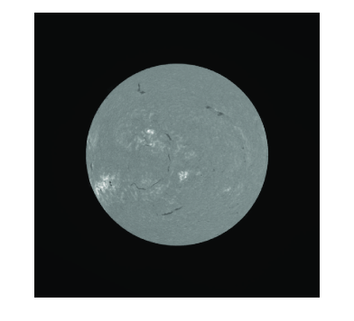
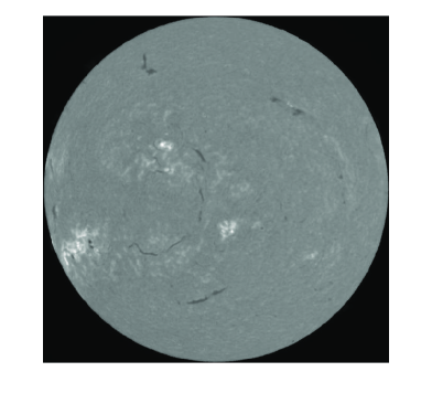
(a)                                  (b)

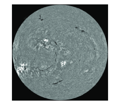
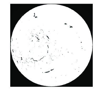
(c)                                  (d)

Figure 1.: An example of the H$\alpha$ image at 18:08:52 UT, 20 April 2001, obtained by Mauna Loa Solar Observatory (MLSO). (a) The original corrected image downloaded from the MLSO web site. (b) The sub-image extracted from panel (a). (c) The enhanced image after the top-hat transformation. (d) The image after a threshold filtering. mlso˙pre

2.5 Threshold Filter

On the solar disk in H$\alpha$, besides the dark features such as filaments and sunspots, there are some other bright features such as plages and flares. Many authors used local threshold method to filter out these non-interesting features. Actually, after limb-darkening removal and top-hat filtering,we can easily distinguish the filaments from these non-filament structures in the gray-scale images via the global threshold method.We tested several hundred images to find the appropriate global threshold value. For MLSO images, we found that the threshold value is about 95–100. The algorithm is simple: if the pixel’s value is greater than the threshold value, we assign it to be 255, which means white in the image. An example is shown in Figure mlso_pre(d).

3 Filament Detection

Detection

3.1 Canny Edge Detection

Segmentation of an image entails the division or separation of the image into regions of similar attributes [Pratt (2001)]. The most basic attribute for segmentation is the intensity level for a gray-scale image and color components for a color image. In addition, the image edge is also a useful attribute for segmenting.It is possible to segment an image into regions of common attribute by detecting the boundary of each region across which there is a significant change in intensity. We adopt the most powerful edge-detection method, i.e. the Canny method [Canny (1986)], to identify filaments. The Canny method differs from other edge-detection methods in that it uses two different thresholds: one for detecting strong edges and the other for weak edges. The weak edges are included in the output only if they are connected to strong edges. Compared to others, this method is therefore less fooled by noise, and is more likely to detect true weak edges [Lim (1990)]. The Canny method works in a multi-step process:

Step 1: Noise reduction. Because the Canny edge detector is susceptible to noise present in the image data, the image should be smoothed first. In our method, each image after preprocessing is smoothed by Gaussian convolution as follows,

$$\ilabel{edge1-equation}G(x,y)=\frac{1}{2\pi\sigma^{2}}{\rm e}^{-\frac{x^{2}+y^{2}}{2\sigma^{2}}}\,,$$ (2)

$$\ilabel{edge2-equation}f^{\prime}(x,y)=\sum_{x^{\prime}}\sum_{y^{\prime}}f(x,y)G(x-x^{\prime},y-y^{\prime})\,,$$ (3)

where $G(x,y)$ is the 2D Gaussian filter; $f(x,y)$ is the input image and $f^{\prime}(x,y)$ is the output image which is convolved with the 2D Gaussian filter; ($x,y$) is the position in the $x$–$y$ plane of the image. We choose $\sigma=1$ in our processing.

Step 2: Finding gradients. The edges usually can be found at those places where the gray-scale intensity drastically changes. It means that we can find them by checking the gradient at each pixel in the image. The first is to get the gradient in the $x$-direction $g_{x}(x,y)$ and $y$-direction $g_{y}(x,y)$, respectively, by applying the derivative of a Gaussian filter:

$$\ilabel{edge3-equation}g_{x}(x,y)=\sum_{x^{\prime}}\sum_{y^{\prime}}f(x,y)g_{1}(x-x^{\prime},y-y^{\prime})\,,$$ (4)

$$\ilabel{edge4-equation}g_{y}(x,y)=\sum_{x^{\prime}}\sum_{y^{\prime}}f(x,y)g_{2}(x-x^{\prime},y-y^{\prime})\,,$$ (5)

where

$$\ilabel{edge5-equation}g_{1}(x,y)=-\frac{1}{\pi\sigma^{2}}x{\rm e}^{-\frac{x^{2}+y^{2}}{2\sigma^{2}}}\,,$$ (6)

$$\ilabel{edge6-equation}g_{2}(x,y)=-\frac{1}{\pi\sigma^{2}}y{\rm e}^{-\frac{x^{2}+y^{2}}{2\sigma^{2}}}.$$ (7)

Then we use the following two equations to determine the gradient magnitude and the direction of the edge:

$$\ilabel{gradient-equation}g(x,y)=\sqrt{g_{x}(x,y)^{2}+g_{y}(x,y)^{2}}\,,$$ (8)

$$\ilabel{gradient-dir-equation}\theta(x,y)=\arctan\frac{g_{y}(x,y)}{g_{x}(x,y)}\,.$$ (9)

Step 3: Non-maximum suppression. For an image array, the edge direction angle is rounded to one of four angles representing vertical, horizontal and the two diagonals (i.e. 0, 45, 90, 135, 180, 225, 270, 315 and 360 degrees), corresponding to the use of an 8-connected neighbourhood. Then, for each pixel of the gradient image, we compare the edge gradient magnitude of the current pixel with the edge gradient magnitude of the pixel along the gradient direction. For example, if the gradient direction is to the northeast, the pixel should be compared with the pixels to the northeast and to the southwest. If the edge gradient magnitude of the current pixel is the largest one, we mark it as one part of the edge. If not, we suppress it, i.e. it is ignored.

Step 4: Edge tracing by hysteresis. After step 3, many of the remaining edge pixels would probably be the true edges of filaments, but some may be caused by noises. The Canny method uses thresholding with hysteresis to determine whether the edges obtained in step 3 are true or not. The algorithm adopts two thresholds, i.e. high and low thresholds: If the edge pixel’s gradient magnitude is higher than the high threshold, the pixel is marked as a strong pixel; if the edge pixel’s gradient magnitude is lower than the low threshold, the pixel will be suppressed; if it is between the two thresholds, the pixel will be marked as a weak one.

In order to find the thresholds, we use an automatic method: First, we should provide a probability of the pixels that are not the edge points and calculate the number of pixels that may not be the edge points in the entire image by the probability; Then we increase the gradient threshold until the total number of the pixels with the gradient smaller then the threshold is just greater than the probability value, then the current gradient threshold is chosen as the high threshold. The low threshold is about half of the high one. In our process the probability is chosen to be about 0.98, and the low threshold is 0.4 times the high threshold.

After tracing through the entire image we have strong and weak pixel arrays which can be treated as a set of edge curves. The weak edges are included if and only if they are connected to strong edges. We scan the entire binary image to find the pixels where strong and weak edges overlap each other and finally get the edge map. Then, the morphological thinning operation [Lam, Lee, and Suen (1992)] is applied to minimize the connected lines in order to get accurate and fine edges.

After applying the Canny edge-detection method, we get the edge of each filament, as shown in Figure mlso_detection(a).

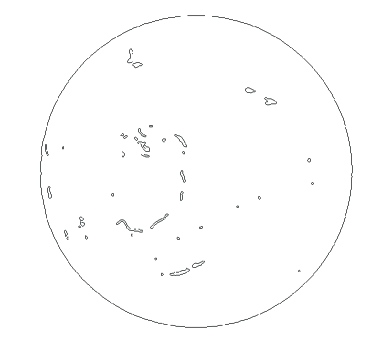
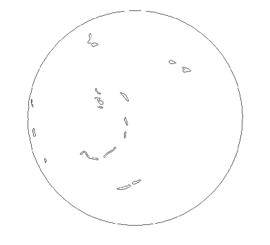
(a)                                  (b)

Figure 2.: Examples after filament detection processing. (a) After Canny edge detection, the filaments were segmented, the result shows the edge of each filament or fragment. (b) The image after sunspot removal. Compared with (a), small cycles (i.e. the edges of sunspots) were removed. In order to obtain clear results, the foreground and background colors are exchanged, i.e. the filament features become black and the background becomes white. The same is for Figure mlso_feature. mlso˙detection

3.2 Connected Component Process

After segmentation process, in the computer vision the image is still an array of pixels. We are not interested in each pixel but the special region (i.e. the filament) constituted by the pixels. These regions are called the connected components of the binary images, which are more complex and have a rich set of properties (i.e. shape, position, and area). We use a classical method [Haralick and Shapiro (1992)] to realize the connected component labeling. It means that the pixels in a connected component are given with the same identity label. After connected component labeling, the product we get is changed from pixels to regions that we are interested in. The input binary images are of 8-connectivity, and the algorithm consists of the following two steps:

In the first step, the algorithm goes through each pixel from left to right and from top to bottom, as indicated by the arrows shown in Figure connect_component_label(a). It checks the labels of four neighboring pixels that are north-east, north, north-west and west of the current pixel. For example, suppose the current pixel is $(i,j)$ as shown in Figure connect_component_label(a), the code checks the labels of four pixels that are $(i-1,j+1)$, $(i-1,j)$, $(i-1,j-1)$, and $(i,j-1)$ :

i) If all four neighbors are not assigned, a new label is assigned to the current pixel. An example is shown in Figure connect_component_label(b): Supposing that the value of the current pixel is 1 and the values of the four neighbors are 0 (0 means this pixel is a background pixel, and 1 means the pixel is the foreground), it means a new filament is encountered. If the previous label is “2”, we assign label “3” to the new filament.

ii) If one of the four neighbors has been labeled before, we assign the neighbor’s label to the current pixel. An example is shown in Figure connect_component_label(c): One of the four neighbors has been labeled, i.e. the north neighbor has been labeled “3”, so we assign the same label to the current pixel.

iii) If more than one of the neighbors have been labeled before, we assign the smaller label to it. An example is shown in Figure connect_component_label(d): Two neighbors have been labeled, i.e. the north-east and west neighbors. The label of north-east neighbor is “3”, which is smaller than the west neighbor’s, so we use ”3” to assign the current pixel.

After completing the scanning, the equivalent label pairs are sorted into equivalence classes and a unique label is assigned to each class.

In the second step, the above algorithm goes through again, during which each label is replaced by the label assigned to its equivalence class. After completing the scanning, a unique label is assigned to each equivalence class. In other words, we have assigned each filament a unique label.

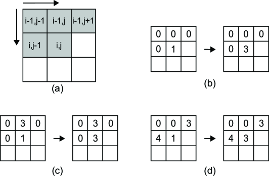
Figure 3.: Scanning sequence (panel a) and three examples for the connected components label method (panels b, c, and d). connect˙component˙label

3.3 Sunspot Filter

Actually, it is not easy to distinguish between sunspots and filaments by gray-scale levels. The labeled “filaments” so far may include some sunspots. Thus, we have to separate real filaments from sunspots by use of geometric structures: the size and the long-to-short-axis ratio of the filament.A candidate with the size (e.g. the perimeter) larger than the threshold is considered to be a filament. In the case that the size of the labeled object is smaller than the size threshold, only if the ratio of the long axis to short axis is larger than a given value, the candidate is treated as a small filament; otherwise it would be removed. We have got the edge of each filament whose length can be treated as the filament perimeter. We set the perimeter threshold to be 25 pixels, and the long-to-short-axis ratio threshold being 2 in our procedure. An example is shown in Figure mlso_detection(b). The filament label should be updated after removing the sunspots. Then each filament is labeled with a unique number. An example is shown later in Figure mlso_update(a). This method is used to filter out sunspots. With the same method, we can filter out other features. In other words, we can adopt the method to automatically detect sunspots, which will be implemented in our future work.

4 Filament Feature Recognition

Feature

4.1 Perimeter

As mentioned above, we have the filament edge, which can be easily used to derive the filament perimeter after the connected component process. It is done by the integration of the distance connecting neighboring pixels along the edge of each filament.

4.2 Position

We choose the geometric center of each filament, i.e. the centroid, as the location of the filament. First, we find the centroid of a filament ($x_{c},y_{c}$), i.e. we calculate the average of the abscissa and the ordinate of all the filament pixels. Since filaments follow the solar rotation and the rotation axis wobbles with time, the position of a certain filament has an elliptic orbit in the plane of the sky. In order to get the longitude and the latitude of the filament in the heliographic coordinates, we use the Solar SoftWare routine “xy2lonlat.pro”.

It is noted that the center of the solar disk we used here is not that provided in the header of the “FITS” file. After the Canny edge detection, besides the locations of the filaments, we also got the boundary of the solar disk, and it is the biggest connected component after the connected component processing. We fit the circle and calculate the geometric center of the fitted circle, which is the exact center of the solar disk.

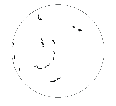
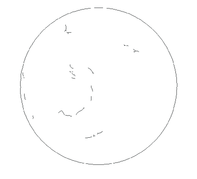
(a)                                  (b)

Figure 4.: Examples of filament feature recognition. (a) The image after morphological reconstruction processing, the edge curve is full filled with white pixels, from which we get the filament area. (b) The filament spines after morphological skeletonization and barbs removal processing. mlso˙feature

4.3 Area

In our process, the area of a filament is the integration of the pixel area divided by the cosine of the heliocentric angle, where the integration is taken in the area enclosed by the edge curve. We use the foreground color (white) to fill the edge curve so that the pixels inside the curve become white, then the white pixels constitute the filament area. The algorithm is based on morphological reconstruction [Soille (1999)]. The edge curve with holes is filled with white pixels. The hole is a set of background pixels (i.e. black pixels) surrounded by foreground pixels (white pixels). An example is given in Figure mlso_feature(a) and an extracted filament example is shown in Figure feature_example(c).

4.4 Spine

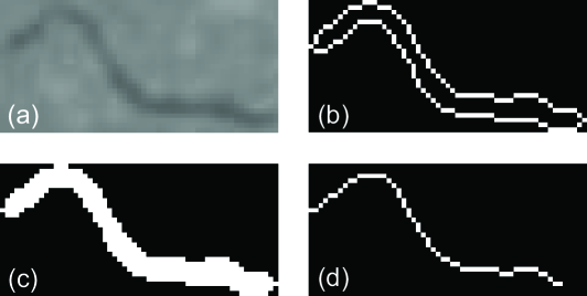
Figure 5.: An example of a filament feature recognition. (a) A filament extracted from the original image (i.e. Figure mlso_pre(a)). (b) The filament edge (i.e. the perimeter). (c) The filament edge was filled with white pixels, from which we got the filament area. (d) The filament skeleton (i.e. spines). feature˙example

The morphological skeletonization method is adopted to get the filament spine, which is a stick-like skeleton, spatially placed along the medial region of the filament. The skeleton is a unit-wide set that contains only the pixels that can be removed without changing its topology [Kong and Rosenfeld (1996)]. Iterations of the morphological-thinning operation are employed for the skeleton method [Haralick and Shapiro (1992)]. Assuming that the input binary image is $I$ (i.e. a matrix only has values of 0 and 1), the details of the method are described below:

First, the thinning processing of $I$ by structuring-element pair $(J,K)$ is defined as

$$I\oslash(J,K)=I-I\otimes(J,K)\,,$$ (10)

where $\oslash$ is the morphological thinning operator, $J$ and $K$ must satisfy $J\cap K=\emptyset$, where the symbol $\emptyset$ represents the empty set. $I\otimes(J,K)$, i.e. the hit-and-miss transformation of set $I$ by $(J,K)$, is defined by

$$I\otimes(J,K)=(I\ominus J)\cap(I^{c}\ominus K)\,,$$ (11)

where $\otimes$ is the hit-and-miss transformation operator, $\cap$ the intersection operator, $I^{c}$ the complement of $I$ and the symbol $\ominus$ denotes the morphological erosion operator.

Then, using the sequence of eight structuring-element pairs as shown in Figure jk_array to iteratively process the thinning operation:

$$I_{N+1}=(\ldots\{[I_{N}\oslash(J_{1},K_{1})]\oslash(J_{2},K_{2})\}\oslash\ldots\oslash(J_{8},K_{8})).$$ (12)

We let $I_{0}=I$, which is firstly thinned by the structure-element pair $(J_{1},K_{1})$, and then by $(J_{2},K_{2})$, …, $(J_{8},K_{8})$, the thinned result is defined as $I_{1}$. Such a process is repeated in order to get $I_{2}$, $I_{3}$, …, $I_{N}$.

Finally, the thinning process repeats until $I_{N}=I_{N+1}$, i.e. the filament skeleton is the final structure that can not be thinned any more. Actually, some of the resulting filament skeletons still contain small barbs. We use the morphological hit-and-miss transformation to find the endpoints that constitute the barbs, and then remove the barbs. This process may iterate several times because some of these points may not be removed in one go. In our process it is iterated four times. The filament spines on the whole Sun are shown in Figure mlso_feature(b) and an extracted filament example is shown in Figure feature_example(c).

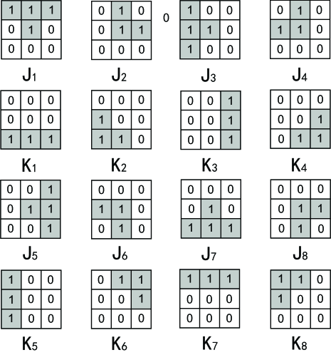
Figure 6.: Structuring-element pair $(J_{i},K_{i})$ used to determine the filament skeleton. $J_{i}$ and $K_{i}$ must satisfy $J_{i}\cap K_{i}=\emptyset$. jk˙array

4.5 Tilt Angle

The tilt angle is defined as the fitted filament spine orientation with respect to the solar Equator. After we get the spine, we use a linear polynomial to fit it, by which we calculate the slope $A$. The tilt angle is $\arctan(A)$.

4.6 Feature Update

A filament may consist of several fragments. Thus, the filaments we obtained after the previous processing may not be the real individual filaments, with some being fragments of one filament. We adopt a “distance criterion” in order to find the fragments belonging to a single filament. The method is the same as the “labelling criterion” filament tracking method used by Joshi2010, which is explained as follows: For a certain filament or filament fragment, we compare it with all other fragments. The fragments would be recognized to belong to a common filament if the two fragments lie within the distance threshold. The process is iterated until all fragments are checked. The filaments in the new image are compared with those in the previous image. The experiential distance threshold in our processing is taken to be 60 pixels for the MLSO data. After this process, the fragment labels will be updated; if several fragments belong to a common filament, the label should be unified, as shown in Figure mlso_update(b). For example, filament fragments number 11 and 15 in Figure mlso_update(a) are recognized as one filament, thus they are updated with the same label number 7. For the update of the area, perimeter, and the length of spine, we just calculate the sum of each fragment with the same label, while the position and the tilt angle must be reprocessed.

Another criterion for identifying a broken filament is to compare the tilt angle of the fragments, i.e. if the neighboring candidates have similar tilt angles, they could be considered as one big filament. This method works fine for the magnetic inversion lines that are not strongly curved, and will be incorporated in our future version.

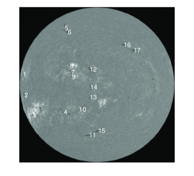
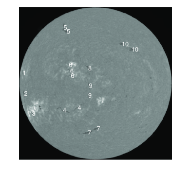
(a)                                  (b)

Figure 7.: An example of the detection results. (a) After filament detection, each filament or fragment is labeled with a unique number. It shows there are in total 17 filaments or fragments, and each of their centers is labeled with a unique number. (b) Each candidate filament that we obtained after the filament detection processing may not be a true one but a filament fragment. After the feature update processing, the fragments belonging to a single filament are labeled with the same number. For example, filament fragments numbers 11 and 15 in (a) were recognized as one filament, thus they are updated with the same label number 7 in panel (b). mlso˙update

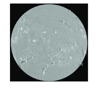
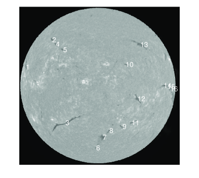
(a)                                  (b)

(c)                                  (d)

Figure 8.: An example of filament tracing method between two images at 18:41:38 UT, 17 February 2001 and at 18:41:40 UT, 18 February 2001 respectively obtained by MLSO. (a) The detected result of the earlier image, each filament is labeled with a unique number. (b)the detected filament fragments are shown individually; (c) the updated filaments where fragments are labelled to be one filament. (d) Final result, where the labels of the traced filaments are updated. mlso˙trace

5 Filament tracing

Tracing

Tracing the evolution of the filament is important for understanding the physical nature and the solar cyclic variation of the filaments. In this section we present a tracing method. Here we use the filament label, position and area as the input parameters, which have been obtained in Section Feature, to trace the daily evolution of the filaments.

We define two input images as $I_{\rm old}$ (i.e. the image observed at the old time) and $I_{\rm new}$ (i.e. the image at the new time). The main steps of the tracing method are as follows:

i) We obtain the observation time of the two images $I_{\rm old}$ and $I_{\rm new}$, then calculate the time interval $T_{\rm interval}$;

ii) Using the latitude from the position features of each filament in $I_{\rm old}$ (or $I_{\rm new}$) in order to calculate the rotation velocity at this latitude $\omega_{\rm old}$ (or $\omega_{\rm new}$), then calculate the possible longitude $PLO_{\rm old}$ (or $PLO_{\rm new}$) with the time interval $T_{\rm interval}$. Here the $PLO_{\rm new}$ is calculated by assuming that the Sun rotates backward;

$$PLO_{\rm old(\textit{i})}=CLO_{\rm old(\textit{i})}+\omega_{\rm old(\textit{i})}\cdot T_{\rm interval}\,(i=1,2,\ldots,n)\,,$$ (13)

$$PLO_{\rm new(\textit{j})}=CLO_{\rm new(\textit{j})}-\omega_{\rm new(\textit{j})}\cdot T_{\rm interval}\,(j=1,2,\ldots,n)\,,$$ (14)

where $CLO_{\rm old(i)}$ (or $CLO_{\rm new(j)}$) is the current longitude of $i$-th (or $j$-th) filament in $I_{\rm old}$ (or $I_{\rm new}$). Here, we adopt the solar rotation angular velocity formula [Balthasar, Vazquez, and Wöehl (1986)] to determine $\omega_{\rm old(i)}$ and $\omega_{\rm new(j)}$:

$$\omega(\theta)=(14.551\pm 0.006)-(2.87\pm 0.06)\sin^{2}\theta\,,$$ (15)

where $\omega$ is the angular velocity (degrees per day) and $\theta$ the latitude;

iii) We obtain the possible position [$PP_{\rm old}:(PLA_{\rm old},PLO_{\rm old})$] of the filament after $T_{\rm interval}$ via the differential rotation formula, then calculate the distance $D_{\rm old\rightarrow new}$ between $PP_{\rm old}$ and real current position [$CP_{\rm new}:(CLA_{\rm new},CLO_{\rm new})$] of the filament in $I_{\rm new}$. Because the drift velocity of the filament is much smaller than the solar rotation velocity, we assume the filament latitude does not change in $I_{\rm old}$ (i.e. $PLA_{\rm old}=CLA_{\rm old}$, $PLA_{\rm old}$ is the possible latitude and $CLA_{\rm old}$ is the current latitude in $I_{\rm old}$). The distance $D_{\rm old\rightarrow new}$ between $PP_{\rm old}$ and $CP_{\rm new}$ is:

$$D_{\rm old{\rightarrow}new}=\sqrt{(PLA_{\rm old}-CLA_{\rm new})^{2}+(PLO_{\rm old}-CLO_{\rm new})^{2}}\,.$$ (16)

iv) We assume that the Sun rotate backward, then obtain the possible position of the filament [$PP_{\rm new}:(PLA_{\rm new},PLO_{\rm new})$] after $T_{\rm interval}$. A processing which is similar to 3) is processed, the distance $D_{\rm new{\rightarrow}old}$ between $PP_{\rm new}$ and $CP_{\rm old}$ is:

$$D_{\rm new{\rightarrow}old}=\sqrt{(PLA_{\rm new}-CLA_{\rm old})^{2}+(PLO_{\rm new}-CLO_{\rm old})^{2}}\,.$$ (17)

v) For each filament in $I_{\rm new}$, we check all of the filaments in $I_{\rm old}$. Only if one meets the following three conditions, the filament in $I_{\rm old}$ would be considered to be the same filament and marked with the same label as in $I_{\rm new}$:

Condition 1: $D_{\rm old{\rightarrow}new}\leq{ED_{1}}\cdot T_{\rm interval}$;

Condition 2: $D_{\rm new{\rightarrow}old}\leq{ED_{2}}\cdot T_{\rm interval}$;

Condition 3: $Area_{\rm old(\textit{current})}/Area_{\rm new(\textit{j})}\geq{ratio},(j=1,2,\ldots,n),$

where $ED_{1}\cdot T_{\rm interval}$ and $ED_{2}\cdot T_{\rm interval}$ are the distance threshold. In our program we take $ED_{1}=ED_{2}=100$ pixels day^-1. $Area_{\rm old(\textit{current})}$ and $Area_{\rm new(\textit{j})}$ are the filament area at the old and new times, respectively. Condition 3 gives the maximum proportion of the deformation, i.e. less than the specified $ratio$ of the size of the previous filament. Here we set $ratio=50\%$ . If the three conditions are not satisfied, the filament at the new time would be identified as a new filament and given a new label. This step continues until all filaments in $I_{\rm new}$ are treated. Finally, the filament labels in $I_{\rm new}$ are updated. Figure mlso_trace gives an example of our tracing method, where panel (a) shows the detected result of the earlier image with each filament labeled a unique number, panel (b) depicts the filament fragments after detection, penel (c) shows the updated filaments where several fragments merged into one filament, and panel (d) shows the tracing result based on the earlier image in panel (a). For example, the filament 2 in the earlier image (panel a) is split into three fragments (labeled 2, 4, and 5 in the later image (panel b). After using the tracing method, they were labeled the same number in the earlier image (panel a). Filament 13 in the later image (panel d) was not detected in the earlier image (panel a), so it was given a new number.

6 Performance

Performance

Our code was developed by using $\rm MATLAB^{\tiny\circledR}$ Desktop Tools and Development Environment on a desktop computer (CPU: $\rm Intel^{\tiny\circledR}\ \rm Core^{\tiny TM}$ Duo 3.00 GHz). After processing of each image file, the result (such as the label, the position, the area, and other features) are written to a text file. The average processing speed is 1 second for the filament detection in a single image and 3.5 seconds for the filament detection and tracing in two images. We randomly selected 100 images from the MLSO H$\alpha$ archive for testing, and compared the automated result with the manual ones. For filaments and filament fragments, the two methods are overlapping by $85\pm 2\%$ and $88\pm 4\%$, respectively. The error includes two types of false recognition: One is that there is a manually recognized filament, but the automated method cannot detect it. The other is that the automated method detects a filament, but it does not appear on the real solar disk. It is noted that the latter is rarely seen in our method. If a filament splits into several small fragments, and the criterion of the ratio of the long to short axes is not satisfied (i.e. being recognized as a sunspot), our method may miss these fragments. The accuracy of the filament fragment number is a little higher than that of the filament, which is due to the prescribed “distance criterion”. Sometimes several filaments or filament fragments in one active region are so close to each other and within the “distance criterion”, they are recognized as one filament. This kind of false recognition does appear in our filament fragment detection and we have to improve the filament fragments merging method in the future. For other features such as position, perimeter, area, and spine, there are no standard criteria to test the accuracy of the results processed by our codes. However, we defined two indices in order to test the performance of our method, i.e. the “edge closed rate” and the “area fully filled rate”. The “edge closed rate” is defined as the number of detected filaments with edge curve closed as a percentage of the total number of detected filaments among the 100 test images. We found that the rate is 91%. This rate mainly depends on the selection of the threshold in the threshold filter processing and the two thresholds in the Canny edge-detection method. If the filament edge curve is not closed, it leads to low detection accuracy and affects the subsequent processing. The “area fully filled rate” is defined as the number of the detected filaments with edge curve fully filled with foreground pixels as a percentage of the total number of detected filaments among the 100 test images, and the rate is 75%. After the edge detection is finished, if the edge curve is not closed, the morphological object filling method could not fully fill in the area enclosed by the edge curve. This leads to the decrease in “area fully filled rate” and the detection accuracy rate. The filament spine is also affected by the area problem, i.e. if the area is not fully filled, our method may get a wrong topology of the filament after the morphological skeletonization processing. Furthermore, if the barbs are located near the end of the filament spine or the filament size is relatively small, the recognized spine may be shorter than the real length after the morphological barb removal processing. The shorter the time interval is, the higher the tracing accuracy is. Here, we set the default time interval to be about one day, the accuracy of the tracing method is about 80%. In addition, we also test images from Big Bear Solar Observatory (BBSO) H$\alpha$ archive (ftp://ftp.bbso.njit.edu/pub/archive) to validate the versatility of our method. The results are similar and satisfactory.

7 Statistical Results of the Filament Latitude

Results

We use our automated method to analyze 3470 images obtained by MLSO from January 1998 to December 2009. In this section, we present the statistical results of the evolution of the filament latitudinal distribution because of its relatively high accuracy. Furthermore, from a statistical point of view, such results can be significant in understanding the cyclic migration of solar filaments.

7.1 Butterfly Diagrams

For the period from January 1998 to December 2009, we process one image per day and have detected 13,832 filaments. The temporal evolution of the latitudinal distribution of these filaments is depicted as the scatter plot in Figure BFD_f (each dot represents a single observation), where we can clearly see a butterfly diagram, similar to sunspots. Because of the lack of observations in some periods, there are several white vertical gaps in the butterfly diagram. From the diagram we can see the distribution and the migration of the filaments. This butterfly diagram indicates that the formation of the filaments mainly migrates towards the equator from the beginning to the end of the Solar Cycle 23.

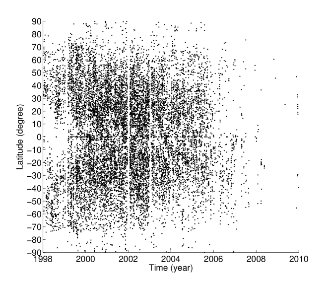
Figure 9.: Butterfly diagram of filaments from January 1998 to December 2009 in the Solar Cycle 23. Each dot represents a single observation.BFD˙f

7.2 Drifting Velocity

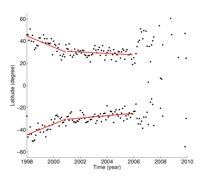
Figure 10.: Temporal evolution of the monthly mean latitudinal distribution of filaments from January 1998 to December 2009. Linear fittings are shown by solid-red lines. mm˙total

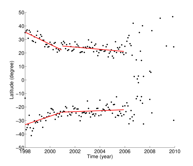
Figure 11.: Temporal evolution of the monthly mean latitudinal distribution of filaments with a latitude lower than $50^{\circ}$ from January 1998 to December 2009. Linear fittings are shown by solid-red lines. mm˙0-50

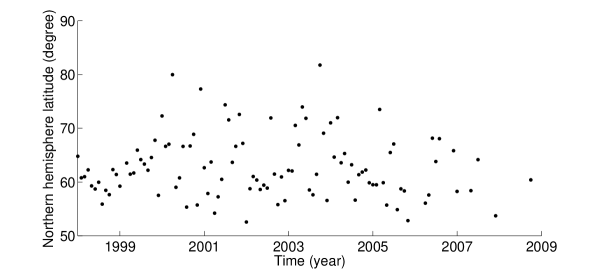
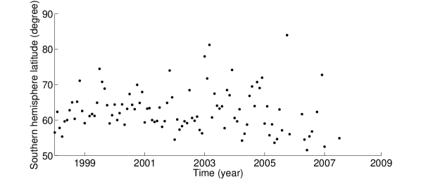
Figure 12.: Temporal evolution of the monthly mean latitudinal distribution of the filaments with latitude higher than $50^{\circ}$ from January 1998 to December 2009. The upper panel is for the northern hemisphere and the bottom panel is for the southern hemisphere.mm˙50-90

From the butterfly diagram we only get qualitative results, as mentioned by 2010Li. In order to make a quantitative analysis, we adopt the monthly mean latitude of the filaments in the northern and southern hemispheres, respectively. The calculated results are plotted in Figure mm_total. It can be seen that the monthly mean latitudinal distribution of the filaments has three drift trends: from 1998 to the solar maximum (2001) the drift velocity is very fast. After the solar maximum it becomes relatively slow. After 2006, the drift velocity becomes divergent. A linear fitting is used to the data points in different periods, resulting in an average drift velocity being 0.0138 degree day^-1, or 1.86 m s^-1, during 1998–2001, and 0.0017 degree day^-1 or 0.23 m s^-1 during 2002–2006 in the northern hemisphere. It is 0.0134 degree day^-1, or 1.80 m s^-1 during 1998–2001 and 0.0029 degree day^-1, or 0.39 m s^-1 during 2002–2006 in the southern hemisphere. Here, we did not fit the monthly mean filament distribution after 2006, because it becomes divergent near the solar minimum.

Since the normal solar activity is usually applied to the events with latitudes lower than $50^{\circ}$ [Sakurai (1998), Li et al. (2008)], we analyze the filaments with latitudes lower than $50^{\circ}$. The calculated result is plotted in Figure mm_0-50. It can be seen that the monthly mean latitudinal distribution of these filaments again has three drift trends: From 1998 to the solar maximum (2001) the drift velocity is fast, i.e. 0.0123 degree day^-1 or 1.66 m s^-1 in the northern hemisphere and 0.086 degree day^-1 or 1.16 m s^-1 in the southern hemisphere. After the solar maximum the drift velocity becomes relatively slow, i.e. 0.0022 degree day^-1 or 0.29 m s^-1 in the northern hemisphere and 0.0010 degree day^-1 or 0.13 m s^-1 in the southern hemisphere, respectively. After 2006 it becomes divergent. These results are similar to those of the entire latitudinal distribution. The reason is easy to understand: among the 13,832 filaments we detected, only 1,130 filaments have latitudes higher than $50^{\circ}$. In other words, the detected filaments are mainly distributed in latitudes lower than $50^{\circ}$. There is no obvious difference between the northern and the southern hemispheres. These results are similar to the statistical results of 2010Li. Similarly, we plot the monthly mean latitude of the filaments with latitudes higher than $50^{\circ}$ in Figure mm_50-90. However, no clear trend is discernible.

  

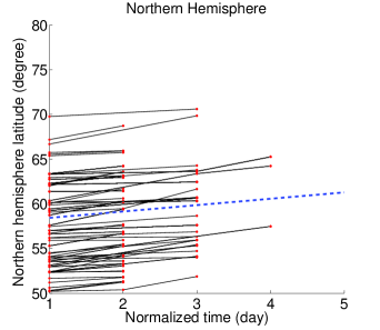
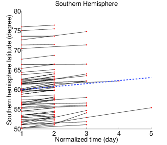
Figure 13.: Traced filament latitude variation versus normalized time. Here the normalized time means that we put the dates of the first detection of the filaments as the start time.The left and right panels are for the northern and southern hemisphere, respectively. The solid-black line represents the temporal and spatial variation of the traced filament latitudes, and the red dot indicates the filament where and when it was detected and traced. The dash-blue line is the linear fitted average of all traced filament temporal and spatial variations. normalized

  

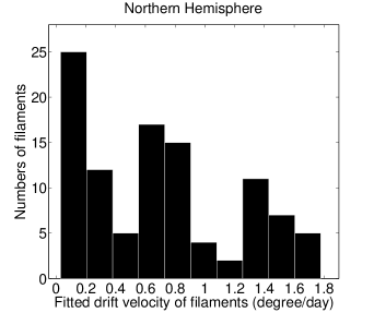
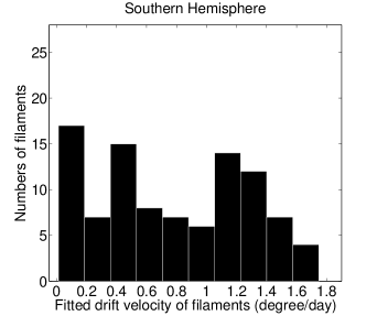
Figure 14.: Histograms of the drift velocity distribution of the filament whose latitudes are higher than $50^{\circ}$. The left panel is for the northern hemisphere with 103 filaments in total and the right panel for the southern hemisphere with 97 filaments in total. hist

In order to find the migration of the individual filaments above $50^{\circ}$, we employ our tracing method and set three additional conditions for tracing:

Condition 1: The filament positions are higher than $50^{\circ}$ at the first detection;

Condition 2: The time interval is less than two days. In other words, in three consecutive days, observations are available in at least two days. The purpose of this condition is to improve the accuracy.

Condition 3: The total time lapse should be less than ten days, because one specific filament observation can be clearly visible in less than a half-period of the solar rotation. If the time lapse is greater, the accuracy of the tracing method is lower.

We plot the tracing results of the latitude versus normalized time in Figure normalized. Here the normalized time means that we put the dates of the first detection of the filaments as the start time. The drift velocity distribution histograms in the northern hemisphere and the southern hemisphere are shown in Figure hist. In the northern hemisphere, there are 103 filaments (which occupy 57% of all filaments satisfying the conditions and being traced with the latitude higher than $50^{\circ}$), which migrate towards the polar region. The average drift velocity is 0.7126 degree day^-1 (96.2 m s^-1). In the southern hemisphere, there are 97 filaments (which occupy 61% of all filaments satisfying the conditions and being traced with latitude higher than $50^{\circ}$), which migrate towards the polar region. The average drift velocity is 0.7771 degree day^-1 (104.9 m s^-1). From Figure hist, we found that the drift velocities of the filaments with latitudes higher than $50^{\circ}$ are divergent, while most of these filaments migrate towards the polar region with relatively high velocities. Such a result is similar to that of 1982Topka. However, they found that the poleward drift velocity is about 10 m s^-1, which is much slower than ours.

8 Conclusions

Conclusion We have developed a method to automatically detect and trace solar filaments from H$\alpha$ full-disk images. The program consists of three parts: First, a preprocessing module is applied to correct the original images. Top-hat enhancement enables us to clearly distinguish the filaments from non-filament features. Second, we introduce the Canny edge-detection method to segment and detect filaments. This method gives us a precise filament edge. Third, our program routines recognize filament features through the morphological operators. We randomly selected 100 images from MLSO observations to test our method, which is demonstrated to be robust and efficient. For the filament detection, the similarity between the machine recognition and human vision is $85\pm 2\%$. The solar rotation, the filament position, and the deformation of the filament have been considered in order to trace the filament evolution. The accuracy of the tracing method is about 80% when the time interval is about one day. In addition, our program can process images not only in different file formats, but also from different observatories.

We used our method to automatically process and analyze 3470 images obtained by MLSO from January 1998 to December 2009 . A butterfly diagram of filaments is obtained, where we can clearly see that filaments move mainly towards the equator in both hemispheres. In order to obtain more quantitative results, we calculated the monthly mean latitudes of the filaments whose latitudes are within $0^{\circ}-50^{\circ}$ or higher than $50^{\circ}$ in both northern and southern hemispheres, respectively. Furthermore, we use our tracing method to trace the evolution of the individual filaments with a latitude higher than $50^{\circ}$. Our main conclusions are listed as follows:

$\bullet$ The latitudinal migration of solar filaments have three trends in the Solar Cycle 23: from 1998 to 2001 (the solar maximum) the drift velocity is fast. From the solar maximum to the year 2006 the drift velocity becomes relatively slow. After 2006, i.e. near solar minimum, the migration becomes divergent.

$\bullet$ About 60% filaments with latitudes higher than $50^{\circ}$ migrate towards the polar region with relatively high velocities in both northern and southern hemispheres.

$\bullet$ The difference of the latitude migration of the filaments between the northern and southern hemispheres is not obvious in the Solar Cycle 23.

We will improve our method to be more reliable and efficient, and apply it to the observational data from our Optical & Near Infrared Solar Eruption Tracer (ONSET) in Nanjing University [Fang et al. (2012)].

Acknowledgements

The authors thank the Mauna Loa Solar Observatory team for making the data available and Sun J. Q. for his help in identifying filaments. We also thank the referee very much for the constructive suggestions which greatly improved the paper in various ways. This work is supported by the National Natural Science Foundation of China (NSFC) under the grants 10221001, 10878002, 10403003, 10620150099, 10610099, 10933003, 11025314, and 10673004, as well as the grant from the 973 project 2011CB811402.

References

- Balthasar, Vazquez, and Wöehl (1986) Balthasar, H., Vazquez, M., Wöehl, H.: 1986, Astron and Astrophys 155, 87.
- Bernasconi, Rust, and Hakim (2005) Bernasconi, P.N., Rust, D.M., Hakim, D.: 2005, Solar Phys 228, 97. doi:10.1007/s11207-005-2766-y.
- Canny (1986) Canny, J.: 1986, Pattern Analysis and Machine Intelligence, IEEE Trans PAMI-8(6), 679. doi:10.1109/TPAMI.1986.4767851.
- Chen (2008) Chen, P.F.: 2008, Journal of Astrophysics and Astronomy 29, 179. doi:10.1007/s12036-008-0023-0.
- Chen (2011) Chen, P.F.: 2011, Liv Rev in Solar Phys 8, 1.
- Cox (2000) Cox, A.N.: 2000, Allen’s astrophysical quantities, 355.
- Fang et al. (2012) Fang, C., Chen, P.F., Ding, M.D., Dai, Y., Li, Z.: 2012, In: EAS Publications Series, EAS Publications Series 55, 349. doi:10.1051/eas/1255048.
- Fuller, Aboudarham, and Bentley (2005) Fuller, N., Aboudarham, J., Bentley, R.D.: 2005, Solar Phys 227, 61. doi:10.1007/s11207-005-8364-1.
- Gao, Wang, and Zhou (2002) Gao, J., Wang, H., Zhou, M.: 2002, Solar Phys 205, 93.
- Gilbert et al. (2000) Gilbert, H.R., Holzer, T.E., Burkepile, J.T., Hundhausen, A.J.: 2000, Astrophys J 537, 503. doi:10.1086/309030.
- Gopalswamy et al. (2003) Gopalswamy, N., Shimojo, M., Lu, W., Yashiro, S., Shibasaki, K., Howard, R.A.: 2003, Astrophys J 586, 562. doi:10.1086/367614.
- Haralick and Shapiro (1992) Haralick, R.M., Shapiro, L.G.: 1992, Computer and robot vision, 1st edn. Addison-Wesley Longman, Boston. ISBN 0201569434.
- Jing et al. (2004) Jing, J., Yurchyshyn, V.B., Yang, G., Xu, Y., Wang, H.: 2004, Astrophys J 614, 1054. doi:10.1086/423781.
- Joshi, Srivastava, and Mathew (2010) Joshi, A.D., Srivastava, N., Mathew, S.K.: 2010, Solar Phys 262, 425. doi:10.1007/s11207-010-9528-1.
- Kong and Rosenfeld (1996) Kong, T.Y., Rosenfeld, A.: 1996, Topological algorithms for digital image processing, Elsevier, Netherlands, 300.
- Labrosse, Dalla, and Marshall (2010) Labrosse, N., Dalla, S., Marshall, S.: 2010, Solar Phys 262, 449. doi:10.1007/s11207-009-9492-9.
- Labrosse et al. (2010) Labrosse, N., Heinzel, P., Vial, J.-C., Kucera, T., Parenti, S., Gunár, S., Schmieder, B., Kilper, G.: 2010, Space Science Rev 151, 243. doi:10.1007/s11214-010-9630-6.
- Lam, Lee, and Suen (1992) Lam, L., Lee, S.W., Suen, C.Y.: 1992, IEEE Trans Pattern Analysis Machine Intelligence 14(9), 869.
- Li (2010) Li, K.J.: 2010, Mon Not Roy Astron Soc 405, 1040. doi:10.1111/j.1365-2966.2010.16508.x.
- Li et al. (2008) Li, K.J., Li, Q.X., Gao, P.X., Shi, X.J.: 2008, J Geophys Res (Space Physics) 113, 11108. doi:10.1029/2007JA012846.
- Lim (1990) Lim, J.S.: 1990, Two-dimensional signal and image processing, 478.
- Martens et al. (2012) Martens, P.C.H., Attrill, G.D.R., Davey, A.R., Engell, A., Farid, S., Grigis, P.C., Kasper, J., Korreck, K., Saar, S.H., Savcheva, A., Su, Y., Testa, P., Wills-Davey, M., Bernasconi, P.N., Raouafi, N.-E., Delouille, V.A., Hochedez, J.F., Cirtain, J.W., Deforest, C.E., Angryk, R.A., de Moortel, I., Wiegelmann, T., Georgoulis, M.K., McAteer, R.T.J., Timmons, R.P.: 2012, Solar Phys 275, 79. doi:10.1007/s11207-010-9697-y.
- Martin (1998) Martin, S.F.: 1998, Solar Phys 182, 107. doi:10.1023/A:1005026814076.
- McIntosh (1972) McIntosh, P.S.: 1972, Rev Geophys Space Phys 10, 837.
- Minarovjech, Rybansky, and Rusin (1998) Minarovjech, M., Rybansky, M., Rusin, V.: 1998, Solar Phys 177, 357.
- Mouradian and Soru-Escaut (1994) Mouradian, Z., Soru-Escaut, I.: 1994, Astron and Astrophys 290, 279.
- Pratt (2001) Pratt, W.K.: 2001, Digital Image Processing, 3rd edn. John Wiley & Sons, Hoboken. ISBN 0471221325.
- Qu et al. (2005) Qu, M., Shih, F.Y., Jing, J., Wang, H.: 2005, Solar Phys 228, 119. doi:10.1007/s11207-005-5780-1.
- Rusin, Rybansky, and Minarovjech (1998) Rusin, V., Rybansky, M., Minarovjech, M.: 1998, In: Balasubramaniam K. S., Harvey J., & Rabin D. (ed.) Synoptic Solar Physics, CS- 140, 353.
- Sakurai (1998) Sakurai, T.: 1998, In: Balasubramaniam K. S., Harvey J., & Rabin D. (ed.) Synoptic Solar Physics, CS- 140, 483.
- Shih and Kowalski (2003) Shih, F.Y., Kowalski, A.J.: 2003, Solar Phys 218, 99. doi:10.1023/B:SOLA.0000013052.34180.58.
- Soille (1999) Soille, P.: 1999, Morphological image analysis: Principles and applications 11, Springer, Secaucus, 173.
- Tandberg-Hanssen (1995) Tandberg-Hanssen, E. (ed.): 1995, The nature of solar prominences, Astrophys Space Science Lib 199, Dordrecht.
- Topka et al. (1982) Topka, K., Moore, R., Labonte, B.J., Howard, R.: 1982, Solar Phys 79, 231. doi:10.1007/BF00146242.
- Wang et al. (2010) Wang, Y., Cao, H., Chen, J., Zhang, T., Yu, S., Zheng, H., Shen, C., Zhang, J., Wang, S.: 2010, Astrophys J 717, 973. doi:10.1088/0004-637X/717/2/973.
- Yuan et al. (2011) Yuan, Y., Shih, F.Y., Jing, J., Wang, H., Chae, J.: 2011, Solar Phys 272, 101. doi:10.1007/s11207-011-9798-2.
- Zhang, Cheng, and Ding (2012) Zhang, J., Cheng, X., Ding, M.-D.: 2012, Nature Communications 3. doi:10.1038/ncomms1753.