Fault Tolerant Quantum Random Number Generator Certified by Majorana Fermions

Abstract

Braiding of Majorana fermions gives accurate topological quantum operations that are intrinsically robust to noise and imperfection, providing a natural method to realize fault-tolerant quantum information processing. Unfortunately, it is known that braiding of Majorana fermions is not sufficient for implementation of universal quantum computation. Here we show that topological manipulation of Majorana fermions provides the full set of operations required to generate random numbers by way of quantum mechanics and to certify its genuine randomness through violation of a multipartite Bell inequality. The result opens a new perspective to apply Majorana fermions for robust generation of certified random numbers, which has important applications in cryptography and other related areas.

The complex-valued solutions to the Dirac equation predict that every elementary particle should have a complex conjugate counterpart, namely an antiparticle. For example, an electron has a positron as its antiparticle. However, in $1937$ Ettore Majorana 1937Majorana showed that the complex Dirac equation can be modified to permit real wave-functions, leading to the possible existence of the so called “Majorana fermions” which are their own antiparticles 2009Wilczek . In condensed matter physics, Majorana fermions may appear as elementary qusi-particle excitations. To search for Majorana fermions, several proposals have been made in recent years, including $\nu=5/2$ fractional quantum Hall system 2010Stern ; 2008Nayak , topological insulator (TI)—superconductor (SC) interface 2008Fu , interacting quantum spins 2006Kitaev , chiral p-wave superconductors 2000Read , spin-orbit coupled semiconductor thin film 2010Sau or quantum nanowire 2010Lutchyn ; 2010Oreg in the proximity of an external s-wave superconductor. Based on these proposals, experimentalists have made great progress recently. For instance, Ref. 2012Wang reported an experimental observation of coexistence of the superconducting gap and the topological surface state in the $\mathtt{Bi}_{2}\mathtt{Se}_{3}$ thin film as a step towards realization of Majorana fermions. More recently, signature of Majorana fermions in hybrid superconductor-semiconductor nanowire device has been reported 2012Mourik , which has raised strong interest in the community.

Majorana fermions are exotic particles classified as non-abelian anyons with fractional statistics, and braiding between them gives nontrivial quantum operations that are topological in nature. These topological quantum operations are intrinsically robust to noise and experimental imperfection, so they provide a natural solution to realization of fault-tolerant quantum gates. Application of Majorana fermions in implementation of fault-tolerant quantum computation has raised great interest 2006Kitaev ; 2008Nayak . Unfortunately, braiding of Majorana fermions are not sufficient yet for realization of universal quantum computation 2008Nayak , and we need assistance from additional non-topological quantum gates which are prone to influence of noise.

In this Letter, we show that topological manipulation of Majorana fermions alone can be used to realize a quantum random number generator in a fault tolerant fashion and to certifies its genuine randomness through violation of the Mermin-Ardehali-Belinskii-Klyshko (MABK) inequality 1993Belinskii ; 1992Ardehali ; 1990Mermin . Random numbers have tremendous applications in science and engineering 2001Ackermann ; 1991Hultquist ; 2003Tu . However, generation of genuine random numbers is a challenging task 2010Pironio . Any classical device does not generate genuine randomness as it allows a deterministic description in principle. Quantum mechanics is intrinsically random, and one can explore this feature to generate random numbers 1956Isida ; 1990Svozil ; 1994Rarity ; 2000Jennewein . However, in real experiments, the intrinsic randomness of quantum mechanics is always mixed-up with an apparent randomness due to noise or imperfect control of the experiment 2010Pironio . The latter can be exploited by an adversary opponent and leads to security loopholes in various applications of randomness. Recently, a nice idea has been put forward to certify genuine randomness generated by a quantum device through test of violation of the Bell-CHSH (Clauser-Horn- Shimony-Holt 1969Clauser ) inequality 2007Colbeck ; 2010Pironio , and the idea has been demonstrated in a proof-of-principle experiment using remote entangled ions 2010Pironio . This implementation is not fault-tolerant yet as the remote entanglement is sensitive to noise and the quantum gates have limited precision which can all lead to security loopholes. We show here that all the operations for generation and certification of genuine randomness can be realized through topological manipulation of Majorana fermions. This implementation is inherently fault-tolerant and automatically closes security loopholes caused by influence of noise.

The implementation of certification of a quantum random number generator with Majorana fermions is tricky. First of all, one can not use the Bell-CHSH inequality anymore as proposed in Ref. 2010Pironio , since it is impossible to violate this inequality through topological manipulation of Majorana fermions alone 2009Brennen . In fact, to observe violations of the CHSH inequality, measurements in the non-Clifford bases are required. However, topological operations on Majorana fermions can only give gates in the Clifford group, and thus not able to achieve the measurements required for the CHSH inequality violation for randomness certification. Consequently, we have to consider certification of randomness based on extension of the Bell inequalities in the multi-qubit case. For simplicity, here we use the MABK inequality for three logical qubits 1993Belinskii ; 1992Ardehali ; 1990Mermin . We show that first, this inequality can be used to certify randomness, and second, the inequality can be tested with topological manipulation of Majorana fermions alone. For the MABK inequality, we consider three qubits, each with two measurement settings. We denote the measurement settings for each qubit by the binary variables $x$, $y$, $z$, and the corresponding measurement outcomes by $a$, $b$, $c$, where $x,y,z,a,b,c=0,1$. The MABK inequality can be rewritten as 1993Belinskii ; 1992Ardehali ; 1990Mermin

$$L\equiv\sum_{(x,y,z)\in\mathcal{S}}\tau(x,y,z)[P(\mathtt{even}|xyz)-P(\mathtt{odd}|xyz)]\leq 2,$$ (1)

where $\mathcal{S}=\{(0,0,0),(0,1,1),(1,0,1),(1,1,0)\}$ and $\tau(x,y,z)$ is a sign function defined by $\tau(x,y,z)=(-1)^{(x+y+z)/2}$; $P(\mathtt{even}|xyz)$ ($P(\mathtt{even}|xyz)$) is the probability that $a+b+c$ is an even (odd) number when settings $(x,y,z)$ are chosen. The inequality (1) is satisfied by all local hidden variable models. However, in quantum mechanics certain measurements performed on entangled states can violate this inequality. Experimentally, we can repeat the experiment $k$ times in succession to estimate the violation. For each trial, the measurement choices $(x,y,z)$ are generated by an independent identical probability distribution $P(xyz)$. Denote the input string as $\mathcal{I}=(x_{1},y_{1},z_{1};\cdots;x_{k},y_{k},z_{k})$ and the corresponding output string as $\mathcal{O}=(a_{1},b_{1},c_{1};\cdots;a_{k},b_{k},c_{k})$. The estimated violation of the MABK inequality can be obtained from the observed data as

$$\hat{L}=\frac{1}{k}\sum_{(x,y,z)\in\mathcal{S}}\frac{\tau(x,y,z)}{P(xyz)}[N(\mathtt{even}|xyz)-N(\mathtt{odd}|xyz)],$$ (2)

where $N(\mathtt{even}|xyz)$ ($N(\mathtt{odd}|xyz)$) denotes the number of trials that we get an even (odd) outcome $a+b+c$ after $k$ times of measurements with the measurement setting $(x,y,z)$.

We need to show that the output string $\mathcal{O}$ from the measurement outcomes contains genuine randomness by proving that it has a nonzero entropy. Let $\{\mathcal{L}_{m}:0\leq m\leq m_{max}\}$ be a series of violation thresholds with $\mathcal{L}_{0}=2$ and $\mathcal{L}_{m_{max}}=4$, corresponding respectively to the classical and quantum bound. Denote by $\mathcal{D}(m)$ the probability that the observed violation $\hat{L}$ lies in the interval $[\mathcal{L}_{m},\mathcal{L}_{m+1})$. We can use the min-entropy to quantify randomness of the output string $\mathcal{O}$ 2010Pironio ; 2012Pironio ; 2009Koenig :

$$E_{\infty}(\mathcal{O}|\mathcal{I},\mathcal{E},m)_{\mathcal{D}}\equiv-\mathtt{log}_{2}\sum_{\mathcal{I},\mathcal{E}}[\max_{\mathcal{O}}\mathcal{D}(\mathcal{O},\mathcal{I},\mathcal{E}|m)],$$ (3)

where $\mathcal{E}$ represents the knowledge that a possible adversary has on the state of the device and the maximum is taken over all possible values of the output string $\mathcal{O}$. The probability distribution $\mathcal{D}(\mathcal{O},\mathcal{I},\mathcal{E}|m)$ is defined in the Supplemental Material. Based on a similar procedure as in Ref. 2010Pironio , we can prove that if $\mathcal{D}(m)>\delta$, the min-entropy of the output string conditional on the input string and the adversary’s information has a lower bound (see derivation in the supplement), given by

$$E_{\infty}(\mathcal{O}|\mathcal{I},\mathcal{E},m)_{\mathcal{D}}\geq kf(\mathcal{L}_{m}-\epsilon)-\log_{2}\left(1/\delta\right),$$ (4)

where the parameter $\epsilon\equiv\sqrt{-2(1+4r)^{2}(\ln\epsilon^{\prime 2})}$ with $r=\min P(xyz)$, the smallest probability of the input pairs, and $\epsilon^{\prime}$ is a given parameter that characterizes the closeness between the target distribution $\mathcal{D}(\mathcal{O},\mathcal{I},\mathcal{E})$ and the real distribution after $k$ successive measurements (see the supplement for an explicit definition). The function $f(\hat{L})$ can be obtained through numerical calculation based on semi-definite programming (SDP) 1996Vandenberghe and is shown in Fig. 1. The minimum-entropy bound $kf(\mathcal{L}_{m}-\epsilon)-\log_{2}\frac{1}{\delta}$ and the net entropy versus the number of trials $k$ are plotted in the insets (a) and (b) of Fig. 1. Any observed quantum violation with $\hat{L}>2$ leads to a positive lower bound of the min-entropy, and a positive mini-entropy guarantees that genuine random numbers can be extracted from the string $\mathcal{O}$ of the measurement outcomes through the standard protocol of random number extractors 1999Nisan . As some amount of randomness needs to be consumed to prepare the input string according to the probability distribution $P(xyz)$, the scheme here actually realizes a randomness expansion device 2007Colbeck ; 2010Pironio . Similar to Ref. 2010Pironio , we can show that under a biased distribution $P(xyz)$ as shown in Fig. 1 we generate a much longer random output string of length $O(k)$ from a relatively small amount of random seeds of length $O(\sqrt{k}\log_{2}\sqrt{k})$ when $k$ is large.

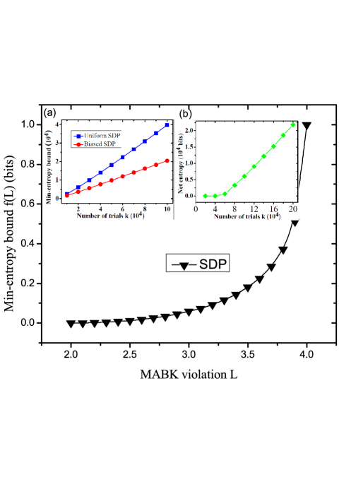
Figure 1: (Color online) Plot of the function $f(\hat{L})$ versus violation $\hat{L}$ of the MABK inequality. The function is calculated through optimization based on the semi-definite programming with the details shown in the Supplemental Material. The inset (a) shows the lower bound of the min-entropy $kf(\mathcal{L}_{m}-\epsilon)-\log_{2}\frac{1}{\delta}$ versus the number of trials $k$. Here we assume an observed MABK violation lies within the interval $3.9=\mathcal{L}_{m}\leq\hat{L}<\mathcal{L}_{max}=4$ with probability $\delta$. The parameters are chosen as $\delta=0.001$ and $\epsilon^{\prime}=0.01$. The bound $kf(\mathcal{L}_{m}-\epsilon)$ depends on the input probability distribution $P(xyz)$ through the parameter $r=\min_{xyz}P(xyz)$. The blue-square line represents the bound under a uniform distribution ($P(xyz)=1/4$ for all $(x,y,z)\in\mathcal{S}$), while the red-dotted line shows the bound under a biased probability distribution with $P(011)=P(101)=P(110)=\alpha k^{-1/2}$ and $P(000)=1-3\alpha k^{-1/2}$ with $\alpha=10$. It consumes less randomness to generate a biased distribution for the input bits, so the net amount of randomness, defined as the number of output random bits minus that of the input, becomes positive when $k$ is large (typically $k$ needs to be of the order $10^{5}$). The inset (b) plots the net amount of randomness generated after $k$ trails under a biased distribution of the inputs. The parameters are the same as those in the inset (a).

We now show how to generate and certify random numbers using Majorana fermions. The key step is to generate a three-qubit entangled state and find suitable measurements that lead to violation of the MABK inequality. Majorana fermions are non-Abelian anyons, and their braiding gives nontrivial quantum operations. However, this set of operations are very restricted. First, all the gates generated by topological manipulation of Majorana fermions belong to the Clifford group, and it is impossible to use such operations alone to violate the CHSH inequality 2009Brennen . We have to consider instead the multi-qubit MABK inequality. Second, it is not obvious that one can violate the MABK inequality as well using only topological operations. There are two ways to encode a qubit using Majorana fermions, using either two quasiparticles (Majorana fermions) or four quasiparticles (see the details in the supplement). In the two-quasiparticle encoding scheme, although the braiding gates exhaust the entire two-qubit Clifford group, they cannot span the whole Clifford group for more than two qubits 2009Ahlbrecht . Furthermore, braiding Majorana fermions within each qubit cannot change the topological charge of this qubit which fixes the measurement basis. Thus, no violation of the MABK inequality can be achieved using the topological operations alone in the two-quasiparticle encoding scheme. In the four-qusiparticle encoding scheme, it is not straightforward either as braidings in this scheme only allows certain single-qubit rotations and no entanglement can be obtained due to the no-entanglement rule proved already for this encoding scheme 2006Bravyi .

Fortunately, we can overcome this difficulty by taking advantage of the non-destructive measurement of the anyon fusion, which can induce qubit entanglement 2005Bravyi . In a real physical device, the anyon fusion can be read out non-destructively through the anyon interferometry 2010Hassler . In the four-qusiparticle encoding scheme: each qubit is encoded by four Majorana fermions, with the total topological charge $0$. The qubit basis-states are represented by $|0\rangle\equiv|((\bullet,\bullet)_{\mathbf{I}},(\bullet,\bullet)_{\mathbf{I}})_{\mathbf{I}}\rangle$ and $|1\rangle\equiv|((\bullet,\bullet)_{\psi},(\bullet,\bullet)_{\psi})_{\mathbf{I}}\rangle$. Here, each $\bullet$ represents a Majorana fermion; $\mathbf{I}$ and $\psi$ represent the two possible fusion channels of a pair of Majorana fermions, with $\mathbf{I}$ standing for the vacuum state and $\psi$ denoting a normal fermion. As explained in the Supplemental Material, a topologically protected two-qubit CNOT gate can be implemented using braidings together with non-destructive measurements of the anyon fusion 2005Bravyi . To certify randomness through the MABK inequality, we need to prepare a three-qubit entangled state. For this purpose, we need in total fourteen Majorana fermions, where twelve of them are used to encode three qubits and another ancillary pair is required for implementation of the effective CNOT gates through measurement of the anyon fusion. Initially, the logical state is $|\Phi\rangle_{i}=|000\rangle$. We apply first a Hadamard gate on the qubit $1$, which can be implemented through a series of anyon braiding as shown in Fig. 2b, and then two effective CNOT gates on the logical qubits $1$, $2$, and $2,$ $3$. The final state is the standard three-qubit maximally entangled state $|\Psi\rangle_{f}=(|000\rangle+|111\rangle)/\sqrt{2}$. After $|\Psi\rangle_{f}$ is generated, the three qubits can be separated and we need only local braiding and fusion of anyons within each qubit to perform the measurements in the appropriate bases to generate random numbers and certify them through test of the MABK inequality.

To perform the measurements, we read out each qubit according to the input string $\mathcal{I}$ through nondestructive detection of the anyon fusion. If the input is $0$, we first braid the Majorana fermions to implement a Hadamard gate $H$ on this qubit (as shown in Fig. 2b), and then measure the fusion of the first two Majorana fermions within each qubit. The measurement outcome is $0$ ($1$) if the fusion result is $\mathbf{I}$ ($\psi$). If the input is $1$, we first braid the Majorana fermions to implement a $B_{23}$ gate (see Fig. 2a) on this qubit before the same readout measurement. For instance, with the the input $(x,y,z)=(0,1,1)$, we apply a Hadamard gate to the first qubit and $B_{23}$ gates to the second and the third qubits, followed by the nondestructive measurement of fusion of the first two Majorana fermions in each qubit. Under the state $|\Psi\rangle_{f}$, the conditional probability of the measurement outcomes $(a,b,c)$ under the measurement setting $(x,y,z)$ for these three qubits is give by

$$P(abc|xyz)=\left|\langle abc|(\mathtt{U}_{x}\mathtt{U}_{y}\mathtt{U}_{z})|\Psi\rangle_{f}\right|^{2},$$ (5)

where $\mathtt{U}_{0}=H$ and $\mathtt{U}_{1}=B_{23}$. With this conditional probability, we find the expected value of $\hat{L}$ defined in Eqs. (1,2) is $\hat{L}=4$, achieving the maximum quantum violation of the MABK inequality. All the steps for measurements and state preparation are based on the topologically protected operations such as anyon braiding or nondestructive detection of the anyon fusion, so the scheme here is intrinsically fault-tolerant and we should get the ideal value of $\hat{L}=4$ if the Majorana fermions can be manipulated at will in experiments. Such a large violation perfectly certifies genuine randomness of the measurement outcomes.

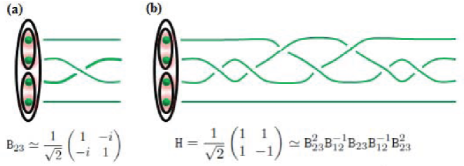
Figure 2: (Color online) Illustration of the encoding scheme for a logic qubit using Majorana fermions and two single-qubit operations that can be implemented through anyon braiding. Each qubit is encoded by four Majorana fermions. (a)A counterclockwise braiding of Majorana fermions $2$ and $3$ implements a unitary gate $\mathtt{B}_{23}$ on the corresponding qubit. (b) Implementation of the Hadamard gate through composition of anyon braiding. In both (a) and (b), time flows from left to right and $\simeq$ means equal up to an irrelevant overall phase.

In summary, we have shown that genuine number numbers can be generated and certified through topologically manipulation of Majorana fermions, a kind of anyonic excitations in engineered materials. Such a protocol is intrinsically fault-tolerant. Given the rapid experimental progress on realization of Majorana fermions in real materials 2012Mourik ; 2012Wang , this protocol offers a promising prospective for application of these topological particles in an important direction of cryptography with broad implications in science and engineering.

We thank Y. H. Chan, J. X. Gong, and E. Lichko for discussions. This work was supported by the NBRPC (973 Program) 2011CBA00300 (2011CBA00302), the IARPA MUSIQC program, the ARO and the AFOSR MURI program.

I Supplementary information: Fault Tolerant Quantum Random Number Generator Certified by Majorana Fermions

This supplementary information gives more details about realization of fault-tolerant quantum random number generator through topological manipulation of Majorana fermions. In Sec. I, we give the detailed proof on how to certify genuine randomness through observation of violation of the MABK inequality. In Sec. II, we summarize the topological properties of Majorana fermions and show the implementation of the necessary topological quantum gates on the logic qubits encoded with these Majorana fermions.

I.1 Randomness certified by observation of violation of the MABK inequality

In this section, we establish a link between randomness of the measurement outputs of a quantum system and violation of the MABK inequality. A link between randomness and violation of the Bell-CHSH inequality has been established in Ref. 2010Pironio ; correction . Here, we generalize the result from the two-qubit CHSH inequality to the three-qubit MABK inequality. Consider a quantum nonlocality test on three qubits. Each qubit has two settings of two-outcome measurements, denoted by $\left\{x,y,z\right\}$, respectively for the three qubits. The measurement outputs $\left\{a,b,c\right\}$ of this quantum system are characterized by the joint probability distribution $P=\{P(abc|xyz)\}$. Randomness of the outputs $\left\{a,b,c\right\}$ are quantified by the min-entropy, defined as $E_{\infty}(ABC|XYZ)=-\mathtt{log}_{2}[\max_{abc}P(abc|xyz)]$. With an experimental observation of violation $\hat{L}$ of the MABK inequality, our aim is to find a lower bound on the min-entropy

$$E_{\infty}(ABC|XYZ)\geq f(\hat{L}).$$ (6)

This is equivalent to solving of the following optimization problem 2010Pironio :

$$P^{\ast}(abc|xyz)=\; \max \;P(abc|xyz)$$

$$\mathtt{subject}\text{ }\mathtt{to} \;L=\hat{L}$$

$$P(abc|xyz)=\mathtt{Tr}(\rho M_{x}^{a}\otimes M_{y}^{b}\otimes M_{z}^{c})$$

where $L$ is defined in Eq.(2) of the main text and $(\rho,M_{x}^{a},M_{y}^{b},M_{z}^{c})$ constitutes a quantum realization of the Bell scenario 2011Acin . Thus, the minimal value of $E_{\infty}(ABC|XYZ)$ compatible with the MABK violation $\hat{L}$ and quantum theory is given by $E_{\infty}(ABC|XYZ)=-\mathtt{log}_{2}[\max_{abc}P^{\ast}(abc|xyz)]$. Consequently, to obtain $f(\hat{L})$ we only need to solve (I.1) for all possible input and output triplets $(x,y,z)$ and $(a,b,c)$. This can be effectively done by casting it to a semi-definite program (SDP) 1996Vandenberghe . An infinite hierarchy of conditions that need to be satisfied by all quantum correlations are introduced in Ref. 2007Navascues ; 2008Navascues ; 2009Pironio . All these conditions can be transformed to a SDP problem and the hierarchy is complete in the asymptotic limit, i.e., it guarantees existence of a quantum realization if all the conditions in the hierarchy are satisfied. Generally, conditions higher in the hierarchy are more constraining and thus better reflect the constraints in (I.1) and give a tighter lower bound. To obtain a lower bound of the min-entropy for a given MABK violation $\hat{L}$, we use the matlab toolbox SeDuMi Sturm-Sedumi and solve the SDP corresponding to the certificates between order $1$ and order $2$ 2007Navascues . The result is plotted in Fig.1 in the main text. From the figure, $f(\hat{L})$ equals zero at the classical point $\hat{L}=2$ and increases monotonously as the MABK violation $\hat{L}$ increases. For the maximal violation $\hat{L}=4$, $P^{\ast}\approx 0.5003$, corresponding to $f(\hat{L})\simeq 0.9991$ bits.

Equation (4) in the main text can be derived using arguments similar to those in Ref. 2010Pironio ; 2012Pironio . The difference is that the Bell scenario in Refs. 2010Pironio is based on the two-qubit CHSH inequality, which needs to be extended in our scheme with the three-qubit MABK inequality. Suppose we run the experiments $k$ times and denote the input and output string as $\mathcal{I}=(x_{1},y_{1},z_{1};\cdots;x_{k},y_{k},z_{k})$ and $\mathcal{O}=(a_{1},b_{1},c_{1};\cdots;a_{k},b_{k},c_{k})$, respectively. As in the main text, let $\{\mathcal{L}_{m}:0\leq m\leq m_{max}\}$ be a series of MABK violation thresholds, and denote $\mathcal{D}(m)$ the probability that the observed KCBS violation $\hat{L}$ lies in the interval $[\mathcal{L}_{m},\mathcal{L}_{m+1})$. Denote by $\mathcal{E}$ the possible classical side information an adversary may have. To derive Eq. (4) in the main text, let us first introduce the following theorem:

Theorem 1. Suppose the experiments are carried out $k$ times and each triplet of inputs $(x_{i},y_{i},z_{i})$ is generated independently with probability $P(xyz)$. Let $\delta$, $\epsilon^{\prime}>0$ be two arbitrary parameters and $r=\min\{P(xyz))\}$, then the distribution $P(\mathcal{O}\mathcal{I}\mathcal{E})$ characterizing $k$ successive use of the devices is $\epsilon^{\prime}$-close to a distribution $\mathcal{D}$ such that, either $\mathcal{D}(m)\leq\delta$ or

$$E_{\infty}(\mathcal{O}|\mathcal{I},\mathcal{E},m)_{\mathcal{D}}\geq kf(\mathcal{L}_{m}-\epsilon)+\log_{2}\delta,$$ (8)

where $\epsilon=(4+1/r)\sqrt{-2\ln\epsilon^{\prime}/k}$.

Equation (8) is equivalent to Eq. (4) in the main text. Theorem 1 tells us that the distribution $P$, which characterizes the output $\mathcal{O}$ of the device and its correlation with the input $\mathcal{I}$ and the adversary’s classical side information $\mathcal{E}$, is basically indistinguishable from a distribution $\mathcal{D}$ that will be defined below 2012Pironio . If we find that the observed MABK violation $\hat{L}$ lies in $[\mathcal{L}_{m},\mathcal{L}_{m+1})$ with a non-negligible probability, i.e., $\mathcal{D}(m)>\delta$, the entropy of the outputs $\mathcal{O}$ is guaranteed to have a positive lower bound $kf(\mathcal{L}_{m}-\epsilon)-\log_{2}\frac{1}{\delta}$, that is, the randomness of the outputs is guaranteed to be larger than $kf(\mathcal{L}_{m})$ up to epsilonic correction.

Proof. We use a procedure similar to those in Ref. 2012Pironio to prove the above theorem. Let us define a function $\mathcal{G}(L)=2^{-f(L)}$, which is concave and monotonically decreasing given by the solution of the optimization problem in Eq. (I.1) (shown in Fig. 1 of the main text). Denote by $\mathcal{O}^{n}=(a_{i},b_{i},c_{i};\cdots;a_{n},b_{n},c_{n})$ ($n\leq k$) the string of outputs before the $(n+1)$th round of experiment (similarly, $\mathcal{I}^{n}$ denotes the string of inputs). We introduce an indicator function $\chi(e)$ as: $\chi(e)=1$ if the event $e$ happens and $\chi(e)=0$ otherwise. Consider the following random variable

$$\hat{L}_{i}=\sum_{abc;(x,y,z)\in\mathcal{S}}\tau(x,y,z)\Lambda(a,b,c)\frac{\chi(a_{i}=a,b_{i}=b,c_{i}=c;x_{i}=x,y_{i}=y,z_{i}=z)}{P(xyz)},$$ (9)

where $\mathcal{S}$ and $\tau(x,y,z)$ are defined in the main text, and $\Lambda(a,b,c)=1$ if $a+b+c$ is $\mathtt{even}$ and $\Lambda(a,b,c)=-1$ if $a+b+c$ is $\mathtt{odd}$. It is easy to check that Eq.(9) reduces to the MABK expression (2) in the main text and the expectation value of $\hat{L}_{i}$ conditional on the past $W^{i}$ is equal to $L(W^{i})$, i.e., $\mathbb{E}(\hat{L}_{i}|W^{i})=L(W^{i})$. We use $\mathcal{W}^{i}\equiv(\mathcal{O}^{i-1}\mathcal{I}^{i-1}\mathcal{E})$ to denote all the events before the $i$th round of experiment and the possible adversary’s classical side information. The estimator of the MABK violation can be defined as: $\hat{L}=\frac{1}{k}\sum_{i=1}^{k}\hat{L}_{i}$. With these notations, first we introduce two lemmas for proof of the main theorem.

Lemma 1. For any given parameter $\epsilon^{\prime}>0$, let $\epsilon=(4+1/r)\sqrt{-2\ln\epsilon^{\prime}/k}$ and $S_{\epsilon}=\{(\mathcal{O},\mathcal{I},\mathcal{E})|\frac{1}{k}\sum_{i=1}^{k}\mathbb{E}(\hat{L}_{i}|W^{i})\geq\hat{L}(\mathcal{O},\mathcal{I})-\epsilon\}$, then we have:

(i) for any $(\mathcal{O},\mathcal{I},\mathcal{E})\in S_{\epsilon}$,

$$P(\mathcal{O}|\mathcal{I}\mathcal{E})\leq\mathcal{G}^{k}(\hat{L}(\mathcal{O},\mathcal{I})-\epsilon).$$ (10)

(ii)

$$\mathtt{Pr}(S_{\epsilon})=\sum_{(\mathcal{O},\mathcal{I},\mathcal{E})\in S_{\epsilon}}P(\mathcal{O},\mathcal{I},\mathcal{E})\geq 1-\epsilon^{\prime}.$$ (11)

Proof. According to the Bayes’ rule and the fact that the response of a system does not depend on the future inputs and outputs, we have:

$$P(\mathcal{O}|\mathcal{I}\mathcal{E}) = \prod_{i=1}^{k}P(a_{i}b_{i}c_{i}|\mathcal{O}^{i-1}\mathcal{I}^{i}\mathcal{E})$$ (12)

$$= \prod_{i=1}^{k}P(a_{i}b_{i}c_{i}|x_{i}y_{i}z_{i}\mathcal{W}^{i})$$

From the solution to the optimization problem in Eq. (I.1), the probability $P(a_{i}b_{i}c_{i}|x_{i}y_{i}z_{i}\mathcal{W}^{i})$ is bounded by a function of the MABK violation $L(W^{i})$: $P(a_{i}b_{i}c_{i}|x_{i}y_{i}z_{i}\mathcal{W}^{i})\leq\mathcal{G}(L(W^{i}))$. Thus, we have:

$$P(\mathcal{O}|\mathcal{I}\mathcal{E}) \leq \prod_{i=1}^{k}\mathcal{G}(L(W^{i}))$$ (13)

$$\leq \mathcal{G}^{k}(\frac{1}{k}\mathbb{E}(\hat{L}_{i}|W^{i}))$$

$$\leq \mathcal{G}^{k}(\hat{L}(\mathcal{O},\mathcal{I})-\epsilon).$$

Here, to obtain the second inequality, we have used the equality $\mathbb{E}(\hat{L}_{i}|W^{i})=L(W^{i})$ and the fact that $\mathcal{G}$ is logarithmically concave and monotonically decreasing. The third inequality is obtained from the definition of $S_{\epsilon}$ and the fact that $\mathcal{G}$ is decreasing. To get Eq. (11), we can define another random variable $M^{q}=\sum_{i=1}^{q}(\hat{L}_{i}-\mathbb{E}(\hat{L}_{i}|W^{i}))$. Then it is easy to verify that (i) $|M^{q}|\leq 2q/r<\infty$, (ii) $|\hat{L}_{i}-L(W^{i})|\leq|\hat{L}_{i}|+|L(W^{i})|\leq\frac{1}{r}+4$, and (iii) $\mathbb{E}(M^{q+1}|W^{q})=M^{q}$. Thus, the sequence $\{M^{q}:q\geq 1\}$ is a martingale process 2001Grimmett-Book . Applying the Azuma-Hoeffding inequality $P(M^{q}\geq k\epsilon)\leq\exp(-\frac{(k\epsilon)^{2}}{2k(1/r+4)^{2}})$ 1967Azuma ; 1960Hoeffding ; 2001Grimmett-Book , we have

$$P\left(\frac{1}{k}\sum_{i=1}^{k}\mathbb{E}(\hat{L}|W^{i})\leq\frac{1}{k}\sum_{i=1}^{k}\hat{L}_{i}-\epsilon\right)\leq\epsilon^{\prime},$$ (14)

where $\epsilon=(4+1/r)\sqrt{-2\ln\epsilon^{\prime}/k}$. Equation (14) combined with the definition of $S_{\epsilon}$ gives Eq. (11). Lemma 1 is thus proved.

In the above proof, we only considered the case that the random variable sequence $\mathcal{O}$ takes values in the output space $\mathbb{S}^{k}=\{-1,1\}^{k}$. As in Ref. 2012Pironio , we can extend the range of $\mathcal{O}$ to include “abort-output” $\bot$, and view $\mathcal{O}$ as an element of $\mathbb{S}^{k}\cup\bot$ with $P(\mathcal{O}|\mathcal{I}\mathcal{E})=0$ if $\mathcal{O}=\bot$. The physical meaning of $\bot$ is that when $\bot$ is produced by the device, then no MABK violation has been obtained and no randomness is certified.

Lemma 2. There exists a probability distribution $\mathcal{D}=\{\mathcal{D}(\mathcal{O},\mathcal{I},\mathcal{E})\}$, which is $\epsilon^{\prime}$-close to $P=\{P(\mathcal{O},\mathcal{I},\mathcal{E})\}$, i.e., $d(\mathcal{D},P)=\frac{1}{2}\sum_{\mathcal{O},\mathcal{I},\mathcal{E}}|P(\mathcal{O},\mathcal{I},\mathcal{E})-\mathcal{D}(\mathcal{O},\mathcal{I},\mathcal{E})|\leq\epsilon^{\prime}$, and satisfies the following condition

$$\mathcal{D}(\mathcal{O}|\mathcal{I},\mathcal{E})\leq\mathcal{G}^{k}(\hat{L}(\mathcal{O},\mathcal{I})-\epsilon),$$ (15)

for all $(\mathcal{O},\mathcal{I},\mathcal{E})$ such that $\mathcal{O}\neq\bot$.

Proof. We show how to construct a probability distribution satisfying the above two conditions. To this end, we introduce $\mathcal{D}(\mathcal{O},\mathcal{I},\mathcal{E})=P(\mathcal{I})P(\mathcal{E})\mathcal{D}(\mathcal{O}|\mathcal{I},\mathcal{E})$. $\mathcal{D}(\mathcal{O}|\mathcal{I},\mathcal{E})$ is defined as:

$$\mathcal{D}(\mathcal{O}|\mathcal{I},\mathcal{E})=\left\{\begin{array}[]{cc}P(\mathcal{O}|\mathcal{I},\mathcal{E}),&\mathtt{if}\;(\mathcal{O},\mathcal{I},\mathcal{E})\in S_{\epsilon}\\ 0,&\quad\quad\mathtt{if}\;\mathcal{O}\neq\bot\;\mathtt{and}\;(\mathcal{O},\mathcal{I},\mathcal{E})\notin S_{\epsilon}\\ 1-\sum_{(\mathcal{O},\mathcal{I},\mathcal{E})\notin S_{\epsilon}}P(\mathcal{O}|\mathcal{I},\mathcal{E})&\;\mathtt{otherwise}\end{array}\right.$$ (16)

Then by Lemma 1, it is straightforward to get that the distribution $\mathcal{D}$ satisfies Eq. (15) for all $(\mathcal{O},\mathcal{I},\mathcal{E})$ with $\mathcal{O}\neq\bot$. The distance between $P$ and $\mathcal{D}$ can be calculated as:

$$d(\mathcal{D},P) = \frac{1}{2}\sum_{\mathcal{O},\mathcal{I},\mathcal{E}}|P(\mathcal{O},\mathcal{I},\mathcal{E})-\mathcal{D}(\mathcal{O},\mathcal{I},\mathcal{E})|$$

$$= \frac{1}{2}\sum_{\mathcal{I},\mathcal{E}}P(\mathcal{I},\mathcal{E})\sum_{\mathcal{O}}|P(\mathcal{O}|\mathcal{I},\mathcal{E})-\mathcal{D}(\mathcal{O}|\mathcal{I},\mathcal{E})|$$

$$= \frac{1}{2}[\sum_{(\mathcal{O},\mathcal{I},\mathcal{E})\notin\mathcal{T}_{\epsilon}}P(\mathcal{O},\mathcal{I},\mathcal{E})+1-\sum_{(\mathcal{O},\mathcal{I},\mathcal{E})\in\mathcal{T}_{\epsilon}}P(\mathcal{O},\mathcal{I},\mathcal{E})]$$

$$\leq \epsilon^{\prime}.$$

This proves Lemma 2.

With Lemma 2, now the proof of Theorem 1 becomes straightforward. Define a subset of the outputs as $\mathcal{X}_{m}=\{\mathcal{O}|\mathcal{O}\neq\bot\;\mathtt{and}\;\mathcal{L}_{m}\leq\hat{L}<\mathcal{L}_{m+1}\}$ and let $\mathcal{D}(\mathcal{O},\mathcal{I},\mathcal{E}|m)$ denote the distribution of $\mathcal{O},\mathcal{I},\mathcal{E}$ conditioned on a particular value of $m$, then we have:

$$E_{\infty}(\mathcal{O}|\mathcal{I},\mathcal{E},m)_{\mathcal{D}} \equiv -\mathtt{log}_{2}\sum_{\mathcal{I},\mathcal{E}}[\max_{\mathcal{O}}\mathcal{D}(\mathcal{O},\mathcal{I},\mathcal{E}|m)]$$

$$= -\mathtt{log}_{2}\sum_{\mathcal{I},\mathcal{E}}\mathcal{D}(\mathcal{I},\mathcal{E}|m)[\max_{\mathcal{O}}\mathcal{D}(\mathcal{O}|\mathcal{I},\mathcal{E},m)]$$

$$= -\mathtt{log}_{2}\sum_{\mathcal{I},\mathcal{E}}\mathcal{D}(\mathcal{I},\mathcal{E}|m)\frac{1}{\mathcal{D}(m|\mathcal{I},\mathcal{E})}\max_{\mathcal{O}\in\mathcal{X}_{m}}\mathcal{D}(\mathcal{O}|\mathcal{I},\mathcal{E})$$

$$\geq -\mathtt{log}_{2}\sum_{\mathcal{I},\mathcal{E}}\mathcal{D}(\mathcal{I},\mathcal{E}|m)\frac{\mathcal{G}^{k}(\mathcal{L}_{m}-\epsilon)}{\mathcal{D}(m|\mathcal{I},\mathcal{E})}$$

$$= -\mathtt{log}_{2}\sum_{\mathcal{I},\mathcal{E}}\frac{\mathcal{D}(\mathcal{I},\mathcal{E})}{\mathcal{D}(m)}\mathcal{G}^{k}(\mathcal{L}_{m}-\epsilon)$$

$$= kf(\mathcal{L}_{m}-\epsilon)-\log_{2}\frac{1}{\mathcal{D}(m)}.$$

Here we have used the Bayes’ rule in the first, second and the fourth equalities and Eq. (15) from Lemma 2 in the third inequality; for the last equality, the equation $f=-\log_{2}\mathcal{G}$ is used. The last equality immediately leads to the claim in Theorem 1. This concludes the proof.

It is worthwhile to clarify that in deriving Eq. (8) we have made the following four assumptions 2010Pironio ; 2012Pironio : (i) the system can be described by quantum theory; (ii) the inputs at the $j$th trial $(x_{j},y_{j},z_{j})$ are chosen randomly and their values are revealed to the systems only at step $j$; (iii) the three qubits are separated and non-interacting during each measurement step. (iv) the possible adversary has only classical side information. There are no constraints on the states, measurements, or the Hilbert space. Moreover, there is even no requirement that the system behaves identically and independently for each trial. In particular, the system could have an internal memory (classical or quantum) so that the results of the $j$th trial depend on the previous $j-1$ trials.

We also note that there is a significant difference between the two-qubit scenario in Ref. 2010Pironio and our three-qubit scenario here. In the two-qubit case, the randomness can be certified by the no-signalling conditions as well without the assumption of quantum mechanics. However, in our three-qubit scenario, the no-signalling conditions are not sufficient to certify randomness. Actually, we have numerically checked that even for the maximal possible MABK violation $\hat{L}_{max}=4$, $P^{\ast}(abc|xyz)$ can be equal to the unity for certain $(a,b,c)$ and $(x,y,z)$ if only the no-signalling conditions are imposed, which cannot certify any randomness. A possible reason for this difference is that the MABK inequality only contains four out of eight possible correlations. In other words, the input choices $\mathcal{S}$ is only a subset of $\{(x,y,z)|x,y,z=0,1\}$. As a result, the no-signalling constraints become less effective.

I.2 Encoding and operation of qubits by topological manipulation of Majorana fermions

In this section, we discuss in detail how to control the logical qubits encoded with Majorana fermions. The fusion rule of Majorana fermions is of the Ising type: $\tau\times\tau\sim\mathbf{I}+\psi$, where $\tau$, $\mathbf{I}$, and $\psi$ stand for a Majorana fermion, the vacuum state, and a normal fermion, respectively. Generally, there are two encoding schemes. The first scheme encodes each logical qubit into a pair of Majorana fermions (two-quasiparticle encoding). When the pair fuse to a vacuum state $\mathbf{I}$, we say that the qubit is in state $|0\rangle$; and when they fuse to $\psi$, the state is $|1\rangle$. There is also an ancillary pair, which soak up the extra $\psi$ if necessary to maintain the constraint that the total topological charge must be $0$ for the entire system 2006Georgiev ; 2009Ahlbrecht . In this encoding scheme, braiding operations of Majorana fermions exhaust the entire two-qubit Clifford group. However, for three or more qubits, not all Clifford gates could be implemented by braiding. The embedding of the two-qubit SWAP gate into a $n$-qubit system cannot be implemented by braiding 2009Ahlbrecht . In the two-quasiparticle encoding scheme, no violation of the MABK inequality can be obtained as we cannot change the measurement basis through local braiding of Majorana fermions within each logic qubit.

As we mentioned in the main text, we use the four-quasiparticle encoding scheme where the qubit basis-states are represented by $|0\rangle=|((\bullet,\bullet)_{\mathbf{I}},(\bullet,\bullet)_{\mathbf{I}})_{\mathbf{I}}\rangle$ and $|1\rangle=|((\bullet,\bullet)_{\psi},(\bullet,\bullet)_{\psi})_{\mathbf{I}}\rangle$. Let us first consider braiding operations of Majorana fermions within each logic qubit. Consider four Majorana operators $c_{i}$ $(i=1,2,3,4)$ in one logic qubit, which satisfy $c_{i}^{\dagger}=c_{i}$, $c_{i}^{2}=1$ and the anti-commutation relation $\{c_{i},c_{j}\}=2\delta_{ij}$. The Pauli operators in the computational basis can be expressed as 2010Hassler :

$$\sigma^{x}=-ic_{2}c_{3},\quad\sigma^{y}=-ic_{1}c_{3},\quad\sigma^{z}=-ic_{1}c_{2}.$$ (19)

Unitary operations can be implemented by counterclockwise exchange of two Majorana fermions $j<j^{\prime}$:

$$\mathtt{B}_{jj^{\prime}}=e^{(i\pi/4)(ic_{j}c_{j^{\prime}})}.$$ (20)

Specifically, we can write down the three basic braiding operators in the computational basis:

$$\mathtt{B}_{12}=\mathtt{B}_{34}\simeq\left(\begin{matrix}1&0\\ 0&i\end{matrix}\right),\;\mathtt{B}_{23}\simeq\frac{1}{\sqrt{2}}\left(\begin{matrix}1&-i\\ -i&1\end{matrix}\right),$$ (21)

where $\simeq$ means that we ignore an unimportant overall phase. Using these basic braiding operators, a single-qubit Hadamard gate can be implemented as $\mathtt{H}=\frac{1}{\sqrt{2}}\left(\begin{matrix}1&1\\ 1&-1\end{matrix}\right)\simeq\mathtt{B}_{23}^{2}\mathtt{B}_{12}^{-1}\mathtt{B}_{23}\mathtt{B}_{12}^{-1}\mathtt{B}_{23}^{2}$. The corresponding braidings are shown in Fig.2 of the main text. Note that the set of operations implemented through composition of $\mathtt{B}_{12}$ and $\mathtt{B}_{23}$ are still very limited, however, it is fortunate that $\mathtt{B}_{23}$ and $\mathtt{H}$ give all the gates that we need for change of the measurement bases in test of the MABK inequality. As shown in the main text, we actually get maximum quantum violation of the MABK inequality by randomly choosing either a $\mathtt{B}_{23}$ or an $\mathtt{H}$ gate on each logic qubit before measurement of the anyon fusion.

With only braiding operations of Majorana fermions, no entangling gate can be achieved for logic qubits in the four-quasiparticle encoding scheme due to the no-entanglement rule proved in Ref. 2006Bravyi . In order to overcome this problem, we need assistance from another kind of topological manipulation: nondestructive measurement of the anyon fusion, which can be implemented through the anyon interferometry as proposed in Ref. 2010Hassler . Suppose that we have eight Majorana modes $c_{1},c_{2},\ldots,c_{8}$, where the first (last) four modes encode the control (target) qubit, respectively. As shown in Ref. 2002Bravyi ; 2005Bravyi , a two-qubit controlled phase flip gate $\Lambda(\sigma^{z})$ can be implemented through the following identity:

$$\Lambda(\sigma^{z})=e^{-(\pi/4)c_{3}c_{4}}e^{-(\pi/4)c_{5}c_{6}}e^{(i\pi/4)c_{4}c_{3}c_{5}c_{6}}e^{i\pi/4}.$$ (22)

Note that the first two operations in Eq. (22) can be directly implemented by braiding operations. The key step is to implement the operation $e^{(i\pi/4)c_{4}c_{3}c_{5}c_{6}}$. To this end, we use another ancillary pair of Majorana fermions $c_{9}$ and $c_{10}$. We measure fusion of the four Majorana modes $c_{4}c_{3}c_{6}c_{9}$. The outcome is $\pm 1$, corresponding to either a vacuum state ($+1$) or a normal fermion ($-1$) . The corresponding projector is given by $\Pi_{\pm}^{(4)}=\frac{1}{2}(1\pm c_{4}c_{3}c_{6}c_{9})$. Then, we similarly measure fusion of the Majorana modes (operator) $-ic_{5}c_{9}$, with the project denoted by $\Pi_{\pm}^{(2)}=\frac{1}{2}(1\mp ic_{5}c_{9})$ corresponding to the measurement outcomes $\pm 1$. We have the following relation 2002Bravyi ; 2005Bravyi :

$$e^{(i\pi/4)c_{4}c_{3}c_{5}c_{6}}=2\displaystyle\sum\limits_{\eta,\zeta=\pm}U_{\eta\zeta}\Pi_{\eta}^{(2)}\Pi_{\zeta}^{(4)},$$ (23)

where $U_{++}=e^{(\pi/4)c_{5}c_{10}}$, $U_{+-}=ie^{(\pi/2)c_{4}c_{3}}e^{(\pi/2)c_{5}c_{6}}e^{(\pi/4)c_{5}c_{10}}$, $U_{-+}=ie^{(\pi/2)c_{4}c_{3}}e^{(\pi/2)c_{5}c_{6}}e^{-(\pi/4)c_{5}c_{10}}$, and $U_{--}=e^{-(\pi/4)c_{5}c_{10}}$. All the gates $U_{\eta\zeta}$ can be implemented through one or several braiding operations of Majorana fermions. So this identity shows that an effective controlled phase flip gate can be implemented on logic qubits through a combination of anyon braiding and measurement of anyon fusion. Depending on the measurement outcomes $(\zeta,\eta)$ of $c_{4}c_{3}c_{6}c_{9}$ and $-ic_{5}c_{9}$, one can always apply a suitable correction operator $U_{\eta\zeta}$ to obtain the desired operation $e^{(i\pi/4)c_{4}c_{3}c_{5}c_{6}}$. With controlled phase flip gates, one can easily realize quantum controlled-NOT (CNOT) gate with assistance from the Hadamard operations that can be implemented through the anyon braiding. With CNOT and Hadamard gates, we can then prepare the maximally entangled three-qubit state as required for test of quantum violation of the MABK inequality.

References

- (1) E. Majorana, Nuovo Cimento 14, 171 (1937).
- (2) F. Wilczek, Nat. Phys. 5, 614 (2009).
- (3) A. Stern, Nature 464, 187 (2010).
- (4) C. Nayak, S. H. Simon, A. Stern, M. Freedman, and S. Das Sarma, Rev. Mod. Phys. 80, 1083 (2008).
- (5) L. Fu and C. L. Kane, Phys. Rev. Lett. 100, 096407 (2008).
- (6) A. Kitaev, Ann. Phys. (N. Y.) 321, 2 (2006).
- (7) N. Read and D. Green, Phys. Rev. B 61, 10267 (2000).
- (8) J. D. Sau, R. M. Lutchyn, S. Tewari, and S. DasSarma, Phys. Rev. Lett. 104, 040502 (2010).
- (9) R. M. Lutchyn, J. D. Sau, and S. DasSarma, Phys. Rev. Lett. 105, 077001 (2010).
- (10) Y. Oreg, G. Refael, and F. von Oppen, Phys. Rev. Lett. 105, 177002 (2010).
- (11) M. X. Wang, et al. Science 336, 52-55 (2012).
- (12) V. Mourik, et al., Science 336, 1003 (2012).
- (13) N. D. Mermin, Phys. Rev. Lett. 65, 1838 (1990).
- (14) M. Ardehali, Phys. Rev. A 46, 5375 (1992).
- (15) A. V. Belinskii and D. N. Klyshko, Phys. Usp. 36, 653 (1993).
- (16) J. Ackermann, et al. Comput. Phys. Commun. 140, 293 (2001).
- (17) P. F. Hultquist, Simulation. 57, 258 (1991).
- (18) S. J. Tu and E. Fischbach, Phys. Rev. E 67, 016113 (2003).
- (19) S. Pironio, et al. Nature 464, 1021 (2010).
- (20) M. Isida and Y. Ikeda, Ann. Inst. Stat. Math. 8, 119 (1956).
- (21) K. Svozil, Phys. Lett. A 143, 433 (1990).
- (22) J. G. Rarity, M. P. C. Owens, and P. R. Tapster, Journal of Modern Optics 41, 2435 (1994).
- (23) T. Jennewein, et al. Rev. Sci. Instrum. 71, 1675 (2000).
- (24) J. Clauser, F. M.Horne, A. A. Shimony, and R. A. Holt, Phys. Rev. Lett. 23, 880 (1969).
- (25) Colbeck, R. Quantum and Relativistic Protocols for Secure Multi-Party Computation. PhD dissertation, Univ. Cambridge (2007).
- (26) G. K. Brennen, S. Iblisdir, J. K. Pachos, and J. K. Slingerland, New J. of Phys. 11, 103023 (2009).
- (27) R. Koenig, R. Renner, and C. Schaffner, IEEE Trans. Inf. Theory 55, 4337 (2009).
- (28) S. Pironio and S. Massar, arXiv: 1111.6056v4.
- (29) L. Vandenberghe and S. Boyd, SIAM Rev. 38, 49 (1996).
- (30) N. Nisan and A. Ta-Shma, J. Comput. Syst. Sci. 58, 148 (1999).
- (31) A. Ahlbrecht, L. S. Georgiev,and R. F. Werner, Phys. Rev. A 79, 032311 (2009).
- (32) S. Bravyi, Phys. Rev. A 73, 042313 (2006).
- (33) S. Bravyi and A. Y. Kitaev, Phys. Rev. A 71, 022316 (2005).
- (34) F. Hassler, A. R. Akhmerov, C. Y. Hou, and C. W. J. Beenakker, New J. of Phys. 12 125002 (2010).
- (35) The theoretical results in Ref. 2010Pironio were improperly formulated, and the inaccuracies in formulation were corrected in the recent Refs. 2012Pironio and 2012Fehr .
- (36) A. Acín, S. Massar, and S. Pironio, arXiv: 1107.2754.
- (37) M. Navascues, S. Pironio, and A. Acin, Phys. Rev. Lett. 98, 010401 (2007).
- (38) M. Navascues, S. Pironio, and A. Acin, New J. Phys. 10, 073013 (2008).
- (39) S. Pironio, M. Navascues, and A. Acin, arXiv: 0903.4368.
- (40) Sturm, J. SeDuMi, a MATLAB toolbox for optimization over symmetric cones. http://sedumi.mcmaster.ca.
- (41) G. Grimmett and D. Stirzaker, Probability and Random Processes (Oxford University Press, Oxford, 2001).
- (42) W. Hoeffding, Journal of the American Statistical Association 58, 13 (1963).
- (43) K. Azuma, Tohoku Mathematical Journal 19, 357(1967).
- (44) L. S. Georgiev, Phys. Rev. B 74, 235112 (2006).
- (45) S. B. Bravyi and A. Y. Kitaev, Ann. Phys. 298 210 (2002).
- (46) S. Fehr, R. Gelles, and C. Schaffner, arXiv: 1111.6052v3.