Fragment-based Time-dependent Density-functional Theory

Abstract

Using the Runge-Gross theorem that establishes the foundation of Time-dependent Density Functional Theory (TDDFT) we prove that for a given electronic Hamiltonian, choice of initial state, and choice of fragmentation, there is a unique single-particle potential (dubbed time-dependent partition potential) which, when added to each of the pre-selected fragment potentials, forces the fragment densities to evolve in such a way that their sum equals the exact molecular density at all times. This uniqueness theorem suggests new ways of computing time-dependent properties of electronic systems via fragment-TDDFT calculations. We derive a formally exact relationship between the partition potential and the total density, and illustrate our approach on a simple model system for binary fragmentation in a laser field.

Time-dependent density functional theory (TDDFT) Runge and Gross (1984); Ullrich (2012) allows one to predict, in principle, the evolution of the non-relativistic density $n({\bf r}t)$ of a system of interacting electrons subject to a time-dependent external potential $v({\bf r}t)$. Given an initial wave function, the time-dependent electron density determines the external potential up to a time-dependent constant (Runge-Gross theorem [RG] Runge and Gross (1984)) and the density may be found by solving the time-dependent Kohn-Sham (TDKS) equations. These equations make it possible to perform practical calculations to propagate the electronic density and its related quantities such as linear response functions. Due to its wide range of applications, TDDFT is expected to continue being a workhorse in the coming years for chemistry, physics, and materials engineering Burke et al. (2005).

Although the computational cost of TDKS calculations is low compared to that of other many-body techniques, new ideas are needed to enable the study of larger systems with improved efficiency and accuracy. For the ground-state problem, ‘divide-and-conquer’ fragmentation techniques have been developed Yang (1991) and applied successfully through the use of readily-available parallel computers. Related strategies have also been developed recently for the time-dependent problem within TDDFT Severo Pereira Gomes and Jacob (2012). For example, Casida and Wesołowski (2004) introduced a methodology to perform time-dependent calculations within frozen-density embedding theory. It has been shown that this method yields better results than “supermolecular” techniques in some cases Fradelos et al. (2011); Neugebauer et al. (2005). Other extensions include linear-response TDDFT for molecules in solvents Iozzi et al. (2004) and TDDFT for interacting chromophores Hsu et al. (2001). Also, time-dependent calculations within subsystem-DFT have been reported (see Neugebauer (2010) and references therein). In subsystem-DFT, the density of the system is split into densities of localized subsystems. Then the Kohn-Sham kinetic energy of the total system is truncated, and the energy functional is approximated by a functional of the subsystem densities; its minimization leads to Kohn-Sham equations for each subsystem. Neugebauer formulated this theory within linear response in the frequency domain and showed that it yields results consistent with conventional TDDFT Neugebauer (2007). For the case of dissipative dynamics, Zhou et al. (Yuen-Zhou et al., 2010) showed how the RG theorem can be applied and Kohn-Sham equations developed for open systems given an initial state, memory kernel, and system-bath correlation.

Among density-based ground-state fragmentation techniques, Partition Density Functional Theory (PDFT) Elliott et al. (2010) is a reformulation of Density Functional Theory that allows one to find the solution to the KS equations without solving the total molecular problem directly. The idea is to partition the external potential into an arbitrary number of fragment potentials. The total energy of the isolated systems is minimized under the constraint that the fragment densities sum to the correct molecular density. The Lagrange multiplier associated with the constraint (i.e. the partition potential) can be found by inversion if the total density is known Cohen and Wasserman (2007), or via the self-consistent procedure of Ref. Elliott et al. (2010) if it is not. Every fragment is subject to the same partition potential. In contrast with quantum mechanical embedding theories (except for the latest version of quantum embedding Huang et al. (2011)) and with subsystem-DFT, this potential is global and unique Cohen and Wasserman (2006). The set of fragment densities obtained for a given choice of external-potential partitioning is also unique. As Pavanello (2013) recently suggested, this uniqueness feature of PDFT makes it a suitable candidate to simplify the formulation of subsystem-DFT. This letter reports on foundational work for such developments. We extend PDFT to the time-dependent regime and show how the time-dependent external field can be partitioned. A new potential termed the time-dependent partition potential is introduced in the formalism in order to represent the exact time-dependent electronic density.

To extend PDFT to the time-dependent domain we recall that there is no minimum principle from which the TDKS equations can be derived Rajagopal (1996); Vignale (2008). In view of this, we follow a deductive approach to define our TDKS equations. Our goal is to provide a fragment-based solution to the Liouville equation (we use atomic units throughout)

$$i\frac{\partial\hat{\Gamma}\left(t\right)}{\partial t}=\left[\hat{H}_{v}(t),\hat{\Gamma}(t)\right].$$ (1)

If $\hat{\Gamma}$ is a pure density matrix then Eq. (1) is equivalent to the time-dependent Schrödinger equation. We suppose that the initial state $\hat{\Gamma}(t_{0})$ is given. In standard DFT notation, the Hamiltonian is given by $\hat{H}_{v}(t)=\hat{T}+\hat{V}_{ee}+\int\text{d}^{3}\mathbf{r}~{}v\left(\mathbf{r}t\right)\hat{n}\left(\mathbf{r}\right)$. It is convenient to express the external potential $v({\bf r}t)$ as the sum of the potential $\tilde{v}({\bf r})$ due to the $M$ nuclei $\tilde{v}({\bf r})=-\sum_{\alpha}^{M}Z_{\alpha}/|{\bf r}-{\bf R}_{\alpha}|$, which is not explicitly time-dependent, and an additional potential $v_{E}({\bf r}t)$ containing all of the explicit time-dependence due to external fields:

$$v({\bf r}t)=\tilde{v}({\bf r})+v_{E}({\bf r}t)$$ (2)

Our task is to divide the quantum system into $N_{f}$ fragments of interacting electrons. This is done by assigning an external potential $v_{\alpha}({\bf r}t)$, Hamiltonian $\hat{H}_{\alpha}(t)$, and initial state $\hat{\Gamma}_{\alpha}(t_{0})$ to each fragment. Out of the infinitely many ways to choose the fragment potentials, there are at least two cases that are physically relevant: (i) Direct partitioning of the time-dependent external potential in analogy to ground-state PDFT: $v(\mathbf{r}t)=\sum_{\alpha}^{N_{f}}v_{\alpha}(\mathbf{r}t)$. For example, if $N_{f}=M$, there are cases of interest where we could define $v_{\alpha}(\mathbf{r}t)=-Z_{\alpha}/\left|\mathbf{r}-\mathbf{R}_{\alpha}(t)\right|$. In such cases, the electronic density of fragment $\alpha$ would be an output variable of the dynamics of nucleus $\alpha$. In general, however, we find option (ii) to be more convenient: Fragment the static potential only,

$$\tilde{v}({\bf r})=\sum_{\alpha}\tilde{v}_{\alpha}({\bf r})~{}~{},$$ (3)

and define the time-dependent fragment potential $v_{\alpha}({\bf r}t)$ by adding the total time-dependent potential $v_{E}({\bf r}t)$ to each of the $\tilde{v}_{\alpha}({\bf r}t)$’s:

$$v_{\alpha}(\mathbf{r}t)=\tilde{v}_{\alpha}(\mathbf{r})+v_{E}(\mathbf{r}t)~{}.$$ (4)

Now define the many-electron fragment-$\alpha$ Hamiltonian as

$$\hat{H}_{\alpha}(t)=\hat{T}+\hat{V}_{ee}+\int\text{d}^{3}\mathbf{r}\,\left[v_{\alpha}(\mathbf{r}t)+v_{p}(\mathbf{r}t)\right]\hat{n}(\mathbf{r})~{}.$$ (5)

The evolution of the state of this particular fragment is governed by the Liouville equation

$$i\frac{\partial}{\partial t}\,\hat{\Gamma}_{\alpha}(t)=\left[\hat{H}_{\alpha}(t),\hat{\Gamma}_{\alpha}(t)\right]~{}.$$ (6)

The time-dependent electronic density of fragment $\alpha$ is given by $n_{\alpha}({\bf r}t)=\mathrm{Tr}\{\hat{\Gamma}_{\alpha}(t)\hat{n}(\mathbf{r})\}$ and the time-dependent partition potential $v_{p}({\bf r}t)$ of Eq. (5) is defined by requiring that the sum of fragment densities reproduce the total molecular density at all times:

$$\sum_{\alpha=1}^{N_{f}}n_{\alpha}(\mathbf{r}t)=n(\mathbf{r}t)~{}~{}.$$ (7)

Just like traditional TDDFT is based on a one-to-one mapping between the Kohn-Sham potential $v_{s}(\mathbf{r}t)$ and the electronic density $n({\bf r}t)$, we now prove an analogous one-to-one mapping between $n({\bf r}t)$ and $v_{p}({\bf r}t)$. The latter is therefore sharply defined by Eqs. (1)-(7).

Theorem 1.

For a given set of initial states $\{\hat{\Gamma}_{\alpha}(t_{0})\}$, the map between the density and the partition potential is invertible up to a time-dependent constant in the potential.

Proof.

The proof uses the Runge-Gross theorem Runge and Gross (1984), and is analogous to it. Suppose there is a minimum integer $k\geq 0$ such that

$$\frac{\partial^{m}}{\partial t^{m}}[v_{p}^{\prime}(\mathbf{r}t)-v_{p}(\mathbf{r}t)]\Big{|}_{t=t_{0}}\begin{cases}=\mathrm{Constant}\quad m<k\\ \neq\mathrm{Constant}\quad m=k~{}.\end{cases}$$ (8)

Also assume that $v_{p}$ and $v_{p}^{\prime}$ have the associated densities $\{n_{\alpha}\}$ and $\{n_{\alpha}^{\prime}\}$ correspondingly. Suppose $\hat{H}_{\alpha}(t)$ and $\hat{H}_{\alpha}^{\prime}(t)$ are the Hamiltonians of fragment $\alpha$ that correspond to $v_{p}$ and $v_{p}^{\prime}$, respectively. The key for the proof is the continuity equation

$$\frac{\partial n_{\alpha}(\mathbf{r}t)}{\partial t}=-\nabla\cdot\mathbf{j}_{\alpha}(\mathbf{r}t)$$ (9)

and the Liouville equation for the fragment current densities

$$i\frac{\partial\mathbf{j}_{\alpha}(\mathbf{r}t)}{\partial t}=\mathrm{Tr}\left\{\hat{\Gamma}_{\alpha}(t)\left[\hat{\mathbf{j}}(\mathbf{r}),\hat{H}_{\alpha}(t)\right]\right\}~{}.$$ (10)

Define

$$w_{k}^{p}(\mathbf{r})=\frac{\partial^{k}}{\partial t^{k}}\left[v_{p}^{\prime}(\mathbf{r}t)-v_{p}(\mathbf{r}t)\right]\Big{|}_{t=t_{0}}~{}.$$ (11)

In virtue of the Runge-Gross theorem Runge and Gross (1984) and its generalization to ensembles Li and Tong (1985), it is easy to show that

$$\frac{\partial^{k+2}}{\partial t^{k+2}}\left[n^{\prime}_{\alpha}(\mathbf{r}t)-n_{\alpha}(\mathbf{r}t)\right]|_{t=t_{0}}=-\nabla\cdot\left[n_{\alpha}(\mathbf{r}t_{0})\nabla w_{k}^{p}(\mathbf{r})\right]~{}.$$ (12)

Summing over all fragments gives

$$\frac{\partial^{k+2}}{\partial t^{k+2}}[n^{\prime}(\mathbf{r}t)-n(\mathbf{r}t)]|_{t=t_{0}}=-\nabla\cdot\left[n(\mathbf{r}t_{0})\nabla w_{k}^{p}(\mathbf{r})\right]~{}.$$ (13)

Now we show that the right-hand side of this equation cannot be zero. Assume $\nabla\cdot[n(\mathbf{r}t_{0})\nabla w_{k}^{p}(\mathbf{r})]=0$ and $\nabla w_{k}^{p}\neq 0$. Now invoke Green’s identity to find

$$\begin{split}\int\text{d}^{3}\mathbf{r}\,w_{k}^{p}(\mathbf{r})&\nabla\cdot(n(\mathbf{r}t_{0})\nabla w_{k}^{p}(\mathbf{r}))=-\int\text{d}^{3}\mathbf{r}\,n(\mathbf{r}t_{0})(\nabla w_{k}^{p}(\mathbf{r}))^{2}\\ &+\frac{1}{2}\oint\text{d}\mathbf{S}\cdot n(\mathbf{r}t_{0})\nabla(w_{k}^{p})^{2}(\mathbf{r})=0~{}.\end{split}$$ (14)

If the total electronic density falls off enough to make the surface term negligible then $\nabla w_{k}^{p}(\mathbf{r})=0$, which is a contradiction. Therefore the right-hand side of Eq. (13) cannot be zero. This leads to the conclusion that if $v_{p}^{\prime}$ and $v_{p}$ differ by more than a time-dependent constant then they cannot yield the same density in time. ∎

The above theorem shows that if $\{\Gamma_{\alpha}(t_{0})\}$ and $v_{p}({\bf r}t)$ are given, then one obtains a unique set of fragment densities $\{n_{\alpha}({\bf r}t)\}$ and total density $n({\bf r}t)$. The fragment density $n_{\alpha}({\bf r}t)$ can be assumed to be non-interacting $v$-representable in time. Then we can associate a time-dependent Kohn-Sham potential $v_{s,\alpha}({\bf r}t)$ and initial state $\hat{\Gamma}_{s,\alpha}(t_{0})$ to describe the evolution of $n_{\alpha}({\bf r}t)$ by means of the KS equations:

$$i\partial_{t}\varphi_{i\alpha}(\mathbf{r}t)=\left[-\frac{1}{2}\nabla^{2}+v_{s,\alpha}(\mathbf{r}t)\right]\varphi_{i\alpha}(\mathbf{r}t)~{},$$ (15)

where

$$n(\mathbf{r}t)=\sum_{\alpha}n_{\alpha}(\mathbf{r}t)=\sum_{i\alpha}f_{i\alpha}\left|\varphi_{i\alpha}(\mathbf{r}t)\right|^{2}~{}.$$ (16)

The fragments are allowed to have non-integer average numbers of electrons that are set by the initial state Cohen and Wasserman (2006). Since the Hamiltonian is particle-conserving, the occupation numbers $f_{i\alpha}$ remain fixed during the propagation.

In analogy with PDFT, we define the xc potential by means of

$$v_{{\rm xc},\alpha}[n_{\alpha},\hat{\Gamma}_{\alpha}(t_{0}),\hat{\Gamma}_{s,\alpha}(t_{0})](\mathbf{r}t)=v_{s,\alpha}[n_{\alpha},\hat{\Gamma}_{s,\alpha}(t_{0})](\mathbf{r}t)-v_{\alpha}[n_{\alpha},\hat{\Gamma}_{\alpha}(t_{0})](\mathbf{r}t)-v_{\scriptscriptstyle\rm H}[n_{\alpha}](\mathbf{r}t)-v_{p}[n,\{\hat{\Gamma}_{\alpha}(t_{0})\}](\mathbf{r}t)~{}.$$ (17)

By comparing the fragment continuity equations for the interacting and non-interacting (Kohn-Sham) systems, we find that the above definition of the xc potential is consistent with (for example, see Gross and Maitra (2012))

$$\begin{split}\nabla\cdot\Bigg{\{}n_{\alpha}(\mathbf{r}t)&\nabla\Bigg{[}\int\text{d}^{3}\mathbf{r}\,\frac{n_{\alpha}(\mathbf{r}^{\prime}t)}{|\mathbf{r}^{\prime}-\mathbf{r}|}+\\ &v_{{\rm xc},\alpha}(\mathbf{r}t)\Bigg{]}\Bigg{\}}=\nabla\cdot[\mathbf{Q}_{\alpha}(\mathbf{r}t)-\mathbf{Q}_{s,\alpha}(\mathbf{r}t)]~{},\end{split}$$ (18)

where the right-hand sides are hydrodynamical terms given by $\mathbf{Q}_{s,\alpha}(\mathbf{r}t)=-i\mathrm{Tr}\{\Gamma_{s,\alpha}(t)[\,\hat{\mathbf{j}}(\mathbf{r}),\hat{T}]\}$ and $\mathbf{Q}_{\alpha}(\mathbf{r}t)=-i\mathrm{Tr}\{\Gamma_{\alpha}(t)[\,\hat{\mathbf{j}}(\mathbf{r}),\hat{T}+\hat{V}_{ee}]\}$. This indicates that the conventional xc potential of TDDFT and family of approximations can be used for the fragments’ TDKS equations, a direct consequence of van Leeuwen’s theorem van Leeuwen (1999).

Furthermore, from the continuity equations for the total current and fragment current densities, and from Eqs. (18), we find a formally exact relationship between the time-dependent partition potential and the total density:

$$\begin{split}\nabla\cdot(n(\mathbf{r}t)\nabla v_{p}(\mathbf{r}t))=\frac{\partial^{2}n(\mathbf{r}t)}{\partial t^{2}}+\sum_{\alpha}\Big{\{}\nabla\cdot\mathbf{Q}_{s\alpha}[v_{p}](\mathbf{r}t)\\ -\nabla\cdot(n_{\alpha}[v_{p}](\mathbf{r}t)\nabla\bar{v}_{s,\alpha}[v_{p}](\mathbf{r}t))\Big{\}}\end{split}$$ (19)

where $\bar{v}_{s,\alpha}[v_{p}]=v_{{}_{\scriptscriptstyle\rm HXC},\alpha}[v_{p}]+v_{\alpha}$. In principle, evaluation of Eq. (19) at $t=t_{0}$ yields a Sturm-Liouville linear differential equation where $v_{p}(\mathbf{r},t=t_{0})$ is the unknown variable. If we assume that the density is Taylor-expandable at $t=t_{0}$, then it is easy to show that consecutive differentiation of Eq. (19) and evaluation at $t=t_{0}$ leads to a family of equations from which the Taylor coefficients of $v_{p}({\bf r}t)$ can be constructed in increasing order. This suggests that a given density is $v_{p}$-representable as long as the conditions of the Sturm-Liouville theory are met.

To illustrate our fragmentation approach, consider the simplest non-trivial model system consisting of a one-dimensional “electron”, two fragments, and an oscillating electric field of fixed frequency. For the static part of the external potential we choose a sum of soft-Coulomb potentials of equal strength $V_{0}$, a distance $l$ apart:

$$\tilde{v}(x)=V_{0}\left(\frac{1}{\sqrt{(x+l/2)^{2}+a}}+\frac{1}{\sqrt{(x-l/2)^{2}+a}}\right).$$ (20)

For the laser field we choose $v_{E}(x,t)=xE\sin(\omega t)$, with $E=0.1$, and $\omega=0.3$.

We partition the system by defining $v_{1}(x,t)=V_{0}/\sqrt{(x+l/2)^{2}+a}+v_{E}(x,t)$ and $v_{2}(x,t)=V_{0}/\sqrt{(x-l/2)^{2}+a}+v_{E}(x,t)$. The time-dependent fragment equations are, (for $\alpha=1,2$),

$$i\frac{\partial}{\partial t}\varphi_{\alpha}(xt)=\left(-\frac{1}{2}\frac{\text{d}^{2}}{\text{d}x^{2}}+v_{\alpha}(xt)+v_{p}(xt)\right)\varphi_{\alpha}(xt)$$ (21)

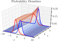
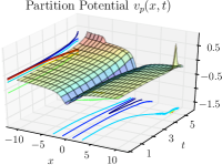
Figure 1: Left: Fragment densities at times $t=0$ and $t\approx T/4$ along with the total molecular density. Right: Exact partition potential $v_{p}\left(x,t\right)$. Parameters: $l=1$, $a=1$, $V_{0}=-1$, $E=0.1$, and $\omega=0.3$. A box of length 20 with 401 points was used.

The initial states of the fragments are obtained by solving the ground-state PDFT equations as prescribed in Ref. Mosquera and Wasserman (2013). This procedure generates the initial fragment Kohn-Sham orbitals needed to solve Eqs. 21. The distance between the wells was chosen to allow for a significant overlap between the initial fragments’ densities.

Even though the principle to construct $v_{p}({\bf r}t)$ is simple, note that Eq. (19) can also be written as $v_{p}=\mathcal{F}v_{p}$, where the operator $\mathcal{F}$ computes the right-hand-side of the equation, solves the differential equation, and finally outputs $v_{p}({\bf r}t)$. One could employ this formula recursively, i.e. $v_{p}^{k+1}=\mathcal{F}v_{p}^{k}$. We observed in our example that the term $\mathbf{Q}_{s\alpha}$ becomes noisy even after short times if the simulation box is discretized with large spatial steps. This noise is received by the partition potential during the propagation, and then it is received again by $\mathbf{Q}_{s,\alpha}$. This feedback process turns the algorithm unstable. The problem is reminiscent to what occurs in traditional TDDFT when one wants to find the exchange-correlation potential corresponding to a given density, even for only two electrons Lein and Kümmel (2005). To solve this problem in TDDFT, Ref. Nielsen et al. (2013) recently suggested an algorithm to control the feedback. They obtained encouraging results for a periodic system, but the methodology has not been tested for non-periodic systems.

Instead, we found the exact time-dependent partition potential by using the following optimization procedure: The density and current density of the total system are found at each time step using the Crank-Nicolson propagator. (Other propagation methods may also be used.) A guess is made for the partition potential at the next unknown time and the fragment wave functions are propagated forward in time using this guess. (For small time steps the value of the partition potential at the previous time step works well.) The fragment densities $\left(\left\{n_{\alpha}\right\},\,\left\{j_{\alpha}\right\}\right)$ are found using these fragment wave functions and added together to form an approximation to the total densities $\left(n,\,j\right)$. The errors $n_{\text{err}}=n-n_{\text{exact}}$ and $j_{\text{err}}=j-j_{\text{exact}}$ are computed and the residual $\text{norm}\left(n_{\text{err}}/n_{\text{exact}}\right)+\text{norm}\left(j_{\text{err}}/j_{\text{exact}}\right)$ is used in the L-BFGS-B optimizer Morales and Nocedal (2011), with the $L^{2}$ norm. The division by $n_{\text{exact}}$ and $j_{\text{exact}}$ weights the error in the asymptotic regions to help increase the convergence rate, similar to the weighting used in Peirs et al. (2003).

The right panel of Fig. (1) displays the resulting partition potential. The left panel shows the total density, along the corresponding fragment densities at the initial time and at 1/4^th of a period. The importance of memory effects Maitra and Burke (2001) is evident from Fig. (2), where the dashed-dotted lines labeled “Adiabatic” show the fragment densities obtained by solving the ground-state PDFT equations for the instantaneous $v({\bf r}t)$ at 1/4^th of a period. Clearly, the correct partition potential is needed. Only when the electric field strength is reduced by a factor of 10³ (keeping all other parameters fixed) does the adiabatic partition potential produce a molecular density that is visibly indistinguishable from the exact molecular density at time $t\approx T/4$. Interestingly, the approximation $v_{p}({\bf r}t)\approx v_{p}({\bf r}t_{0})$ (labeled “Static” in Fig. (2)) works qualitatively well for short times, certainly much better than the adiabatic approximation. The inset on the right panel of Fig. (2) shows how the static-$v_{p}$ approximation reproduces the correct dipole for short times.

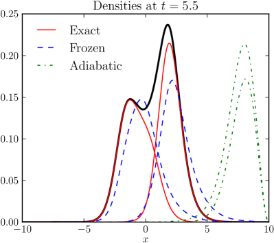
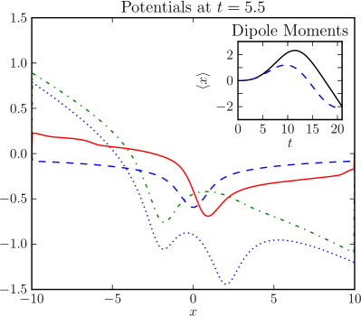
Figure 2: Left: Fragment densities at times $t\approx T/4$ along with the total molecular density (thick solid) calculated: with the exact $v_{p}(xt)$ (solid), static $v_{p}(xt)=v_{p}(xt_{0})$ (dashed), and adiabatic $v_{p}(xt)=v_{p}^{\rm PDFT}[n(xt)]$ (dash-dotted). Right: Corresponding partition potentials at $t\approx T/4$. Parameters: $l=1$, $a=1$, $V_{0}=-1$, $E=0.1$, and $\omega=0.3$. The inset compares the dipole moment obtained from the exact (solid) and static approximation to $v_{p}(xt)$ (dashed). The dotted line indicates the total (instantaneous) external potential.

In practice, successful application of our approach to large systems will ultimately rely on the quality of approximations to the time-dependent partition potential. The static approximation might be useful for short times. Furthermore, for problems whose physics is best described by invoking fragments (such as charge-transfer excitations), we believe that physically-meaningful approximations for $v_{p}({\bf r}t)$ will be simpler to construct than approximations for the highly non-local exchange-correlation potential and kernel of TDDFT. Work along these lines, as well as on the linear-response formalism, is ongoing.

Acknowledgements: We acknowledge support from the National Science Foundation CAREER program under grant No.CHE-1149968, and from the Office of Basic Energy Scieneces, U.S. Department of Energy, under grant No. DE-FG02-10ER16196.

References

- Runge and Gross (1984) E. Runge and E. K. U. Gross, Phys. Rev. Lett. 52, 997 (1984).
- Ullrich (2012) C. A. Ullrich, Time-dependent Density-functional Theory (Oxford University Press, USA, 2012).
- Burke et al. (2005) K. Burke, J. Werschnik, and E. K. U. Gross, J. Chem. Phys. 123, 062206 (2005).
- Yang (1991) W. Yang, Phys. Rev. Lett. 66, 1438 (1991).
- Severo Pereira Gomes and Jacob (2012) A. Severo Pereira Gomes and C. R. Jacob, Annu. Rep. Prog. Chem., Sect. C: Phys. Chem. 108, 222 (2012).
- Casida and Wesołowski (2004) M. E. Casida and T. A. Wesołowski, Int. J. Quantum Chem. 96, 577 (2004).
- Fradelos et al. (2011) G. Fradelos, J. J. Lutz, T. A. Wesołowski, P. Piecuch, and M. Włoch, J. Chem. Theory Comput. 7, 1647 (2011).
- Neugebauer et al. (2005) J. Neugebauer, M. J. Louwerse, E. J. Baerends, and T. A. Wesołowski, J. Chem. Phys. 122, 094115 (2005).
- Iozzi et al. (2004) M. F. Iozzi, B. Mennucci, J. Tomasi, and R. Cammi, J.Chem. Phys. 120, 7029 (2004).
- Hsu et al. (2001) C. P. Hsu, G. R. Fleming, M. Head-Gordon, and T. Head-Gordon, J. Chem. Phys. 114, 3065 (2001).
- Neugebauer (2010) J. Neugebauer, Phys. Rep. 489, 1 (2010).
- Neugebauer (2007) J. Neugebauer, J. Chem. Phys. 126, 134116 (2007).
- Yuen-Zhou et al. (2010) J. Yuen-Zhou, D. G. Tempel, C. A. Rodríguez-Rosario, and A. Aspuru-Guzik, Phys. Rev. Lett. 104, 043001 (2010).
- Elliott et al. (2010) P. Elliott, K. Burke, M. H. Cohen, and A. Wasserman, Phys. Rev. A 82, 024501 (2010).
- Cohen and Wasserman (2007) M. H. Cohen and A. Wasserman, J. Phys. Chem. A 111, 2229 (2007).
- Huang et al. (2011) C. Huang, M. Pavone, and E. A. Carter, J. Chem. Phys. 134, 154110 (2011).
- Cohen and Wasserman (2006) M. H. Cohen and A. Wasserman, J. Stat. Phys. 125, 1121 (2006).
- Pavanello (2013) M. Pavanello, (2013), arXiv:1212.4121 .
- Rajagopal (1996) A. K. Rajagopal, Phys. Rev. A 54, 3916 (1996).
- Vignale (2008) G. Vignale, Phys. Rev. A 77, 062511 (2008).
- Li and Tong (1985) T. C. Li and P. Q. Tong, Phys. Rev. A 31, 1950 (1985).
- Gross and Maitra (2012) E. K. U. Gross and N. T. Maitra (Springer Berlin / Heidelberg, Berlin, Heidelberg, 2012) Chap. 4, pp. 53–99.
- van Leeuwen (1999) R. van Leeuwen, Phys. Rev. Lett. 82, 3863 (1999).
- Mosquera and Wasserman (2013) M. A. Mosquera and A. Wasserman, Mol. Phys. 111, 505 (2013).
- Lein and Kümmel (2005) M. Lein and S. Kümmel, Phys. Rev. Lett. 94, 143003 (2005).
- Nielsen et al. (2013) S. E. B. Nielsen, M. Ruggenthaler, and R. van Leeuwen, Europhys. Lett. , 33001 (2013).
- Morales and Nocedal (2011) J. L. Morales and J. Nocedal, ACM Trans. Math. Softw. 38, 7:1 (2011).
- Peirs et al. (2003) K. Peirs, D. Van Neck, and M. Waroquier, Phys. Rev. A 67, 012505 (2003).
- Maitra and Burke (2001) N. T. Maitra and K. Burke, Phys. Rev. A 63, 042501 (2001).