Multiobjective Firefly Algorithm for Continuous Optimization

Abstract

Design problems in industrial engineering often involve a large number of design variables with multiple objectives, under complex nonlinear constraints. The algorithms for multiobjective problems can be significantly different from the methods for single objective optimization. To find the Pareto front and non-dominated set for a nonlinear multiobjective optimization problem may require significant computing effort, even for seemingly simple problems. Metaheuristic algorithms start to show their advantages in dealing with multiobjective optimization. In this paper, we extend the recently developed firefly algorithm to solve multiobjective optimization problems. We validate the proposed approach using a selected subset of test functions and then apply it to solve design optimization benchmarks. We will discuss our results and provide topics for further research.

Keywords: algorithm, firefly algorithm, metaheuristic, multiobjective, engineering design, global optimization.

Citation details: X. S. Yang, Multiobjective firefly algorithm for continuous optimization, Engineering with Computers, Vol. 29, Issue 2, pp. 175–184 (2013).

Revised manuscript: Ms. No. EWCO-D-11-00145 (Engineering with Computers)

1 Introduction

Design optimization in engineering and industry often concerns multiple design objectives under complex, highly nonlinear constraints. Different objectives often conflict each other, and sometimes, truly optimal solutions do not exist, and some compromises and approximations are often needed [1, 2, 3]. Further to this complexity, a design problem is subjected to various design constraints, limited by design codes or standards, material properties and the optimal utility of available resources and costs [2, 4]. Even for global optimization problems with a single objective, if the design functions are highly nonlinear, global optimality is not easy to reach. Metaheuristic algorithms are very powerful in dealing with this kind of optimization, and there are many review articles and textbooks [5, 6, 7, 8, 9, 10, 11].

In contrast with single objective optimization, multiobjective problems are much more difficult and complex [5, 12]. Firstly, no single unique solution is the best; instead, a set of non-dominated solutions should be found in order to get a good approximation to the true Pareto front. Secondly, even if an algorithm can find solution points on the Pareto front, there is no guarantee that multiple Pareto points will distribute along the front uniformly, often they do not. Thirdly, algorithms which work well for single objective optimization usually cannot directly work for multiobjective problems, unless under special circumstances such as combining multiobjectives into a single objective using some weighted sum method. Substantial modifications are needed to make algorithms for single objective optimization work. In addition to these difficulties, a further challenge is how to generate solutions with enough diversity so that new solutions can sample the search space efficiently.

Furthermore, real-world optimization problems always involve some degree of uncertainty or noise. For example, materials properties for a design product may vary significantly. An optimal design should be robust enough to allow such inhomogeneity, which provides a set of multiple feasible solution sets. Consequently, optimal solutions among the robust Pareto set can provide good options so that decision-makers or designers can choose to suit their needs. Despite these challenges, multiobjective optimization has many powerful algorithms with many successful applications [6, 13, 14, 15, 43]. In addition, metaheuristic algorithms start to emerge as a major player for multiobjective global optimization, they often mimic the successful characteristics in Nature, especially biological systems [9, 10], while some algorithms are inspired by the beauty of music [16]. Many new algorithms are emerging with many important applications [8, 10, 13, 17, 18, 19, 20].

For example, multiobjective genetic algorithms are widely known [15, 21], while multiobjective differential evolution algorithms are also very powerful [22, 23]. In addition, multiobjective particle swarm optimizers are becoming increasingly popular [19]. As there are many algorithms, one of our motivations in the present study is to compare the performance of these algorithms for real-world application.

Most metaheuristic algorithms are based on the so-called swarm intelligence. PSO is a good example, it mimics some characteristics of birds and fish swarms. Recently, a new metaheuristic search algorithm, called Firefly Algorithm (FA), has been developed by Yang [9, 11]. FA mimics some characteristics of tropic firefly swarms and their flashing behaviour [10, 11]. A firefly tends to be attracted towards other fireflies with higher flash intensity. This algorithm is thus different from PSO and can have two advantages: local attractions and automatic regrouping. As light intensity decreases with distance, the attraction among fireflies can be local or global, depending on the absorbing coefficient, and thus all local modes as well as global modes will be visited. In addition, fireflies can also subdivide and thus regroup into a few subgroups due to neighboring attraction is stronger than long-distance attraction, thus it can be expected each subgroup will swarm around a local mode. This latter advantage makes it particularly suitable for multimodal global optimization problems [10, 11].

Preliminary studies show that it is very promising and could outperform existing algorithms such as particle swarm optimization (PSO). For example, a Firefly-LGB algorithm, based on firefly algorithm and Linde-Buzo-Gray (LGB) algorithms for vector quantization of digital image compression, was developed by Horng and Jiang [24], and their results suggested that Firefly-LGB is faster than other algorithms such as particle swarm optimization LBG (PSO-LBG) and honey-bee mating optimization LBG (HBMO-LBG). Apostolopoulos and Vlachos provided a detailed background and analysis over a wide range of test problems [25], and they also solved multiobjective load dispatch problem using a weighted sum method by combining multiobjectives into a single objective, and their results are very promising. The preliminary successful results of firefly-based algorithms provide another motivation for this paper. That is to see how this algorithm can be extended to solve multiobjective optimization problems.

In this paper, we will extend FA to solve multiobjective problems and formulate a multiobjective firefly algorithm (MOFA). We will first validate it against a subset of multiobjective test functions. Then, we will apply it to solve design optimisation problems in engineering, including bi-objective beam design and a design of a disc brake. Finally, we will discuss the unique features of the proposed algorithm as well as topics for further studies.

2 Multiobjective Firefly Algorithm

In order to extend the firefly algorithm for single objective optimization to solve multiobjective problems, let us briefly review its basic version.

2.1 The Basic Firefly Algorithm

Firefly Algorithm was developed by Yang for continuous optimization [9, 10, 27], which was subsequently applied into structural optimization [26] and image processing [24]. FA was based on the flashing patterns and behaviour of fireflies. In essence, FA uses the following three idealized rules: (1) Fireflies are unisex so that one firefly will be attracted to other fireflies regardless of their sex; (2) The attractiveness of a firefly is proportional to its brightness and they both decrease with distance. Thus for any two flashing fireflies, the less brighter one will move towards the brighter one. If there is no brighter one than a particular firefly, it will move randomly; (3) The brightness of a firefly is determined by the landscape of the objective function.

For a maximization problem, the brightness can simply be proportional to the value of the objective function. As both light intensity and attractiveness affect the movement of fireflies in the firefly algorithm, we have to define their variations. For simplicity, we can always assume that the attractiveness of a firefly is determined by its brightness which in turn is associated with the encoded objective function. In the simplest case for maximum optimization problems, the brightness $I$ of a firefly at a particular location $x$ can be chosen as $I({\mbox{\boldmath$x$}})\propto f({\mbox{\boldmath$x$}})$.

However, the attractiveness $\beta$ is relative, it should be seen in the eyes of the beholder or judged by the other fireflies. Thus, it will vary with the distance $r_{ij}$ between firefly $i$ and firefly $j$. Therefore, we can now define the attractiveness $\beta$ of a firefly by

$$\beta=\beta_{0}e^{-\gamma r^{2}},$$ (1)

where $\beta_{0}$ is the attractiveness at $r=0$. In fact, equation (1) defines a characteristic distance $\Gamma=1/\sqrt{\gamma}$ over which the attractiveness changes significantly from $\beta_{0}$ to $\beta_{0}e^{-1}$. The distance between any two fireflies $i$ and $j$ at ${\mbox{\boldmath$x$}}_{i}$ and ${\mbox{\boldmath$x$}}_{j}$, respectively, is the Cartesian distance $r_{ij}=||{\mbox{\boldmath$x$}}_{i}-{\mbox{\boldmath$x$}}_{j}||$. It is worth pointing out that the distance $r$ defined above is not limited to the Euclidean distance. In fact, any measure that can effectively characterize the quantities of interest in the optimization problem can be used as the ‘distance’ $r$. We can define other distance $r$ in the $n$-dimensional hyperspace, depending on the type of problem of our interest.

For any given two fireflies ${\mbox{\boldmath$x$}}_{i}$ and ${\mbox{\boldmath$x$}}_{j}$, the movement of firefly $i$ is attracted to another more attractive (brighter) firefly $j$ is determined by

$${\mbox{\boldmath$x$}}_{i}^{t+1}={\mbox{\boldmath$x$}}_{i}^{t}+\beta_{0}e^{-\gamma r^{2}_{ij}}({\mbox{\boldmath$x$}}_{j}^{t}-{\mbox{\boldmath$x$}}_{i}^{t})+\alpha_{t}\;{\mbox{\boldmath$\epsilon$}}_{i}^{t},$$ (2)

where the second term is due to the attraction. The third term is randomization with $\alpha_{t}$ being the randomization parameter, and ${\mbox{\boldmath$\epsilon$}}_{i}^{t}$ is a vector of random numbers drawn from a Gaussian distribution or uniform distribution. The location of fireflies can be updated sequentially, by comparing and updating each pair of them in every iteration cycle.

For most implementations, we can take $\beta_{0}=1$ and $\alpha_{t}=O(1)$, though we found that it is better to use a time-dependent $\alpha_{t}$ so that randomness can be reduced gradually as iterations proceed. It is worth pointing out that (2) is a random walk biased towards the brighter fireflies. If $\beta_{0}=0$, it becomes a simple random walk. Furthermore, the randomization term can easily be extended to other distributions such as Lévy flights [28].

The parameter $\gamma$ now characterizes the variation of the attractiveness, and its value is crucially important in determining the speed of the convergence and how the FA algorithm behaves. In theory, $\gamma\in[0,\infty)$, but in practice, $\gamma=O(1)$ is determined by the characteristic distance $\Gamma$ of the system to be optimized. Thus, for most applications, it typically varies from $10^{-5}$ to $10^{5}$.

To consider the scale variations of each problem, we now use rescaled, vectorized parameters

$$\alpha=0.01L,\quad\gamma=0.5/L^{2},$$ (3)

with $L=(U_{b}-L_{b})$ where $U_{b}$ and $L_{b}$ are the upper and lower bounds of $x$, respectively. Here the factor $0.01$ is to make sure the random walks is not too aggressive, and this value has been obtained by a parametric study.

2.2 Multiobjective Firefly Algorithm

For multiobjective optimization, one way is to combine all objectives into a single objective so that algorithms for single objective optimization can be used without much modifications. For example, FA can be used directly to solve multiobjective problems in this manner, and a detailed study was carried out by Apostolopoulos and Vlachos [25].

Another way is to extend the firefly algorithm to produce Pareto optimal front directly. By extending the basic ideas of FA, we can develop the following Multi-objective Firefly Algorithm (MOFA), which can be summarized as the pseudo code listed in Fig. 1.

   Define objective functions $f_{1}({\mbox{\boldmath$x$}}),...,f_{K}({\mbox{\boldmath$x$}})$ where ${\mbox{\boldmath$x$}}=(x_{1},...,x_{d})^{T}$

Initialize a population of $n$ fireflies ${\mbox{\boldmath$x$}}_{i}\;(i=1,2,...,n)$
 while ($t<$MaxGeneration)
  for $i,j=1:n$ (all $n$ fireflies)
   Evaluate their approximations $PF_{i}$ and $PF_{j}$ to the Pareto front
      if $i\neq j$ and when all the constraints are satisfied
   if $PF_{j}$ dominates $PF_{i}$,
    Move firefly $i$ towards $j$ using (2)
    Generate new ones if the moves do not satisfy all the constraints
   end if
   if no non-dominated solutions can be found
    Generate random weights $w_{k}$ ($k=1,...,K$)
    Find the best solution ${\mbox{\boldmath$g$}}_{*}^{t}$ (among all fireflies) to minimize $\psi$ in (4)
    Random walk around ${\mbox{\boldmath$g$}}_{*}^{t}$ using (5)
   end if
   Update and pass the non-dominated solutions to next iterations
  end
  Sort and find the current best approximation to the Pareto front
  Update $t\leftarrow t+1$
 end while
 Postprocess results and visualisation;  

Figure 1: Pseudo Code: Multiobjective firefly algorithm (MOFA).

The procedure starts with an appropriate definition of objective functions with associated nonlinear constraints. We first initialize a population of $n$ fireflies so that they should distribute among the search space as uniformly as possible. This can be achieved by using sampling techniques via uniform distributions. Once the tolerance or a fixed number of iterations is defined, the iterations start with the evaluation of brightness or objective values of all the fireflies and compare each pair of fireflies. Then, a random weight vector is generated (with the sum equal to 1), so that a combined best solution ${\mbox{\boldmath$g$}}_{*}^{t}$ can be obtained. The non-dominated solutions are then passed onto the next iteration. At the end of a fixed number of iterations, in general $n$ non-dominated solution points can be obtained to approximate the true Pareto front.

In order to do random walks more efficiently, we can find the current best ${\mbox{\boldmath$g$}}_{*}^{t}$ which minimizes a combined objective via the weighted sum

$$\psi({\mbox{\boldmath$x$}})=\sum_{k=1}^{K}w_{k}f_{k},\quad\sum_{k=1}^{K}w_{k}=1.$$ (4)

Here $w_{k}=p_{k}/K$ where $p_{k}$ are the random numbers drawn from a uniform distributed Unif[0,1]. In order to ensure that $\sum_{k}w_{k}=1$, a rescaling operation is performed after generating $K$ uniformly distributed numbers. It is worth pointing out that the weights $w_{k}$ should be chosen randomly at each iteration, so that the non-dominated solution can sample diversely along the Pareto front.

If a firefly is not dominated by others in the sense of Pareto front, the firefly moves

$${\mbox{\boldmath$x$}}_{i}^{t+1}={\mbox{\boldmath$g$}}_{*}^{t}+\alpha_{t}\;{\mbox{\boldmath$\epsilon$}}_{i}^{t},$$ (5)

where ${\mbox{\boldmath$g$}}_{*}^{t}$ is the best solution found so far for a given set of random weights.

Furthermore, the randomness can be reduced as the iterations proceed, and this can be achieved in a similar manner as that for simulated annealing and other random reduction techniques [11]. We will use

$$\alpha_{t}=\alpha_{0}0.9^{t},$$ (6)

where $\alpha_{0}$ is the initial randomness factor.

2.3 Pareto Optimal Front

For a minimization problem, a solution vector ${\mbox{\boldmath$u$}}=(u_{1},..,u_{n})^{T}$ is said to dominate another vector ${\mbox{\boldmath$v$}}=(v_{1},...,v_{n})^{T}$ if and only if $u_{i}\leq v_{i}$ for $\forall i\in\{1,...,n\}$ and $\exists i\in\{1,...,n\}:u_{i}<v_{i}.$ In other words, no component of $u$ is larger than the corresponding component of $v$, and at least one component is smaller. Similarly, we can define another dominance relationship $\preceq$ by

$${\mbox{\boldmath$u$}}\preceq{\mbox{\boldmath$v$}}\Longleftrightarrow{\mbox{\boldmath$u$}}\prec{\mbox{\boldmath$v$}}\vee{\mbox{\boldmath$u$}}={\mbox{\boldmath$v$}}.$$ (7)

It is worth pointing out that for maximization problems, the dominance can be defined by replacing $\prec$ with $\succ$. Therefore, a point ${\mbox{\boldmath$x$}}_{*}$ is called a non-dominated solution if no solution can be found that dominates it [5].

The Pareto front $PF$ of a multiobjective can be defined as the set of non-dominated solutions so that

$$PF=\{{\mbox{\boldmath$s$}}\in{\cal S}\Big{|}\exists/\;{\mbox{\boldmath$s^{\prime}$}}\in{\cal S}:{\mbox{\boldmath$s^{\prime}$}}\prec{\mbox{\boldmath$s$}}\},$$ (8)

where ${\cal S}$ is the solution set.

To obtain a good approximation of the Pareto front, a diverse range of solutions should be generated using efficient techniques [15, 29, 30, 31]. For example, Lévy flights ensure the good diversity of the solutions, as we can see from later simulations.

3 Numerical Results

We have implemented the proposed MOFA in Matlab, and we have first validated it against a set of multiobjective test functions. Then, we have used it to solve some industrial design of structures. In order to obtain the right algorithm-dependent parameters, we have carried out detailed parametric studies.

3.1 Parametric Studies

By varying the parameters $\alpha_{0}$, $\beta_{0}$ and $\gamma$, we have carried out parametric studies by setting $\alpha_{0}=0$ to $1$ with a step of $0.05$, $\beta_{0}=0$ to $1$ with a step of $0.05$, and $\gamma=0.1$ to $10$ with a step of $0.1$ and then $1$. From simulations, we found that we can use $\alpha_{0}=0.1$ to $0.5$, $\beta_{0}=0.7$ to $1.0$ and $\gamma=1$ for most problems.

The stopping criterion can be defined in many ways. We can either use a given tolerance or a fixed number of iterations. For a given tolerance, we should have some prior knowledge of the true optimum of the objective function so that we can calculate the differences between the current best solutions and the true optimal solution so that we can assess if the tolerance is met. In reality, we usually do not know the true optimum in advance, except for a few well-tested cases. In addition, the number of functions can vary significantly from function to function even for the same tolerance. From the implementation point of view, a fixed number of iterations is not only easy to implement, but also suitable to compare the closeness of Pareto front of different functions. So we have set the fixed number iterations as 2500, which is sufficient for most problems. If necessary, we can also increase it to a larger number.

One can generate points of the Pareto front in two ways: increase the population size $n$ or run the program a few more times. Through simulations, we found that increasing $n$ typically leads to a longer computing time than re-running the program a few times. This may be due to the fact that manipulations of large matrices or longer vectors usually take longer. In order to generate $M$ points using a smaller population size $n$, it requires to run the program $M/n$ times, each run with different, random initial configurations but with the same number of iterations $t=2500$. For example, to generate $M=200$ points, we can use $n=50$, which is easily done within a few minutes. Therefore, in all our simulations, we will use the fixed parameters: $n=50$, $\alpha_{0}=0.25$, $\beta_{0}=1$ and $\gamma=1$.

3.2 Multiobjective Test Functions

There are many different test functions for multiobjective optimization [32, 33, 34], but a subset of a few widely used functions provides a wide range of diverse properties in terms of Pareto front and Pareto optimal set. To validate the proposed MOFA, we have selected a subset of these functions with convex, non-convex and discontinuous Pareto fronts. We also include functions with more complex Pareto sets. To be more specific in this paper, we have tested the following 5 functions:

• Schaffer’s Min-Min (SCH) test function with convex Pareto front [21, 35]

  $$f_{1}(x)=x^{2},\quad f_{2}(x)=(x-2)^{2},\quad-10^{3}\leq x\leq 10^{3}.$$ (9)

• ZDT1 function with a convex front [33, 34]

  $$f_{1}(x)=x_{1},\quad f_{2}(x)=g(1-\sqrt{f_{1}/g}),$$

  $$g=1+\frac{9\sum_{i=2}^{d}x_{i}}{d-1},\quad x_{i}\in[0,1],\;i=1,...,30,$$ (10)

  where $d$ is the number of dimensions. The Pareto optimality is reached when $g=1$, and thus the true Pareto front is $f_{2}=1-\sqrt{f_{1}}$.

• ZDT2 function with a non-convex front

  $$f_{1}(x)=x_{1},\quad f_{2}(x)=g(1-\frac{f_{1}}{g})^{2},$$

• ZDT3 function with a discontinuous front

  $$f_{1}(x)=x_{1},\quad f_{2}(x)=g\Big{[}1-\sqrt{\frac{f_{1}}{g}}-\frac{f_{1}}{g}\sin(10\pi f_{1})\Big{]},$$

  where $g$ in functions ZDT2 and ZDT3 is the same as in function ZDT1. In the ZDT3 function, $f_{1}$ varies from $0$ to $0.852$ and $f_{2}$ from $-0.773$ to $1$.

• LZ function [20, 36]

  $$f_{1}=x_{1}+\frac{2}{|J_{1}|}\sum_{j\in J_{1}}\Big{[}x_{j}-\sin(6\pi x_{1}+\frac{j\pi}{d})\Big{]}^{2},$$

  $$f_{2}=1-\sqrt{x_{1}}++\frac{2}{|J_{2}|}\sum_{j\in J_{2}}\Big{[}x_{j}-\sin(6\pi x_{1}+\frac{j\pi}{d})\Big{]}^{2},$$ (11)

  where $J_{1}=\{j|j$ is odd $\}$ and $J_{2}=\{j|j$ is even $\}$ where $2\leq j\leq d$. This function has a Pareto front $f_{2}=1-\sqrt{f_{1}}$ with a Pareto set

  $$x_{j}=\sin(6\pi x_{1}+\frac{j\pi}{d}),\quad j=2,3,...,d,\quad x_{1}\in[0,1].$$ (12)

After generating 200 Pareto points by MOFA, these points are compared with the true front $f_{2}=1-\sqrt{f_{1}}$ of ZDT1 (see Fig. 2).

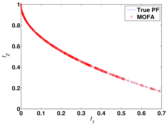
Figure 2: Pareto front of ZDT1: a comparison of the front found by MOFA and the true Pareto front (true PF). Here the horizontal axis is $f_{1}$ while the vertical axis is $f_{2}$.

Let us define the distance or error between the estimated Pareto front $PF^{e}$ to its corresponding true front $PF^{t}$ as

$$E_{f}=||PF^{e}-PF^{t}||^{2}=\sum_{j=1}^{N}(PF_{j}^{e}-PF_{j}^{t})^{2},$$ (13)

where $N$ is the number of points. For all the test functions, the true Pareto fronts have analytical forms [20, 33, 35], for example, $f_{2}=1-\sqrt{f_{1}}$ for ZDT1, which makes the above calculations straightforward.

The convergence property can be viewed by following the iterations. As this measure is an absolute measure, which depends on the number of points. Sometimes, it is easier to use relative measure using generalized distance

$$D_{g}=\frac{1}{N}\sqrt{\sum_{j=1}^{N}(PF_{j}-PF_{j}^{t})^{2}}.$$ (14)

Fig. 3 shows the exponential-like decrease of $D_{g}$ as the iterations proceed. We can see clearly that our MOFA algorithm indeed converges almost exponentially. The results for all the functions are summarized in Table 1, and the estimated Pareto fronts and true fronts of other functions are shown in Fig. 4 and Fig. 5. In all these figures, the vertical axis is $f_{2}$ and the horizontal axis is $f_{1}$.

3.3 Comparison Study

In order to compare the performance of the proposed MOFA with other established multiobjective algorithms, we have carefully selected a few algorithms with available results from the literature. When the results have not been available, we have implemented the algorithms using well-documented studies and then generated new results using these algorithms. In particular, we have used other methods for comparison, including vector evaluated genetic algorithm (VEGA) [21], NSGA-II [37], multiobjective differential evolution (MODE) [23, 38], differential evolution for multiobjective optimization (DEMO) [22], multiobjective bees algorithms (Bees) [39], and strength Pareto evolutionary algorithm (SPEA) [37, 40]. The performance measures in terms of generalized distance $D_{g}$ are summarized in Table 2 for all the above major methods.

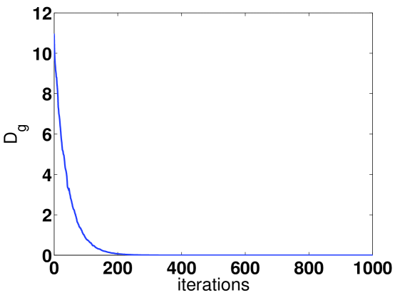
Figure 3: Convergence of the proposed MOFA. The least-square distance (vertical axis) from the estimated front to the true front of ZDT1 for the first 1000 iterations.

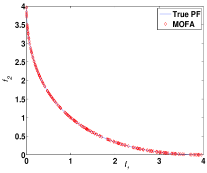
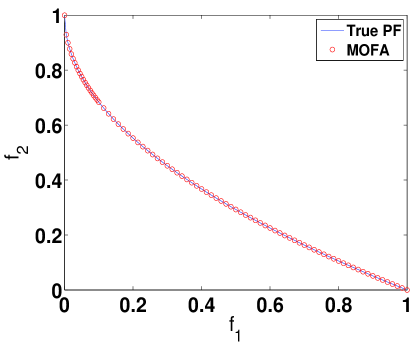
Figure 4: a) Pareto front of test function SCH, and b) Pareto front of test function ZDT2.

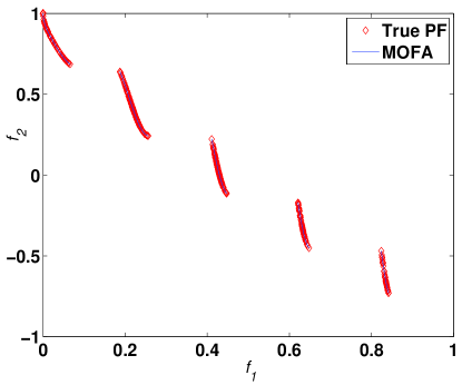
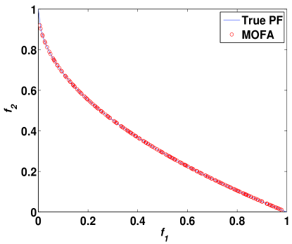
Figure 5: a) Pareto front of test function ZDT2, and b) Pareto front of test function LZ.

Table 1: Summary of results.

Functions	Errors (1000 iterations)	Errors (2500 iterations)
SCH	5.5E-09	4.0E-22
ZDT1	2.3E-6	5.4E-19
ZDT2	8.9E-6	1.7E-14
ZDT3	3.7E-5	2.5E-11
LZ	2.0E-6	7.7E-12

It is clearly seen from Table 2 that the proposed MOFA obtained better results for almost all five cases, though for ZDT2 function our result is the same order (still slightly better) as that by DEMO.

Table 2: Comparison of $D_{g}$ for $n=50$ and $t=500$ iterations.

Methods	ZDT1	ZDT2	ZDT3	SCH	LZ
VEGA	3.79E-02	2.37E-03	3.29E-01	6.98E-02	1.47E-03
NSGA-II	3.33E-02	7.24E-02	1.14E-01	5.73E-03	2.77E-02
MODE	5.80E-03	5.50E-03	2.15E-02	9.32E-04	3.19E-03
DEMO	1.08E-03	7.55E-04	1.18E-03	1.79E-04	1.40E-03
Bees	2.40E-02	1.69E-02	1.91E-01	1.25E-02	1.88E-02
SPEA	1.78E-03	1.34E-03	4.75E-02	5.17E-03	1.92E-03
MOFA	1.90E-04	1.52E-04	1.97E-04	4.55E-06	8.70E-04

4 Design Optimization

Design optimization, especially design of structures, has many applications in engineering and industry. As a result, there are many different benchmarks with detailed studies in the literature [39, 41, 42]. Some benchmarks have been solved by various methods, while others do not have all available data for comparison. Thus, we have chosen the welded beam design, and disc brake design among the well-known benchmarks [42, 43, 44]. In the rest of this paper, we will solve these two design benchmarks using MOFA.

4.1 Welded Beam Design

Multiobjective design of a welded beam is a classical benchmark which has been solved by many researchers [6, 12, 44]. The problem has four design variables: the width $w$ and length $L$ of the welded area, the depth $d$ and thickness $h$ of the main beam. The objective is to minimize both the overall fabrication cost and the end deflection $\delta$.

The detailed formulation can be found in [6, 12, 44]. Here we only rewrite the main problem as

$$\textrm{minimise }\;f_{1}({\mbox{\boldmath$x$}})=1.10471w^{2}L+0.04811dh(14.0+L),\;\textrm{ minimize }\;f_{2}=\delta,$$ (15)

subject to

$$\begin{array}[]{lll}g_{1}({\mbox{\boldmath$x$}})=w-h\leq 0,\vspace{2pt}\\ \vspace{3pt}g_{2}({\mbox{\boldmath$x$}})=\delta({\mbox{\boldmath$x$}})-0.25\leq 0,\\ \vspace{3pt}g_{3}({\mbox{\boldmath$x$}})=\tau({\mbox{\boldmath$x$}})-13,600\leq 0,\\ \vspace{3pt}g_{4}({\mbox{\boldmath$x$}})=\sigma({\mbox{\boldmath$x$}})-30,000\leq 0,\\ \vspace{3pt}g_{5}({\mbox{\boldmath$x$}})=0.10471w^{2}+0.04811hd(14+L)-5.0\leq 0,\\ \vspace{3pt}g_{6}({\mbox{\boldmath$x$}})=0.125-w\leq 0,\\ \vspace{3pt}g_{7}({\mbox{\boldmath$x$}})=6000-P({\mbox{\boldmath$x$}})\leq 0,\end{array}$$ (16)

where

$$\begin{array}[]{ll}\sigma({\mbox{\boldmath$x$}})=\frac{504,000}{hd^{2}},&Q=6000(14+\frac{L}{2}),\\ \\ D=\frac{1}{2}\sqrt{L^{2}+(w+d)^{2}},&J=\sqrt{2}\;wL[\frac{L^{2}}{6}+\frac{(w+d)^{2}}{2}],\\ \\ \delta=\frac{65,856}{30,000hd^{3}},&\beta=\frac{QD}{J},\\ \\ \alpha=\frac{6000}{\sqrt{2}wL},&\tau({\mbox{\boldmath$x$}})=\sqrt{\alpha^{2}+\frac{\alpha\beta L}{D}+\beta^{2}},\\ \\ P=0.61423\times 10^{6}\;\frac{dh^{3}}{6}(1-\frac{d\sqrt{30/48}}{28}).&\end{array}$$ (17)

The simple limits or bounds are $0.1\leq L,d\leq 10$ and $0.125\leq w,h\leq 2.0$.

By using the MOFA, we have solved this design problem. The approximate Pareto front generated by the 50 non-dominated solutions after 1000 iterations are shown in Fig. 6. This is consistent with the results obtained by others [39, 44]. In addition, our results are more smooth with fewer iterations, which shows the efficiency of the proposed MOFA. A comparison of the results with those obtained by other methods is shown in Fig. 7 where we can see MOFA converged faster.

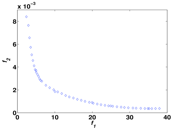
Figure 6: Pareto front for the bi-objective beam design where the horizontal axis corresponds to cost and the vertical axis corresponds to deflection.

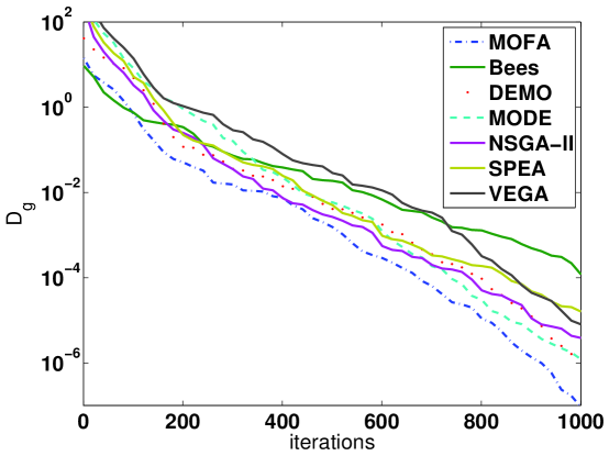
Figure 7: Convergence comparison for the beam design.

4.2 Design of a Disc Brake

Design of a multiple disc brake is another benchmark for multiobjective optimization [12, 18, 44]. The objectives are to minimize the overall mass and the braking time by choosing optimal design variables: the inner radius $r$, outer radius $R$ of the discs, the engaging force $F$ and the number of the friction surfaces $s$. This is under the design constraints such as the torque, pressure, temperature, and length of the brake. This bi-objective design problem can be written as:

$$\textrm{Minimize }\;f_{1}({\mbox{\boldmath$x$}})=4.9\times 10^{-5}(R^{2}-r^{2})(s-1),\quad f_{2}({\mbox{\boldmath$x$}})=\frac{9.82\times 10^{6}(R^{2}-r^{2})}{Fs(R^{3}-r^{3})},$$ (18)

subject to

$$\begin{array}[]{lll}g_{1}({\mbox{\boldmath$x$}})=20-(R-r)\leq 0,\\ \vspace{5pt}g_{2}({\mbox{\boldmath$x$}})=2.5(s+1)-30\leq 0,\\ \vspace{5pt}g_{3}({\mbox{\boldmath$x$}})=\frac{F}{3.14(R^{2}-r^{2})}-0.4\leq 0,\\ \vspace{5pt}g_{4}({\mbox{\boldmath$x$}})=\frac{2.22\times 10^{-3}F(R^{3}-r^{3})}{(R^{2}-r^{2})^{2}}-1\leq 0,\\ \vspace{5pt}g_{5}({\mbox{\boldmath$x$}})=900-\frac{0.0266Fs(R^{3}-r^{3})}{(R^{2}-r^{2})}\leq 0.\end{array}$$ (19)

The simple limits are

$$55\leq r\leq 80,\;75\leq R\leq 110,\;1000\leq F\leq 3000,\;2\leq s\leq 20.$$ (20)

The detail formulation of this problem and background descriptions can be found in [41, 12, 18, 44]. The Pareto front of 50 solution points after 1000 iterations obtained by MOFA is shown in Fig. 8, where we can see that the results are smooth and are the same or better than the results obtained in [44]. This can also be seen from the comparison of converge rates shown in Fig. 9.

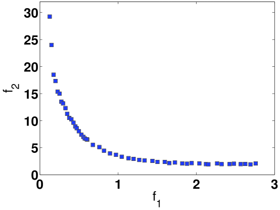
Figure 8: Pareto front for the disc brake design where $f_{2}$ is the vertical axis and $f_{1}$ is the horizontal axis.

In order to see how the proposed MOFA performs for the real-world design problems, we also solved the same problems using other available multiobjective algorithms. The comparison of the convergence rates is plotted in the logarithmic scales in Fig. 7 and Fig. 9. We can see from these two figures that the convergence rates of MOFA are of the highest in an exponentially decreasing way in both cases. This again suggests that MOFA provides better solutions in a more efficient way.

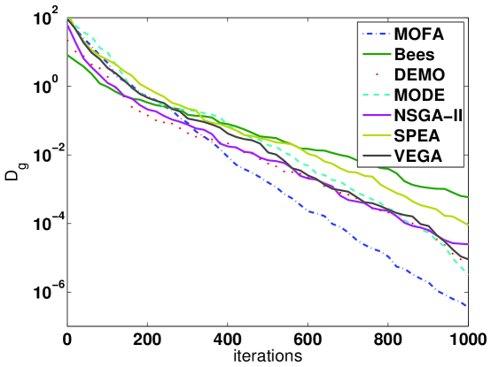
Figure 9: Convergence comparison for the disc brake design.

The simulations for these benchmarks and test functions suggest that MOFA is a very efficient algorithm for multiobjective optimization. It can deal with highly nonlinear problems with complex constraints and diverse Pareto optimal sets.

5 Conclusions

Multiobjective optimization problems are typically very difficult to solve. We have successfully formulated a new algorithm for multiobjective optimization, namely, multiobjective firefly algorithm (MOFA), based on the recently developed firefly algorithm. The proposed MOFA has been tested against a subset of well-chosen test functions, and then been applied to solve design optimization benchmarks in industrial engineering.

By comparing with other algorithms, the present results suggest that MOFA is an efficient multiobjective optimizer. Further studies can focus on parametric studies which can be very useful to identify the optimal ranges of parameters for various optimization problems.

In addition, convergence analysis of MOFA will also show insight in the working mechanism of the algorithm, and this may also help to improve the proposed algorithm or even design new algorithms. For example, hybridization with other algorithms may also prove to be fruitful. Furthermore, formulation of a discrete MOFA will also be an important topic for further research.

References

- [1] Cagnina L. C., Esquivel S. C., and Coello C. A., (2008). Solving engineering optimization problems with the simple constrained particle swarm optimizer, Informatica, 32, 319-326.
- [2] Deb K., (2001). Multi-Objective Optimization Using Evolutionary Algorithms, John Wiley and Sons, New York.
- [3] Leifsson L. and Koziel S. (2010), Multi-fidelity design optimization of transonic airfoils using physics-based surrogate modeling and shape-preserving response prediction, J. Comp. Science, 1, 98-106.
- [4] Farina M., Deb K. and Amota P., (2004). Dynamic multiobjective optimization problems: test cases, approximations, and applications, IEEE Trans. Evol. Comp., 8, 425-442.
- [5] Coello C. A. C., (1999). An updated survey of evolutionary multiobjective optimization techniques: state of the art and future trends, in: Proc. of 1999 Congress on Evolutionary Computation, CEC99, DOI 10.1109/CEC.1999.781901
- [6] Deb K., (1999). Evolutionary algorithms for multi-criterion optimization in engieering design, in: Evolutionary Aglorithms in Engineering and Computer Science, Wiley, pp. 135-161.
- [7] Geem Z. W., Music-Inspired Harmony Search Algorithm: Theory and Applications, Springer, (2009).
- [8] Talbi E.-G., (2009). Metaheuristics: From Design to Implementation, John Wiley and Sons, 624 pp.
- [9] Yang X. S., (2008). Nature-Inspired Metaheuristic Algorithms, Luniver Press.
- [10] Yang X. S., (2010). Engineering Optimisation: An Introduction with Metaheuristic Applications, John Wiley and Sons.
- [11] Yang X. S., (2009). Firefly algorithms for multimodal optimization, in: Stochastic Algorithms: Foundations and Applications, SAGA 2009, LNCS 5792, 169-178.
- [12] Gong W. Y., Cai Z. H., Zhu L., An effective multiobjective differential evolution algorithm for engineering design, Struct. Multidisc. Optimization, 38, 137-157 (2009).
- [13] Abbass H. A. and Sarker R., (2002). The Pareto diffential evolution algorithm, Int. J. Artificial Intelligence Tools, 11(4), 531-552 (2002).
- [14] Banks A., Vincent J. and Anyakoha C., (2008). A review of particle swarm optimization. Part II: hydridisation, combinatorial, multicriteria and constrained optimization, and indicative applications, Natural Computing, 109-124 (2008).
- [15] Konak A., Coit D. W. and Smith A. E., (2006). Multiobjective optimization using genetic algorithms: a tutorial, Reliability Engineering and System Safety, 91, 992-1007.
- [16] Geem Z. W., Kim J. H. and Loganathan G. V., A New Heuristic Optimization Algorithm: Harmony Search, Simulation, 76, 60-68 (2001).
- [17] Kennedy J. and Eberhart R. C., (1995). Particle swarm optimization, in: Proc. of IEEE International Conference on Neural Networks, Piscataway, NJ., 1942-1948.
- [18] Osyczka A. and Kundu S., (1995). A genetic algorithm-based multicriteria optimization method, Proc. 1st World Congr. Struct. Multidisc. Optim., 909-914.
- [19] Reyes-Sierra M. and Coello C. A. C., (2006). Multi-objective particle swarm optimizers: A survey of the state-of-the-art, Int. J. Comput. Intelligence Res., 2(3), 287-308.
- [20] Zhang Q. F. and Li H., (2007). MOEA/D: a multiobjective evolutionary algorithm based on decomposition, IEEE Trans. Evol. Comput., 11, 712-731.
- [21] Schaffer J.D., (1985). Multiple objective optimization with vector evaluated genetic algorithms, in: Proc. 1st Int. Conf. Genetic Aglorithms, pp. 93-100.
- [22] Robič T. and Filipič B., (2005). DEMO: differential evolution for multiobjective optimization, in: EMO 2005 (eds. C. A. Coello Coello et al.), LNCS 3410, 520-533.
- [23] Xue F., Multi-objective differential evolution: theory and applications, PhD thesis, Rensselaer Polytechnic Institute, (2004).
- [24] Horng M.-H. and Jiang T. W., (2010). The codebook design of image vector quantization based on the firefly algorithm, in: Computational Collective Intelligence, Technologies and Applications, LNCS, 6423, pp. 438-447.
- [25] Apostolopoulos T. and Vlachos A., (2011). Application of the Firefly Algorithm for Solving the Economic Emissions Load Dispatch Problem, Int. Journal of Combinatorics, doi:10.1155/2011/523806 http://www.hindawi.com/journals/ijct/2011/523806/
- [26] Gandomi A. H., Yang X., Alavi A. H., (2011) Mixed variable structural optimization using firefly algorithm, Computers & Structures, 89, 2325-2336.
- [27] Yang X.-S., (2010). Firefly algorithm, stochastic test functions and design optimisation, Int. J. Bio-inspired Computation, 2(2), 78-84.
- [28] Yang X. S. and Deb S., (2010). Engineering optimization by cuckoo search, Int. J. Math. Modelling Num. Opt., 1, 330-343.
- [29] Erfani T. and Utyuzhnikov S., (2011). Directed search domain: a method for even generation of Pareto frontier in multiobjective optimization, Engineering Optimization, (in press)
- [30] Gujarathi A. M. and Babu B. V., (2009). Improved Strategies of Multi-objective Differential Evolution (MODE) for Multi-objective Optimization, in: Proc. of 4th Indian International Conference on Artificial Intelligence (IICAI-09), December 16-18, 2009.
- [31] Marler R. T. and Arora J. S., (2004). Survey of multi-objective optimization methods for engineering, Struct. Multidisc. Optim., 26, 369-395.
- [32] Zhang Q. F., Zhou A. M., Zhao S. Z., Suganthan P. N., Liu W., Tiwari S., (2009). Multiobjective optimization test instances for the CEC 2009 special session and competition, Technical Report CES-487, University of Essex, UK.
- [33] Zitzler E. and Thiele L., (1999). Multiobjective evolutonary algorithms: A comparative case study and the strength pareto approach, IEEE Evol. Comp., 3, 257-271.
- [34] E. Zitzler, K. Deb, and L. Thiele, (2000). Comparison of multiobjective evolutionary algorithms: Empirical results, Evol. Comput., 8, 173–195.
- [35] Zhang L. B., Zhou C. G., Liu X. H., Ma Z. Q., Liang Y. C. (2003), Solving multi objective optimization problems using particle swarm optimization. In: Proc. of the 2003 Congress Evol. Computation (CEC 2003), 4, 2400 -2405, IEEE Press, Australia
- [36] Li H. and Zhang Q. F., (2009). Multiobjective optimization problems with complicated Paroto sets, MOEA/D and NSGA-II, IEEE Trans. Evol. Comput., 13, 284-302.
- [37] Deb K., Pratap A., Agarwal S., Mayarivan T., (2002). A fast and elistist multiobjective algorithm: NSGA-II, IEEE Trans. Evol. Computation, 6, 182-197.
- [38] Babu B. V. and Gujarathi A. M., Multi-objective differential evolution (MODE) for optimization of supply chain planning and management, in: IEEE Congress on Evolutionary Computation (CEC 2007), pp. 2732-2739.
- [39] Pham D. T. and Ghanbarzadeh A., (2007). Multi-Objective Optimisation using the Bees Algorithm, in: 3rd International Virtual Conference on Intelligent Production Machines and Systems (IPROMS 2007), Whittles, Dunbeath, Scotland.
- [40] Madavan N. K., (2002). Multiobjective optimization using a pareto differential evolution approach, in: Congress on Evolutionary Computation (CEC’2002), 2, 1145-1150.
- [41] Gandomi A. H. and Yang X., (2010). Benchmark problems in structural engineering, in: Computational Optimization, Methods and Algorithms, (Eds. Koziel S. and Yang X. S.), Springer, SCI 356, 259-281.
- [42] Kim J. T., Oh J. W. and Lee I. W., (1997). Multiobjective optimization of steel box girder brige, in: Proc. 7th KAIST-NTU-KU Trilateral Seminar/Workshop on Civil Engineering, Kyoto, Dec (1997).
- [43] Rangaiah G., Multi-objective Optimization: Techniques and Applications in Chemical Engineering, World Scientific Publishing, (2008).
- [44] Ray L. and Liew K. M., (2002). A swarm metaphor for multiobjective design optimization, Eng. Opt., 34(2), 141-153.