Herschel-ATLAS/GAMA: What determines the far-infrared properties of radio-galaxies?*

Abstract

We perform a stacking analysis of Herschel-ATLAS data in order to obtain isothermal dust temperatures and rest-frame luminosities at 250 $\mu$m ($L_{250}$), for a well-defined sample of 1599 radio sources over the H-ATLAS Phase 1 / Galaxy and Mass Assembly (GAMA) area. The radio sample is generated using a combination of NRAO VLA Sky Survey (NVSS) data and K-band UKIDSS - Large Area Survey (LAS) data, over the redshift range $0.01<z<0.8$. The FIR properties of the sample are investigated as a function of 1.4-GHz luminosity, redshift, projected radio-source size and radio spectral index. In order to search for stellar-mass dependent relations, we split the parent sample into those sources which are below and above 1.5 $L_{K}^{*}$.

After correcting for stellar mass and redshift, we find no relation between the 250-$\mu$m luminosity and the 1.4-GHz radio luminosity of radio AGN. This implies that a galaxy's nominal radio luminosity has little or no bearing on the star-formation rate and / or dust mass content of the host system, although this does not mean that other variables (e.g. radio source size) related to the jets do not have an effect. The $L_{250}$ of both the radio detected and non radio-detected galaxies (defined as those sources not detected at 1.4-GHz but detected in the Sloan Digital Sky Survey with $r^{\prime}<22$) rises with increasing redshift. For matched samples in $L_{K}$ and g^′- r^′, sub-1.5 $L_{K}^{*}$ and super-1.5 $L_{K}^{*}$ radio-detected galaxies have 0.89$\pm$0.18 and 0.49$\pm$0.12 times the 250 $\mu$m luminosity of their non radio-detected counterparts. Thus, while no difference in $L_{250}$ is observed in sub-1.5 $L_{K}^{*}$ radio-detected galaxies, a strong deficit is observed in super-1.5 $L_{K}^{*}$ radio-detected galaxies. We explain these results in terms of the hotter, denser and richer halo environments massive radio-galaxies maintain and are embedded in. These environments are expected to quench the cold gas and dust supply needed for further star-formation and therefore dust production. Our results indicate that all massive radio galaxies ($>1.5$ $L_{K}^{*}$) may have systematically lower FIR luminosities ($\sim 25$ per cent) than their colour-matched non radio-detected counterparts.

Compact radio sources ($<$ 30 kpc) are associated with higher 250 $\mu$m luminosities and dust temperatures than their more extended ($>$ 30 kpc) counterparts. The higher dust temperature suggests that this may be attributed to enhanced star-formation rates (SFR) in compact radio galaxies, but whether this is directly or indirectly due to radio activity (e.g. jet induced or merger-driven star formation) is as yet unknown. Finally, no relation between radio spectral index and $L_{250}$ is found for the subset of 1.4-GHz radio sources with detections at 330 MHz.

* Herschel is an ESA space observatory with science instruments provided by European-led Principal Investigator consortia and with important participation from NASA.

1 Introduction

Models which seed and evolve galaxies in accordance with the growth of their dark matter haloes lead to an over-prediction of both the number of faint-end (low luminosity) and bright-end (high luminosity) optical galaxies in the local Universe (e.g. Springel et al. 2005). The faint-end problem has largely been resolved by the introduction into the models of photo-ionization of the pre-galactic gas and supernova feedback (e.g. Cole et al. 2000; Benson et al. 2003). The net effect is to eject gas and dust from small dark matter halos, accounting for the relative paucity of low-luminosity galaxies. However, the bright-end problem remains; the ejected gas in systems embedded in higher-mass halos cannot escape and therefore cools back onto the central galaxy, stimulating star formation and by extension, galaxy growth. An additional source of energy is required either to eject the gas or prevent its accretion onto the galaxy in the first place. This motivates the need to tap into the vast energy released by the accretion of gas onto central, supermassive black-holes (e.g. Granato et al. 2004; Di Matteo, Springel & Hernquist 2005a; Bower et al. 2006; Croton et al. 2006).

There is good circumstantial evidence that active galactic nuclei (AGN) activity is related to galaxy growth. The increase in the star formation density of the Universe with redshift (e.g.. Madau et al. 1996; Hopkins & Beacom 2006) is mirrored by an increase in the luminosity density of quasars (e.g. Boyle & Terlevich 1998; Richards et al. 2006; Croom et al. 2009), with both peaking at $z\sim 2$; the correlation between galaxy-bulge mass and black-hole mass (e.g. Magorrian et al. 1998; Marconi & Hunt 2003; Häring & Rix 2004) is suggestive of a strong physical link. However, the nature of these relationships is much less clear: does AGN activity directly stimulate, regulate and finally terminate galaxy wide star formation and, if so, what types of AGN activity do this? Or can a common phenomenon trigger both star-formation and black-hole accretion leading to simultaneous but largely independent activity (e.g. major mergers: Granato et al. 2004; Di Matteo, Springel & Hernquist 2005b)? Direct observation of the star-forming properties of large numbers of AGN will be crucial in order to answer such questions.

Broadly, AGN may be split into two groups defined by their radiative efficiency. In the radiative efficient case (i.e. $>$ 1 per cent of the Eddington luminosity), an accretion disk forms which is optically thick, geometrically thin and surrounded by what is often referred to as a dusty `torus' (e.g. Shakura & Sunyaev 1973). These sources fit into the unified scheme in which the different properties exhibited by AGN are mainly due to the obscuring effect of the dusty torus (see Antonucci 1993 for a review). Observational evidence suggests that a small fraction of these ($\sim$15-20 per cent) are `radio-loud', meaning that they have ratios of radio-to-optical (e.g. 5 GHz to B-band) flux above 10 (Kellermann et al. 1989). The resulting energy output from the accretion disk is radiated over a very broad range of frequencies and is expected to couple strongly to the gas inside the galaxy. Large-scale outflows and / or heating of gas and dust may be the result of such interactions (e.g. Cattaneo et al. 2009 and references therein). This implies a quenching of star-formation which then naturally sets up the tight relationship between bulge mass and black-hole mass. In addition, the radio jets of radiatively efficient radio-loud AGN may inject a large amount of energy into the hot phase of the intergalactic medium (IGM) fundamentally changing the halo environment, and possibly, the nature of subsequent AGN activity (e.g. Rawlings & Jarvis 2004). For radiatively inefficient AGN (i.e. $<$ 1 per cent of the Eddington luminosity), accretion onto the black hole leads to very little radiated energy, making it difficult to identify such objects. However, those hosting jets may be identified at radio frequencies. These are thought to be fuelled by advection-dominated accretion flows (ADAFs) which are optically thin and geometrically thick (e.g. Hardcastle, Evans & Croston 2007).

The radio-loud AGN activity of the most massive galaxies has been used in models to induce the sharp upper cutoff in the observed optical luminosity function of low redshift galaxies (e.g. Croton et al. 2006). The fraction of galaxies showing radio-loud activity is a very strong function of stellar mass (e.g. Best et al. 2005; Mauch & Sadler 2007), providing a natural selection function for solving the bright-end problem. Feedback, in the form of radio jets, is used to deposit large amounts of energy into the halo, preventing the hot gas from cooling and providing fuel for more star formation (see McNamara & Nulsen 2012 for a review on mechanical feedback from AGN). However, the details of this model remain unclear: what is the origin and nature of the gas fuelling the AGN, how is the gas accreted onto the SMBH and by what mechanism are the resulting relativistic jets coupled to the hot phase of the IGM? Much of the recent observational work on radio galaxies attempts to elucidate aspects of the feedback cycle. For example, it has been shown that the time averaged mechanical energy output from the radio jets of most early-type galaxies is sufficient to balance gas cooling from the hot phase of the IGM (Best et al. 2006; Best et al. 2007). In addition, there is evidence for a tight correlation between the Bondi accretion rate (inferred from X-ray data) and the power emerging from these systems in relativistic jets (e.g. Allen et al. 2006); this suggests that, in at least some massive galaxies, the fuelling mechanism is linked to the AGN activity. However, because radio jets are observed in a variety of galaxies, isolating which radio galaxies may be involved in feedback-related quenching requires an understanding of the radio source population.

At low radio luminosities, radio galaxies are dominated by inefficiently accreting black holes with the central region contributing little from the X-ray to the far-infrared (e.g. Hardcastle, Evans & Croston 2009 and references therein). These objects have been traditionally called low-excitation radio galaxies (LERGs) due to the lack of strong optical emission lines in the spectra of such sources (e.g.. Hine & Longair 1979; Laing et al. 1994; Jackson & Rawlings 1997). Indeed, the results from Herbert et al. (2011) suggest that low luminosity radio galaxies occupy the same region of the fundamental plane as inactive galaxies. At higher radio luminosities ($>$1$\times$10²⁶ W Hz^-1 at 1.4-GHz; Best & Heckman 2012), the radio source population is dominated by high-excitation radio galaxies (HERGs). The optical spectra suggest accretion efficiencies that imply a fundamentally different type of AGN activity from that of LERGs, although the cause of this difference remains unclear. One proposal, put forward by Hardcastle, Evans & Croston (2007), involves the origin of the fuelling gas. In this scenario, LERGs are fuelled by the hot phase of the IGM via Bondi accretion. This limits LERGs to hottest, densest and richest environments most easily provided by the halos of massive ellipticals (Dekel & Birnboim 2006; Kereš et al. 2005). Conversely, HERGs are fuelled by cold gas transported to the central regions by what are, presumably, on-going gas-rich mergers. This is consistent with the finding that a large fraction of HERGs show evidence for disturbed morphology in the optical (Ramos Almeida et al. 2011) and recent star formation in the ultraviolet (Baldi & Capetti 2008). The nature of the fuelling mechanism allows HERGs to occupy a much broader mass range than LERGs, and in particular they are not expected to be restricted to the most massive galaxies. Indeed, Best & Heckman (2012) have shown that HERGs have systematically lower masses than LERGs and have 4000-Å  break strengths that suggest much higher levels of star-formation, in agreement with Herbert et al. (2010).

Most stars form in dense clouds of gas and dust. These stars produce copious amounts of ultraviolet (UV) radiation that is absorbed and re-radiated by the surrounding dust, heating it. The resulting spectrum peaks in the far-infrared (FIR) / sub-mm with temperatures ranging from 15-60 K. In addition, dust in galaxies tends to be optically thin at FIR wavelengths allowing the dust masses and star-formation rates of galaxies to be estimated (e.g. Kennicutt 1998; Kennicutt et al. 2009). FIR / sub-mm studies of star-formation in samples of radio galaxies have generally concentrated on high-redshift objects, in which emission at long observed wavelengths (e.g. 850 $\mu$m, 1.2 mm) corresponds to rest-frame wavelengths around the expected peak of thermal dust emission (e.g. Archibald et al. 2001; Reuland et al. 2004). Working at these high redshifts with the available flux-limited samples in the radio necessarily restricted these studies to the most powerful radio-loud AGN. However, the availability of observations at shorter FIR / sub-mm wavelengths with the Herschel Space Observatory (Pilbratt et al., 2010) opens up the possibility of studies of very large populations of more nearby objects. The Herschel Astrophysical Terahertz Large Area Survey (H-ATLAS: Eales et al. 2010) has mapped 550 deg² in 5 photometric bands (100, 160, 250, 350 & 500$\mu$m) with 5$\sigma$ sensitivities of 132, 121, 33.5, 37.7, 44.0 mJy respectively (Rigby et al. 2011). Using the Science demonstration data ($\sim$ 14.4 deg²), Hardcastle et al. (2010) (hereafter H10) studied the FIR properties of radio galaxies out to redshift 0.85. This work sought to establish, on a statistical basis, whether radio-detected galaxies have different star-formation rates than their non radio-detected counterparts. H10 found no evidence for any difference, although the low source count ($\sim$ 200) made it impossible to investigate the FIR luminosity dependence on parameters such as galaxy mass and optical colours.

In this paper we investigate the FIR luminosity and dust temperature of radio-detected galaxies as a function of radio luminosity, redshift, radio-source size and radio spectral index. There are a number of observational advantages when selecting AGN in the radio. Firstly, radio emission is unaffected by obscuring dust. Secondly, large scale surveys at radio frequencies, in combination with deep near-IR photometry, allow large numbers of sources to be identified across a wide redshift range. Thirdly, the size of the observed radio jets can provide a rough indication of the age of the radio source and consequently, the AGN (e.g. Kaiser, Dennett-Thorpe & Alexander 1997). We present an analysis of all the radio-selected objects identified with galaxies in the 134.7 deg² H-ATLAS Phase 1 field. This represents an order of magnitude increase in survey area over H10 and thus gives us much better statistics, which will allow us to investigate a wider range of host galaxy properties as a function of the FIR luminosity. Our primary aim is to determine which parameters control the FIR luminosity output of radio galaxies and how. Such an understanding is important if we are to fully understand how radio jets influence their hosts. The paper is structured as follows. In Section 2 we list the various sources of data we have used in the following analysis, and describe the general sample selection. In Section 3 we describe the radio sample selection and the properties of these sources. In Section 4 we describe how the FIR luminosities and dust temperatures of our sources were calculated followed by a discussion of the results in Section 5. We then discuss the implications of our results and conclude in Section 6 and 7, respectively.

Throughout the paper we use a concordance cosmology with $H_{0}=70$ km s^-1 Mpc^-1, $\Omega_{\rm m}=0.3$ and $\Omega_{\Lambda}=0.7$. All photometry is in Vega unless specified otherwise.

Figure 1: Absolute $K$-band magnitude (M_K) versus redshift for galaxies in the radio-detected and comparison samples. Blue crosses are the K-corrected, passive evolution corrected radio-detected sources. Black dots are the non radio-detected comparison sources. For clarity, we only plot 0.3 per cent of the comparison sources (randomly selected). The dashed red line, at -24.40, separates the sub- and super-1.5 $L_{K}^{*}$ samples. The solid dark blue line is the depth of the LAS in the K-band ($K=18.0$).

2 The data

In this section we give an overview of the data used throughout this paper.

1. Radio source catalogues and images from the NRAO VLA Sky Survey (NVSS; Condon et al. 1998) and Faint Images of the Radio Sky at Twenty-one centimetres (FIRST; Becker, White & Helfand 1995) survey. These cover the entire H-ATLAS Phase 1 area (hereafter, simply Phase 1 area).

2. Radio source catalogues and images from the Giant Metrewave Radio Telescope at 330 MHz (hereafter referred to as GMRT images and catalogues) covering $\sim$ 82 per cent of the Phase 1 area (Mauch et al. in preparation).

3. Point spread function (PSF) convolved, background subtracted images of the Phase 1 fields at the wavelengths of 250, 350 and 500 $\mu$m, provided by the Spectral and Photometric Imaging REceiver (SPIRE) instrument on Herschel (Griffin et al., 2010). The Phase 1 area consists of three equatorial strips each centred at 9^h, 12^h, 14.5^h. The construction of these maps is described in detail by Pascale et al. (2011).

4. Photodetector Array Camera and Spectrometer (PACS; Poglitsch et al. 2010) maps at the wavelengths of 100 and 160 $\mu$m. The reduction process for these maps is described in detail by Ibar et al. (2010).

5. Catalogues and images from the United Kingdom Infrared Telescope Deep Sky Survey - Large Area Survey (UKIDSS-LAS, hereafter LAS; Lawrence et al. 2007). The LAS covers $\sim$ 95.6 per cent of the Phase 1 area.

6. A set of photometric redshifts for galaxies detected by either the Sloan Digital Sky Survey Data Release 7 (hereafter, SDSS; Abazajian et al. 2009) or LAS. These redshifts were generated using the well known artificial neural network code ANNZ (Collister & Lahav 2004). More details on the generation of the photometric redshifts is described in Smith et al. (2011) (hereafter, S11). This catalogue provides a redshift estimate for every source detected in the optical and NIR bands.

7. A catalogue of identifications between optically detected galaxies and the H-ATLAS data (Valiante et al. in preparation and Hoyos et al. in preparation). For the identifications between the SDSS and the Phase 1 catalogue, a reliability $R$ is defined which is a measure of whether a single optical ($r$-band) source dominates the observed FIR emission; they suggest that only sources with $R>0.8$ be used for this to be the case. Throughout the paper we consider all sources in the H-ATLAS catalogue, but distinguish in our analysis between `reliable' ($R>0.8$) and unreliable identifications.

8. Redshifts from the Galaxy and Mass Assembly (GAMA) survey (Driver et al. 2009, 2011). GAMA is a deep spectroscopic survey with limiting depths of $r_{\rm AB}<19.8$ mag, $z<18.2$ and $K_{\rm AB}<17.6$ over the Phase 1 area; details of the target selection and priorities are given by Baldry et al. (2010). The GAMA catalogue (SpecAllv14) for this area contains 131,921 new spectroscopic redshifts in addition to 10,351 redshifts from previous surveys in the area.

We first filtered the galaxy catalogue so as to require a $K$-band detection in the LAS (K $<$ 18) and an r^′-band detection ($r^{\prime}<22$) in the SDSS. Next, we cross-matched the catalogue from part (vi) above with the H-ATLAS catalogue using TOPCAT (Taylor, 2005) on a 1^′′ best-match basis in order to identify which sources had been detected at the 5$\sigma$ limit. In order to gain spectroscopic redshifts, we cross-matched the resulting catalogue with the GAMA catalogue on a 1^′′ best-match basis. We selected spectroscopic redshifts (from GAMA and SDSS) in preference to photometric redshifts and filtered sources not in the redshift range $0.01<z<0.8$. If a photometric redshift was used, we required the error on the redshift to be $<$ 20 per cent of the redshift (see S11 for a discussion of the errors). Approximately 24 per cent of our sample have spectroscopic redshifts. 98 per cent of the spectroscopic redshifts are below $z$ $<$ 0.5. In order to reliably calculate the stellar mass (using the $K$-band) and the optical colour (g^′- r^′) we filter so as to exclude any sources that are point-like in either the LAS or the SDSS parent catalogues. K-corrected g^′- r^′ colours were then calculated using KCORRECT v4.2 (Blanton & Roweis 2007) for the whole sample. This process gave us a total of 324,222 galaxies in the Phase 1 area from which we separate the radio-detected galaxies in the next section.

3 The radio-detected sample

To produce the radio galaxy sample we selected all catalogued NVSS sources in the Phase 1 field (7074 sources) above 2.25 mJy, the 5$\sigma$ limit for the NVSS catalogue. The good short-baseline coverage of the NVSS data ensures that the NVSS flux densities are good estimates of the true total flux density of our targets. Although the NVSS is only $\sim 25$ per cent complete at 2.25 mJy (rising to $\sim 100$ per cent at 3.5 mJy), we retain this lower flux cut since we expect no bias to be introduced from the incompleteness. We estimate that $<0.1$ per cent (or $\sim$ 230 sources) of the comparison sample may be radio-loud (this is because the NVSS source extraction software does not extract 100 per cent of the radio sources below 3.5 mJy; see Condon et al. 1998), but this is negligible given that there are over 320,000 comparison sources. In addition, none of our analysis is strongly dependent on the completeness of our sample.

Next, we manually inspected all the NVSS sources in the field in order to ensure that the correct host was identified for those radio sources which have complex structures (e.g. doubles). We did this by cross-matching to the LAS by overlaying radio contours (both from FIRST and NVSS which have resolutions of $\sim$5^′′ and $\sim$45^′′ respectively) on LAS $K$-band images, accepting only sources which had an association between the FIRST or, in relatively few cases (94), NVSS radio images and a $K$-band object with the appearance of a galaxy. FIRST is used in preference to the NVSS for identifications because of its much higher angular resolution, allowing less ambiguous identifications. Where a single compact radio component was present, the associated LAS source is never more than 2.5^′′ from the FIRST position. This process excludes some weak or diffuse NVSS sources where solid FIRST detections were not available and where the NVSS position is inadequate to allow an identification with an LAS source. In addition, where NVSS sources were found to be blends of two or more FIRST sources, we corrected the NVSS flux density by scaling it by the ratio of the integrated FIRST flux of the nearest source to the total integrated FIRST flux. As mentioned above, the LAS covers only 95.6 per cent of the area of the Phase 1 field, so the choice to use this as our reference catalogue slightly reduces our coverage but does not affect the sample completeness in any way. In order to determine (as far as can be measured) the reliability of the cross-matching method, approximately twelve per cent (905) of the radio sources were cross matched for a second time another individual. Encouragingly, the disagreement rate was $<1$ per cent. This process gave us a total of 3182 radio sources with LAS identifications.

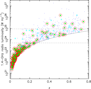
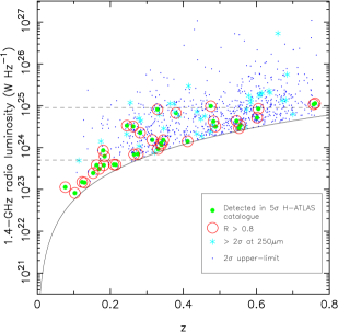
Figure 2: Radio luminosity of the radio-selected sample as a function of redshift split into the sub-1.5 $L_{K}^{*}$ sample (left) and super-1.5 $L_{K}^{*}$ (right). Sources nominally detected by Herschel (i.e. sources identified with H-ATLAS objects) are marked as filled green circles. If the association with the LAS galaxy is deemed `reliable', the object is also marked with a red open circle. Any source not identified with H-ATLAS object in the catalogue, but is detected down to the $2\sigma$ level (see Section 4.1 for how we define the $2\sigma$ level) in the 250-$\mu$m images, is shown as a light blue star for illustrative purposes only. Non-detections are marked with blue dots. The solid line corresponds to the nominal 5$\sigma$ flux cutoff in the NVSS of 2.25 mJy. Dashed horizontal lines show radio luminosities corresponding to (from bottom to top) the point at which the starburst radio luminosity function cuts off steeply (Sadler et al. 2002) and the expected luminosity for a maximal (4000 $M_{\odot}$ year^-1) starburst.

Next, we cross-correlated this radio catalogue with our base catalogue (see previous section) using the LAS positions on a 1^′′ best match basis. This process gave us a total of 1599 radio-detected sources in the Phase 1 area, of which 1110, or 69 per cent, had spectroscopic redshifts. Approximately 80 per cent of the spectroscopic redshifts are below $z=0.5$. The SDSS $r^{\prime}$-band limit accounts for the reduction of LAS identified radio sources from 3182 to 1599; $\sim$ 76 per cent of the dropouts have $K$ $>$ 17.0.

Next, we measured the size of all the cross-matched radio sources. If the source was compact in FIRST, we used the de-convolved major axis from the FIRST catalogue as the projected size of the radio source. The 1$\sigma$ source size error is given by:

$$\mathrm{Sigma}=10\,^{\prime\prime}\,\times\,\left(\frac{1}{SNR}+\frac{1}{75}\right)$$ (1)

where SNR is the signal-to-noise ratio of the FIRST source (Becker, White & Helfand 1995). If the de-convolved source size was less than 2$\sigma$ (equivalent to the 95 per cent contour) we took a 2$\sigma$ upper limit; this was the case for $\sim$ 13 per cent of the sources. The sizes of more complicated structures such as double-lobed radio sources were measured by calculating the projected distance between the peaks of the lobes. Where there was evidence for multiple lobes, the distance between the two furthest lobes from the host was recorded. There were 89 objects in which the NVSS emission was resolved out in FIRST. Such sources were not assigned sizes and were thus excluded from the analysis involving radio source sizes.

In order to calculate spectral indices, we cross-matched the filtered 1.4-GHz radio catalogue with 330 MHz GMRT radio catalogues and images, whose depth range from 3-10 mJy (Mauch et al. in preparation). Each match was checked manually by overlaying GMRT radio contours on LAS K-band images. A total of 726 sources were successfully matched. Upper limits on the spectral indices were calculated for the remaining sources (654) by substituting the GMRT flux by five times the local RMS. A further 219 radio sources do not have spectral indices or limits due to limited GMRT coverage of the Phase 1 area. This catalogue, which is a subset of the main radio catalogue described above, is only used in the analysis involving spectral indices.

The above processes gave us a catalogue which is flux-limited in the radio (by virtue of the original selection from the NVSS) and also magnitude-limited in the optical (we require a $K$-band identification and also require $r^{\prime}<22$). The result is that we have few (71) sources above $z>0.7$. The catalogue is also likely to be strongly biased against radio-detected quasars since we have excluded sources that appear point-like from our galaxy catalogue. This has the desirable effect that the measured FIR luminosities will tend not to be strongly affected by beaming of the radio jet and that any contamination of the fluxes measured at Herschel wavelengths by non-thermal emission might be expected to be limited (cf. the results of Hes, Barthel & Hoekstra 1995). Hereafter, the sources not identified with radio emission are referred to as comparison or non radio-detected sources while the sources identified with radio emission are referred to as radio-detected sources.

3.1 K-band luminosity cuts

In order to account for any stellar mass dependent relations, we calculate the $K$-band luminosity. The $K$-band luminosity is dominated by old stellar light (e.g. Best, Longair & Röettgering 1998; Simpson, Rawlings & Lacy 1999) and thus scales well with stellar mass. In order to enable us to compare radio galaxies with their mass equivalent non radio-detected counterparts, we use the absolute $K$-band magnitude.

Fig. 1 shows the absolute $K$ band magnitude versus redshift. Here we calculate the K-corrected and passive evolution corrected magnitude at $K$ using a GALAXEV starburst spectral energy distribution (see Bruzual & Charlot 2003) at $z=4$, with solar metallicity, allowing it to exponentially decay with $\tau=1$ Gyr. We apply this correction to both the radio sources and the comparison galaxies. We adopt a value of $-23.96$ for M${}^{*}_{K}$ (Smith, Loveday & Cross 2009; value calculated for our adopted cosmology) from which we calculate $L_{K}^{*}$ to be 7.87 $\times$ 10¹⁰ $L_{\astrosun}$. We separate the radio-selected sample into two magnitude bins, defined by M_K $>$ -24.4 (sub-1.5 $L_{K}^{*}$) and M${}_{K}<-24.4$ (super-1.5 $L_{K}^{*}$). For illustrative purposes only, we calculate the stellar mass boundary assuming a mass-to-light ratio of 0.6 (Kauffmann & Charlot 1998) and find it to be roughly 7.1$\times$10¹⁰ M_☉. The lower-luminosity sample contains 770 radio sources while the higher-luminosity sample contains 829 radio sources.

3.2 Radio luminosities

Fig. 2 shows 1.4-GHz radio luminosity versus redshift for our two $K$-band luminosity separated radio samples. Since less than half of the radio sources at 1.4-GHz are detected at 330 MHz, we adopt $\alpha=0.8$ when calculating the 1.4-GHz radio luminosity of all the radio sources, where $S\propto\nu^{-\alpha}$ for the K-correction in the radio luminosity calculations; $\alpha=0.8$ is a typical observed value for low-frequency selected objects, and we expect that the selection against point-like optical objects will tend to select against flat-spectrum radio sources. Indeed, the subset of sources with GMRT detections suggest that only $\sim$ 2 per cent of our sources have $\alpha<0$ and that $\alpha=0.8$ is a reasonable value for our sample.

It is clear from Fig. 2 that we probe a wide range of radio luminosities. At the low-luminosity, low redshift end ($z<0.2$), we expect from existing analysis of the local 1.4-GHz luminosity function (e.g. Sadler et al. 2002; Mauch & Sadler 2007) that the population will be dominated by star-forming galaxies rather than radio AGN, although a few AGN may still be present. The starburst luminosity function cuts off steeply above $5\times 10^{23}$ W Hz^-1 at 1.4-GHz, so we expect that most of the objects above this luminosity will be radio AGN. Thus, in our sub-1.5 $L_{K}^{*}$ radio sample there exist two populations; the low redshift, low luminosity starburst population and the higher redshift, higher luminosity radio AGN population.

The super-1.5 $L_{K}^{*}$ radio sample contains fewer sources below $5\times 10^{23}$ W Hz^-1 and are thus almost exclusively composed of radio AGN. As mentioned in Section 1, Best & Heckman (2012) calculated the HERG / LERG luminosity functions for the local Universe and found that HERGs begin to dominate above $10^{26}$ W Hz^-1. Thus, our samples will be dominated by LERGs, although significant numbers of HERGs may be present, particularly at lower masses.

4 The far-IR properties of the sample

4.1 Herschel flux density measurements

In this section we describe the properties of the sample in the FIR. Throughout this section, FIR flux densities in the SPIRE bands are measured directly from the background-subtracted, PSF-convolved H-ATLAS Phase 1 images described in Section 2, taking the best estimate of the flux density to be the value in the image at the pixel corresponding most closely to the LAS position of our targets, with errors estimated from the corresponding position in the noise map. As discussed by Pascale et al. (2010), PSF-convolved maps provide the maximum-likelihood estimate for the flux density of a single isolated point source at a given position in the presence of thermal noise; this remains a reasonable approximation if the correlations between the positions of multiple sources are small, as we expect in real data due to physical clustering of objects. We also extracted PACS flux densities and corresponding errors from the images at 100 and 160 $\mu$m using circular apertures appropriate for the PACS beam (respectively 15.0 and 22.5 arcsec) and using the appropriate aperture corrections, which take account of whether any map-pixels have been masked during the process of high-pass filtering of the bolometer timelines. We add an estimated absolute flux calibration uncertainty of 10 per cent (PACS) and 7 per cent (SPIRE) in quadrature to the errors measured from the maps for the purposes of fitting and stacking, as recommended in H-ATLAS documentation. To account for bright, extended objects, we use the flux densities in the Phase 1 5$\sigma$ catalogue, where available, in preference to our measured flux densities, even though our measured flux densities correlate well with the catalogued fluxes. To correct for confusion in the SPIRE maps, we subtract the mean flux density level of the whole PSF-convolved map from the flux density measurements of each source. This ensures that the mean of a randomly selected sample will be zero within the uncertainties.

Approximately 13.6 per cent of the radio sample (218 sources, which includes potential star-forming galaxies) is detected at the 5$\sigma$ limit demanded by the H-ATLAS source catalogue. This is broadly similar to the detection fraction found in H10. In order to give the reader a feel for the H-ATLAS $S/N$ distribution of the radio sample, we define a 2$\sigma$ rms value. Since the images at 250, 350 and 500 $\mu$m are seriously affected by confusion (as opposed to the PACS maps, which are not), we cannot use the 2$\sigma$ limit defined by simple Gaussian statistics (i.e twice the RMS). Instead, we follow Hardcastle et al. (2013) (hereafter, H13) and randomly sample a large number of points in the 250, 350 and 500 $\mu$m maps, selecting the flux value below which 97.7 per cent of the random fluxes lie as our 2$\sigma$ limit. This gives flux limits of 24.6, 26.5 and 25.6 mJy for the 250, 350 and 500-mm SPIRE maps respectively. Therefore, sources which have a $S/N>2$ at 250, 350 and 500 $\mu$m make up 18.9, 16.6 and 12.6 per cent of the sample, respectively.

We note that whether a source is `detected' or not plays no part in the following analysis, since we are interested in the sample properties taken as a whole. However, in some of the following plots the FIR luminosity of sources above 2$\sigma$ are shown as individual points for illustrative purposes only.

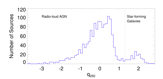
Figure 3: Histogram of $q_{250}$ values, defined in Eq. 2. We remove all sources with $q_{250}>1.3$, in order to ensure no star-forming objects are in our radio AGN sample. We note that many of the $q_{250}$ values are upper-limits, particularly below $q_{250}<1.3$.

4.2 250$\mu$m luminosity calculations

In H10, we calculated the integrated IR-luminosity of individual sources by assuming a spectral energy distribution (SED) with $T=26$ K and $\beta$ = 1.5 following Dye et al. (2010). In this paper, we follow a similar method to that of H10 with some key differences. Firstly, we assume $T=20$ K and $\beta$ = 1.8, best-fitting values derived for a similarly selected sample of radio galaxies by H13. Secondly, we calculate the FIR luminosity at 250 $\mu$m, rather than the integrated IR luminosity. This means that the isothermal model, and hence the assumed temperature only act as a K-correction factor in the determination of the 250 $\mu$m luminosity ($L_{250}$) of each source. Further, we note that at low redshifts, the calculated K-correction should have almost no effect on the 250 $\mu$m luminosity. The disadvantage of switching to the 250 $\mu$m luminosity is that we are no longer able to estimate the SFR. However, the relations which convert the integrated IR luminosity to a SFR are calibrated for star-forming galaxies (e.g. Kennicutt 1998) and thus may not be applicable to the temperature and luminosity range radio galaxies occupy in any case.

The Herschel SPIRE PSF has a FWHM of 18^′′ at 250 $\mu$m. This translates to linear sizes of $\sim$135 kpc at $z=0.8$, the redshift of our most distant objects. Therefore, the corresponding FIR luminosities and temperatures we measure apply not only to the host of the radio source but also to its immediate environment; this may include quiescent dust or star-formation in a companion or merging galaxy.

4.3 Removing star-forming galaxies

In order to remove star-forming galaxies from our sample, we calculate $q_{250}$ as follows,

$$q_{250}=\log_{10}(L_{\rm 250}/L_{1.4})$$ (2)

where $L_{250}$ is the K-corrected luminosity at 250 $\mu$m. This was done for the entire radio-detected sample. A histogram of the results is shown in Fig. 3. The far-infrared radio correlation (FIRC) has been shown to hold at 250 $\mu$m (Jarvis et al. 2010). The expected dispersion for sources on the far-infrared radio correlation (FIRC) is $1.4<q_{250}<2.1$ (Jarvis et al. 2010). Using Fig. 3, we choose to remove all sources with $q_{250}>1.3$ or where the upper limit on $q_{250}$ is $>1.3$, ensuring that no (or a negligible few) star-forming objects are in our subsequent radio AGN sample. This ensures that any source with the potential to be a star-forming object has been removed. Therefore, beyond this point star-forming objects play no further part in the catalogues / analysis unless explicitly stated.

Table 1: Mean bin flux densities and K-S probabilities that the Herschel fluxes of radio-detected objects in redshift bins are drawn from the background distribution, as a function of wavelength. Low probabilities (below 1 per cent) imply significant differences between the bin being considered and the distribution of flux densities measured from randomly selected positions in the sky, as described in the text. Sources on the FIRC are not included.

Radio	$z$ range	Objects	Mean bin flux density (mJy)					K-S probability (per cent)
Sample		in bin	SPIRE bands			PACS bands		SPIRE bands			PACS bands
			250 $\mu$m	350 $\mu$m	500 $\mu$m	100 $\mu$m	160 $\mu$m	250 $\mu$m	350 $\mu$m	500 $\mu$m	100 $\mu$m	160 $\mu$m
$<$1.5 $L_{K}^{*}$	0.00 – 0.15	92	$25.0\pm 0.8$	$9.8\pm 0.8$	$6.9\pm 0.9$	$36.7\pm 3.2$	$34.8\pm 3.9$	$<10^{-3}$	$<10^{-3}$	0.02	0.04	0.3
	0.15 – 0.25	90	$9.0\pm 0.7$	$3.1\pm 0.8$	$2.9\pm 0.9$	$12.8\pm 3.0$	$21.0\pm 3.8$	$<10^{-3}$	0.09	2.2	16.5	0.6
	0.25 – 0.40	182	$7.0\pm 0.5$	$1.3\pm 0.5$	$2.4\pm 0.6$	$12.1\pm 2.2$	$6.4\pm 2.8$	$<10^{-3}$	1.4	5.8	1.5	82.7
	0.40 – 0.50	78	$7.5\pm 0.7$	$2.8\pm 0.8$	$5.0\pm 1.0$	$1.6\pm 3.4$	$21.6\pm 4.2$	$<10^{-3}$	0.02	0.006	92.4	0.03
	0.50 – 0.60	75	$9.1\pm 0.7$	$3.9\pm 0.8$	$4.9\pm 1.0$	$9.5\pm 3.6$	$19.8\pm 4.4$	$<10^{-3}$	0.2	0.5	42.1	12.2
	0.60 – 0.80	113	$5.7\pm 0.6$	$2.2\pm 0.7$	$4.5\pm 0.8$	$1.7\pm 3.0$	$12.9\pm 3.8$	$<10^{-3}$	0.002	0.001	44.0	8.0
$>$1.5 $L_{K}^{*}$	0.00 – 0.15	11	$6.7\pm 1.9$	$4.6\pm 2.2$	$3.8\pm 2.5$	$3.2\pm 9.0$	$12.7\pm 11.0$	4.3	9.0	22.4	70.7	88.9
	0.15 – 0.25	40	$9.8\pm 1.0$	$3.2\pm 1.1$	$3.0\pm 1.3$	$25.4\pm 5.0$	$34.4\pm 6.3$	1.2	2.4	29.6	8.8	0.9
	0.25 – 0.40	236	$6.4\pm 0.4$	$2.3\pm 0.5$	$3.1\pm 0.5$	$6.6\pm 2.0$	$10.8\pm 2.5$	$<10^{-3}$	$<10^{-3}$	0.2	37.0	6.1
	0.40 – 0.50	140	$2.7\pm 0.5$	$-0.3\pm 0.6$	$1.1\pm 0.7$	$-1.5\pm 2.5$	$0.9\pm 3.1$	0.04	15.5	40.4	83.2	42.0
	0.50 – 0.60	178	$2.2\pm 0.5$	$-0.0\pm 0.5$	$1.3\pm 0.6$	$-4.6\pm 2.3$	$4.3\pm 2.9$	0.2	1.1	4.7	41.8	85.2
	0.60 – 0.80	210	$4.1\pm 0.4$	$1.3\pm 0.5$	$3.3\pm 0.6$	$3.1\pm 2.1$	$5.2\pm 2.7$	$<10^{-3}$	0.003	0.1	4.4	12.2

Table 2: Mean bin flux densities and K-S probabilities that the Herschel fluxes of radio-detected objects in radio luminosity bins are drawn from the background distribution, as a function of wavelength. Low probabilities (below 1 per cent) imply significant differences between the bin being considered and the distribution of flux densities measured from randomly selected positions in the sky, as described in the text. Sources on the FIRC are not included.

Radio	Range in	Objects	Mean bin flux density (mJy)					K-S probability (per cent)
Sample	log10($L_{1.4}$)	in bin	SPIRE bands			PACS bands		SPIRE bands			PACS bands
			250 $\mu$m	350 $\mu$m	500 $\mu$m	100 $\mu$m	160 $\mu$m	250 $\mu$m	350 $\mu$m	500 $\mu$m	100 $\mu$m	160 $\mu$m
$<$1.5 $L_{K}^{*}$	21.0 – 23.7	114	$22.3\pm 0.7$	$8.1\pm 0.7$	$5.1\pm 0.8$	$34.0\pm 2.8$	$30.1\pm 3.4$	$<10^{-3}$	$<10^{-3}$	0.07	0.005	0.10
	23.7 – 24.3	140	$4.3\pm 0.5$	$-0.7\pm 0.6$	$1.1\pm 0.7$	$7.8\pm 2.5$	$9.0\pm 3.2$	$<10^{-3}$	17.4	41.9	1.5	51.3
	24.3 – 24.6	115	$9.2\pm 0.6$	$2.2\pm 0.7$	$3.3\pm 0.8$	$9.2\pm 2.8$	$21.5\pm 3.4$	$<10^{-3}$	0.8	0.6	56.4	3.0
	24.6 – 25.0	116	$8.8\pm 0.6$	$5.1\pm 0.7$	$6.4\pm 0.8$	$8.0\pm 2.9$	$13.6\pm 3.7$	$<10^{-3}$	$<10^{-3}$	0.002	38.4	20.5
	25.0 – 25.6	99	$7.3\pm 0.6$	$2.9\pm 0.7$	$3.9\pm 0.8$	$3.7\pm 3.1$	$15.5\pm 3.8$	$<10^{-3}$	0.2	0.007	36.9	4.7
	25.6 – 27.3	46	$7.7\pm 1.0$	$4.9\pm 1.1$	$7.7\pm 1.3$	$9.2\pm 4.4$	$13.4\pm 5.4$	0.003	0.02	0.05	5.2	18.2
$>$1.5 $L_{K}^{*}$	21.0 – 23.7	13	$12.6\pm 1.8$	$6.4\pm 2.0$	$3.9\pm 2.3$	$7.3\pm 8.4$	$19.4\pm 10.2$	1.2	8.0	7.5	59.3	25.9
	23.7 – 24.3	128	$5.2\pm 0.6$	$1.2\pm 0.6$	$1.6\pm 0.7$	$6.8\pm 2.8$	$12.4\pm 3.4$	0.002	0.3	13.2	8.4	5.9
	24.3 – 24.6	159	$5.1\pm 0.5$	$3.0\pm 0.6$	$4.9\pm 0.7$	$1.6\pm 2.4$	$9.2\pm 3.0$	0.009	$<10^{-3}$	0.03	67.8	16.1
	24.6 – 25.0	268	$3.2\pm 0.4$	$-0.3\pm 0.4$	$0.6\pm 0.5$	$3.0\pm 1.9$	$6.0\pm 2.4$	0.006	0.9	34.0	56.0	51.2
	25.0 – 25.6	183	$4.5\pm 0.5$	$1.5\pm 0.5$	$3.7\pm 0.6$	$-1.3\pm 2.2$	$5.3\pm 2.8$	$<10^{-3}$	0.06	0.2	56.6	1.3
	25.6 – 27.3	64	$3.9\pm 0.8$	$0.8\pm 0.9$	$1.6\pm 1.0$	$7.1\pm 3.5$	$2.5\pm 4.6$	0.008	0.2	36.3	0.9	57.0

4.4 Stacking analysis

Since the vast majority of our radio AGN ($\sim 95$ per cent) are undetected at the 5$\sigma$ limit of the Phase 1 catalogue, we need to use statistical methods to calculate the properties of the source population. We elected to stack the sample using the 100, 160, 250, 350 and 500 $\mu$m H-ATLAS maps in bins of redshift and radio luminosity which range from $0.01<z<0.8$ and $21.0<{\rm log}_{10}$($L_{1.4}$) $<27.3$. We use the same bin sizes, in both radio luminosity and redshift, across both $K$-band luminosity separated samples in order to facilitate comparisons. Individual bin sizes were chosen so as to keep as many bins distinguished from the background as possible.

To establish quantitatively whether sources in the bins were significantly detected, we measured flux densities from 100,000 randomly chosen positions in the field; a Kolmogorov-Smirnov (K-S) test could then be used to see whether the sources from our sample were consistent with being drawn from a population defined by the random positions. Using a K-S test rather than simply considering the calculated uncertainties on the measured fluxes allows us to account for the non-Gaussian nature of the noise as a result of confusion. If the fluxes in any given bin are significantly distinguished from the background on a K-S test and have a mean flux density higher than that of the underlying noise (which should be zero, see Section 4.1), we can calculate the stacked luminosity using all the objects in that bin in the knowledge that the resulting value is not simply noise.

The results from this analysis are shown in Tables 1 and 2. Both tables show the results for the $K$-band luminosity separated radio samples. Sources on the FIRC have been removed. As is evident from Tables 1 and 2, most of the SPIRE bins are detected at the 95 per cent confidence level (i.e. there is a $<5$ per cent chance that the flux distribution has been randomly drawn from the same underlying distribution as the background). However, the PACS bins are mostly indistinguishable from the background. This is the result of the lower sensitivity of the PACS data. It is also clear that the K-S probabilities are almost always lower at 250 $\mu$m than at any other band, with all of the bins at 250 $\mu$m detected above the 99 per cent confidence level or better, except for the lowest redshift bin of the super-1.5 $L^{*}_{K}$ sample. The higher sensitivity and smaller beam size at 250 $\mu$m are likely explanations for this. Indeed, if one excludes those radio sources which are also in the 5$\sigma$ H-ATLAS catalogue from the K-S test, all the SPIRE bins are detected at the 96 per cent level or better except the super-$L^{*}_{K}$ $0.15<z<0.25$ bin, which is detected at the 83.8 per cent level. This provides further justification for calculating the rest-frame luminosity at 250 $\mu$m. The KS probabilities produced by the comparison sources are not shown, but all the bins at 250 $\mu$m were detected above the 99 per cent confidence level or better.

In order to calculate stacked luminosities, we calculate the weighted average of $L_{250}$ for each radio luminosity or redshift bin. Individual sources are weighted using the reciprocal of the square of the error extracted from the 250 $\mu$m noise map. In order to calculate errors on the stacked luminosity, we use the bootstrap method with replacement. This involves randomly selecting a subsample from the relevant bin, while ensuring that the total number of sources in that bin remains constant. This implies that the same source may be selected more than once and others omitted completely. From this new sample, a weighted $L_{250}$ value is calculated and stored. We repeat the process 300 times in order to get a distribution of weighted $L_{250}$ values. From this distribution, we select the 16^th and 84^th percentiles as our lower and upper limits respectively. The advantage of bootstrapping is that no assumption is made on the shape of the luminosity distribution; instead, we use the distribution of the sample to calculate 1$\sigma$ errors. This automatically takes all sources of intrinsic dispersion, such as redshift errors and flux errors, into account. The errors plotted in all subsequent FIR luminosity plots are the 1$\sigma$ uncertainties derived from bootstrapping.

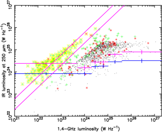
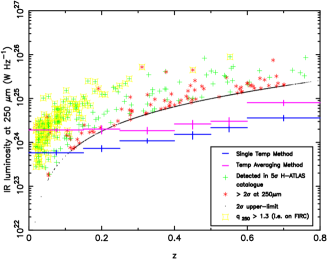
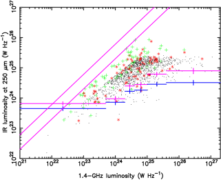
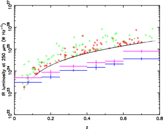
Figure 4: Stacked infrared luminosity at 250 $\mu$m as a function of (left) radio luminosity and (right) redshift. (Top) Radio sources on the FIRC are included, (bottom) radio sources on the FIRC are not included. Plotted sources, which are shown for illustrative purposes only, have had their luminosities calculated using the $T=20$ K isothermal model described in the text. FIR-luminosities calculated via the single temperature model / temperature averaging method are in blue / magenta). Green crosses are 5$\sigma$ detected sources defined by the H-ATLAS Phase 1 catalogue whilst red stars and black points are the $>$ 2$\sigma$ and 2-$\sigma$ upper-limits, respectively. Those sources with $q_{250}>1.3$ are identified with yellow boxes. The upper and lower magenta lines are $q_{250}=1.78$ (the FIRC as defined by Jarvis et al. 2010) and $q_{250}=1.3$ respectively.

4.5 Averaging dust temperatures

In Section 4.2, we calculated the luminosity at 250 $\mu$m using an isothermal model with $T=20$ K. Obviously, such a model contains no information on the dust temperature but we know from H13 that a wide range of temperatures are observed in the radio selected objects. In order to gain some constraints on the temperature, we calculated a weighted average of the fitted temperatures of the sources in each bin. To this end, we take a simple $\chi^{2}$ approach. We cycle through temperatures between 5-55 K and fit to all the five Herschel flux bands, allowing only the normalization of each source to vary (assuming a modified blackbody SED with $\beta$ $=$ 1.8). For each temperature step, we sum the $\chi^{2}$ value produced by each source. This results in a $\chi^{2}$ distribution as a function of temperature from which we pick the temperature with the lowest $\chi^{2}$ value. The errors are calculated by finding the range where $\Delta\chi^{2}=1$.

Although our primary aim is to extract temperature information from each bin, we can use this temperature to calculate a K-corrected luminosity at 250 $\mu$m for every source in the bin, again allowing the normalization of each source to vary. It is important to stress here that the normalization of each source is determined from all five Herschel bands, so the resulting $S_{250}$ value (and therefore the $L_{250}$) may differ substantially from the nominal $S_{250}$ value in the 250 $\mu$m map. Confusion bias is likely to affect the 500 $\mu$m more strongly than any other due to the increased size of the beam and higher noise levels. To ensure that our temperatures were not strongly biased by the inclusion of this band, we computed all the temperature estimates presented in the paper without the 500 $\mu$m band and found that the derived temperatures were not significantly different. In the next section we compare the $L_{250}$ output of the $T=20$ K isothermal model to that of the temperature averaging method described above.

4.6 FIR luminosities: Comparison of methods

In this section we compare the luminosities of the single temperature and temperature averaging models. To do this, we calculate the stacked luminosity at 250 $\mu$m of our radio-selected samples as a function of redshift and radio luminosity, the results of which are shown in Fig. 4 (we note that all the bins are significantly detected with respect to the background). The upper plots include the sources on the FIRC whilst the lower plots exclude such sources. The luminosities calculated using the $T=20$ K isothermal model are shown by the stacks in blue while the luminosities calculated via the temperature averaging method are shown by the stacks in magenta. All the plotted sources in Fig. 4 have had their luminosities calculated assuming the single temperature model and are shown for illustrative purposes only. In the top left panel of Fig. 4, it is clear that the sources on the FIRC are well separated from the radio AGN population. This is not surprising given the clean separation observed in Fig. 3, nevertheless, it is encouraging to observe this bi-modality as a function of radio luminosity.

Turning first to the upper plots in Fig. 4, which contain the star-forming sources, we see that the luminosities from both methods do not agree particularly well. The temperature averaging method produces fitted temperatures ranging from 17-30 K, with all but the highest redshift and radio luminosity stacks having fitted temperatures above $T=20$ K. Furthermore, the luminosities derived from the temperature averaging method appear systematically higher than the ones observed for the single temperature model. This is because the individual sources in the temperature averaging method are free to find their own normalizations based on information in all the Herschel bands. This normalization value is usually higher where star-forming objects are included, probably due to the flux contained in the PACS bands. If one removes the hot, bright low redshift star-forming objects (Fig. 4: lower plots), the luminosity difference between both methods decreases significantly. Nevertheless, there are still some systematic differences between both methods.

When investigating the FIR luminosities of radio-detected and non radio-detected galaxies, we will not use the temperature averaging method. This is because under that method, the 250 $\mu$m luminosity of any given source is dependent on the luminosities of others in that bin though the temperature estimation. The $T=20$ K isothermal model described above is not susceptible to such correlations, as a single temperature and independent flux density values ($S_{250}$) are used when calculating individual luminosities. The systematic differences observed between methods suggest that the errors on the absolute luminosities of both methods have probably been underestimated, since they are highly dependent on the chosen method. However, our science conclusions will depend on the relative luminosity between samples (i.e between radio-detected and non radio-detected galaxies). Therefore, in so far as $T=20$ K is a reasonable temperature estimate for the K-correction of our sample, the single temperature method described in Section 4.2 is sufficient for the investigation of luminosity differences between samples. All the following plots have had their IR luminosities calculated using the isothermal $T=20$ K model, while the temperatures have been generated using the temperature averaging method.

4.7 What does the luminosity at 250 $\mu$m trace?

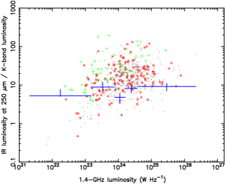
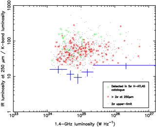
Figure 5: Stacked FIR luminosity at 250 $\mu$m (W Hz^-1) divided by the K-band luminosity (W Hz^-1), as a function of 1.4-GHz radio luminosity for sources $z<0.4$ (left) and $z>0.4$ (right). Sources on the FIRC are not included. Note the different axial ranges present in both plots.

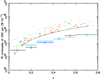
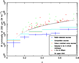
Figure 6: Stacked FIR luminosity at 250 $\mu$m as a function of redshift. Stacks shown in blue, cyan and orange are from the radio-detected, non radio-detected and g^′- r^′ colour matched non radio-detected galaxy samples, respectively. Left and right plots contain the sub-1.5 $L_{K}^{*}$ and super-1.5 $L_{K}^{*}$ samples, respectively. Sources on the FIRC are not included. In some redshift bins, the colour-matched non radio-detected stacks are not clearly visible because the stacked luminosities are very similar to the unmatched non radio-detected luminosities.

Using the rest-frame luminosity at 250 $\mu$m minimises the dispersion in our FIR luminosity calculations, but what does it physically trace? First, we must tackle the issue of AGN contamination from (1) synchrotron emission and (2) hot dusty tori. The first of these points has largely been addressed in the text above: point sources which may be face-on quasars were filtered from the catalogue at an early stage and sources which have radio spectral indices below 0 are expected to make up less than 2 per cent of the radio source catalogue (see Section 3.2). As for dusty tori surrounding AGN, they peak in the mid-IR. When the required mid-IR data are available, which is not the case for our sample at present, decompositions of the SEDs of radio-detected and non radio-detected AGN tend to show that observer-frame Herschel SPIRE bands are dominated by cool dust rather than by the torus component, even for powerful AGN with luminous tori (e.g. Barthel et al. 2012; Del Moro et al. 2013). Since the luminosity calculations rely solely on the 250 $\mu$m band, we do not expect any AGN contamination. In our temperature averaging method, we use PACS 100 $\mu$m data which at $z=0.8$ (the maximum redshift in our sample) corresponds to a rest-frame wavelength of 55.5 $\mu$m. Although there is some potential for AGN contamination here we note that broadly, the torus luminosity scales with the radio luminosity (Hardcastle, Evans & Croston 2009), and the vast majority of our sources are below the threshold for `powerful radio galaxies' ($\sim$1$\times$10²⁶ WHz^-1) where bright tori might be expected. In addition, the noise in the PACS bands mean that PACS photometry is lightly weighted relative to the SPIRE bands in the temperature fitting method. Therefore, we do not believe that our luminosities or temperatures have been significantly affected by AGN components.

In reality, dust exists at a range of temperatures whose integrated luminosity is often fitted by one, or two, modified isothermal blackbodies (e.g. Dunne et al. 2011). This has been driven by an inability to determine, and thus constrain, the physical composition and / or temperature distribution of the dust, which would allow more sophisticated models to be used. Nevertheless, for the purposes of understanding what the luminosity at 250 $\mu$m represents in our sample, it is instructive to assume a two-temperature blackbody model. Such models attempt to separate warm dust, which is expected to dominated the IR luminosity output, from the cold dust, which is expected to dominate the dust mass (Dunne et al. 2011).

In general, priors for the cold and warm components range from 10-25 K and 30-60 K respectively (e.g. da Cunha, Charlot & Elbaz 2008). At 250 $\mu$m, both components may contribute to the total luminosity. For example, assuming a warm dust component with a temperature of 32 K and a cold dust component with a temperature of 15 K, with the latter contributing 90 per cent of the total dust mass (typical for sources detected in H-ATLAS; Dunne et al. 2011), we find that both components would contribute equally to $L_{250}$. Although other temperature combinations are possible within the range of temperature priors quoted above, this demonstrates our inability to state unambiguously that $L_{250}$ is dominated by either warm or cold dust. This degeneracy is important, as it is likely that the warm dust is the component that traces heating by on-going star-formation. Given the quality of our data, we make no attempt to partition $L_{250}$ into a warm and cold component, although, in Section 5.2, we attempt to use the temperatures generated from the temperature averaging method to shed light on this degeneracy.

5 Results

5.1 FIR properties of the K-band luminosity-separated radio galaxies

Galaxy mass is a fundamental indicator of host galaxy properties. This is especially true of radio galaxies. There is increasing evidence for fundamental mass-dependent differences in the radio luminosity functions, accretion rates and possibly fuelling mechanisms of radio galaxies (c.f. Best et al. 2005; Best & Heckman 2012). For these reasons, we investigate the luminosity at 250 $\mu$m of our radio AGN as a function of the K-band luminosity (a proxy for stellar mass), as well as redshift and radio luminosity.

In the lower left-hand panel of Fig. 4, it is clear that $L_{250}$ increases with the 1.4-GHz radio luminosity. However, such a relation may be the result of observational selection effects. For example, the incompleteness that arises from the flux-limited nature of the NVSS means that we have not identified low radio-luminosity sources at high redshift. The inclusion of such sources would likely flatten the observed relation since we expect these sources to have systematically higher $L_{250}$ values than their lower redshift counterparts (the FIR luminosity of the galaxy population as a whole increases with redshift for the redshift range under discussion; Dunne et al. 2011). A similar select effect is at work with respect to the K-band magnitude-limited LAS images. Such a limit means that we do not detect low-luminosity (i.e. low-mass) radio sources at high redshift (see Fig. 1). In order to remove any stellar-mass bias, we divide $L_{250}$ by $L_{K}$ in Fig. 5. This new value can be thought of as the specific FIR luminosity at 250 $\mu$m. To limit the redshift bias, we plot the sources below and above $z=0.4$ in the left and right-hand panels of Fig. 5, respectively. The sizes of the stacked bins were chosen so as to ensure that an equal number of radio sources were in each stack. Due to the flux limited nature of our radio-selected sample, we do not have any sources below 1$\times$10²⁴ WHz^-1 in the $z>0.4$ sample. The best fit (assuming a line with a gradient of zero) specific FIR luminosity at 250 $\mu$m of the $z<0.4$ and $z>0.4$ samples are 6.5$\pm$1.7 and 13.4$\pm$3.9 respectively. Nevertheless, it is clear that any relation between $L_{250}$ and 1.4-GHz radio luminosity disappears after these corrections, although the FIR luminosities of the $z>0.4$ sources are systematically higher than that of the $z<0.4$ sources. This implies that the strength of a galaxy's radio emission has little or no bearing on its specific FIR luminosity at 250 $\mu$m.

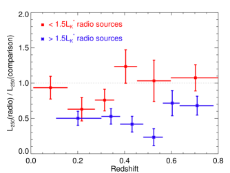
Figure 7: Plotted is the ratio of the stacked $L_{250}$ values of radio-detected and non radio-detected galaxies against redshift. The radio sample is divided into sub (red) and super (blue) 1.5 $L_{K}^{*}$ samples. Stack sizes are chosen to ensure each bin contains the same number of radio sources.

Next, we compare the IR luminosities of the radio-detected sources against their non radio-detected counterparts. Here, it is important to ensure that any FIR luminosity deviation between the samples is not simply the result of differing optical colours. The average K-corrected g^′ - r^′ colours of the sub-1.5 $L_{K}^{*}$ and super-1.5 $L_{K}^{*}$ radio-detected samples are 0.83 and 0.90 respectively, while average colours of the sub-1.5 $L_{K}^{*}$ and super-1.5 $L_{K}^{*}$ non radio-detected samples are 0.75 and 0.91 respectively. Thus, while the average colours of the super-1.5 $L_{K}^{*}$ samples match up well, the sub-1.5 $L_{K}^{*}$ radio-detected galaxies have redder colours than their non radio-detected counterparts. In order to take colour into account, we filter our sub and super-1.5 $L_{K}^{*}$ comparison samples so as to match the distribution of g^′ - r^′ colours observed in the sub and super-1.5 $L_{K}^{*}$ radio-detected samples. For each subsample, we do this by first imposing a global g^′ - r^′ colour cut, defined by the middle 98 per cent of the radio galaxy colour distribution; this removes any outliers in the radio-detected and comparison samples. Next, we randomly discard one per cent of the galaxies in the comparison sample and then run a K-S test to establish how well the new colour distribution matches to the radio-detected distribution. Discarding a different one per cent and repeating the process $N$ times, where $N$ is the number of comparison sources in the sample, allows us to select the best-matching reduced catalogue. After selecting the best matching catalogue, we again discard one per cent of the remaining sources in the comparison sample and repeat the entire process. This is done until the null hypothesis probability returned by the K-S test exceeds 10 per cent. This colour-matching process is performed for the sources in each redshift bin separately. The main disadvantage of such a method is the potential loss of large fractions of the original comparison sample. We lose $\sim$ 55 per cent of the comparison sources in the sub-1.5 $L_{K}^{*}$ sample; however, this still leaves us with over 136,000 sources. In the super-1.5 $L_{K}^{*}$ comparison sample, we only lose $\sim$ 6 per cent of the sources leaving us with over 26,000 sources. In Fig. 6, we plot $L_{250}$ versus redshift. The radio galaxy stacks are plotted in dark blue whilst the comparison galaxy stacks are plotted in cyan. Sources on the FIRC have been excluded from this plot. The stacks shown in orange are generated using the colour matched comparison samples. Hereafter, `colour-matched' samples refer to the comparison samples which have undergone the matching process described above.

It is immediately apparent from Fig. 6 that both the stacked radio and comparison samples show an increase in $L_{250}$ with redshift. This is consistent with the picture that dust masses and star-formation activity were higher in the past (e.g. Dunne et al. 2011). Turning to the differences between the K-band luminosity separated radio-galaxies, there is a suggestion that the sources in the sub-1.5 $L_{K}^{*}$ sample have higher FIR luminosities than those in the super-1.5 $L_{K}^{*}$ sample. In order to quantify this difference, we divide the $L_{250}$ values of the sub-1.5 $L_{K}^{*}$ sample, shown in Fig. 6, by the equivalent $L_{250}$ values of the super-1.5 $L_{K}^{*}$ sample. We find the sub-1.5 $L_{K}^{*}$ radio-detected sample to be 1.53$\pm$0.32 times as luminous as the super-1.5 $L_{K}^{*}$ radio-detected sample. Therefore, although there is some evidence for higher FIR luminosities in the sub-1.5 $L_{K}^{*}$ sample, this result is not significant due to the large errors.

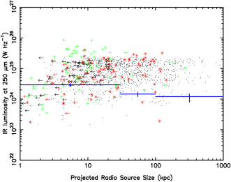
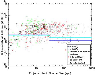
Figure 8: FIR luminosity at 250 $\mu$m versus the projected radio source size. Radio sources on the FIRC are excluded. On the left-hand panel, we plot the stacked values for the entire radio-detected sample. On the right-hand panel, we plot the stacked values for the sub (cyan) and super (blue) 1.5 $L_{K}^{*}$ radio-detected samples. Plotted sources are shown for illustrative purposes only. Green crosses are 5$\sigma$ detected sources defined by the H-ATLAS Phase 1 catalogue whilst red stars / black points are the $>$ 2$\sigma$ / 2-$\sigma$ upper-limits respectively. The arrows represent the upper limits on the sizes of the radio sources.

In order to judge, quantitatively, whether there is any difference between the radio-detected and comparison samples, we divide the $L_{250}$ values of the the radio-selected stacks by the colour-matched comparison stacks and show the results in Fig. 7. The sizes of the stacked bins were chosen so as to ensure that an equal number of radio sources were in each stack. However, it is important to note several significant caveats before interpreting the results. Firstly, because the NVSS is a flux-limited survey, we do not have high-redshift, low-luminosity radio sources in our sample: i.e, as we move to higher redshifts, we are preferentially selecting powerful radio AGN and placing any low-luminosity radio galaxies in the comparison sample. Secondly, since our base galaxy catalogue is magnitude limited in the $K$ and $r^{\prime}$ bands, we become progressively incomplete with increasing redshift, losing faint and / or low-mass sources. Nonetheless, it is important to note that the radio and comparison samples have been selected from the same parent catalogue.

Fitting a line with a gradient of zero, we find the best fitting line for the sub-1.5 $L_{K}^{*}$ radio-detected sample is 0.89$\pm$0.18 times the FIR luminosity at 250 $\mu$m of the colour matched comparison sample. Thus, being radio-detected is not associated with higher luminosities at 250 $\mu$m. This is markedly different from what we see with the super-1.5 $L_{K}^{*}$ sample, which is significantly better constrained. We find the best fitting line for this sample to be 0.49$\pm$0.12 times the FIR luminosity at 250 $\mu$m of the colour matched comparison sample. Thus, it is clear that super-1.5 $L_{K}^{*}$ radio-galaxies show a strong 250 $\mu$m luminosity deficit with respect to their non radio-detected counterparts. We discuss the significance of the above results in Section 6.

5.2 FIR emission and radio source sizes

In Fig. 8 we plot $L_{250}$ versus the projected radio source size. The size of the radio source can be thought of as a rough proxy for the age of the radio source (e.g. Kaiser, Dennett-Thorpe & Alexander 1997). Sources on the FIRC have been excluded from this plot. The sizes of the stacked bins were chosen so as to keep all the radio sources with poorly constrained projected sizes in the first bin (i.e. $<$ 30 kpc). All the bins are significantly detected on a K-S test with respect to the background. On the left-hand panel of Fig. 8, we plot the results using the entire radio-detected sample with radio sizes. There is a clear indication that the luminosity at 250 $\mu$m falls with increasing source size. The null hypothesis, that $L_{250}$ is independent of radio size, is rejected at the 95 per cent confidence level. However, we must first discount the possibility that this fall in FIR luminosity is due to observational selection effects. Such an effect could be orchestrated if `compact' radio sources ($<$ 30 kpc) were at higher redshifts than their more `extended' counterparts ($>$ 30 kpc), during which FIR luminosities of all sources were higher, or at higher radio luminosities where the FIR luminosities of this sample are higher (see left-hand side of Fig. 4). However, the sub-30 kpc radio sources are slightly biased towards the low-redshift and low radio-luminosity ends compared to the super-30 kpc sample.

To help elucidate the origin of the FIR excess at small radio source sizes, we calculate the `best-fit' temperature, obtained using the temperature averaging method described in Section 4.5, for compact and extended radio sources. We find the fitted temperatures of compact and extended radio galaxies are 27.1$\pm$0.3 K and 13.1$\pm$0.3 K respectively. The higher temperatures are probably due to enhanced inter-stellar radiation fields (ISRF) heating cool dust. The source of this heating is likely to be enhanced levels of, possibly jet-induced or merger associated star-formation.

On the right-hand panel of Fig. 8, we separate the sample using the $K$-band luminosity. The super-1.5 $L_{K}^{*}$ and sub-1.5 $L_{K}^{*}$ radio galaxy stacks are shown in blue and cyan, respectively. Due to the sparsity of extended radio sources in the sub-1.5 $L_{K}^{*}$ sample, we only plot two stacks divided at 30 kpc. It is clear that both samples show a fall in $L_{250}$ with increasing radio source size, although the super-1.5 $L_{K}^{*}$ sample dominates this trend. We discuss the implications of these results in Section 6.

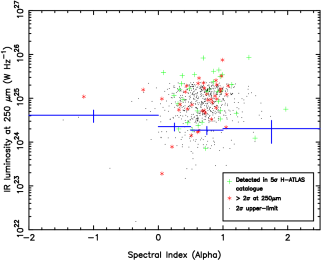
Figure 9: FIR luminosity at 250 $\mu$m versus the radio spectral index ($S\propto\nu^{-\alpha}$) for the subset of NVSS-detected sources (1.4-GHz) with GMRT detections (330 MHz).

5.3 FIR emission and spectral indices

The large survey at 330 MHz performed by the GMRT over the H-ATLAS Phase 1 fields (Mauch et al. in preparation) allows us to determine whether spectral indices are related to FIR luminosity. Spectral indices can be thought of as another rough proxy for radio source age. This is because, during the lifetime of a radio source, the electrons with the highest energies in a homogeneous magnetic field will radiate energy at a faster rate than their lower energy counterparts. This leads to a steepening of the spectral index at high frequencies. Thus, we might expect a negative relation between FIR luminosity and spectral index, if the radio source is somehow synchronised with the onset of star-forming activity.

In Fig. 9, we plot $L_{250}$ versus spectral index for the subset of radio sources with detections at 330 MHz. Excluding flat spectrum sources whose FIR emission may be contaminated by non-thermal emission ($\alpha<0$), we find no evidence for any relation between spectral index and $L_{250}$ in our sample of radio galaxies. The lack of a negative relation implies that either the star-forming and radio AGN activity are not well (or at all) synchronised in the current sample of radio galaxies or that spectral indices do not represent a good proxy for the age of our radio galaxies. It is also possible that the frequency range over which the spectral index is calculated is too low to see a relation between electron ageing and star formation. The addition of further data at radio frequencies, with which the shape of the spectral distribution could be reconstructed and thus modelled, may allow one to distinguish between the cases described above.

6 Discussion

The most obvious trend observed in both the stacked radio-detected and non radio-detected galaxy samples is the increase in the rest-frame luminosity at 250 $\mu$m with redshift. This is at least qualitatively consistent with previous results suggesting that dust masses and star-formation rates evolve strongly with redshift (e.g. Dunne et al. 2011).

Perhaps the most interesting result from Section 5 is the different behaviour of the sub and super-1.5 $L_{K}^{*}$ radio-detected galaxies with respect to their K-band and g^′- r^′ matched non radio-detected galaxies. While the 250 $\mu$m luminosity of the sub-1.5 $L_{K}^{*}$ radio-detected sample is indistinguishable from its matched comparison sample, the super-1.5 $L_{K}^{*}$ radio-detected sample shows a strong FIR luminosity deficit with respect to its matched comparison sample. However, what does a deficit at 250 $\mu$m tell us about the physical properties of the host systems?

The answer may depend on the fitted isothermal dust temperature. If the dust temperature of two matched samples are similar, any differences in the FIR luminosity will likely be due to differing dust masses. However, if the dust temperature of both samples differ greatly, then any differences in the FIR luminosity will likely be due to differing SFRs. To calculate the dust temperature of the radio-detected and comparison samples, we use the temperatures generated by the temperature averaging method described in Section 4.5. The primary drawback of using this method is that a small number of bright, and possibly warm sources may dominate the $\chi^{2}$ fitting, resulting in higher temperatures than one would expect by simple averaging. This implies that a minority of sources may be responsible for the majority of the temperature difference observed between two samples.

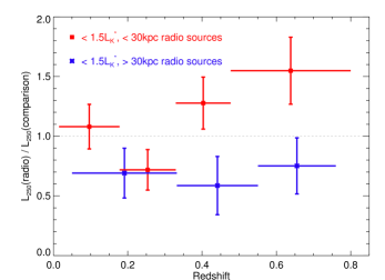
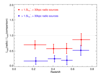
Figure 10: Stacked luminosities at 250 $\mu$m of the radio-detected samples divided by the colour-matched comparison samples. The sub-1.5 $L_{K}^{*}$ (left) and super-1.5 $L_{K}^{*}$ (right) radio-detected samples are separated into compact ($<$30 kpc) and extended ($>$30 kpc) radio galaxies. The red stacks represent the $<$30 kpc samples while the blue stacks represent the $>$30 kpc samples.

Turning first to the sub-1.5 $L_{K}^{*}$ radio-detected results, we find that the fitted temperatures of the radio-detected and non radio-detected samples are 20.5$\pm$0.5 K and 19.0$\pm$0.2 K, respectively. The combination of similar FIR luminosities and dust temperatures can be interpreted in several ways. For example it may simply mean that the radio jets, or the mechanism that leads to radio emission, are not strongly coupled to the dust reservoirs in all sub-1.5 $L_{K}^{*}$ galaxies. Alternatively, it is possible the radio-detected sample contains at least two distinct populations, with different FIR luminosities, which are not well separated by stellar mass alone. As discussed in Section 1, HERGs, which tend to be hosted in lower-mass galaxies, are expected to be triggered as a result of on-going gas-rich major mergers. We might then expect the radio sources in this sample to show a strong 250 $\mu$m luminosity excess due to a combination of increased star-formation and higher dust masses. However, HERGs dominate the radio luminosity function only above $\sim$10²⁶ WHz^-1 (Best & Heckman 2012), well above the luminosity of most of the sources in this sample. Thus, the sub-1.5 $L_{K}^{*}$ radio-detected sample is likely to contain a mixture of HERGs and LERGs. This makes it difficult to be certain that the null result is due to similar dust masses, as the presence of a small number of HERGs would render this interpretation invalid. Nevertheless, if one takes the sub-1.5 $L_{K}^{*}$ radio-detected population as a whole, it is clear that there is no evidence for differing FIR luminosities or (at least isothermal) dust temperatures.

The super-1.5 $L_{K}^{*}$ radio-detected sample, which we expect to be dominated by LERGs, shows a clear FIR luminosity deficit when compared to its colour-matched comparison sample. The suggestion here is that being radio-detected results in lower FIR luminosities. The fitted temperatures of the radio-detected and comparison sample are 16.2$\pm$0.5 K and 21.2$\pm$0.2 K respectively, implying that the observed differences may be due to a combination of lower dust masses and SFRs. One of the most obvious interpretations is that radio-jets directly destroy dust or inhibit star formation in these galaxies. If this were the case, we might expect a negative relation between the mechanical heating of the ISM by the jet (which itself is dependent on the 1.4-GHz radio luminosity) and $L_{250}$. However, we do not have the data to calculate mechanical heating caused by the jet. The lack of a negative relation between the specific 250 $\mu$m luminosity and 1.4-GHz radio luminosity, suggests that a causal connection between the radio jet and the luminosity deficit at 250 $\mu$m is unlikely, although evolution in $L_{1.4}$ may have washed out the effect. It is difficult to imagine hot, ionised radio-jets coupling efficiently to cold, neutral dust. If such a mechanism was real and ubiquitous, we might have expected to also see a $L_{250}$ deficit in the sub-1.5 $L_{K}^{*}$ radio-detected sample. That we do not suggest we must look elsewhere for a potential solution.

All massive galaxies sit at the bottom of large, dense and hot potential wells. However, what distinguishes radio-detected systems from their non radio-detected counterparts is that they inhabit the richest, hottest and densest of these environments. This is both because the radio activity is thought to be fuelled by the hot gas from the IGM (see Section 1) and because hot gas is required to confine the radio lobes. This hot gas may ultimately lead to a suppression of the total dust content of any galaxy embedded in this environment. Radio jets are known to drive shocks in the halos of their host galaxies, heating them (e.g. Croston et al. 2009). This heating has been used to solve the so called `cooling flow problem', where only small amounts of cold gas are observed to condense out of hot-gas halos despite radiative cooling timescales which are much less than the age of the host (McNamara & Nulsen 2012). This leads to lower star-formation rates and also lower dust production rates. In addition, the hot gas may directly destroy, or simply suppress the formation of dust particles inside the galaxy though sputtering (Draine & Salpeter 1979). Further, any in-falling galaxy is likely to be ram-pressure stripped of its gas and dust content by the hot gas, limiting the alternative sources of cold gas and dust available to galaxies embedded in this environment (see Abramson et al. 2011 and Vollmer et al. 2012 for examples of ram stripping in the Virgo cluster). Thus, the tendency of massive ($>$1.5 $L_{K}^{*}$) radio galaxies to inhabit rich environments may explain the implied lower dust masses and SFRs observed in these systems and the lack of such a result in the sub-1.5 $L_{K}^{*}$ radio galaxies.

Next, we turn to the results based on the radio source size. First, we note that the dust temperatures of compact radio sources, whether they are in the sub or super-1.5 $L_{K}^{*}$ sample, are always higher than in their more extended counterparts. These higher temperatures are most likely to be the result of increased star-formation activity in the compact radio sources, a result reminiscent of the findings of Dicken et al. (2012), who showed that various indicators of star-formation activity were more likely to be seen in compact sources drawn from their small sample of powerful objects. There are two possible explanations for such a result. On the one hand, it may be that the small sources ($<30$ kpc) are energetically coupled to the cold gas in their host galaxies, and drive star formation directly (i.e. the often invoked but poorly understood process of `jet-induced star formation'; see Rees 1989, Begelman & Cioffi 1989, Gaibler et al. 2012). On the other hand, it may be that these young radio sources were triggered by an event, such as a merger, which also triggered a burst of star formation that will have died away by the time the sources are older and larger. Both models are somewhat at odds with the picture of LERGs (which are expected to make up the majority of sources in the super-1.5 $L_{K}^{*}$ sample) as being quiescent systems with little cold gas available for star formation, but it is possible that the result is driven by a minority of compact HERGs. In any case, these results indicate an important relationship between radio-jet activity and star formation, although whether this relation is causal or a result of common correlation with environmental properties is unclear.

It is interesting to ask if the environmental explanation for the lower SFRs and dust masses of the super-1.5 $L_{K}^{*}$ radio-detected sample can be confirmed using the results based on radio source sizes. This is a difficult question to answer as the relevant environmental parameters are gas temperature and density, not radio source size (although extended radio sources may simultaneously select more extended, hotter and possibly richer environments). Nevertheless, we attempt to combine both results in order to see whether a self-consistent picture can emerge.
We combine the analysis by splitting the sub and super-1.5 $L_{K}^{*}$ samples into two bins at 30 kpc (i.e, as a function of radio source size). On the left and right-hand sides of Fig. 10, we plot the results for the sub and super-1.5 $L_{K}^{*}$ samples relative to their colour-matched comparison samples. Stacks shown in red and blue represent the compact and extended radio samples, respectively. Fitting a line with a gradient of zero to the sub-1.5 $L_{K}^{*}$ subsamples, we find that compact and extended radio sources are 1.05$\pm$0.19 and 0.68$\pm$0.25 times as bright at 250 $\mu$m as the colour matched comparison sample, with fitted temperatures of 22.2$\pm$0.5 K and 13.5$\pm$0.5 K respectively. Therefore, while the temperature difference is significant with high confidence, the luminosity difference is not, due to large errors. Repeating the process with the super-1.5 $L_{K}^{*}$ subsamples, we find that compact and extended radio sources are 0.66$\pm$0.15 and 0.26$\pm$0.12 times as bright at 250 $\mu$m as the colour-matched comparison sample, with fitted temperatures of 22.0$\pm$1.0 K and 12.2$\pm$0.5 K, respectively.
From these results, it is clear that the $L_{250}$ deficiency in super-1.5 $L_{K}^{*}$ radio-detected galaxies is driven primarily by extended sources, with low dust temperatures. This is not altogether surprising, since it was obvious from the right-hand side of Fig. 8 that extended super-1.5 $L_{K}^{*}$ radio-detected galaxies had lower FIR luminosities than their compact counterparts. Such a result is consistent with an environmental explanation for the suppression of $L_{250}$, as larger radio sources should, on average, select larger and denser halos than smaller radio sources. These results also suggest that if one accounts for the, presumably temporary jet-induced star-formation of compact radio sources, all massive radio sources have intrinsically lower FIR luminosities and temperatures, and therefore dust masses, than their non radio-detected counterparts. Our results suggest that massive radio-detected galaxies should have about 25 per cent of the FIR luminosity of comparable non radio-detected galaxies. This result is inconsistent with a direct causal link between the jet and the suppression of $L_{250}$, as one might expect lower 250 $\mu$m luminosities in compact sources relative to extended sources.

In order to verify that the environment regulates the FIR properties of radio galaxies, a careful study of the environment and its relation to the host's dust content and star-formation activity is needed. These results suggest that the FIR luminosities and temperatures of radio galaxies depend on the stellar mass as well as the radio source size. Understanding the origin of these dependencies will be useful for galaxy evolution models which often use the radio activity of galaxies to quench galaxy growth.

7 Conclusions

Using a large sample of radio galaxies selected in the Herschel-ATLAS Phase 1 area, we investigate the FIR properties of the radio AGN population between $0.01<z<0.8$ by stacking the 100, 160, 250, 350 and 500 $\mu$m H-ATLAS maps in order to obtain stacked rest-frame luminosities at 250 $\mu$m and dust temperatures. The main results are:

1. We find no relation between the rest-frame luminosity at 250 $\mu$m divided by the K-band luminosity (i.e. the specific $L_{250}$), and the 1.4-GHz radio luminosity in our sample of radio-detected galaxies. These results imply that a galaxy's nominal radio luminosity has little or no bearing on the star-formation rate and / or dust mass content of the host system. We stress that this does not imply that being radio-loud has no indirect or indeed direct effect on the FIR luminosity of the host system, just that the specific $L_{250}$ has no dependence on the nominal value of the radio luminosity. A more suitable variable such as the work done on the ISM by the jet may yet show some sort of relation.

2. The rest-frame luminosity at 250 $\mu$m of the radio-detected and non radio-detected galaxies rises with increasing redshift. This is consistent with the view that most galaxies show signs of increased dust masses and star-formation activity at higher redshifts.

3. Compact radio sources ($<$ 30 kpc) are associated with higher 250 $\mu$m luminosities than their more extended ($>$ 30 kpc) counterparts. The fitted temperatures of compact and extended radio galaxies are 27.1$\pm$0.3 K and 13.1$\pm$0.3 K respectively, implying that an increased dust temperature in compact objects is responsible for this observation. This temperature difference suggests that there may be enhanced levels of star-formation in compact objects. However, whether this star-formation is it directly (e.g. jet induced) or indirectly associated (e.g. merger driven) with the AGN activity is not yet clear.

4. For matched samples in $L_{K}$ and g^′- r^′, sub-1.5 $L_{K}^{*}$ radio-detected galaxies have 0.89$\pm$0.18 times the 250 $\mu$m luminosity of the comparison sample, with fitted temperatures of 20.5$\pm$0.5 K and 19.0$\pm$0.2 K, respectively. Thus, taken as a whole, there is no evidence that sub-1.5 $L_{K}^{*}$ radio-detected galaxies have different FIR properties to that of their non radio-detected counterparts.

   Splitting the radio sample at 30 kpc, we find that the compact and extended radio-detected galaxies have 1.05$\pm$0.19 and 0.68$\pm$0.25 times the 250 $\mu$m luminosity of the sub-1.5 $L_{K}^{*}$ non radio-detected comparison sample, and have fitted temperatures of 22.2$\pm$0.5 K and 13.5$\pm$0.5 K respectively. Thus, although there is a suggestion of a FIR luminosity dependence on radio source size, large errors make it difficult to make this statement quantitatively. However, the observed temperature difference does suggest that compact radio sources may have slightly higher SFRs than their more extended counterparts.

5. For matched samples in $L_{K}$ and g^′- r^′, super-1.5 $L_{K}^{*}$ radio-detected galaxies have 0.49$\pm$0.12 times the 250 $\mu$m luminosity of the comparison sample, with fitted temperatures of 16.2$\pm$0.5 K and 21.2$\pm$0.2 K, respectively. These results imply that super-1.5 $L_{K}^{*}$ radio-detected galaxies have lower dust masses and SFRs than their non radio-detected counterparts.

   Splitting the radio sample at 30 kpc, we find that the compact and extended radio-detected galaxies have 0.66$\pm$0.15 and 0.26$\pm$0.12 times the 250 $\mu$m luminosity of the super-1.5 $L_{K}^{*}$ comparison sample, and have fitted temperatures of 22.0$\pm$1.0 K and 12.2$\pm$0.5 K, respectively.

6. No relation between spectral index and the luminosity at 250 $\mu$m is found for the subset of 1.4-GHz radio sources with detections at 330 MHz. The lack of a negative relation implies that either star formation and radio AGN activity are not well (or at all) synchronised in the current sample of radio galaxies, or that spectral indices do not represent a good proxy for the age of our radio sources. Selecting a sample of merger-driven radio galaxies in which the FIR luminosity is dominated by on-going star formation (e.g. HERGs) may demonstrate whether any such relation exists in potentially `synchronized' radio sources.

We explain the primary result, the $L_{250}$ deficit seen only in the $>1.5$ $L^{*}_{K}$ radio galaxies relative to their colour corrected comparison sample, as an environmental phenomenon. Here, the suppression of $L_{250}$ is due to the selection of LERG-like sources which are likely embedded in the hottest, densest and richest haloes, which the presence of radio jets selects for. The hot-gas environment acts to suppress the creation rate of dust particles in the ISM and / or actively destroy dust through sputtering. Ram-pressure stripping of any gas and dust rich galaxy falling into the halo would also limit external sources of gas and dust for these systems. This approach has the virtue of explaining why a $L_{250}$ deficit is seen in the $>1.5$ $L^{*}_{K}$ radio galaxies and not in the $<1.5$ $L^{*}_{K}$ radio galaxies, and why the $L_{250}$ deficit might be more pronounced in extended rather than compact radio sources (i.e. we are selecting larger halo environments). In addition, it is consistent with the lack of a relation between the specific $L_{250}$ and the 1.4-GHz radio luminosity, as the radio jets will tend to keep the halo environment hot, with the long timescales for energy transfer washing out any direct relation. It also avoids timescale issues, which plague any attempt to directly link radio jets with positive or negative feedback. One result which is difficult to account for is the systematically hotter temperatures in compact radio sources. This suggests enhanced SFRs in compact vs extended radio sources. However, under an environmental explanation, there is no reason to suppose a small amount of SF may be stimulated by the radio jets for short periods of time. Thus, the environment of radio galaxies is presented as a possible explanation for these results as it is the most consistent explanation. If one assumes that the higher FIR luminosities of compact radio galaxies are transient, as the FIR luminosities of extended radio galaxies suggest they are, then the FIR luminosity of all massive radio galaxies must be intrinsically lower than that of their non radio-detected counterparts, implying systematically lower dust masses and SFRs. Thus, massive radio-detected galaxies may have only about 25 per cent of the FIR luminosity of their non radio-detected counterparts.

In this work, we have clearly demonstrated that the FIR properties of radio galaxies is not identical to that of the non radio-detected population. There is a strong FIR luminosity dependence on the stellar mass (when compared to non radio-detected equivalents) and a strong FIR luminosity and temperature dependence on the radio-source size. These conclusions are in disagreement with our earlier results from H10, where the FIR luminosities of radio-detected and non radio-detected galaxies were found to be indistinguishable. However, the small sample used in H10 (our sample is more than eight times larger) prevented an analysis of the FIR properties of radio-galaxies as a function of stellar mass or radio source size. In addition, we have added temperature averaged estimates and PACS data in order to better interpret the origin of the FIR luminosity at 250 $\mu$m. We have attempted to explain our observations in terms of the special halo environment likely to be present around massive radio galaxies. If the environment plays a determinant role, we suggest that this is only possible because the continuous heating provided by multiple outbursts of radio activity. This may ultimately create the conditions for systematically lower dust masses in radio galaxies. In order to prove this, a detailed study of the halo environment of radio galaxies and how it relates to the FIR properties of the host system, is required. The answer to these questions will be of great importance for models which use the radio activity of galaxies to quench galaxy growth.

The work presented here is only able to investigate sources between redshifts of $0.01<z<0.8$ because of the constraints imposed via the optical and NIR limits from the SDSS and LAS. In the near future, VISTA VIKING data, which is $\sim$1.4 mag. deeper than the LAS in the $K$-band, will become available, allowing more radio galaxies to be classified, increasing the sample size and extending the redshift range. Spectroscopic redshift campaigns, which target many of the sources not detected in the NIR, will help characterise the FIR / sub-mm properties of powerful high-$z$ radio galaxies. Spectroscopic information can also be useful for radio source classifications, and in a companion paper (Hardcastle et al. 2013), we have determined the FIR properties of a well defined sample of HERGs and LERGs. The work presented here uses less than 25 per cent of the full H-ATLAS survey area, implying that large gains in statistics can still be made.

References

- Abazajian et al. (2009) Abazajian K. N. et al., 2009, ApJS, 182, 543
- Abramson et al. (2011) Abramson A., Kenney J. D. P., Crowl H. H., Chung A., van Gorkom J. H., Vollmer B., Schiminovich D., 2011, AJ, 141, 164
- Allen et al. (2006) Allen S. W., Dunn R. J. H., Fabian A. C., Taylor G. B., Reynolds C. S., 2006, MNRAS, 372, 21
- Antonucci (1993) Antonucci R., 1993, ARA&A, 31, 473
- Archibald et al. (2001) Archibald E. N., Dunlop J. S., Hughes D. H., Rawlings S., Eales S. A., Ivison R. J., 2001, MNRAS, 323, 417
- Baldi & Capetti (2008) Baldi R. D., Capetti A., 2008, A&A, 489, 989
- Baldry et al. (2010) Baldry I. K. et al., 2010, MNRAS, 404, 86
- Barthel et al. (2012) Barthel P., Haas M., Leipski C., Wilkes B., 2012, ApJ, 757, L26
- Becker, White & Helfand (1995) Becker R. H., White R. L., Helfand D. J., 1995, ApJ, 450, 559
- Begelman & Cioffi (1989) Begelman M. C., Cioffi D. F., 1989, ApJ, 345, L21
- Benson et al. (2003) Benson A. J., Bower R. G., Frenk C. S., Lacey C. G., Baugh C. M., Cole S., 2003, ApJ, 599, 38
- Best & Heckman (2012) Best P. N., Heckman T. M., 2012, MNRAS, 2402
- Best et al. (2006) Best P. N., Kaiser C. R., Heckman T. M., Kauffmann G., 2006, MNRAS, 368, L67
- Best et al. (2005) Best P. N., Kauffmann G., Heckman T. M., Brinchmann J., Charlot S., Ivezić Ž., White S. D. M., 2005, MNRAS, 362, 25
- Best, Longair & Röettgering (1998) Best P. N., Longair M. S., Röettgering H. J. A., 1998, MNRAS, 295, 549
- Best et al. (2007) Best P. N., von der Linden A., Kauffmann G., Heckman T. M., Kaiser C. R., 2007, MNRAS, 379, 894
- Blanton & Roweis (2007) Blanton M. R., Roweis S., 2007, AJ, 133, 734
- Bower et al. (2006) Bower R. G., Benson A. J., Malbon R., Helly J. C., Frenk C. S., Baugh C. M., Cole S., Lacey C. G., 2006, MNRAS, 370, 645
- Boyle & Terlevich (1998) Boyle B. J., Terlevich R. J., 1998, MNRAS, 293, L49
- Bruzual & Charlot (2003) Bruzual G., Charlot S., 2003, MNRAS, 344, 1000
- Cattaneo et al. (2009) Cattaneo A. et al., 2009, Nat, 460, 213
- Cole et al. (2000) Cole S., Lacey C. G., Baugh C. M., Frenk C. S., 2000, MNRAS, 319, 168
- Collister & Lahav (2004) Collister A. A., Lahav O., 2004, PASP, 116, 345
- Condon et al. (1998) Condon J. J., Cotton W. D., Greisen E. W., Yin Q. F., Perley R. A., Taylor G. B., Broderick J. J., 1998, AJ, 115, 1693
- Croom et al. (2009) Croom S. M. et al., 2009, MNRAS, 399, 1755
- Croston et al. (2009) Croston J. H. et al., 2009, MNRAS, 395, 1999
- Croton et al. (2006) Croton D. J. et al., 2006, MNRAS, 365, 11
- da Cunha, Charlot & Elbaz (2008) da Cunha E., Charlot S., Elbaz D., 2008, MNRAS, 388, 1595
- Dekel & Birnboim (2006) Dekel A., Birnboim Y., 2006, MNRAS, 368, 2
- Del Moro et al. (2013) Del Moro A. et al., 2013, A&A, 549, A59
- Di Matteo, Springel & Hernquist (2005a) Di Matteo T., Springel V., Hernquist L., 2005a, Nat, 433, 604
- Di Matteo, Springel & Hernquist (2005b) Di Matteo T., Springel V., Hernquist L., 2005b, Nat, 433, 604
- Dicken et al. (2012) Dicken D. et al., 2012, ApJ, 745, 172
- Draine & Salpeter (1979) Draine B. T., Salpeter E. E., 1979, ApJ, 231, 77
- Driver et al. (2011) Driver S. P. et al., 2011, MNRAS, 413, 971
- Driver et al. (2009) Driver S. P. et al., 2009, Astronomy and Geophysics, 50, 050000
- Dunne et al. (2011) Dunne L. et al., 2011, MNRAS, 417, 1510
- Dye et al. (2010) Dye S. et al., 2010, A&A, 518, L10+
- Eales et al. (2010) Eales S. et al., 2010, PASP, 122, 499
- Gaibler et al. (2012) Gaibler V., Khochfar S., Krause M., Silk J., 2012, MNRAS, 425, 438
- Granato et al. (2004) Granato G. L., De Zotti G., Silva L., Bressan A., Danese L., 2004, ApJ, 600, 580
- Griffin et al. (2010) Griffin M. J. et al., 2010, A&A, 518, L3+
- Hardcastle et al. (2013) Hardcastle M. J. et al., 2013, MNRAS, 429, 2407
- Hardcastle, Evans & Croston (2007) Hardcastle M. J., Evans D. A., Croston J. H., 2007, MNRAS, 376, 1849
- Hardcastle, Evans & Croston (2009) Hardcastle M. J., Evans D. A., Croston J. H., 2009, MNRAS, 396, 1929
- Hardcastle et al. (2010) Hardcastle M. J. et al., 2010, MNRAS, 409, 122
- Häring & Rix (2004) Häring N., Rix H.-W., 2004, ApJ, 604, L89
- Herbert et al. (2010) Herbert P. D., Jarvis M. J., Willott C. J., McLure R. J., Mitchell E., Rawlings S., Hill G. J., Dunlop J. S., 2010, MNRAS, 406, 1841
- Herbert et al. (2011) Herbert P. D., Jarvis M. J., Willott C. J., McLure R. J., Mitchell E., Rawlings S., Hill G. J., Dunlop J. S., 2011, MNRAS, 410, 1360
- Hes, Barthel & Hoekstra (1995) Hes R., Barthel P. D., Hoekstra H., 1995, A&A, 303, 8
- Hine & Longair (1979) Hine R. G., Longair M. S., 1979, MNRAS, 188, 111
- Hopkins & Beacom (2006) Hopkins A. M., Beacom J. F., 2006, ApJ, 651, 142
- Ibar et al. (2010) Ibar E. et al., 2010, MNRAS, 409, 38
- Jackson & Rawlings (1997) Jackson N., Rawlings S., 1997, MNRAS, 286, 241
- Jarvis et al. (2010) Jarvis M. J. et al., 2010, MNRAS, 409, 92
- Kaiser, Dennett-Thorpe & Alexander (1997) Kaiser C. R., Dennett-Thorpe J., Alexander P., 1997, MNRAS, 292, 723
- Kauffmann & Charlot (1998) Kauffmann G., Charlot S., 1998, MNRAS, 297, L23
- Kellermann et al. (1989) Kellermann K. I., Sramek R., Schmidt M., Shaffer D. B., Green R., 1989, AJ, 98, 1195
- Kennicutt (1998) Kennicutt, Jr. R. C., 1998, ApJ, 498, 541
- Kennicutt et al. (2009) Kennicutt, Jr. R. C. et al., 2009, ApJ, 703, 1672
- Kereš et al. (2005) Kereš D., Katz N., Weinberg D. H., Davé R., 2005, MNRAS, 363, 2
- Laing et al. (1994) Laing R. A., Jenkins C. R., Wall J. V., Unger S. W., 1994, in Astronomical Society of the Pacific Conference Series, Vol. 54, The Physics of Active Galaxies, G. V. Bicknell, M. A. Dopita, & P. J. Quinn, ed., pp. 201–+
- Lawrence et al. (2007) Lawrence A. et al., 2007, MNRAS, 379, 1599
- Madau et al. (1996) Madau P., Ferguson H. C., Dickinson M. E., Giavalisco M., Steidel C. C., Fruchter A., 1996, MNRAS, 283, 1388
- Magorrian et al. (1998) Magorrian J. et al., 1998, AJ, 115, 2285
- Marconi & Hunt (2003) Marconi A., Hunt L. K., 2003, ApJ, 589, L21
- Mauch & Sadler (2007) Mauch T., Sadler E. M., 2007, MNRAS, 375, 931
- McNamara & Nulsen (2012) McNamara B. R., Nulsen P. E. J., 2012, New Journal of Physics, 14, 055023
- Pascale et al. (2010) Pascale E. et al., 2010, in EAS Publications Series, Vol. 40, EAS Publications Series, L. Spinoglio & N. Epchtein, ed., pp. 411–415
- Pascale et al. (2011) Pascale E. et al., 2011, MNRAS, 415, 911
- Pilbratt et al. (2010) Pilbratt G. L. et al., 2010, A&A, 518, L1+
- Poglitsch et al. (2010) Poglitsch A. et al., 2010, A&A, 518, L2
- Ramos Almeida et al. (2011) Ramos Almeida C., Tadhunter C. N., Inskip K. J., Morganti R., Holt J., Dicken D., 2011, MNRAS, 410, 1550
- Rawlings & Jarvis (2004) Rawlings S., Jarvis M. J., 2004, MNRAS, 355, L9
- Rees (1989) Rees M. J., 1989, MNRAS, 239, 1P
- Reuland et al. (2004) Reuland M., Röttgering H., van Breugel W., De Breuck C., 2004, MNRAS, 353, 377
- Richards et al. (2006) Richards G. T. et al., 2006, AJ, 131, 2766
- Rigby et al. (2011) Rigby E. E. et al., 2011, MNRAS, 415, 2336
- Sadler et al. (2002) Sadler E. M. et al., 2002, MNRAS, 329, 227
- Shakura & Sunyaev (1973) Shakura N. I., Sunyaev R. A., 1973, A&A, 24, 337
- Simpson, Rawlings & Lacy (1999) Simpson C., Rawlings S., Lacy M., 1999, MNRAS, 306, 828
- Smith, Loveday & Cross (2009) Smith A. J., Loveday J., Cross N. J. G., 2009, MNRAS, 397, 868
- Smith et al. (2011) Smith D. J. B. et al., 2011, MNRAS, 416, 857
- Springel et al. (2005) Springel V. et al., 2005, Nat, 435, 629
- Taylor (2005) Taylor M. B., 2005, in Astronomical Society of the Pacific Conference Series, Vol. 347, Astronomical Data Analysis Software and Systems XIV, P. Shopbell, M. Britton, & R. Ebert, ed., p. 29
- Vollmer et al. (2012) Vollmer B. et al., 2012, A&A, 537, A143