Abstract

Analysis of over 36 years of time series data from the NSO/AFRL/Sac Peak K-line monitoring program elucidates five components of the variation of the seven measured chromospheric parameters: (a) the solar cycle (period $\sim$ 11 years), (b) quasi-periodic variations (periods $\sim$ 100 days), (c) a broad band stochastic process (wide range of periods), (d) rotational modulation, and (e) random observational errors, independent of (a)-(d). Correlation and power spectrum analyses elucidate periodic and aperiodic variation of these parameters. Time-frequency analysis illuminates periodic and quasi periodic signals, details of frequency modulation due to differential rotation, and in particular elucidates the rather complex harmonic structure (a) and (b) at time scales in the range $\sim$ 0.1 - 10 years. These results using only full-disk data suggest that similar analyses will be useful at detecting and characterizing differential rotation in stars from stellar light-curves such as those being produced by NASA’s Kepler observatory. Component (c) consists of variations over a range of timescales, in the manner of a ${1/f}$ random process with a power-law slope index that varies in a systematic way. A time-dependent Wilson-Bappu effect appears to be present in the solar cycle variations (a), but not in the more rapid variations of the stochastic process (c). Component (d) characterizes differential rotation of the active regions. Component (e) is of course not characteristic of solar variability, but the fact that the observational errors are quite small greatly facilitates the analysis of the other components. The data analyzed in this paper can be found at the National Solar Observatory web site http://nsosp.nso.edu/cak_mon/, or by file transfer protocol at ftp://ftp.nso.edu/idl/cak.parameters.

1 The K-line Monitoring Program

For nearly four decades the NSO/AFRL/Sac Peak K-line monitoring program (, 1984) has produced almost daily measurements of seven parameters characterizing the chromospheric Ca II K-line integrated over the solar disk. This program is aimed at characterizing chromospheric variability due to various processes and on various time-scales.

This is a good time to analyze these data as they now cover more than three solar cycles (21, 22, and 23) thus allowing comparison of two alternate cycles as well as providing some preliminary information about the beginning of cycle 24. Beginning on November 20, 1976 and continuing to the present, the time series now cover more than three 11-year solar cycles or $1{1\over 2}$ Hale Cycles. This paper describes analysis of the data up to February 28, 2013.

The motivation for this survey and details of observational procedures are given in (, 1984, 1998, 1998). Further documentation and data are available at (, 2011). Table 1 of (, 1998) describes the seven measured K-line parameters. The order listed below and the boldface tokens are as they appear in the data file posted at http://nsosp.nso.edu/data/cak_mon.html.

1.EMDX: Emission Index, equivalent width in 1 Å band centered on the line profile

2.VIORED : $I(K_{2V})/I(K_{2R})=[I(K_{2V})-I(K_{3})]/[I(K_{2R})-I(K_{3})]$, ratio of blue to red emission maxima.

3.K2VK3 :$I(K_{2V})/I(K_{3})$, strength of blue wing relative to $K_{3}$

${\bf 4.DELK1}:\lambda(K_{2R})-\lambda(K_{2V})$, separation of the two emission maxima

${\bf 5.DELK2}:\lambda(K_{1R})-\lambda(K_{1V})$, separation of the two emission minima

${\bf 6.DELWB}:\mbox{Wilson-Babbu \ parameter}$, separation of outer edges of emission maxima

${\bf 7.K3}:K_{3}$, intensity in the core of the line

Further description of the parameters is as follows (quoted with reordering from the NSO web site):

Several K-line parameters, including the emission index and various measures of asymmetry, are abstracted from the calibrated line profiles and stored on the NSO ftp site. These parameters include: (1) the Ca K emission index which is defined as the equivalent width of a 1 angstrom band centered on the K line core, (2) the line asymmetry which is the ratio of the blue and red K2 emission maxima (K2V/K2R), (3) the relative strength of the blue K2 emission peak with respect to the K3 intensity (K2V/K3), (4) the separation of the two emission maxima (K2V-K2R), (5) the separation of the blue and red K1 minima (K1V-K1R), (6) the Wilson-Bappu parameter which is the width measured between the outer edges of the K2 emission peaks, and (7) the K3 intensity (the core intensity).

The schematic line profiles in (, 1984) and in Fig. 1 of (, 1995) illustrate these definitions. Note that (1) and (7) are line intensities, expressed as an equivalent width and a percentage of the continuum, respectively; (2) and (3) are intensity ratios, and (4), (5) and (6) are wavelength separations of line features in Angstroms.

Figure 1 shows the number of days on which observations have been obtained during 30 day intervals. It is an update of Figure 1 of (, 1998) in the same same format but with slightly different interval boundaries. If the observation times are independent random variables with a changing rate (also known as a variable-rate Poisson process) the thick lines define the best step-function representation of the variation of the event rate, obtained using the Bayesian Blocks algorithm (, 2005, 2013).

Figure 1: The points joined by thin lines are the number of days observed per 30 day interval. Thick solid lines indicate the optimal piecewise constant representation of the observation rate.

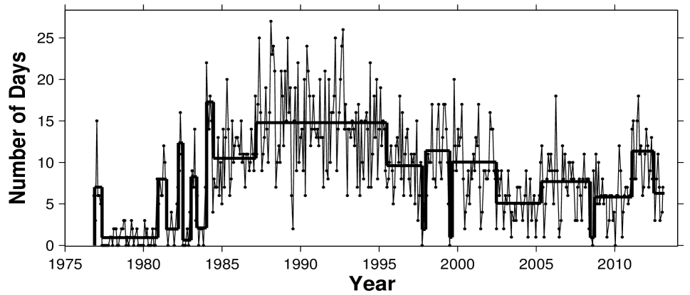
The mean interval between samples was 3.39 days, and the median interval exactly 1 day.

We here report exploratory analysis of these time series data, aimed at characterizing the variability of the individual parameters in a number of ways, and to investigate possible relationships between them. For background the reader may consult the review paper (, 2008) on stellar chromosphere activity. The book (, 2000) provides excellent overview of the relevant solar physics and stellar physics. The paper (, 2007) details analysis of McMath Solar Telescope data similar to those described here.

The following sections describe time domain, correlation, power spectrum, and time-frequency analyses carried out on these data. The emission index $\bf EM$ and core intensity $\bf K_{3}$ are emphasized, because these two closely related parameters vary in quite similar ways and seem to be the most straightforward diagnostics of chromospheric activity. No data preprocessing beyond that described in (, 1984) was applied, other than the removal of a few outliers.

2 The Time Series

Figure 2 presents these 3905 observations in the same format as Figure 2 of (, 1998), with the exception that the order is the same as listed above, and a few outlying points presumed to be erroneous have been replaced with linear interpolations. In addition an estimate of the $1\-\sigma$ observational error variance is plotted as a small vertical bar near the bottom of each panel just above the date 1980. These error bars are determined from an analysis of the auto-correlation function of the time series data, as described in §3. Note that these errors are quite small; the majority of even the apparently random variation is real and not due to observational errors.

Figure 2: Ca II K-line time series data, with a few outliers removed. Just above the date 1980 is a small bar representing the upper limit on the average error variance determined directly from the data as described in §3.

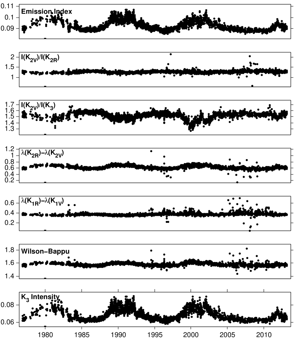
Figure 3 shows and enlarged version of the two intensity time series, EMDX and K3. The lines are fits to the data using the MatLab spline function spaps. The resulting smoothing has the effect of removing or reducing the shorter time-scale components, thus elucidating time-scales longer than a fraction of a year. Shown are fits with two different values for the spline error tolerance parameter. Roughly speaking the lesser smoothing reveals the solar cycle and the somewhat faster quasi-periodic variations to be discussed below, while the greater smoothing mostly removes the latter and emphasizes the former.

Figure 3: Time series of EMDX (top) and K3 (bottom), with spline fits computed with two different degrees of smoothing: greater smoothing as the dark line, less smoothing as the white-filled line.

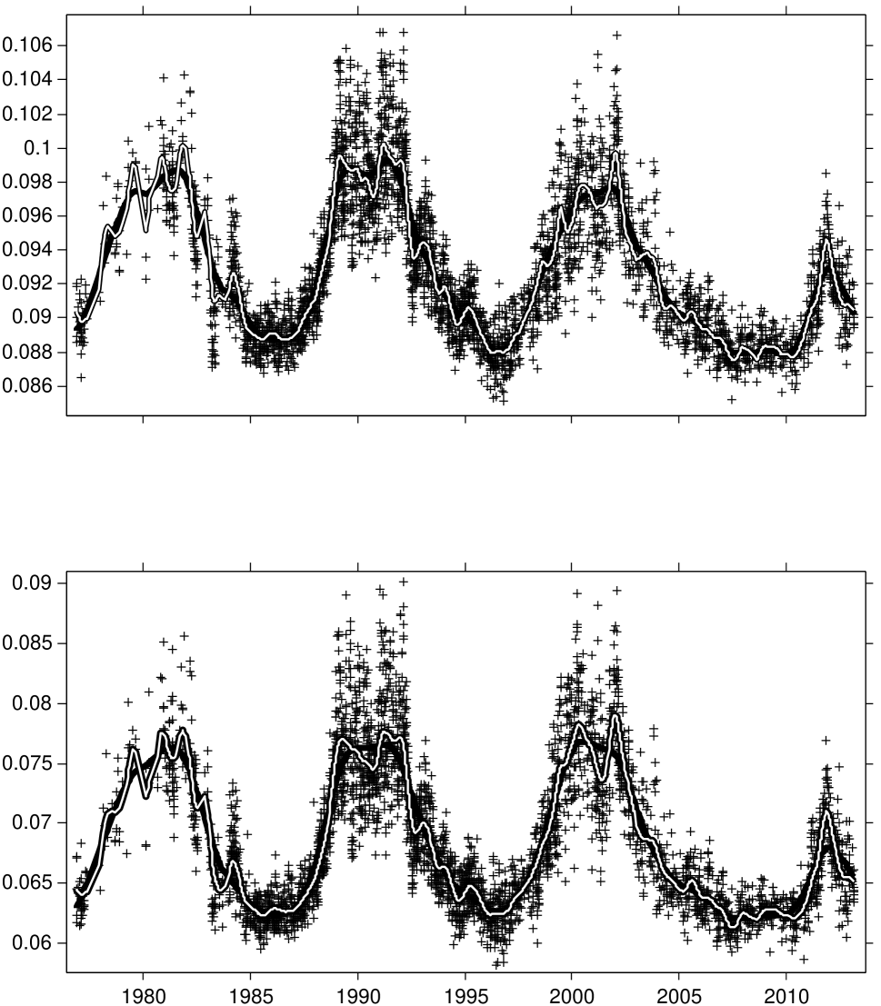
Figure 4 makes a side-by-side comparison of the two variables EMDX and K3, with both degrees of smoothing. Figures 3 and 4 between them make two points: (1) these two intensity variables, under either of the adopted smoothing choices, have very similar behavior; and (2) the more complex structure corresponding to the smaller degree of smoothing, while not identical, is similar over the three cycles. This first point is not unexpected because these variables measure similar aspects of the central depth of the K-line. The second point is perhaps surprising, as it suggests that the solar cycle as seen in chromospheric activity is repeatably more complex than a series of simple monotonic rises to maximum followed by declines to minimum.

Figure 4: Direct comparison of the two variables ${\bf EM}$ (solid lines) and ${\bf K_{3}}$ (dashed lines). Shown are spline fits to the raw data with outliners removed: heavier smoothing in the top panel and less smoothing in the bottom one.

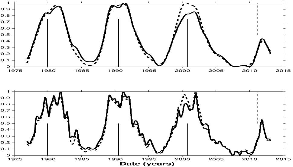
We regard the repeatability of the irregular structures in the plots in the bottom panel as evidence that they more correctly represent the true behaviors of these parameters over the solar cycle than do the smoother ones. (Note especially cycles 21 and 23: three sharp peaks near solar maximum, with similar peaks on both the rising and falling parts of each cycle.)

As will be detailed in this and the following three sections, there are four types of variability, plus observational errors, present in all of the time series: (a) a periodic trend obviously tied to the 11-year solar cycle, (b) quasi-periodic signals an order of magnitude faster than (a), (c) random flicker noise, (d) a periodic signal at or about the solar surface rotation frequency, and (e) the inevitable errors of observation.

Figure 5: A short segment of the EMDX light-curve near the peak of cycle 22. The vertical dotted lines are separated by the period corresponding to the peak of the power spectrum of the data in this 3.4-year long interval. (Accordingly this period, 26.49 days, has meaning only for this limited time window.) The solid bar in the middle/top part of the figure is the $1\sigma$ observational error variance determined in §3.

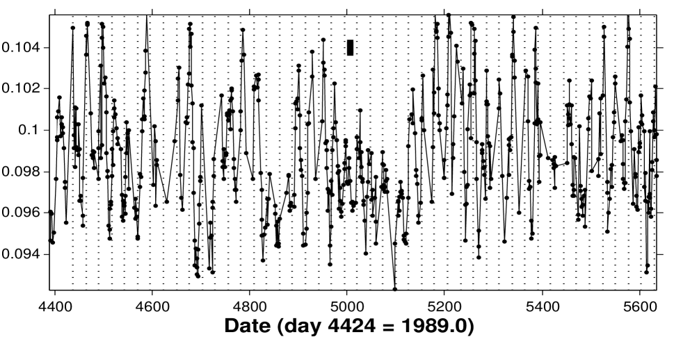
The first two of these are the relatively smooth variations just discussed. The third and forth are difficult to distinguish from each other visually in light curves. However the major part of the variability in the magnified plot in Figure 5 is rotational modulation. While there is not a precise one-to-one correspondence between peaks and the fiducial lines at the solar rotation cadence, the presence of a periodicity with an amplitude well above the observational errors is strongly suggested. In §4 and §5 all of these variation components (a)-(e) are separated from each other using power spectrum and time-frequency analysis of the residuals obtained by subtracting a smoothed fit from the raw data. While this phenomenological separation may not mean that there really are four independent components, all of them are clearly real and originate from chromospheric activity, or a modulation thereof in case (d). The observational errors are small, as demonstrated in §3. In addition the details of the variation of EMDX and K3 are much the same (see Figure 4), which would not be the case if observational errors were significantly large. It is difficult a priori to rigorously identify the physical processes underlying these components, but the properties listed in Table 1 argue for distinct physical origins of the components.

Table 1: Five Modes of Variability

	Amplitude	Time-Scale	Nature
(a) Solar cycle	large	long ($\approx$11 years)	deterministic
(b) Rieger-type periods	small	medium ( $\approx$ 100 days)	quasi-periodic
(c) Flicker noise	small	large range	random
(d) Rotation modulation	medium	short (27 days)	periodic
(e) Observation errors	small	instantaneous	random

A positive amplitude-variance correlation is clearly evident in the EMDX and K3 time series, and less prominently the others: variance large near the peaks and small near the valleys. The plot of the residuals from a smooth fit in Figure 6 makes this effect even more obvious.

Figure 6: Residuals of the EMDX data from the adopted smooth fit; this fit is plotted at the bottom with an arbitrary offset and scaled down by a factor of 2 realtive to the residuals.

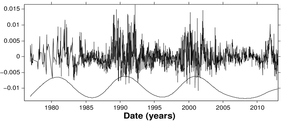
Such correlations are expected, in view of the large contribution to the variance from rotationally modulated chromospheric activity (cf. Fig. 5) closely following the solar cycle.

Figure 7: Scatter plots of (a) EMDX residuals and (b) variance of these residuals, vs. the smoothed EMDX  parameter are binned in a 32x32 grid of 2D bins and displayed as grey scale images. The superimposed white lines are (a) zero residual and (b) a least squares regression line.

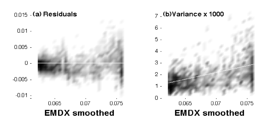
Figure 7 is another way to visualize the relationship between the random and smoothed EMDX. By construction the residuals average to zero, as in (a). The increase of the variance with amplitude is explicit in (b) and supported by the increase of the range of the residuals with emission in (a).

The following Table 2 presents summary statistics for the seven variables. Except for the error estimates described in §3 these were all computed in straightforward ways directly from the time series data. The first three rows (after one specifying the units for the quantity) contain the mean, range, and standard deviation computed directly from the raw observations with outliers removed. Row four is the standard deviation of the residuals from the adopted smooth fit to the relevant time series. Row five gives the estimated RMS observational errors described in the next section; these should be taken as upper limits for reasons described there. Row six is the relative error obtained by dividing row five by row two. Row 7 is the index $\alpha$ in power-law fits ($P(f)\sim f^{\alpha}$) to the power spectra, described in §4.

Table 2: Statistics of the K-Line Time Series

	EMDX	VIORED	K2VK3	DELK1	DELK2	DELWB	K3
Units	Eq W	$\Delta$ intensity ratio	intensity ratio	$\Delta$Å	$\Delta$Å	$\Delta$Å	intensity
Mean	0.0929	1.2700	1.5146	0.6304	0.3748	1.5832	0.0687
Range	0.0129	0.2256	0.2648	0.1862	0.0918	0.1031	0.0211
$\sigma$	0.0043	0.0444	0.0549	0.0508	0.0204	0.0212	0.0062
Residual $\sigma$	0.0018	0.0321	0.0250	0.0229	0.0144	0.0116	0.0024
Error $\leq$	0.0005	0.0303	0.0133	0.0180	0.0114	0.0108	0.0006
Error / Range	0.0423	0.1343	0.0501	0.0967	0.1241	0.1052	0.0290
$\alpha$	-0.303	0.004	-0.175	-0.108	-0.114	-0.009	-0.238

3 Autocorrelation Analysis

An autocorrelation function contains information about the memory of the underlying process, be it random or deterministic. This function elucidates connections between the quantity at different times; specifically the autocorrelation function $\rho(\tau)$ characterizes the joint variability at times $t$ and $t+\tau$ averaged over $t$. (In the next section we will also use the autocorrelation as a handy way to compute power spectra and time-frequency distributions.)

The panels of Figure 8 exhibit the rather complex multi-scale behavior of the auto-correlation function for EMDX – computed using the Edelson and Krolik algorithm (, 1988) as described in Appendix 2 – emphasizing three important time scales. The first panel shows the autocorrelation function (normalized to unity at zero lag) extending to the maximum lag, namely the 12671 day length of the time series, thus emphasizing time scales $\approx$ the solar cycle. The bottom two panels plot the unnormalized autocovariance function (different by only a constant factor, and indicating actual variances) covering: lags in the range of the surface rotation period, and the smallest times scales corresponding to the one-day sampling of the raw data, respectively.

The overall behavior of the autocorrelation is dominated by variability at the frequencies of the solar cycle and the surface rotation. In the top panel much of the scatter about what would otherwise be a smooth function is due to a combination of several of the variability modes listed in Table 1: the stochastic signal (c), the rotational modulation (d), with a minor contribution of the errors (e). The increased scatter for large lags (only shown in the top panel) is simply due to the fact that for lags comparable to the length of the observation interval many fewer data points contribute to the average in Equation (4) of Appendix 2.

Figure 8: Edelson and Krolik correlation function of EMDX time series, with zero lag indicated by vertical dotted line. Top: Autocorrelation (normalized at zero lag) over the full range of lags. Bottom: unnormalized autocovariance at lags up to 64 days (left) and 7 days (right). Lags of multiples of 11 years (top) and the Carrington period of 27.2753 days (bottom) are shown as dashed vertical lines.

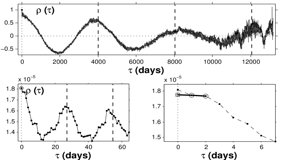
In the bottom right panel of Fig. 8 as one considers smaller and smaller lags the autocorrelation levels out somewhat at two days and one day, and the value at zero lag is notably higher than this level. This offset, also visible in the other panels, reflects the variance of the observational errors and provides a way to estimate the average observational error in the data. The auto-correlation function at zero lag is the sum of two contributions: the observational error variance and the true variance of the source. At any other lag the errors average to zero as long as they are uncorrelated. These remarks yield a procedure for estimating the size of the average observational error by attributing it to the excess contained in the zero-lag spike. Assuming the true autocorrelation function is reasonably smooth, the difference between an extrapolation to zero lag and the actual value $\rho(0)$ yields the variance corresponding to the observational errors. In the bottom-right panel of Figure 8 a linear fit to the autocorrelation at the first two positive lags (shown as circles) was extrapolated to the point contained in a square. For all seven parameters this difference between the actual and extrapolated zero-lag values is the error variance reported in Table 2.

Actually these should be taken as upper limits on the true error variance. Any solar variability confined to time-scales shorter than the sampling interval would make a contribution to the zero-lag spike that would be lost in our extrapolation procedure. Although known turbulence and oscillations likely contribute in this way, absent more quantitative information on how smooth the true autocorrelation function is on the diurnal time scale, the errors listed in Table 2 are probably reasonably good estimates.

4 Power Spectrum Analysis

Rotation can produce a periodic modulation of any solar time series. This signal might be expected to be relatively weak in full-disk observations of chromospheric lines, as discussed further in the next section, §5. Nevertheless one goal of this work is to detect and characterize any signatures of rotational modulation in the K-line time series. This section demonstrates the rather strong rotational signal present in these data and already remarked upon in §2 in connection with Figure 5. Rotation yields peaks in the power spectrum at the solar rotation frequency and its harmonics. Indeed even the more subtle effects of differential rotation can be studied in considerable detail, as shown in the following section.

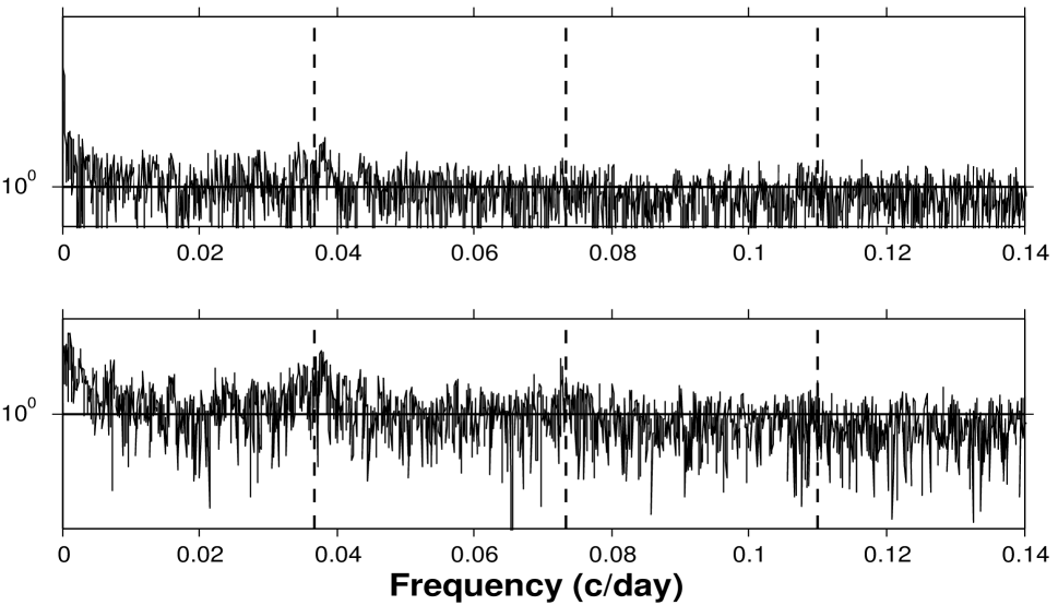
Figure 9 shows two power spectra for the EMDX time series, both computed using the Lomb-Scargle periodogram (, 1982). Power spectra computed from the Edelson and Krolik auto-correlation function, as mentioned in §3 and detailed in Appendix 2, are essentially identical to those shown here. The comparison is between the spectrum of the raw data (top) and that of the residuals from the smooth fit (bottom). The modulation at the rotation frequency and its harmonics is here largely buried in the noise inherent in such unsmoothed power spectra. It is slightly more prominent in the power spectrum of the residual data in bottom panel.

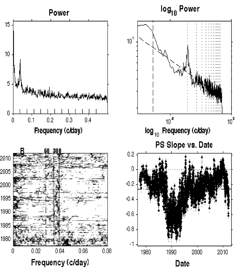
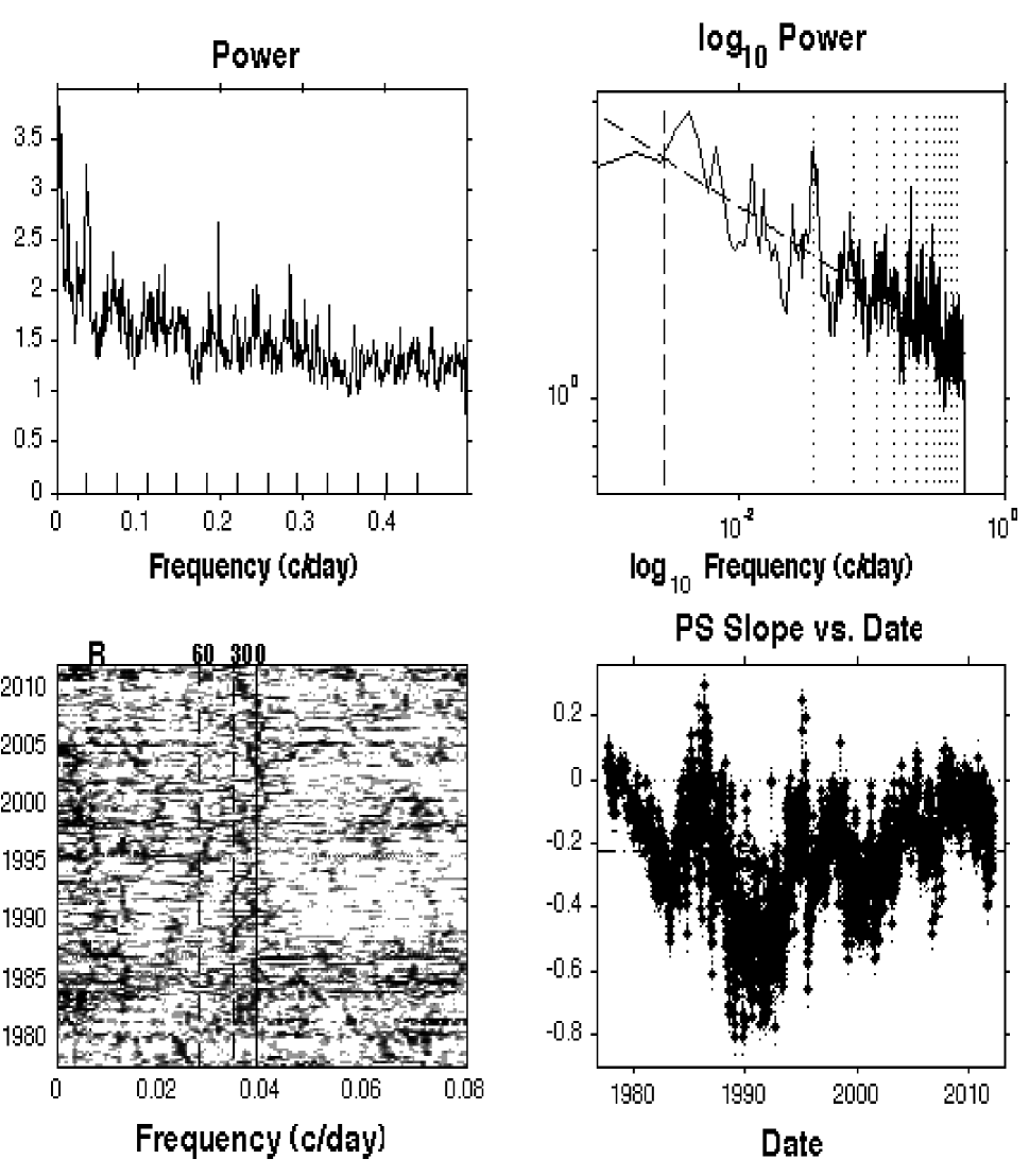
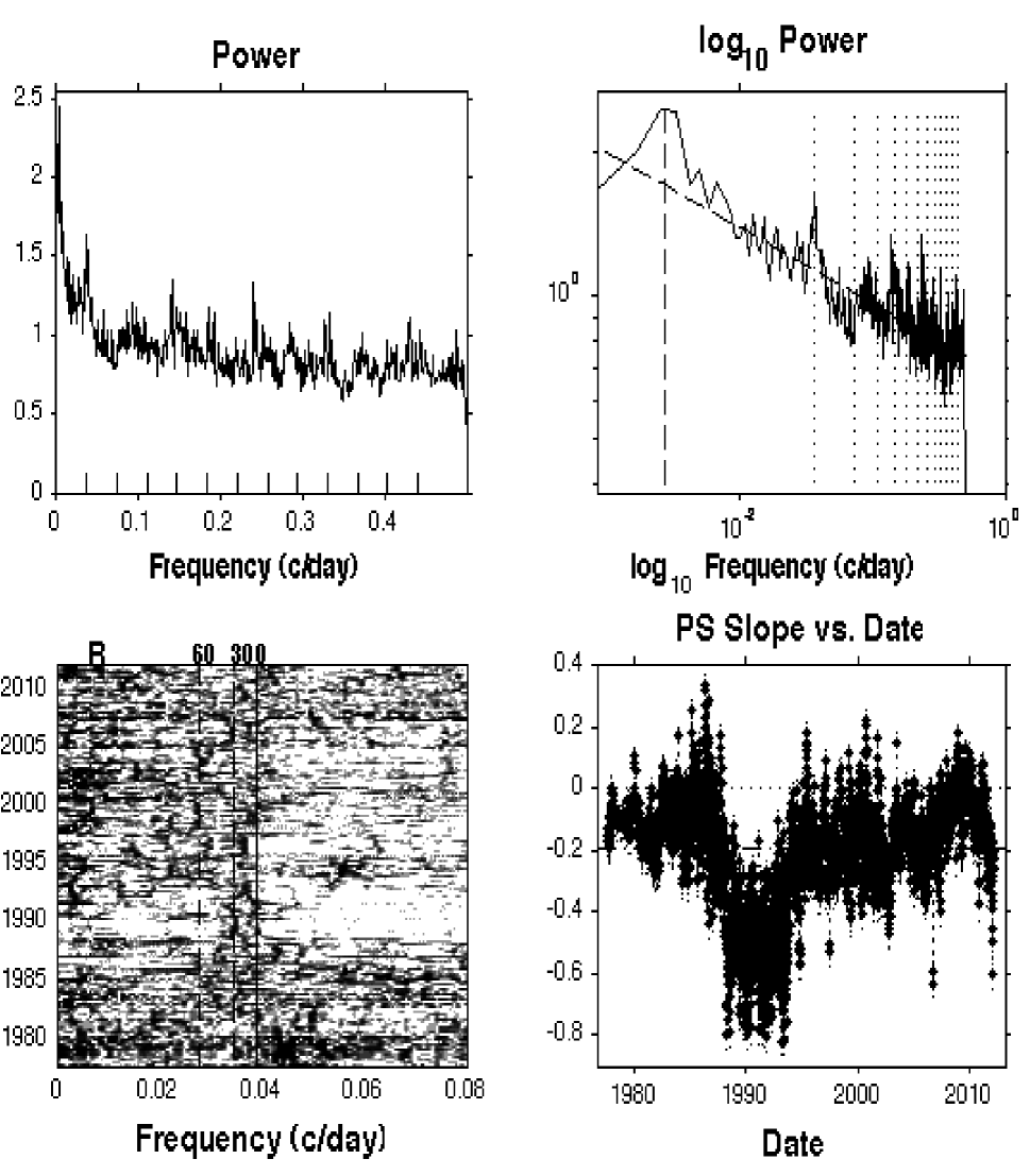
A feature of the power spectra of all seven parameters displayed in Appendix 1 is a component at all frequencies, most easily seen as an approximately linear trend in the log-log plots. That is to say the power varies approximately as $P(\nu)\approx\nu^{\alpha}$ with $\alpha$ taking on negative values between 0 and -1. Further $\alpha$ varies systematically with time (lower-right panels in Appendix 1). The most obvious feature of this variation is a steepening of the power law (less high frequency variability relative to that at lower frequencies) over a broad interval near the solar maximum of cycle 22 (1990-1992). This behavior is perhaps related to the fact that the overall activity in this cycle was stronger than in the other cycles, as can be seen in Figures 2 and 3, and the top panel of Figure 10 for example. Indeed the slightly less prominent high frequency background power for cycle 22 is perceptible in this panel.

Raw power spectra are typically noisy and require smoothing in order to fully reveal their information content. We do not pursue this avenue here, since an even more fruitful approach is detailed in the following section.

Figure 9: EMDX  power spectra, computed with the Lomb-Scargle periodogram, of: the raw EMDX data (top) and the residuals from smooth fit as shown in Figure 6 (bottom). Vertical dashed lines denote the nominal rotation frequency (corresponding to the Carrington period of 27.2753 days) and harmonics.

5 Time-Frequency Distributions

Rotation induces a harmonic variation of any signal from a localized region of the Sun’s surface and observed from a fixed direction. In the case of spots and active regions differential rotation modulates the observed period as they experience the latitude drift tied to the solar cycle. The summation of sources at various solar longitudes and latitudes inherent to full disk observations smears out the power spectrum and dilutes the signature of differential rotation. Nevertheless a surprising amount of information about the Sun’s rotation is contained in the full-disk K-line time series, as we shall now see.

The time-frequency distribution is designed specifically to explore this sort of evolving harmonic structure. In a nutshell this signal processing tool displays the time evolution of the power spectrum. The excellent treatise (, 1999) explains what can be learned with the basic tool and a number of its variants. Here we use the simplest approach, namely computing power spectra of the data within a sequence of time windows covering sub-intervals of the full observation span. Accordingly this tool is also called a dynamic or sliding window power spectrum. The output is a three dimensional data structure – power (z-axis) as a function of time and frequency (x- and y-axes) – that we here render as 2D grayscale plots.

A slice of this plot parallel to the frequency axis contains the power spectrum (power vs. frequency) at a specific time. A slice parallel to the time axis depicts the time dependence of power at a specific frequency. The same mathematics leading to the Heisenberg uncertainty principle dictates that these slices’ resolutions cannot both be made small independently: good frequency resolution can be had only with relatively large time windows, and good time resolution requires short windows. Any implementation of the time-frequency distribution allows one to mediate this unavoidable resolution trade-off, for example by adjusting the size of the window. A few further details of the computation of time-frequency distributions are given in Appendix 2.

Figure 10 shows time-frequency plots for the emission index. Because the data are not evenly spaced, all of the time-frequency distributions shown here were computed using the interpolation-free techniques described in Appendix 2. The cross symbols near the top right corners indicate the time and frequency resolution. The length of the arms of the cross indicate the width of the sliding window and the corresponding fundamental frequency. The solid, dashed, and dot-dashed vertical lines mark the frequency range corresponding to the rotation rate as a function of solar latitude, using Equation (3) of (, 1989):

$${\Omega_{p}\over 2\pi}=452-49\mu^{2}-84\mu^{4}\ \ \ \mbox{nHz}\ ,$$ (1)

labeled with the corresponding latitudes (in the $0$ to $60$ degree range normally inhabited by spots). The dotted line labeled “R” is the frequency corresponding to the Rieger period, taken as 155 days.

Figure 10: Time-Frequency distribution of EMDX residuals. Bottom, renormalized to make constant the power between the frequencies corresponding to 0 and 30 degrees, bringing out behavior during solar minimum that is otherwise lost. Vertical lines denote latitudes 0, 30, and 60 $\deg$ based on Eq. (1). The dotted line at .0082 c/d roughly corresponds to quasi-periodicities discussed in §4. Power below .00176 c/day is divided by 10 to improve the display.

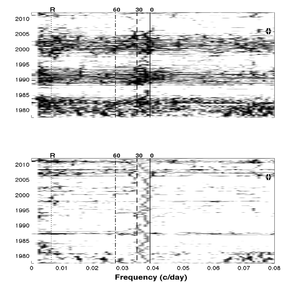
In the top panel of Figure 10 the rotational features almost disappear during solar minimum and are generally strongest in the middle cycle 22. It is instructive to adjust for these effects by renormalizing each time slice of the distribution. Note the interesting behavior of the rotational signal in the bottom panel, which is a renormalized version of the top panel. A relatively well-defined peak in power moves back and forth between approximately 0 degrees and 30 degrees latitude and is present essentially all of the time, not just during solar maximum as one might have concluded from the top panel.

The signal processing literature contains descriptions of many other ways to estimate time-frequency distributions (, 1999). One of the most recent ones, called synchrosqueezing, represents the time series as “the superposition of a (reasonably) small number of components, well separated in the time-frequency plane, each of which can be viewed as approximately harmonic locally, with slowly varying amplitudes” (, 2009). Figure 11 shows the result of this analysis for EMDX and K3 interpolated to even spacing, using the MatLab tools in (, 2009). The gray scale represents the power spectrum of the variables, as a function of time and frequency.

Figure 11: EMDX and K3  time-frequency distributions computed with the synchrosqueezing algorithm of Brevdo and Daubechies. The number-of-voices parameter = 50. The vertical lines represent the same nominal frequencies bracketing differential rotation as in Figure 10.

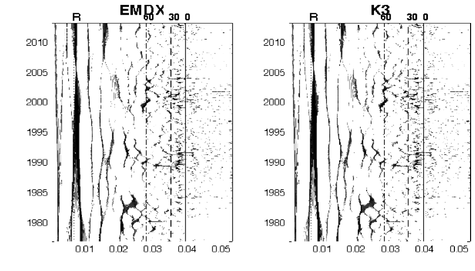
There are broad similarities to the distributions in the previous figure, and the clear differences in detail can be understood in terms of the constraints imposed by the synchrosqueezing method on the time-frequency atoms, as well as the fact that interpolation to even spacing was necessary. The more fully non-parametric sliding-window Fourier power spectrum spectrum yields a different representation of the underlying time-frequency structure. The synchrosqueezing algorithm renders the differential rotation features as more discrete than does the sliding-window approach; the reverse is true of the quasi-periodic signals with periods in the vicinity of 0.002-0.015 cycles per day.

6 Cross- Analysis

Each of the seven K-line parameters probes a different aspect of the chromosphere. Therefore relations between the corresponding time series can elucidate physical processes driving the underlying activity. For example variability in two parameters that is correlated, anti-correlated, or correlated with time-lags can shed light on underlying dynamical processes. Of course causality cannot be proven in this way, but relationships consistent with physical models can be elucidated.

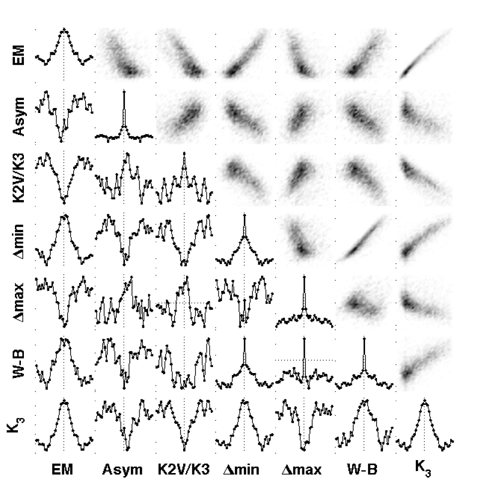
Figure 12 depicts two types of cross-analytic relationships for all pairs of parameters. The 21 scatter plots above the diagonal describe pairwise mutual dependence. Below and on the diagonal are cross- and auto-correlation functions, respectively; all were computed with the Edelson and Krolik algorithm (cf. §3 and Appendix 2).

These types of displays are complementary ways of relating two variables. Independence is a stronger statistical condition on two variables than their being uncorrelated. The former implies the latter, but not vice versa. Hence to the extent that scatter plots elucidate dependence they are more powerful statistically. However they depict only simultaneous relationships, whereas cross-correlation functions elucidate how the variables at two different times are related.

Figure 12: Diagonal: Auto-correlations. Above Diagonal: Scatter plots. Below Diagonal: Cross correlations. All correlations are for $|\tau|$ $\leq 20$ days. In computing the quantities displayed in this figure all seven parameters (with outliers removed) were standardized to zero mean and unit variance.

7 Wilson-Bappu Effect

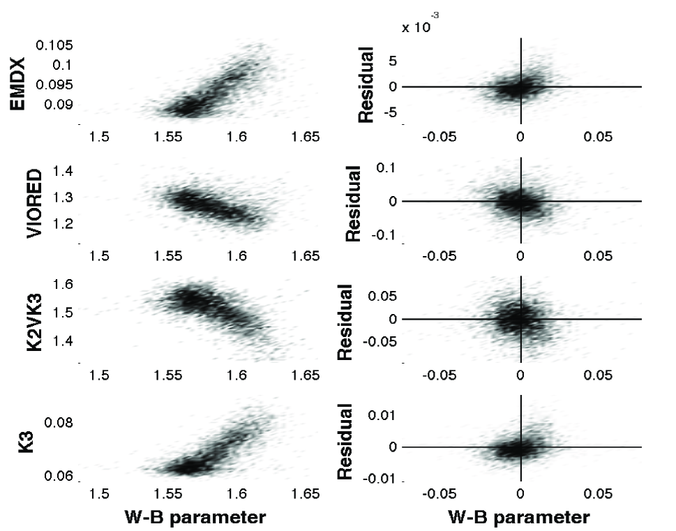
In these data there is evidence for a Wilson-Bappu effect in the sense that the intensity parameters correlate with the width of the K-line. Figure 13 contains scatter plots for the four intensity parameters vs. the Wilson-Bappu parameter, presented as $64$ by $64$ two-dimensional histograms portrayed as greyscale plots. The left-hand column contains scatter plots for the raw data (with outliers removed). These correlations are presumably due to chromospheric processes tied to the variations in physical conditions over the solar cycle. The right-hand column shows the corresponding residuals from the smooth fits described in §2, which are essentially uncorrelated.

Figure 13: Intensity variables vs. Wilson Bappu parameter. Left-hand column: raw measurements (with outliers removed). Right-hand column: residuals

8 Conclusions

This is basically an exploratory study of the data collected in the K-line monitoring program. The main goal is to follow the clues provided by various time series analysis methods in the time-, lag-, frequency- and time-scale domains, rather than to validate specific astrophysical hypotheses.

Affecting the interpretation of any results is their significance in light of random observational errors and systematic errors. Even though point-by-point errors are not available, in §3 we have placed reasonable upper limits on the average error variance. In addition, it is difficult to construct and display errors on 2D and especially 3D functions such as time-frequency distrbutions. We rely on comparison of the various functions to indicate the rough importance of observational errors. For example the time-frequency distributions for EMDX and K3 for the most part show the same beavior and therefore indicate that such errors are not large. The other parameters show signficantly different behavior, but comparison of similar ones (such as the three wavelength differences) gives a similar indication of the signficance of the time-frequency structures.

In §2 we presented evidence for a relatively complex structure to the solar cycle, somewhat different from the standard concepts of the sunspot cycle and other heliospheric phenomena discussed by a number of authors. Apparently the K-line features are particularly sensitive to the changing physical conditions during the solar cycle. A carefully chosen degree of smoothing of the time series is essential to elucidating this structure.

The basic notion of complexity in the solar cycle is not new, although previous work has centered mainly on a relatively simple “double peak” concept in sunspot and other heliospheric indices at the time of solar maximum. For example, in yearly averages of the number of intense geomagnetic storms (, 1990) describes time series behavior that generally follows the solar cycle, but with a double peak structure: “ … one at the late ascending phase of the cycle and another at the early descending phase,” with hints of even more complex three-peaked structure for cycle 20. In (, 2010) Figures 16 and 38 show distinct double peak structures in the smoothed International Sunspot Number, and Figure 42 shows the same for the Polar Magnetic Field Strength as measured at the Wilcox Solar Observatory. One presumes that the weakness of apparent double peaks in sunspot number averaged over cycles 1 to 22 depicted in that paper could be because of slight variations of the times of the peaks as well as the degree of smoothing applied to the individual curves. Figure 9 in (, 2009) depicts a double peak and more complex structure in the time series for sunspot numbers, 10.7 cm. radio flux, a Ca K 1 $\AA$ full-disk index from Kitt Peak, and a Mg II index. The reference (, 2002) gives an overview of structure in sunspot variability on various time scales, referring to the kind of structure noted here as “quasi-biennial oscillations.” The complex time series structures shown in the bottom panel of our Figure 4 perhaps correspond to multiple toroidal field surges as discussed by (, 2011).

A somewhat related issue is the structure noted in the time frequency distributions, possibly connected to the solar cycle but at frequencies lower than those due to surface rotation. There is discussion in the literature of such frequencies, often in the context of an early claim of a 154 day periodicity in solar gamma-ray flares (, 1984), which was followed by attempts to find similar periods in other phenomena. (, 1996) discusses an idea in which a more complex structure consisting of multiples of a fundamental period of approximately 25.5 days underlies the Rieger periodicity; see also (, 1993, 2013). (, 2009) discusses a period of 151 days in solar cosmic ray fluxes. (, 2005) find a 123-day period in soft x-ray flux from the sun, and (, 2003) find a very similar period (and others) in solar coronal mass ejections. The relevance of similar periodicities occurring in other stars (, 2005) is unclear.

The K-line data as analyzed in the time-frequency distributions in §5 suggest the presence of some quasi-periodic behavior on similar time scales. We found that peaks in a sine wave of suitably chosen period and phase matches many of the peaks in the partially smoothed EMDX time series. A period of 122.4 days was obtained in a rough peak-fitting procedure. However, keeping in mind the degrees of freedom in the sinusoid, the uncertainty in locating and timing the peaks in the data, and the matching of some peaks and not others, this result does not prove the existence of a pure harmonic signal. Rather as indicated in the time-frequency distributions there appears to be quasiperiodic behavior in this frequency range.

Another result of our analysis is the characterization of differential surface rotation, using the time-frequency tool, as described in §5 for the main intensity variables, with displays for all of the variables in Appendix 1. For discussions of differential rotation estimated from time series from Kepler and CoRoT see (, 2011) and (, 2011) respectively.

Here is a summary of our broad conclusions:

• The solar cycle variability [component (a) in Table 1] of the K-line intensity consists of the well-known broad oscillation paralleling the 11-year sunspot cycle.

• In addition there are quasi-periodic oscillations that do not have constant periods or amplitudes, but irregularly populate the time-frequency domain in the neighborhood of periods of roughly 100 days. It is not clear if these are modulations of the solar cycle or a physical process independent of same.

• The random variations [”Flicker noise”; component (c) in Table 1] in all seven parameters have power spectra describable as “${1\over f}$ noise,” meaning $P(\nu)\approx\nu^{\alpha}$. The index $\alpha$ is always negative and exhibits systematic variations over time apparently correlated with the general level of chromospheric activity. Perhaps higher activity is due to many individual independent fluctuations, the summation of which effectively smoothes higher frequency variations as a purely statistical effect. Or some other inherent feature of the randomness of the underlying physical process may suppress rapid dips from states of higher to lower activity.

• Components (a) and (b) are, roughly speaking, independent of each other, except that the variance of (b) is correlated with (a) [Figures 6 and 7].

• A signature of differential surface rotation is captured by time-frequency analysis of especially the EMDX time series. While this behavior roughly mirrors the general character the butterfly diagram for sunspots, in detail it is distinctly different. These differential rotational signatures of the K-line parameters continue during solar minimum.

These conclusions refer mainly to the the parameters EMDX and K3, but to some degree apply also to others of the measured parameters.

Acknowledgements: We are grateful to Alexander Kosovichev, Kira Rehfeld and Luca Bertello for helpful comments, and to Joe Bredekamp and the NASA Applied Information Systems Research Program for encouragement and support. The observations used herein were obtained at the Evans Solar Facility of the National Solar Observatory. We are grateful for the assistance of NSO personnel, especially John Cornett, Timothy Henry and Lou Gilliam for observing and reduction of the raw data to produce the Ca II K-line data archive. The NSO is operated by the Association of Universities for Research in Astronomy, Inc. (AURA), for the National Science Foundation.

Appendix 1: Power Spectra and Time-Frequency Distributions

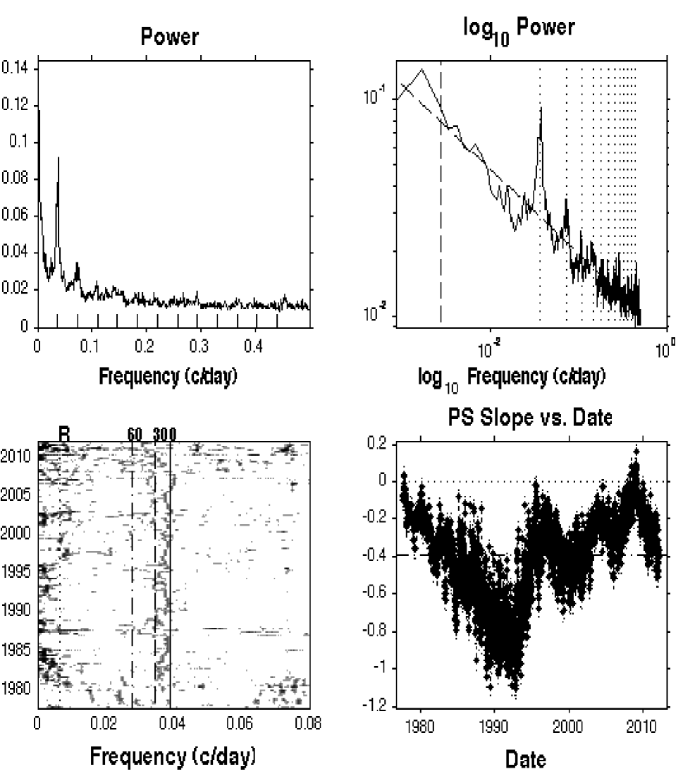
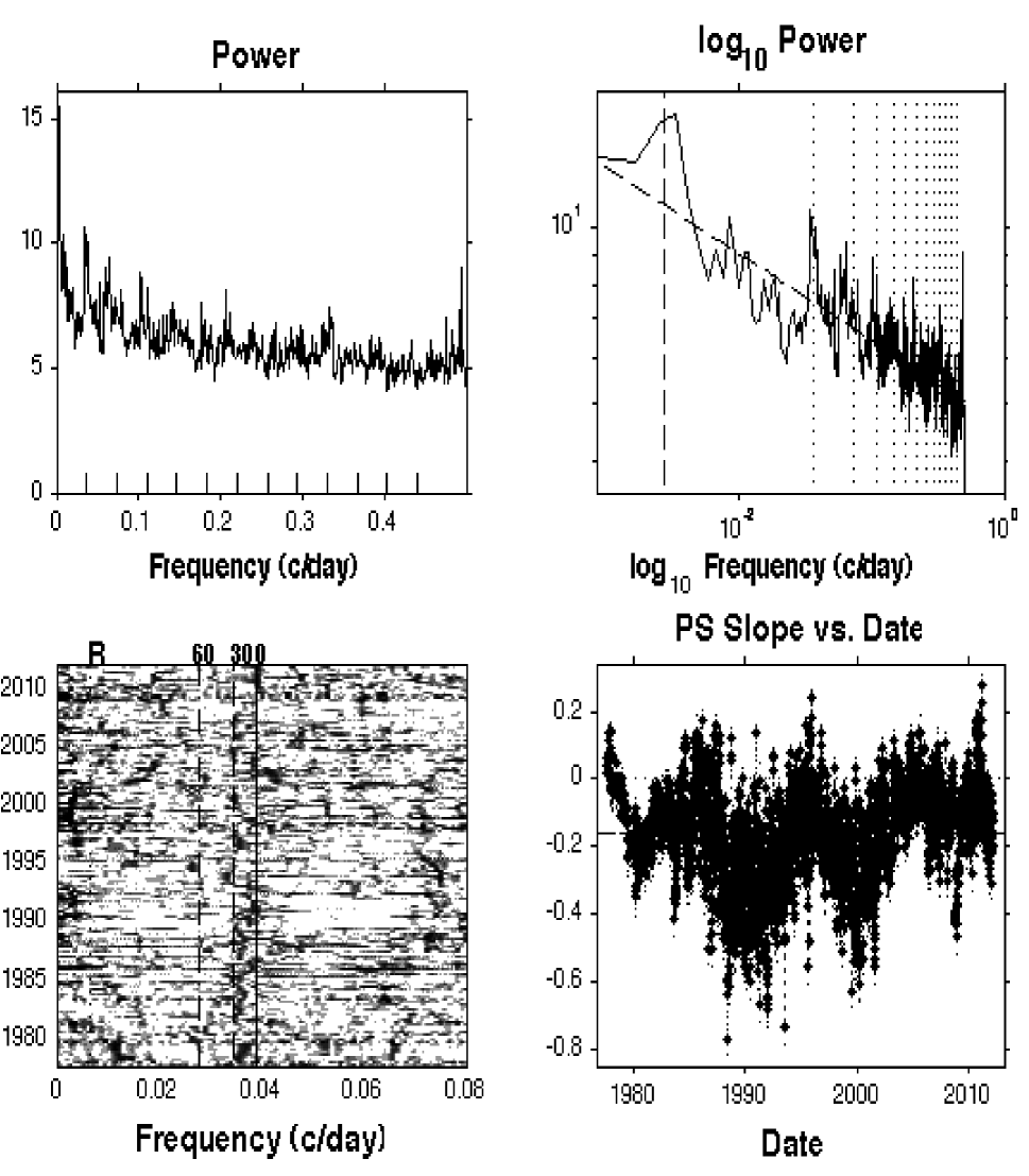
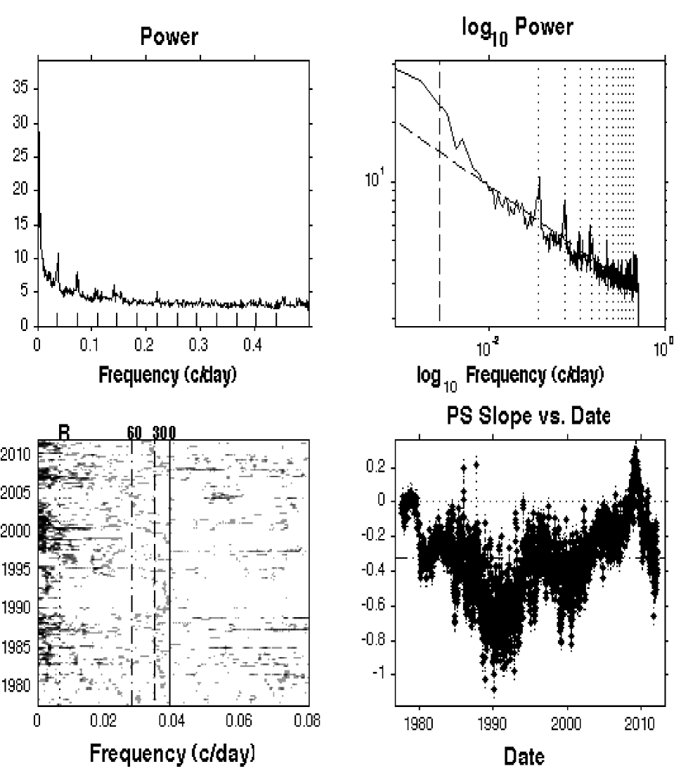
This appendix presents power spectrum analysis of all of the measured variables. In each of the seven figures the top two panels show the Edelson and Krolik based power spectra of the residual time series, plotted linearly (left) and doubly logarithmically (right). A ${1\over f}$ power spectrum corresponds to a straight line in the latter; a dashed line shows the corresponding least-squares fit excluding the regions of the rotational peaks. Vertical lines indicate frequencies corresponding to a 27.2753-day nominal surface rotation period (the Carrington period) and its harmonics. The vertical dashed line in the upper right panel marks a fiducial frequency corresponding to a period of one year. The 11-year frequency is too small to plot effectively here.

The lower-left panel shows the time-frequency distribution obtained by computing the power spectrum in a time-window slid along the time series. These were normalized much as in the bottom panel of Fig. 10, but over the broader frequency range 0.02-0.04 cycles/day. The power spectra shown in the top two panels were obtained by averaging this time-frequency distribution over the time coordinate. Accordingly they are considerably smoother than would be obtained directly from the time series. The upper-right panel shows the full frequency range extending to the Nyquist frequency (${1\over 2}$ cycle/day), but in both of the left-hand panels only a restricted range covering the most interesting behavior is plotted.

The bottom-right panel shows the temporal variation of the slope of the power-law fit to the power-spectrum – that is the value of $\alpha$ in a representation of the form

$$P(f)=P_{0}f^{\alpha}\ .$$ (2)

Note: we adhere to the convention that a process that even approximately satisfies this equation with any value of $\alpha$ (almost always negative) is called “${1\over f}$ noise”. Comments on the systematic variation of this parameter are contained in Section 8.

Figure 14: Power spectra (with power-law fits) and time-frequency distributions of EMDX.

Figure 15: Power spectra (with power-law fits) and time-frequency distributions of VIORED.

Figure 16: Power spectra (with power-law fits) and time-frequency distributions of K2VK3.

Figure 17: Power spectra (with power-law fits) and time-frequency distributions of DELK1.

Figure 18: Power spectra (with power-law fits) and time-frequency distributions of DELK2.

Figure 19: Power spectra (with power-law fits) and time-frequency distributions of DELWB.

Figure 20: Power spectra (with power-law fits) and time-frequency distributions of K3.

Appendix 2: Notes on the Computations

These time series represent a special case of irregular sampling, namely evenly spaced (at 1-day intervals) but with some missing observations. The degree of departure from even sampling is depicted in Figure 21.

Figure 21: Distribution of data gaps: Logarithm (base 10) of the number vs. interval size. For clarity this histogram omits nine large gaps (62, 70, 71, 82, 83, 123, 130, 216 and 174 days) from the early years of the program (before 1982.5). The spike of one-day intervals (2125 out of 3732, or 57 per cent ) refers to the nominal daily sampling; anything larger is a gap.

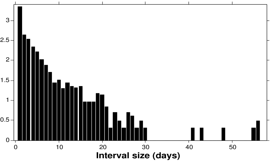
Because of the non-trivial number of gaps and the wide distribution of their sizes it is necessary to compute correlation functions and power spectra with methods that account for uneven sampling. For direct computation of frequency domain quantities (e.g. Fourier transforms, phase and power spectra) the Lomb-Scargle Periodogram (, 1971, 1975, 1976, 1982, 1989) is used here, and has been previously used to study this very data (, 1995). This appendix describes the computation of correlation functions for arbitrarily spaced data for their own sakes as well as as an alternative route to frequency domain quantities.

These computations start with the correlation algorithm (, 1988) often used in astronomy and well studied in the signal processing literature, under the name of slotted techniques – see e.g. (, 2006, 2011). It is an effective way to estimate the auto-correlation function for unevenly spaced time series data $x(t_{n})$ such as we have here. The basic idea is to construct bins in the lag variable $\tau$, and then sum the product $x(t_{1})x(t_{2})$ over all data pairs such that the difference $t_{1}-t_{2}$ lies in a given such bin:

$$\tau_{k}\leq t_{1}-t_{2}\leq\tau_{k}+\Delta\tau\ ,$$ (3)

where $\tau_{k}$ denotes the start of bin $k$ and $\Delta\tau$ is the bin width. That is to say the autocorrelation estimate is

$$\rho(\tau_{k})={1\over N_{k}}\sum_{n}x_{n}x_{m}\ ,$$ (4)

where the sum is over all pairs $n,m$ such that the corresponding time difference $t_{n}-t_{m}$ lies within the bin defined in Eq. (3), and $N_{k}$ is the number of terms in the sum. It is more usual to write this formula replacing $x_{n}$ with $x_{n}-\mu_{x}$, where $\mu_{x}$ is the mean value of $x$, either theoretical or empirical. Here we assume an empirical mean has been subtracted. The basic idea is that the average product $x(t_{1})x(t_{2})$ describes the degree to which values separated by $\tau$ are related (large if positively correlated, large and negative if anti-correlated, and small if uncorrelated).

The role of the factor ${1/N_{k}}$ is interesting. In estimating correlation functions for evenly spaced data two variants are used

$$\rho(k)={1\over N}\sum_{n}X_{n}X_{n+k}\\$$ (5)

and

$$\rho(k)={1\over N-k}\sum_{n}X_{n}X_{n+k}$$ (6)

representing a trade-off favoring small variance (with larger bias) or unbiased (but with larger variance) respectively. Equation (4) corresponds to equation (6) in that in both cases the denominator in the prefactor is the number of terms contributing to that value of the lag, so the expression is truly an average. If desired the analog of Equation (5) could be implemented in an obvious way.

Even though Equation (4) seems a bit abstract it is easily computed in practice. For evenly spaced data with gaps the binning in $\tau$ should correspond to the constant sampling interval. The power spectrum can then be computed using the well-known identity that the power spectrum is the Fourier transform of the autocorrelation function (which needs to be evaluated to the maximum lag possible, namely equal to the entire time-span of the observations). With even spacing of the lag variable this transformation can be rapidly carried out using the fast Fourier transform. One potential difficulty is the possibility that the sampling and choice of binning in $\tau$ yields some empty bins – no terms in Equation (4) that satisfy Equation (3). With the sampling in the present case (and with $\Delta\tau=1$ day) there are no empty bins. In addition the power computed in this way can be negative, since the autocorrelation may lack the properties that guarantee a non-negative Fourier transform. In practice this is a small effect ameliorated simply by taking the absolute value.

With an algorithm in hand to compute the power spectrum (either the procedure just outlined or the Lomb-Scargle periodogram) it is completely straightforward to compute the time-frequency distribution simply by accumulating a matrix of power spectra of the data points in a sequence of windows slid along the observation interval. The most important parameter is the width of the window. A good choice with the present data was found to be about 0.05 times the whole interval, or about 1.8 years.

References

- (1) Bai, T. and Sturrock, P. 1993, ApJ, 409, 476.
-
(2)
Brevdo 2009,
MatLab toolbox for Synchrosqueezing:
http://www.math.princeton.edu/~ebrevdo/synsq/. - (3) Brown, T. M., Christensen-Dalsgaard, J., Dziembowski, W. A., Goode, P., Gough, D. O., Morrow, C. A. 1989, ApJ, 343, 526-546.
- (4) Daubechies, I., Lu, J. and Wu, H.-T. 2011, Applied and Computational Harmonic Analysis, 30, 2011, 243
- (5) Domingo, V., G Ermolli, I., Fox, P., Haberreiter, M., Krivova, N., Kopp, G., Schmutz, W., Solanki, S. K., Spruit, H. C., Unruh,m Y., and Vögler 2009, Space Sci. Rev., 145, 337
- (6) Donohue, R., and Keil, S. 1995, Solar Physics, 159, 53
- (7) Edelson, R. A. and Krolik, J. H. 1988, Astrophysical Journal, 333, 646
- (8) Flandrin, P., Time-Frequency/Time-Scale Analysis (In French: Temps-Fr quence) 1999, Academic Press: London
- (9) Frasca, A., Fr hlich, H.-E., Bonanno, A., Catanzaro, G., Biazzo, K. and Molenda- Zakowicz, J. 2011, Astronomy and Astrophysics, 532, A81
- (10) Georgieva, K., “Why the Sunspot Cycle is Double Peaked,” ISRN Astronomy and Astrophysics (2011), Article ID 437838 arXiv:1103.4552
- (11) Gonzalez, W., Gonzalez, A., and Tsurutani, B. 1990, Planetary and Space Science, 38, 181-187.
- (12) Gottlieb, E. W., Wright, E. W. and Liller, W. 1975, Astrophysical Journal Letters, 195, L33
(13)
Hall, J. C. 2008,
Stellar Chromospheric Activity. Living Reviews in Solar Physics, 5, 2-+. Retrieved from
http://adsabs.harvard.edu/cgi-bin/nph-bib_query?bibcode=2008LRSP....5....2H -
(14)
Hathaway, D. 2010,
“The Solar Cycle,”
Living Rev. Solar Phys.,
7, 1.
http://www.livingreviews.org/lrsp-2010-1 - (15) Hill, M., Hamilton, D., and Krimigis, S. 2009, Journal of Geophysical Research, 106, 8315-8322.
- (16) Rachel Howe, “Solar Interior Rotation and its Variation,” Living Rev. Solar Phys. 6, 2009, 1. http://www.livingreviews.org/lrsp-2009-1
- (17) Jackson, B., Scargle, J.D., Barnes, D., Arabhi, S., Alt, A., Gioumousis, P., Gwin, E., Sangtrakulcharoen, P., Tan, L., and Tun Tao Tsai, 2005, IEEE Signal Processing Letters, 12, 105- 108
- (18) Joshi, B., and Joshi, A. 2005, Solar Physics, 226, 153-161.
(19)
Ca II K-line Monitoring Program,
Keil, S., Henry, T., White, D., and Livingston, B.,
http://nsosp.nso.edu/data/cak.pdf. This and other relevant documents, including the data analyzed in this paper, are available at the National Solar Observatory web sitehttp://nsosp.nso.edu/data/cak_mon.html, the data being atftp://ftp.nso.edu/idl/cak.parameters. - (20) Keil, S., Worden, S. P. 1984, ApJ, 276, 766
(21)
Keil, S., Henry, T., and Fleck, B. 1998,
NSO/AFRL/Sac Peak K-line
Monitoring Program,
Synoptic Solar Physics,
ASP Conference Series, 140,
Balasubramaniam, Harvey and Rabin, eds.,
also at
http://nsosp.nso.edu/data/cak_mon.html. - (22) Khramova, M., Kononovich, E., and Krasotkin, S. 2002, “Solar cyclicity: fine structure and forecasting,” in Solar variability: from core to outer frontiers. The 10th European Solar Physics Meeting, 9 - 14 September 2002, Prague, Czech Republic. Ed. A. Wilson. ESA SP-506, Vol. 1. Noordwijk: ESA Publications Division, ISBN 92-9092-816-6, 2002, p.145
- (23) Livingston, W., Wallace, L., White, O. R., and Giampapa, M. S. 2007, ApJ, 657, 1137
- (24) Lomb, N. R. 1976, Astrophysics and Space Science, 39, 447
- (25) Lou, Y., Wang, Y., Fan, Z., Wang, S., and Wang, J. 2003, MNRAS, 345, 809
- (26) Massi, M., Niedhöfer, Carpentier, Y., and Ros, E. 2005, A.&A, 435, L1
- (27) Percival, D. B. and Walden A. T. 1993, Spectral Analysis for Physical Applications: Multitaper and Conventional Univariate Techniques, Cambridge University Press, Cambridge, UK
- (28) Rehfeld, K., Marwan, N., Heitzig, J. and Kurths, J. 2011, Nonlinear Processes in Geophysics, 18, 389
- (29) Rieger, E., Share, G., Forrest, D., Kanbach, G., Reppin, C., and Chupp, E. (1984) Nature, 312, 623
- (30) Scargle, J. D. 1982, ApJ, 263, 835
- (31) Scargle, J. D. 1989, ApJ, 343, 874
- (32) Scargle, J., Norris, J., Jackson, B. and Chiang, J. 2013, ApJ, 764, 167
- (33) Schrijver, C. J. and Zwaan, C. 2000, Solar and Stellar Magnetic Activity, Cambridge University Press.
- (34) Silva-Valio, A., and Lanza, A. F. (2011), Astronomy and Astrophysics, 529, A36.
- (35) Stoica, P. and Sandgren, N. 2006, Digital Signal Processing, 16, 712.
(36)
Sturrock, P. 1996,
”A Conjecture Concerning the Rieger and Quasi-Biennial
Solar Periodicities,”
astro-ph/9609150 - (37) Sturrock, P., Bertello, L., Fischbach, E., Javorsek II, D., Jenkins, J. H., Kosovichev, A., and Parkhomov, A. G., 2013, Astroparticle Physics, 42, 62
- (38) Van ček, P. 1971, Astrophysics and Space Science, 12, 10
(39)
White, O., Livingston, W., Keil, S., and Henry, T.,
Variability of the Solar Ca II K Line over the 22 Year Hale Cycle
1998,
http://nsosp.nso.edu/data/cak_mon.html.