Nonlinear Color–Metallicity Relations of Globular Clusters. V. Nonlinear Absorption-line Index versus Metallicity Relations and Bimodal Index Distributions of M31 Globular Clusters

Abstract

Recent spectroscopy on the globular cluster (GC) system of M31 with unprecedented precision witnessed a clear bimodality in absorption-line index distributions of old GCs. Such division of extragalactic GCs, so far asserted mainly by photometric color bimodality, has been viewed as the presence of merely two distinct metallicity subgroups within individual galaxies and forms a critical backbone of various galaxy formation theories. Given that spectroscopy is a more detailed probe into stellar population than photometry, the discovery of index bimodality may point to the very existence of dual GC populations. However, here we show that the observed spectroscopic dichotomy of M31 GCs emerges due to the nonlinear nature of metallicity-to-index conversion and thus one does not necessarily have to invoke two separate GC subsystems. We take this as a close analogy to the recent view that metallicity–color nonlinearity is primarily responsible for observed GC color bimodality. We also demonstrate that the metallicity-sensitive magnesium line displays non-negligible metallicity–index nonlinearity and Balmer lines show rather strong nonlinearity. This gives rise to bimodal index distributions, which are routinely interpreted as bimodal metallicity distributions, not considering metallicity–index nonlinearity. Our findings give a new insight into the constitution of M31’s GC system, which could change much of the current thought on the formation of GC systems and their host galaxies.

1 INTRODUCTION

Systems of globular clusters (GCs) have long served the role of providing important constraints on theories of galaxy formation and assembly. GCs, which comprise stars with small internal dispersion in age and abundance, are always found in large galaxies and are easily identified out to large galactocentric distances due to their compact sizes and luminosities. A long-standing puzzle in the field of galaxy evolution is that GC systems exhibit bimodal color distributions (e.g., Geisler, Lee, & Kim, 1996; Kundu & Whitmore, 2001; Larsen et al., 2001; Peng, Ford, & Freeman, 2004; Harris et al., 2006; Peng et al., 2006; Lee et al., 2008a; Jordán et al., 2009; Sinnott et al., 2010; Liu et al., 2011; Blakeslee et al., 2012), the origin of which has been the topic of much interest throughout the last couple of decades.

Colors of GCs measure their integrated spectral slopes, which are mainly governed by their ages and metallicities. Because the majority of GCs in galaxies are old (e.g., Forbes & Forte, 2001; Brodie et al., 2005; Strader et al., 2005; Cenarro et al., 2007; Proctor et al., 2008; Dotter et al., 2011), it is believed that metallicity plays the dominant role in governing cluster colors. Cluster metallicities are inferred from colors based traditionally on linear or mildly curved (Harris & Harris, 2002; Cohen, Blakeslee, & Côté, 2003) conversion between color and metallicity. Hence, the color bimodality of GC systems has been widely interpreted as the manifestation of metallicity bimodality. The notion of two metallicity groups of GCs within individual galaxies forms a critical backbone of diverse GC formation theories in the context of galaxy evolution (see Harris 1991; West et al. 2004; Brodie & Strader 2006 for reviews). Three widely accepted hypotheses include mergers, mutiphase formation, and accretion, all of which attribute the colour bimodality to the existence of two GC subpopulations with different origins (e.g., Ashman & Zepf, 1992; Côté, Marzke, & West, 1998; Forbes, Brodie, & Grillmair, 1997; Lee, Park, & Hwang, 2010b).

In contrast, an alternative scenario has been put forward that does not necessarily invoke the existence of only two separate GC metallicity subgroups (Yoon et al. 2006, hereafter Paper I). Recent observations and modeling of the combined GC data of Milky Way and Virgo elliptical galaxies revealed appreciable nonlinearity in their color–metallicity relationship (Peng et al. 2006; PaperI; Cantiello & Blakeslee 2007). Paper I showed that the nonlinearity is a result of two complementary effects: the systematic variation in the temperature distribution of 1) red-giant-branch (RGB) stars and 2) horizontal-branch (HB) stars which are both nonlinear functions of cluster metallicity. Such nonlinear nature can create a bimodal color distribution from a broad underlying metallicity spread, even if it is unimodal (Paper I; Cantiello & Blakeslee 2007). The hypothesis asserts that color spread is a projected distribution of metallicity and therefore any feature on color–metallicity relations (CMRs) translates to color histogram.

Because the choice of colors determines the shape of the corresponding CMRs, Yoon et al. (2011a, hereafter Paper II) and Yoon et al. (2013, hereafter Paper IV) explored the varying degrees of nonlinearity in CMRs using Hubble Space Telescope (HST) multiband photometry of the GC systems in M87 (Paper II) and M84 (Paper IV). The multiband study revealed that $u$-band related colors in particular may provide insight into the underlying cluster metallicity distribution function (MDF). They demonstrated that different combination of $ugz$-bandpasses produces different color histogram morphologies under the nonlinear-CMR assumption, which is in good agreement with the observed color distributions of both M87 and M84 GC systems. Also very interestingly, Chies-Santos et al. (2012) and Blakeslee et al. (2012) showed that GC systems characterized by optical color bimodality do not necessarily display bimodality in optical–NIR colors, suggesting that the color bimodality may indeed not translate directly into metallicity bimodality. The nonlinear-CMR scenario was further put to the test in the subsequent study of GC metallicities and their link to the host galaxy (Yoon et al. 2011b, hereafter Paper III). By applying a nonlinear color-to-metallicity conversion, it was shown that the inferred unimodal metallicity distributions of GCs with broad metal-poor tails are remarkably similar to those of halo field stars. This result sheds new light on a long standing discrepancy between the observed metallicity distributions of GCs and halo stars. Despite the wide implications of the nonlinear-CMR scenario for color bimodality entailed in these studies (Papers I, II, III and IV), the question of whether true CMR nonlinearity exists is still an open question in need of confirmation from independent observations.

As the nearest giant external galaxy with a large population of GCs, the Andromeda galaxy, M31, is an obvious and ideal target for studies of the structure of extragalactic GC systems. The wealth of photometric data available on M31 GCs can provide important constraints on the genesis of that well studied GC system. However, despite its unique and numerous advantages as a prominent member of the Local Group, M31 possesses substantial internal extinction. Some of M31 GCs are thus heavily reddened, with the measured values of $E(B-V)$ as high as 1.3 mag (Barmby et al., 2000; Fan et al., 2008; Caldwell et al., 2011; Kang et al., 2012). Consequently, integrated colors of M31 GC system are susceptible to uncertainties in internal reddening, which in turn hinders a more accurate analysis of its CMR. Spectral indices, on the other hand, suffer little from extinction and thus provide a more reliable probe to explore the nonlinearity issue. Large spectroscopic samples of high-quality extragalactic GC data are hard to come by and acquiring them is usually a time consuming process. Because of the relative proximity of M31, however, there are a number of existing catalogs of spectroscopy for its GC system by various authors including Perrett et al. (2002), Barmby et al. (2000), Galleti et al. (2007, 2009), Kim et al. (2007), Lee et al. (2008b), and Caldwell et al. (2009, 2011).

We use new, high signal-to-noise (S/N) spectroscopic data on M31 GC system by Caldwell et al. (2009, 2011). This database consists of a large number of M31 cluster spectra, and it provides improved membership classification and age estimation. By virtue of their high S/N, Caldwell et al.’s data reveal a clear dichotomy within the old ($>$ 10 Gyr), spheroidal component of M31 GCs: This spectroscopic dichotomy is important, given that the GC division has so far been asserted mainly by a photometric characteristic of GCs, i.e., their color bimodality. Spectroscopy offers a by far more detailed probe into the effect of HB morphology on the integrated properties of stellar contents in GCs than broadband colors. Balmer absorption lines (H$\beta$, H$\gamma$, and H$\delta$) in particular, are strong indicators of hot HB stars due to their great sensitivity to temperature (Worthey 1994, hereafter W94; Schiavon et al. 2004).

Motivated by the observed spectroscopic dichotomy of the old, spheroidal component of M31 GC system (Caldwell et al., 2011), we explore their distributions of spectral-line indices using nonlinear metallicity-to-index conversions. The paper is the fifth in the series on nonlinear color–metallicity relations of extragalactic GC systems and organized as follows. Section 2 describes the data used in the study. Section 3 makes a brief revisit to the nonlinear-CMR theory for color bimodality and explores nonlinearity in the index–metallicity plane. In Sections 4 and 5 we elucidate the spectroscopic division of GCs in M31. Section 4 shows how the presence of HB stars affect the strengths of absorption line indices, causing notable nonlinearity in the index–index planes. Section 5 carries out the nonlinear conversion from metallicity to line indices using (1) an assumed single gaussian distribution for a metallicity distribution [Fe/H] and (2) the actual data of the [Fe/H] distribution. The resultant index distributions are remarkably consistent with the observations. As the process should be in principle reversible (Papers II, III, and IV), we also try inverse-transformations from index distributions to metallicities in Section 6. This yields metallicity distributions of similar shapes to the observation. Section 7 discusses the implications of our findings.

2 THE M31 GLOBULAR CLUSTER SAMPLE

We use the dataset of confirmed M31 GCs by Caldwell et al. (2009, 2011) who obtained high-S/N GC spectra with multi-fiber spectrograph Hectospec (Fabricant et al., 2005), on the 6.5 m Multiple Mirror Telescope (MMT) during 2004–2007. The spectra cover the wavelength range of 3700–9200 Å at 5 Å resolution, and the median S/N at 5200 Å of the main set of spectra is 75 per Å, with some as high as 300. Lick indices measured using the passbands defined by W94 and Worthey & Ottaviani (1997) are calibrated on the Lick system (as redefined by Schiavon (2007, hereafter S07)) using Lick standards. For further details on the dataset, including sample selection, observation and reduction, we refer the reader to Caldwell et al. (2009, 2011) and Schiavon et al. (2012). Of the 316 old GCs ($>$ 6 Gyr) reported by Caldwell et al. (2011), we are primarily interested in the clusters older than 10 Gyr with high-quality measurements (S/N $>$ 20). Our final spectroscopic sample contains 280 GCs.

Recent observations reveal that M31 is a bulge-dominant galaxy harboring an extended bulge (Hurley-Keller et al., 2004; Merrett et al., 2006; Lee et al., 2008b). Morrison et al. (2004) suggested that there is a subsystem of old, metal-poor GC with thin-disk kinematics in M31. However it was later pointed out that the majority of thin-disk GCs are in fact much younger than 10 Gyr and metal-rich (Beasley et al., 2004). With a better classification of young and old clusters afforded by high quality spectra by Caldwell et al. (2009, 2011), we consider our sample of old GCs as one belonging to the spheroid population of M31 and intend on including all of the GCs in our analysis. The old, spheroidal component of M31 GCs used in this study is analogous to GC populations in elliptical galaxies.

We supplement the spectroscopic analysis with color–magnitude diagrams (CMDs) of individual stars in M31 GCs, based on HST photometry from literature. As was discussed in Paper I, contribution from HB stars affect the strengths of absorption line indices, and the presence of HBs in a cluster can be directly identified on its CMD. Those clusters whose HB morphology was classified as red or blue based on CMD studies are employed in this work for a comparison with spectroscopy. Eleven GCs with blue HB stars and 6 GCs with red HB stars are taken from the combined list of GC CMDs by Rich et al. (2005) and Perina et al. (2009, 2011).

We use $ugz$-band integrated magnitudes by Peacock et al. (2010) who performed photometry on archival SDSS images of M31 GCs. The data provide 267 and 256 clusters in $g-z$ and $u-z$ colors, respectively, of the 280 GCs in the spectroscopic sample. For $V$-band magnitudes, we employ photometry published in the Revised Bologna Catalog (RBC v4.0, Galleti et al., 2004). We also utilize the far-ultraviolet (${\rm FUV}$, 1350–1750 Å) and the near-ultraviolet (${\rm NUV}$, 1750–2750 Å) magnitudes of the clusters taken from Kang et al. (2012) and Rey et al. (2007) who obtained integrated photometry for 418 and 257 M31 GCs and GC candidates in ${\rm FUV}$ and ${\rm NUV}$, respectively, with Galaxy Evolution Explorer (GALEX). Combined data of GALEX ${\rm UV}$ mags and optical mags can offer a clue to HB temperature structure in stellar populations. The cluster sample is dereddened by adopting an average $E(B-V)$ estimated from the lists of reddening values by Barmby et al. (2000), Fan et al. (2008) and Caldwell et al. (2011) (see also Kang et al. (2012)). We limit our analysis to the clusters with low extinction $E(B-V)\,<\,0.16$ for ${\rm FUV}$, ${\rm NUV}$, and $V$ magnitudes to avoid large photometric uncertainties caused by M31 internal reddening. The number of lower extinction GCs having photometry common in ${\rm FUV}$, ${\rm NUV}$, and $V$ magnitudes, as well as spectroscopic information is 62.

3 THE NONLINEAR NATURE OF COLOR–METALLICITY AND INDEX–METALLICITY RELATIONS

Early investigation suggested that the presence of hot blue HB stars manifests itself by making integrated CMRs and index–metallicity relations (IMRs) nonlinear (Lee, Yoon, & Lee, 2000; Lee, Lee, & Gibson, 2002). The use of ACS data enabled the nonlinear CMR issue to be closely examined on observational grounds. Peng et al. (2006) reported a notable nonlinearity in their empirical CMR using $g-z$ colors and spectroscopic measurements of [Fe/H] for GCs in the Milky Way, M49, and M87. Paper I reproduced the observed $g-z$ CMR by Peng et al. (2006) using a coeval group of old (13 Gyr) model clusters. Paper I, in essence, describes that the quasi-inflection point in CMRs has the effect of projecting the uniformly spaced metallicity points onto larger color intervals, and thus can produce bimodal GC color distributions from a broad [Fe/H] distribution, even if it is unimodal. The scenario gives simple yet cohesive explanation to the key observations, including the presence and properties of bimodality in color distributions and its intimate link to the host galaxy luminosity.

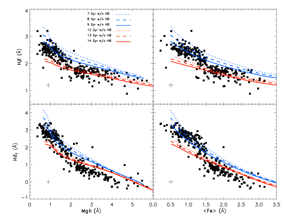
Figure 2: The distributions of 280 high S/N GCs (Caldwell et al. 2009, 2011) in the planes of Balmer indices (H$\beta$ and H$\delta_{F}$) against the metal indices (Mgb and $\langle$Fe$\rangle$) (a) the weaker metal-line group with stronger Balmer-lines and (b) the stronger metal-line group with weaker Balmer-lines. The division occurs at Mgb $\simeq$ 2.0, $\langle$Fe$\rangle$ $\simeq$ 1.5, H$\beta$$\simeq$1.8, and H$\delta_{F}$$\simeq$1.4, respectively. Overlaid YEPS models with varying ages that do not include the HB prescription are shown in blue for younger GCs (7, 8 , 9 Gyr) and in red for older GCs (12, 13, 14 Gyr). The models without HBs seems to invoke the age difference between the metal-poor and rich groups by as large as 6 Gyr.

Figure 1 presents our theoretical CMRs and IMRs. The stellar population simulations are based on the Yonsei Evolutionary Populations Synthesis (YEPS) model (Papers I, II, III, and IV; Chung et al., 2013). Predictions of absorption-line indices are constructed based on the widely used polynomial fitting functions parameterized in terms of $T_{\rm eff}$, log $g$, and [Fe/H]. YEPS models used in this study are computed with the fitting functions by Johansson et al. (2010, hereafter J10), that are based on the MILES stellar library (Sánchez-Blázquez et al., 2006). We adopt 12 Gyr old model clusters with the [$\alpha$/Fe] = 0.14 (Puzia et al., 2005; Chung et al., 2013). The solid lines represent model predictions that account for systematic HB star contribution. The dashed lines, on the other hand, represent models without a prescription for HB stars, for which post-RGB stars are absent. A test shows that adding a fixed HB type regardless of GC metallicity affect only the zero-point of colors and index strengths as expected. Such variations do not affect our conclusion drawn from Figure 1, as well as Figures 2 and 3. The YEPS model predictions using J10 fitting functions are given in Tables 1–5 for the indices Mgb, $\langle$Fe$\rangle$, H$\beta$, H$\gamma_{F}$, and H$\delta_{F}$ with and without the HB prescription.

The models in Figure 1 suggest that, because integrated light of main-sequence and RGB stars behave nonlinearly as a function of metallicity at given ages, the models without HB stars (dashed lines) exhibit some measure of nonlinearity. The wavy feature in the CMRs and IMRs is greatly enhanced when the HB effect is included (solid lines), increasing the sensitivity to metallicity at [Fe/H] $\simeq$ $-1$. For comparison, we overplot the observed $g-z$ and $u-z$ colors (Peacock et al., 2010) and the observed H$\delta_{F}$ and Mgb indices as functions of [Fe/H] (Caldwell et al., 2009, 2011). The values of [Fe/H] are derived from a bi-linear relation between $\langle$Fe$\rangle$ and [Fe/H] for the Milky Way GCs (Caldwell et al. 2011, see their Figure 8). The $g-z$ and $u-z$ colors respectively have 267 and 256 matched GCs with known spectroscopic [Fe/H]. Unfortunately, colors of M31 GCs are much more prone to uncertainties caused by extinction than spectral indices, showing too much scatter in the data to discern any meaningful relationship in comparison with the models. In contrast, the relations for H$\delta_{F}$ and Mgb are better defined by the data and they are reproduced reasonably well by the models.

It is clear in Figure 1 that the shape and slope of CMRs and IMRs depend on the choice of colors and indices due to their varying sensitivities to abundance and temperature. For the $g-z$ color (upper left panel), the models with HBs are bluer by 0.1 mag at most. Balmer index H$\delta_{F}$ (upper right), being one of the most temperature sensitive indices, is a prominent tracer of HB stars in a stellar population, thus displaying a much stronger wavy feature in the relation. The increase in line strength reaches up to 1.5 Å compared to the model prediction for H$\delta_{F}$ without HB star inclusion. The relative amount of shift brought on by HB stars in $g-z$ and H$\delta_{F}$ corresponds to almost 4 times higher sensitivity to HBs for H$\delta_{F}$ considering the length of the baselines. Interestingly enough, HB stars clearly also affect well-known metallicity indicators, $u-z$ and Mgb (bottom panels). The characteristics of $u$-band colors as metallicity tracer were explored in depth by Yi et al. (2004) and Paper II. The $u-z$ CMR displays less inflection in comparison with that of $g-z$, because $u$-band colors are relatively insensitive to temperature variation due to the Balmer Jump where $u$ band is located. Because the metal-line indices trace more directly the elemental abundance than colors do, the model predicts a relatively weaker wavy feature along the [Fe/H]–Mgb relation. The relative HB sensitivity of Mgb is about a half of that of $u-z$ considering the length of the baselines. However, this result demonstrates that the effect of HB stars on Mgb is certainly non-negligible. Therefore greater caution is required in deriving cluster metallicity directly from Mgb (see also Section 6 for more details).

4 THE NONLINEAR INDEX–INDEX RELATIONS AND HORIZONTAL BRANCHES

Figure 2 shows the distributions of 280 old, spheroidal component of M31 GCs (Caldwell et al., 2009, 2011) in the planes of Balmer indices (H$\beta$ and H$\delta_{F}$) against the metal indices (Mgb and $\langle$Fe$\rangle$). The observed data define highly nonlinear index–index relations and exhibit a division into two groups: (1) the weaker metal-line group with stronger Balmer-lines and (2) the stronger metal-line group with weaker Balmer-lines. The division occurs at Mgb $\simeq$ 2.0, $\langle$Fe$\rangle$ $\simeq$ 1.5, H$\beta$ $\simeq$ 1.8, and H$\delta_{F}$ $\simeq$ 1.4, respectively. We overlaid our models that do not include the HB prescription (Tables 1–5). The metal-rich group of GCs has weaker Balmer lines and is better explained by old (12, 13, and 14 Gyr) model lines than younger lines, albeit a slight offset for H$\delta_{F}$. On the other hand, the metal-poor GCs with stronger Balmer lines are predicted to have younger (7, 8, and 9 Gyr) ages. As a result, the models without HBs invoke the age difference between the metal-poor and rich groups by $\gtrsim$ 6 Gyr, with the metal-rich group being older. This seems inconsistent with the general notion of the age–metallicity relation that clusters with higher metallicities formed from more processed gas and thus are on average younger.

Figure 3 gives the single-age models that incorporate the HB prescriptions (solid lines, Tables 1–5). The overlaid model predictions (red solid, dotted lines) in the upper four panels represent the models based on the J10 fitting functions . Compared to cool stars, hotter stars have stronger Balmer-lines (reaching peaks at $\sim$10,000 K) and weaker metal-lines. The models predict that only metal-poor group contains hot ($>$ 8,000 K) HB stars, which leads to stronger Balmer lines and weaker metal lines than the models without HB stars (dashed lines). As a consequence, the model with HB stars features the wavy relations, reproducing the observed index–index behaviors.

In order to check whether the nonlinear feature depends on a particular choice of fitting functions, similar sets of simple stellar population (SSP) models are generated adopting two different sets of fitting functions presented by S07 and W94 and shown in the lower four panels of Figure 3. The model adopts the S07 fitting functions for all indices, that employed a more recent, superior spectral library (Jones, 1999) than W94. While the overall agreement between the two different sets of fitting functions are found to be good for most indices (S07; Chung et al., 2013), S07 fitting functions for Balmer lines yield a better match to observations at low metallicity than those of W94. For the limited cases of Mgb and $\langle$Fe$\rangle$, however, W94 is used, whose Mgb and $\langle$Fe$\rangle$ fitting functions render more sensitivity to the variation of [Fe/H] in the high temperature range of HB stars (6000 – 12000 K) and thus produce more inflected IMRs for these indices. The stellar population model based on the fitting functions by S07 and W94 also shows the wavy feature and reproduce the observed index–index relations very well.

Our theoretical rendition of M31 GC spectroscopy is supported by recent photometric studies. As our theoretical evidence asserts that HB stars are the main driver behind nonlinearity in index–index relations, the direct identification of HB stars on the CMDs of metal-poor GCs is confirmation of the model prediction. Individual stars in M31 GCs resolved by HST reveal HB morphology into the blue HB and the red HB through inspection of the CMDs (Rich et al., 2005; Perina et al., 2009, 2011). It is shown in Figure 3 that 11 metal-poor GCs with enhanced Balmer indices possess hot ($>$ 8,000 K) HB stars (blue squares), whereas six higher-metallicity GCs with weak Balmer lines do not (red squares). Further support for the presence of hot HB stars in metal-poor group of GCs in M31 comes from the integrated UV light by the GALEX space telescope (Kang et al., 2012). Hot HB stars are dominant UV sources in old GCs (O’Connell, 1999), and 27 metal-poor GCs with strong Balmer indices indeed show strong UV light ($NUV-V\,<\,3.5$ and $FUV-V\,<\,4.5$), corroborating the presence of hot HB stars in the metal-poor GCs (cyan squares). Three UV-weak ($NUV-V\,>\,4.5$ and $FUV-V\,>\,5.0$) GCs are identified (orange squares), one of which is a confirmed red-HB GC from its CMD (red squares). They all are located in the metal-rich region.

5 THE METALLICITY–INDEX NONLINEARITY AS ORIGIN OF INDEX BIMODALITY

As shown in Figures 2 and 3, the sample of 280 old, spheroidal component GCs of M31 exhibit a division into two groups. This Section examines how the nonlinear IMRs bring about the spectroscopic dichotomy of M31 GCs. Any viable scenario for the origin of the GC dichotomy should explain (1) the bimodality both in the metal-index and the Balmer-index distributions, and (2) the cause of the sharp difference in bimodality strength between metal- and Balmer-lines.

Figures 4$a$ and 4$b$ illustrate the process of conversion from the intrinsic metallicities to the indices via our theoretical metallicity–index relations. As in Figure 3, Figures 4$a$ and 4$b$ represent the models generated with the different fitting functions. Red model lines in Figure 4$a$ are based on J10 fitting functions and the orange model lines in Figure 4$b$ are of S07 and W94 fitting functions. For the underlying [Fe/H] spread, we make a simple assumption of a single Gaussian distribution of $10^{6}$ model GCs (top rows of Figures 4$a$ and 4$b$) to avoid small number statistics. The assumed mean and standard deviation of the Gaussian [Fe/H] function are respectively $-0.9$ and 0.6, and $-1.0$ and 0.5, which best reproduce the observed index distributions in the bottom rows of Figures 4$a$ and 4$b$. Observational uncertainties are taken into account in the simulation of the index distributions. The inflection in our theoretical [Fe/H]–index relations is visible not only for Balmer indices but also for Mgb. Such nonlinear feature has the effect of projecting the equi-distant metallicity intervals onto broader index intervals, causing scarcity in the index domain near the quasi-inflection point on each [Fe/H]–index relation.

As an aid to visualizing the simulated index distributions, we plot the indices of model GCs against their mass as an independent parameter (second rows of Figures 4$a$ and 4$b$). The divide between two vertical bands of GCs is visible and agrees well with the observed data. The resulting index histograms show bimodality both for Mgb and for Balmer indices with the scarcity at each quasi-inflection point reflected as dips (third rows of Figures 4$a$ and 4$b$). Given that the number of observed GCs is much smaller than that of the modeled ones, we repeat random sampling of 280 GCs from the $10^{6}$ model GC sample in order to assess the reliability of frequency of GCs in each bin. The gray shaded region in the index histograms (third rows of Figures 4$a$ and 4$b$) represent the estimated confidence intervals—one standard deviation of the 10,000 repeated samplings. Therefore we find good agreement between the theoretical predictions and the observations (bottom rows of Figures 4$a$ and 4$b$).

We perform mixture modeling analysis for a quantitative comparison between the distributions of 280 observed GCs and 10,000 randomly selected model GCs using GMM code (Gaussian Mixture Modeling, Muratove & Gnedin 2010). In addition to the general method of calculating the likelihood of a given data belonging to a mixture of two Gaussians (expressed in terms of $P(\chi^{2})$, Ashman et al. 1994). GMM provides further statistical tests of bimodality in forms of $DD$, a measure of separation between peaks relative to their widths, and kurtosis, a measure of peakedness of a given distribution. The kurtosis statistic assesses whether a distribution is bimodal such that a negative kurtosis corresponds to a more flattened shape of the sum of two populations. Note that kurt$\,<\,0$ is a necessary but not sufficient condition of bimodality. Table 6 presents the resulting GMM outputs. Bimodality is preferred for Mgb distributions for observed and simulated GCs ($P(\chi^{2})=0.001-0.01$). The fraction of GCs assigned to the metal-rich group is similar for the observation and simulations (i.e., $59\,\%\sim 64\,\%$). The observed and the simulated distributions of H$\beta$, H$\gamma_{F}$, and H$\delta_{F}$ are shown to be bimodal at the $99.9\,\%$ level, displaying two distinct peaks. For all three Balmer lines, the metal-poor peaks are slightly more dominant with the simulations consistently predicting lower fractions of metal-rich GCs compared to the observation. On the whole, we find good agreement between the observation and the models.

We note that the offset between the models and the observation are translated to the shift in peak locations in the simulated index distributions. Our stellar population models show that, for given input parameters, the absolute quantities of output are rather subject to the choice of model ingredients such as stellar evolutionary tracks, flux libraries, and fitting functions, and the different choices can result in up to $\sim$ 0.4 Å variation in Mgb and Balmer strengths. Hence, we put more weight on the relative index values, i.e., the number ratios between index-weak and strong GCs and the overall morphologies of the simulated index histograms. The recent work by Chung et al. (2013) discusses the systematic effects exerted by varying MDFs and ages, as well as the use of different stellar population models on the projected index distributions (see their Figures 20–23). The cases for different choices of model ingredients are also addressed in Section 3 of the same paper (see their Figure 5).

In Figure 5, we apply the identical projection scheme to the actual data of the [Fe/H] distribution comprised of 280 old GCs in M31. Using the observed [Fe/H] distribution, we examine the index distributions produced by conventional linear fit and by projection through the model relations. The observed [Fe/H] distribution (the grey histograms along the $y$-axes of all panels) is best described by a single Gaussian with the mean and standard deviation of $-1.05$ and 0.57, which agree well with those of the modeled [Fe/H]’s in Figure 4. It is noteworthy that the observed, unimodal [Fe/H] histogram is at odds with the popular view, in which GC systems consist of two groups with different metallicities. With such an underlying metallicity spread, the indices converted via the conventional linear fit to the observed [Fe/H] versus index data are bound to have unimodal index distributions (second row), and thus inconsistent with the observations. In contrast, our theoretical [Fe/H]–index relations produce clear bimodality in the Balmer and Mgb index distributions for both models with J10 fitting functions (third row) and the models with S07 and W94 (bottom row).

Table 7 lists our GMM analysis of Figure 5. The observations and the non-linear transformations through two model sets are bimodal with GMM probabilities of $99.9\,\%$. For Mgb, sharper metal-poor peaks are reflected in somewhat less significant $P({\it kurt})$ values. Unlike in Figure 4, the simulations predict higher fractions of metal-rich GCs compared to the observations. In the case of linear transformations, GMM finds the probabilities of rejecting unimodal Gaussian to be insignificant ($P(\chi^{2})=0.46-0.47$). Most of the GCs ($>\,94\,\%$) are assigned to either the metal-poor group (Mgb) or the metal-rich group (Balmer lines).

6 THE INDEX–METALLICITY NONLINEARITY AND SPECTROSCOPIC METALLICITIES

Previous spectroscopic studies of extragalactic GC systems have made use of metal-line indices such as Mgb and a composite [MgFe]^′ index as proxies to cluster metallicity (e.g., Strader et al., 2007; Woodley et al., 2010). In case of NGC 5128 GC system, for instance, Woodley et al. (2010) found that bimodality is preferred for their measured [MgFe]^′. Because [MgFe]^′ index is obtained directly from high-quality spectra of NGC 5128 GCs and known to be almost independent of [$\alpha$/Fe], they concluded that their bimodal [MgFe]^′ distribution indicates the existence of two distinct metallicity subpopulations. However, we have shown that the strengths of absorption line indices are affected in varying degrees by hot HB stars in old stellar populations according to their respective responses to HB temperature. We have subsequently demonstrated both theoretically and observationally that the nonlinearity in the [Fe/H]–index relations can generate bimodal index distributions, even for the Mgb index, from unimodal metallicity spread.

More importantly, Balmer lines exhibit very strong bimodal index distributions, which are translated routinely into bimodal metallicity distributions. Most studies have derived spectroscopic [Fe/H]’s based jointly on metal-lines and Balmer lines: finding best-fitting age, metallicity, and [$\alpha$/Fe] through multivariate fits to SSP models and/or an iterative method using the grids of Balmer lines and metal-sensitive indices (e.g., Puzia et al., 2005; Cenarro et al., 2007; Beasley et al., 2008; Park et al., 2012). Therefore, Balmer lines have played an important role in establishing the notion of bimodality in spectroscopic metallicity. In light of this, the previous view of the absorption indices being linear metallicity tracers requires modification (Chung et al., 2013), and a revisit to spectroscopic metallicity measurements of GCs may prove worthwhile.

Figure 6 attempts at obtaining metallicity distributions by inversely transforming each individual index distributions to metallicities. The process of inverse conversion involves complication arising from the incompleteness of the current models, in that the visible offsets between observations and models result in the slight offsets in the peak positions. Considering the caveat, the model incompleteness allows room for displacement of the models within a few tenth of an Å ($<\,\left|0.4\right|$ Å), for more accurate simulations of MDFs. We displace the model lines in both directions along x-axis ($<\,\left|0.4\right|$ Å) in steps of 0.01 Å, then determine the best-fit $\chi^{2}_{min}$ to the observed data. Gaussian kernel smoothing is applied to the observation (top row) in order to reduce the stochastic variations. These kernelled data of observed index distributions are transformed via the models that are now displaced accordingly to the amount determined for each index. The red solid lines and the orange dahsed lines in the second row correspond to the models based on fitting functions of J10 and fitting functions of S07 and W94, respectively, and the resulting MDFs are shown as red and orange histograms in the fourth and bottom row. The MDFs derived from Mgb exhibit broad unimodal distributions. The MDFs inferred from Balmer lines show similar unimodal shapes with somewhat extended metal-rich wings, which appears consistent with the observed MDF in Figure 5. We note that, in contradiction to the visual impression, the values of $P(\chi^{2})$ indicate a high probability of bimodality for the inferred MDFs (Table 8). Muratov & Gnedin (2010) discusses the limitations of the $P(\chi^{2})$, and states that “GMM is more a test of Gaussianity than of unimodality”. The $P(DD)$ and $P({\it kurt})$, however, validate the preferred unimodal distributions over bimodal ones. On the contrary to the above cases, linear conversions (blue dotted lines in the second row) preserve the morphology of each index distribution, and exhibit strong bimodality in inferred metallicity distributions (blue histograms in the third row), which is inconsistent with the observation. This issue entails far-reaching implications and will be fully explored in a forthcoming paper (S. Kim et al. 2013, Paper VI in preparation).

7 DISCUSSION

We show that the spectroscopic dichotomy of the M31 GCs emerges not necessarily because of any division in physical parameters of GCs such as metallicity and age. Instead, the phenomenon is most likely attributed to the difference in the hot HB proportion of stellar populations, which is a strong nonlinear function of GC metallicity and increases abruptly in metal-poor GCs. The large hot star fraction of metal-poor GCs simultaneously makes metal-lines weaker and Balmer-lines stronger than they otherwise might be. As a result, GCs that have the index values around the midpoint of distributions are relatively scarce, which explains the bimodality in index distributions. The results that are based on spectroscopy—a more detailed probe into stellar contents in GCs—are consistent with the view that the nonlinear metallicity-to-color transformation is responsible for photometric color bimodality of GCs (Papers I, II, III, and IV).

Perhaps the strongest argument against our scenario for the spectroscopic division of M31 GCs comes from our Milky Way, which is a similar disk galaxy and serves as a prime example of confirmed two GC groups present (Harris et al., 2006). Despite many similarities shared by the two galaxies, however, there is increasing evidence that the spheroidal components of M31 and our Galaxy have distinct characteristics. For instance, extensive investigations into the kinematics of GCs and planetary nebulae suggest that M31 is a bulge-dominant disk galaxy, unlike the Milky Way (Hurley-Keller et al., 2004; Merrett et al., 2006; Lee et al., 2008b). These studies revealed a general trend of increasing velocity dispersion for M31 GCs with distance, indicating the presence of a system of pressure-supported, dynamically hot halo. Furthermore, spectroscopic analyses showed that metallicity distribution of old M31 GCs differs from that of the Galactic GCs in that the M31 GC system lacks bimodality in its metallicity distribution (Caldwell et al., 2011; Galleti et al., 2009). Therefore, M31’s spheroid does not seem to have the same GC formation history as that of the Milky Way and, the two galaxies do not necessarily share the common origin of the GC division.

Hierarchical models for galaxy formation depict the shaping of a single massive galaxy through merging of thousands of lower-mass building blocks. This picture may leave little room for the possibility of a GC system containing merely two subpopulations. Indeed, the continuous nature of the physical parameters of old GCs in M31 can stem from its virtually continuous chemical evolution early on ($\sim$ 12 Gyr ago). The chemical enrichment seems to have been achieved on a relatively short timescale via many successive rounds of early, vigorous star formation in M31 halo’s history. Interestingly, the old, spheroidal component of the M31 GC system used in this study is associated chiefly with the galaxy’s bulge, and hence can be viewed as an analogy to GC systems belonging to typical elliptical galaxies. Large elliptical galaxies were the sites where the GC color bimodality was first discovered, and ever since ellipticals have been believed to harbor two groups of GCs with different genesis. Our findings challenge such conventional wisdom, and the new insight into the structure of GC systems greatly simplifies theories of galaxy formation.

Figure 1: Empirical and theoretical color-metallicity relations and index-metallicity relations. Red curves are the 12 Gyr old Yonsei Evolutionary Populations Synthesis (YEPS) model (Paper II; Chung et al. 2012) depicting models including the prescriptions for HB stars. Blue lines represent the 12 Gyr old model clusters without inclusion of HB stars. The theoretical CMRs are a fifth-order polynomial fit to the model data. The $\alpha$-element enhancement parameter, [$\alpha$/Fe], is assumed to be 0.14 (Puzia et al. 2005). Photometry for $u$ (ABMAG), $g$ (ABMAG), and $z$ (ABMAG) mags for GC candidates in the left panels are from SDSS catalog (Peacock et al. 2010). Using the archival images, Peacock et al. (2010) performed photometry for the candidate clusters listed in Revised Bologna Catalog (RBC v4.0, Galleti et al. 2004). The averaged $E(B-V)$ from Barmby et al. (2000), Fan et al. (2008) and Caldwell et al. (2011) are adopted for dereddening. The arrow represents a reddening of $E(B-V)=0.1$. 267 and 256 matches against spectroscopically derived [Fe/H] (Caldwell et al., 2009, 2011) were found for $g-z$ and $u-z$ colors, respectively. For H$\delta_{F}$ and Mgb, 280 high S/N, old clusters of M31 (Caldwell et al., 2009, 2011) are used. For a better comparison with color, x-axis for H$\delta_{F}$ is in reverse order.

Figure 3: Same as Figure 2 but the correlations between Balmer-line indices (H$\beta$ and H$\delta_{F}$) and metal-line indices (Mgb and $\langle$Fe$\rangle$) for M31 GCs are compared with the single-age models with HB star inclusion (solid lines) and without HB star inclusion (dashed lines). In the lower panel, the YEPS models use the functions presented by S07 for Balmer indices, while the models adopt W94 for metal line indices Mgb and $\langle$Fe$\rangle$ (orange solid and dotted lines). Top left of each 2-by-2 panel: the H$\beta$–Mgb relation for 280 GCs (gray squares). The error bars show the mean observational uncertainties. 11 blue squares are GCs containing hot ($>$ 8,000 K) HB stars confirmed by their color-magnitude diagrams with Hubble Space Telescope, and six red squares are GCs without hot HB stars (Rich et al., 2005; Perina et al., 2009, 2011). Cyan and orange squares represent 27 UV-strong ($NUV-V\,<\,3.5$ and $FUV-V\,<\,4.5$) and three UV-weak ($NUV-V\,>\,4.5$ and $FUV-V\,>\,5.0$) GCs identified in the GALEX UV photometric studies, respectively (Kang et al. 2012; Rey et al. 2007; RBC v4.0, Galleti et al. 2004). Five GCs are in common in the HST and GALEX observations. The overlaid lines represent our model predictions for 12 Gyr old GCs with the [$\alpha$/Fe] = 0.14 (Puzia et al. 2005). Bottom left of each panel: same as (Top left), but for the H$\delta_{F}$–Mgb relation. Top right of each panel: same as (Top left), but for the H$\beta$–$\langle$Fe$\rangle$ relation. Bottom right of each panel: same as (Top left), but for the H$\delta_{F}$–$\langle$Fe$\rangle$ relation.

Figure 4: $a$. Monte-Carlo simulations of the indices (Mgb, H$\beta$, H$\gamma_{F}$, and H$\delta_{F}$) distributions for $10^{6}$ model GCs. Top row: the correlation between [Fe/H] and Mgb, H$\beta$ and H$\delta_{F}$ for the identical M31 GC sample in Figure 2, overlaid with the model with the HB prescription (red solid lines). A single Gaussian distribution along the y-axis represents the underlying metallicity distribution. Second row: indices vs. stellar mass diagram for 5000 randomly selected model GCs (gray dots) and the observed M31 GCs (black dots) (RBC v4). Indices are derived based on the metallicity distribution and theoretical index–[Fe/H] relations shown in top row. Stellar masses of GCs are derived from the integrated V-band absolute magnitudes (Caldwell et al. 2011), assuming a Gaussian luminosity function ($\langle$$M_{V}$$\rangle$ = $-6.72$ and $\sigma({M_{V}})$ = 1.5) for $M_{V}$. Third row: the resultant index distribution for $10^{6}$ model GCs. The bin sizes for each index distribution range from 0.01 to 0.03 Å. Observational uncertainties are taken into account in the simulation of the index distributions. Given that the number of observed GCs is much smaller, 280 GCs from the $10^{6}$ model GCs are drawn randomly to estimate the possible ranges of simulated index distributions. The sampling is carried out 10,000 times for each index, and the grey shaded bands show the $1\sigma$ range of individual bins. The mean observational error is adopted for the bin size. Bottom row: the observed index distributions for 280 GCs. The mean error is adopted for the bin width, and a Gaussian density kernel estimate is shown by solid line. $b$. Same as Figure 4$a$ but using the models computed with S07 and W94 fitting functions (orange solid lines).

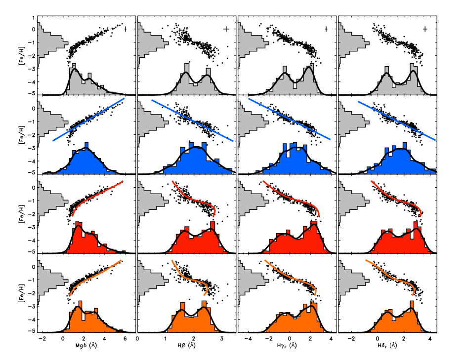
Figure 5: Comparison of simulated indices (Mgb, H$\beta$, H$\gamma_{F}$, and H$\delta_{F}$) distributions with the M31 GC observations. Top row: the index–[Fe/H] relations for the identical sample in Figure 2. The observed distributions of [Fe/H] and indices are shown along the y-axis and x-axis, respectively. Second row: the observed [Fe/H] histograms along the y-axes are the same as in the top row but the transformed index distribution (blue histogram) using a simple linear fit (blue solid lines) to the data. Third row: the transformed index distribution (red histogram) using our theoretical [Fe/H]–index relation (red solid lines). Bottom row: the transformed index distribution (orange histogram) using our theoretical [Fe/H]–index relation (orange solid lines) based on S07 and W94 fitting functions.

Figure 6: Mgb, H$\beta$, H$\gamma_{F}$, and H$\delta_{F}$ distributions and their inferred metallicity distributions for the M31 GC system. Top row: Gaussian kernel smoothing is applied to the observed index distributions. Second row: color scheme is the same as in Figure 5. Solid red lines represent theoretical [Fe/H]–index relations computed with J10 fitting functions displaced by –0.29 Å, –0.05 Å, –0.33 Å, and –0.18 Å for Mgb, H$\beta$, H$\gamma_{F}$, and H$\delta_{F}$, respectively. Dashed orange lines represent theoretical [Fe/H]–index relations with S07 and W94 fitting functions offset by –0.31 Å, 0.12 Å, –0.19 Å, and 0.04 Å for Mgb, H$\beta$, H$\gamma_{F}$, and H$\delta_{F}$, respectively. The blue dotted lines represent the linear fits to the kernelled data in the top row. Third row: metallicity distributions obtained from each index, Mgb, H$\beta$, H$\gamma_{F}$, and H$\delta_{F}$ via linear transformations are shown as blue histograms. Fourth row: metallicity distributions obtained from each index using the models with J10 fitting functions are shown as red histograms. Bottom row: metallicity distributions obtained from each index using the models based on S07 and W94 fitting functions are shown as orange histograms.

Table 1: The M$g{\it b}$ of the YEPS model GCs without ($w/o$) and with ($w$) HBs for [$\alpha$/Fe] = 0.14 and ages ($t$) of 7, 8, 9, 12, 13, and 14 Gyr. The models are computed using J10 fitting functions.

[Fe/H]	Mgb
	$t$ = 7		8		9		12		13		14
	$w/o$	$w$	$w/o$	$w$	$w/o$	$w$	$w/o$	$w$	$w/o$	$w$	$w/o$	$w$
–2.5	0.637	0.622	0.642	0.628	0.649	0.631	0.688	0.664	0.710	0.690	0.738	0.721
–2.4	0.692	0.673	0.702	0.682	0.713	0.689	0.765	0.736	0.791	0.767	0.822	0.803
–2.3	0.750	0.729	0.764	0.740	0.779	0.748	0.842	0.807	0.872	0.844	0.907	0.883
–2.2	0.802	0.778	0.819	0.791	0.837	0.799	0.912	0.870	0.945	0.912	0.984	0.957
–2.1	0.844	0.819	0.864	0.833	0.886	0.844	0.973	0.923	1.011	0.972	1.052	1.022
–2.0	0.879	0.853	0.904	0.871	0.930	0.884	1.030	0.971	1.071	1.026	1.116	1.080
–1.9	0.912	0.885	0.942	0.909	0.974	0.928	1.088	1.020	1.133	1.081	1.181	1.140
–1.8	0.950	0.921	0.987	0.951	1.025	0.976	1.154	1.073	1.202	1.143	1.252	1.207
–1.7	1.000	0.969	1.044	1.006	1.090	1.038	1.235	1.140	1.285	1.217	1.337	1.287
–1.6	1.066	1.032	1.119	1.076	1.173	1.116	1.334	1.223	1.387	1.307	1.439	1.385
–1.5	1.153	1.115	1.215	1.168	1.278	1.214	1.455	1.326	1.511	1.420	1.565	1.506
–1.4	1.262	1.222	1.335	1.283	1.406	1.336	1.601	1.448	1.660	1.544	1.715	1.640
–1.3	1.394	1.353	1.478	1.423	1.558	1.484	1.771	1.592	1.833	1.689	1.890	1.798
–1.2	1.548	1.503	1.642	1.580	1.731	1.650	1.964	1.754	2.029	1.839	2.089	1.960
–1.1	1.720	1.663	1.824	1.747	1.923	1.824	2.177	1.930	2.246	1.995	2.309	2.129
–1.0	1.906	1.833	2.021	1.922	2.128	2.007	2.405	2.121	2.480	2.168	2.547	2.295
–0.9	2.103	2.030	2.227	2.127	2.344	2.218	2.644	2.367	2.726	2.395	2.799	2.483
–0.8	2.306	2.238	2.440	2.342	2.566	2.439	2.890	2.617	2.980	2.639	3.060	2.681
–0.7	2.513	2.450	2.655	2.561	2.790	2.666	3.140	2.880	3.237	2.902	3.326	2.915
–0.6	2.721	2.667	2.871	2.787	3.014	2.899	3.390	3.150	3.495	3.180	3.592	3.177
–0.5	2.929	2.883	3.088	3.015	3.238	3.136	3.637	3.418	3.751	3.469	3.856	3.469
–0.4	3.139	3.103	3.305	3.243	3.462	3.371	3.882	3.679	4.003	3.732	4.116	3.770
–0.3	3.353	3.326	3.525	3.473	3.688	3.608	4.124	3.931	4.251	4.003	4.370	4.050
–0.2	3.572	3.553	3.751	3.705	3.918	3.845	4.364	4.185	4.496	4.271	4.619	4.331
–0.1	3.802	3.784	3.986	3.942	4.156	4.081	4.605	4.438	4.737	4.528	4.862	4.602
0.0	4.044	4.024	4.232	4.184	4.403	4.322	4.846	4.689	4.976	4.783	5.099	4.865
0.1	4.298	4.270	4.489	4.433	4.660	4.574	5.088	4.940	5.212	5.034	5.329	5.115
0.2	4.559	4.523	4.752	4.690	4.919	4.829	5.326	5.185	5.441	5.274	5.550	5.346
0.3	4.815	4.779	5.008	4.948	5.170	5.086	5.550	5.415	5.655	5.495	5.754	5.564
0.4	5.046	5.010	5.234	5.178	5.390	5.312	5.743	5.613	5.838	5.683	5.927	5.749
0.5	5.214	5.188	5.394	5.347	5.543	5.474	5.878	5.753	5.967	5.819	6.051	5.875

.

Table 2: $\langle$Fe$\rangle$ of the YEPS model GCs without ($w/o$) and with ($w$) HBs for [$\alpha$/Fe] = 0.14 and ages ($t$) of 7, 8, 9, 12, 13, and 14 Gyr. The models are computed using J10 fitting functions.

[Fe/H]	$\langle$Fe$\rangle$
	$t$ = 7		8		9		12		13		14
	$w/o$	$w$	$w/o$	$w$	$w/o$	$w$	$w/o$	$w$	$w/o$	$w$	$w/o$	$w$
–2.5	0.498	0.462	0.495	0.460	0.493	0.459	0.495	0.477	0.500	0.487	0.509	0.498
–2.4	0.516	0.481	0.517	0.480	0.518	0.477	0.527	0.507	0.535	0.519	0.545	0.533
–2.3	0.538	0.504	0.542	0.505	0.546	0.501	0.562	0.538	0.571	0.553	0.581	0.568
–2.2	0.564	0.531	0.572	0.535	0.579	0.531	0.603	0.574	0.613	0.591	0.624	0.608
–2.1	0.597	0.566	0.609	0.572	0.620	0.571	0.652	0.615	0.663	0.638	0.676	0.657
–2.0	0.637	0.610	0.653	0.619	0.667	0.620	0.709	0.664	0.723	0.693	0.738	0.716
–1.9	0.686	0.661	0.705	0.675	0.723	0.681	0.775	0.721	0.793	0.757	0.811	0.786
–1.8	0.742	0.719	0.765	0.737	0.787	0.748	0.851	0.784	0.872	0.829	0.894	0.864
–1.7	0.806	0.785	0.834	0.808	0.860	0.824	0.934	0.855	0.959	0.909	0.984	0.950
–1.6	0.877	0.858	0.909	0.884	0.940	0.904	1.025	0.931	1.053	0.993	1.080	1.043
–1.5	0.955	0.937	0.992	0.967	1.027	0.991	1.122	1.015	1.152	1.082	1.181	1.140
–1.4	1.038	1.022	1.080	1.056	1.120	1.084	1.224	1.103	1.255	1.167	1.285	1.233
–1.3	1.127	1.112	1.174	1.151	1.218	1.183	1.330	1.196	1.362	1.252	1.391	1.327
–1.2	1.219	1.208	1.271	1.249	1.319	1.286	1.438	1.301	1.470	1.333	1.498	1.411
–1.1	1.316	1.307	1.372	1.352	1.423	1.393	1.548	1.416	1.580	1.422	1.607	1.493
–1.0	1.415	1.410	1.475	1.457	1.530	1.502	1.660	1.539	1.691	1.529	1.716	1.575
–0.9	1.518	1.517	1.580	1.567	1.637	1.614	1.772	1.670	1.804	1.651	1.829	1.660
–0.8	1.623	1.630	1.687	1.681	1.747	1.729	1.886	1.799	1.919	1.782	1.944	1.761
–0.7	1.732	1.747	1.797	1.798	1.858	1.847	2.002	1.934	2.036	1.921	2.064	1.887
–0.6	1.845	1.871	1.910	1.922	1.971	1.971	2.120	2.070	2.158	2.071	2.189	2.035
–0.5	1.962	2.000	2.026	2.053	2.088	2.101	2.243	2.210	2.284	2.225	2.320	2.209
–0.4	2.085	2.139	2.148	2.189	2.209	2.238	2.371	2.355	2.417	2.379	2.460	2.387
–0.3	2.214	2.284	2.277	2.335	2.337	2.383	2.505	2.510	2.557	2.538	2.607	2.558
–0.2	2.351	2.439	2.413	2.489	2.473	2.537	2.647	2.670	2.705	2.706	2.763	2.738
–0.1	2.496	2.601	2.558	2.649	2.618	2.702	2.799	2.839	2.862	2.885	2.926	2.926
0.0	2.649	2.768	2.713	2.818	2.773	2.874	2.960	3.016	3.027	3.067	3.097	3.117
0.1	2.811	2.944	2.877	2.994	2.939	3.050	3.130	3.198	3.200	3.253	3.272	3.308
0.2	2.981	3.121	3.049	3.174	3.114	3.233	3.308	3.383	3.377	3.439	3.450	3.497
0.3	3.155	3.305	3.228	3.361	3.295	3.417	3.491	3.572	3.558	3.627	3.627	3.683
0.4	3.330	3.483	3.407	3.547	3.478	3.599	3.672	3.759	3.736	3.813	3.799	3.864
0.5	3.500	3.655	3.581	3.718	3.653	3.777	3.846	3.939	3.905	3.988	3.962	4.038

.

Table 3: The H$\beta$ of the YEPS model GCs without ($w/o$) and with ($w$) HBs for [$\alpha$/Fe] = 0.14 and ages ($t$) of 7, 8, 9, 12, 13, and 14 Gyr. The models are computed using J10 fitting functions.

[Fe/H]	H$\beta$
	$t$ = 7		8		9		12		13		14
	$w/o$	$w$	$w/o$	$w$	$w/o$	$w$	$w/o$	$w$	$w/o$	$w$	$w/o$	$w$
–2.5	3.336	3.368	3.052	3.207	2.810	3.211	2.287	2.613	2.169	2.365	2.075	2.202
–2.4	3.299	3.292	3.019	3.126	2.780	3.128	2.270	2.624	2.154	2.374	2.062	2.196
–2.3	3.264	3.221	2.987	3.049	2.753	3.039	2.253	2.647	2.140	2.375	2.048	2.195
–2.2	3.226	3.167	2.954	2.986	2.725	2.950	2.236	2.673	2.124	2.388	2.033	2.195
–2.1	3.182	3.109	2.916	2.923	2.692	2.854	2.215	2.698	2.105	2.395	2.015	2.189
–2.0	3.132	3.045	2.871	2.854	2.654	2.754	2.191	2.722	2.083	2.408	1.993	2.184
–1.9	3.074	2.975	2.820	2.780	2.610	2.656	2.162	2.737	2.057	2.409	1.968	2.169
–1.8	3.010	2.906	2.763	2.712	2.560	2.579	2.130	2.746	2.028	2.410	1.940	2.154
–1.7	2.941	2.831	2.701	2.640	2.506	2.500	2.094	2.738	1.996	2.407	1.910	2.136
–1.6	2.867	2.760	2.636	2.575	2.448	2.437	2.055	2.725	1.961	2.409	1.878	2.109
–1.5	2.792	2.688	2.569	2.508	2.389	2.374	2.014	2.689	1.924	2.400	1.844	2.076
–1.4	2.715	2.612	2.501	2.440	2.328	2.309	1.971	2.629	1.886	2.446	1.810	2.091
–1.3	2.639	2.538	2.434	2.374	2.269	2.246	1.927	2.545	1.846	2.484	1.775	2.106
–1.2	2.566	2.466	2.369	2.308	2.210	2.183	1.883	2.406	1.806	2.527	1.739	2.187
–1.1	2.495	2.398	2.307	2.245	2.154	2.124	1.838	2.243	1.765	2.491	1.703	2.266
–1.0	2.427	2.334	2.248	2.186	2.101	2.067	1.795	2.080	1.725	2.357	1.666	2.328
–0.9	2.363	2.271	2.192	2.129	2.051	2.014	1.752	1.931	1.684	2.175	1.628	2.351
–0.8	2.302	2.209	2.140	2.075	2.003	1.962	1.710	1.824	1.643	1.990	1.590	2.285
–0.7	2.244	2.150	2.089	2.022	1.957	1.914	1.669	1.732	1.603	1.830	1.550	2.136
–0.6	2.187	2.093	2.041	1.973	1.913	1.865	1.629	1.662	1.563	1.683	1.510	1.908
–0.5	2.132	2.039	1.992	1.924	1.870	1.820	1.590	1.606	1.523	1.584	1.469	1.679
–0.4	2.076	1.984	1.944	1.875	1.826	1.776	1.551	1.559	1.484	1.523	1.427	1.530
–0.3	2.018	1.933	1.894	1.827	1.782	1.734	1.514	1.518	1.445	1.472	1.386	1.448
–0.2	1.959	1.878	1.841	1.780	1.736	1.691	1.477	1.480	1.407	1.428	1.346	1.390
–0.1	1.897	1.820	1.787	1.729	1.688	1.645	1.441	1.443	1.371	1.388	1.308	1.343
0.0	1.834	1.761	1.731	1.677	1.639	1.598	1.406	1.405	1.337	1.351	1.272	1.302
0.1	1.771	1.697	1.674	1.619	1.590	1.544	1.373	1.363	1.305	1.310	1.239	1.260
0.2	1.711	1.633	1.620	1.559	1.543	1.489	1.341	1.323	1.276	1.272	1.210	1.221
0.3	1.658	1.573	1.573	1.503	1.501	1.441	1.313	1.288	1.250	1.237	1.184	1.186
0.4	1.619	1.529	1.538	1.460	1.470	1.407	1.290	1.258	1.228	1.208	1.162	1.155
0.5	1.602	1.507	1.522	1.442	1.455	1.386	1.273	1.234	1.209	1.182	1.143	1.127

.

Table 4: The H$\gamma_{F}$ of the YEPS model GCs without ($w/o$) and with ($w$) HBs for [$\alpha$/Fe] = 0.14 and ages ($t$) of 7, 8, 9, 12, 13, and 14 Gyr. The models are computed using J10 fitting functions.

[Fe/H]	H$\gamma_{F}$
	$t$ = 7		8		9		12		13		14
	$w/o$	$w$	$w/o$	$w$	$w/o$	$w$	$w/o$	$w$	$w/o$	$w$	$w/o$	$w$
–2.5	4.035	4.137	3.586	3.897	3.193	3.901	2.307	2.883	2.092	2.454	1.912	2.154
–2.4	3.924	3.957	3.475	3.709	3.083	3.721	2.202	2.841	1.988	2.405	1.809	2.073
–2.3	3.821	3.784	3.369	3.521	2.976	3.523	2.097	2.822	1.886	2.341	1.709	2.005
–2.2	3.712	3.639	3.259	3.355	2.865	3.320	1.988	2.810	1.780	2.304	1.606	1.940
–2.1	3.589	3.485	3.136	3.179	2.744	3.089	1.872	2.798	1.666	2.251	1.493	1.862
–2.0	3.449	3.314	2.998	2.989	2.609	2.837	1.747	2.781	1.542	2.213	1.370	1.784
–1.9	3.291	3.122	2.844	2.785	2.461	2.580	1.613	2.751	1.410	2.151	1.237	1.684
–1.8	3.116	2.930	2.676	2.587	2.300	2.358	1.470	2.711	1.268	2.091	1.095	1.584
–1.7	2.928	2.723	2.495	2.378	2.128	2.123	1.318	2.638	1.119	2.024	0.946	1.477
–1.6	2.730	2.521	2.304	2.179	1.947	1.924	1.158	2.558	0.963	1.971	0.792	1.353
–1.5	2.524	2.314	2.107	1.975	1.758	1.718	0.993	2.436	0.803	1.895	0.636	1.219
–1.4	2.314	2.098	1.905	1.764	1.564	1.507	0.822	2.266	0.638	1.938	0.477	1.199
–1.3	2.101	1.881	1.701	1.553	1.368	1.294	0.647	2.045	0.471	1.964	0.317	1.177
–1.2	1.888	1.662	1.495	1.336	1.169	1.079	0.469	1.705	0.301	1.999	0.156	1.314
–1.1	1.673	1.444	1.289	1.121	0.970	0.864	0.290	1.283	0.130	1.869	–0.006	1.442
–1.0	1.457	1.229	1.083	0.906	0.771	0.652	0.108	0.826	–0.044	1.519	–0.170	1.529
–0.9	1.240	1.007	0.876	0.691	0.571	0.437	–0.074	0.366	–0.219	1.035	–0.336	1.526
–0.8	1.019	0.778	0.668	0.471	0.372	0.221	–0.257	–0.006	–0.396	0.508	–0.507	1.312
–0.7	0.794	0.545	0.458	0.250	0.171	0.007	–0.441	–0.350	–0.576	–0.004	–0.682	0.877
–0.6	0.564	0.307	0.244	0.030	–0.031	–0.211	–0.624	–0.627	–0.757	–0.505	–0.861	0.187
–0.5	0.327	0.067	0.025	–0.195	–0.235	–0.424	–0.808	–0.866	–0.940	–0.879	–1.045	–0.539
–0.4	0.083	–0.179	–0.198	–0.420	–0.441	–0.635	–0.992	–1.081	–1.124	–1.149	–1.232	–1.072
–0.3	–0.166	–0.416	–0.425	–0.643	–0.651	–0.839	–1.175	–1.288	–1.308	–1.375	–1.422	–1.404
–0.2	–0.420	–0.658	–0.656	–0.862	–0.862	–1.045	–1.358	–1.477	–1.491	–1.581	–1.611	–1.659
–0.1	–0.675	–0.900	–0.889	–1.081	–1.076	–1.254	–1.539	–1.656	–1.672	–1.771	–1.797	–1.872
0.0	–0.928	–1.135	–1.122	–1.301	–1.289	–1.460	–1.717	–1.827	–1.849	–1.944	–1.978	–2.055
0.1	–1.174	–1.366	–1.350	–1.515	–1.500	–1.655	–1.893	–1.990	–2.020	–2.104	–2.150	–2.221
0.2	–1.407	–1.579	–1.569	–1.716	–1.705	–1.844	–2.065	–2.148	–2.185	–2.257	–2.311	–2.373
0.3	–1.622	–1.779	–1.775	–1.907	–1.901	–2.019	–2.231	–2.303	–2.343	–2.404	–2.461	–2.512
0.4	–1.812	–1.949	–1.961	–2.079	–2.082	–2.181	–2.391	–2.452	–2.493	–2.545	–2.600	–2.642
0.5	–1.974	–2.096	–2.121	–2.224	–2.242	–2.330	–2.543	–2.597	–2.638	–2.683	–2.732	–2.768

.

Table 5: The H$\delta_{F}$ of the YEPS model GCs without ($w/o$) and with ($w$) HBs for [$\alpha$/Fe] = 0.14 and ages ($t$) of 7, 8, 9, 12, 13, and 14 Gyr. The models are computed using J10 fitting functions.

[Fe/H]	H$\delta_{F}$
	$t$ = 7		8		9		12		13		14
	$w/o$	$w$	$w/o$	$w$	$w/o$	$w$	$w/o$	$w$	$w/o$	$w$	$w/o$	$w$
–2.5	4.163	4.142	3.715	3.875	3.337	3.864	2.529	3.157	2.342	2.746	2.186	2.459
–2.4	4.082	4.021	3.643	3.751	3.275	3.736	2.492	3.175	2.310	2.766	2.157	2.447
–2.3	4.001	3.898	3.570	3.622	3.211	3.594	2.451	3.210	2.275	2.761	2.127	2.444
–2.2	3.910	3.791	3.488	3.505	3.137	3.444	2.399	3.241	2.230	2.779	2.088	2.440
–2.1	3.805	3.669	3.392	3.377	3.051	3.273	2.336	3.266	2.172	2.776	2.035	2.417
–2.0	3.684	3.531	3.283	3.233	2.952	3.086	2.261	3.278	2.102	2.781	1.968	2.388
–1.9	3.548	3.378	3.160	3.076	2.841	2.893	2.175	3.272	2.020	2.760	1.889	2.336
–1.8	3.400	3.222	3.025	2.925	2.719	2.727	2.080	3.247	1.930	2.737	1.800	2.281
–1.7	3.242	3.054	2.882	2.764	2.589	2.554	1.978	3.192	1.832	2.707	1.705	2.220
–1.6	3.077	2.890	2.732	2.611	2.453	2.406	1.871	3.121	1.731	2.688	1.608	2.144
–1.5	2.910	2.722	2.580	2.453	2.314	2.254	1.761	3.015	1.628	2.649	1.511	2.062
–1.4	2.743	2.550	2.427	2.293	2.173	2.098	1.650	2.855	1.525	2.717	1.416	2.086
–1.3	2.578	2.380	2.276	2.135	2.034	1.945	1.540	2.649	1.424	2.756	1.324	2.109
–1.2	2.415	2.214	2.128	1.976	1.898	1.793	1.432	2.344	1.326	2.773	1.235	2.269
–1.1	2.257	2.051	1.983	1.822	1.764	1.645	1.325	1.999	1.229	2.632	1.149	2.413
–1.0	2.103	1.896	1.843	1.672	1.635	1.504	1.221	1.656	1.134	2.310	1.064	2.499
–0.9	1.952	1.740	1.707	1.526	1.509	1.361	1.119	1.342	1.039	1.914	0.977	2.494
–0.8	1.803	1.585	1.574	1.383	1.387	1.224	1.018	1.100	0.944	1.511	0.888	2.284
–0.7	1.656	1.434	1.443	1.243	1.268	1.093	0.917	0.884	0.846	1.152	0.794	1.927
–0.6	1.510	1.285	1.313	1.113	1.150	0.964	0.816	0.719	0.746	0.809	0.694	1.361
–0.5	1.363	1.139	1.184	0.983	1.034	0.845	0.713	0.581	0.642	0.573	0.586	0.817
–0.4	1.215	0.996	1.054	0.856	0.916	0.730	0.608	0.459	0.534	0.402	0.471	0.451
–0.3	1.067	0.862	0.923	0.734	0.798	0.622	0.501	0.337	0.421	0.274	0.349	0.240
–0.2	0.918	0.728	0.790	0.616	0.678	0.512	0.390	0.235	0.305	0.157	0.223	0.087
–0.1	0.771	0.593	0.657	0.496	0.555	0.394	0.276	0.134	0.186	0.045	0.095	–0.042
0.0	0.627	0.462	0.524	0.372	0.431	0.274	0.159	0.032	0.066	–0.061	–0.031	–0.156
0.1	0.488	0.330	0.392	0.245	0.305	0.158	0.042	–0.074	–0.053	–0.167	–0.153	–0.267
0.2	0.356	0.208	0.264	0.127	0.179	0.041	–0.076	–0.182	–0.169	–0.272	–0.267	–0.373
0.3	0.232	0.090	0.140	0.011	0.056	–0.068	–0.193	–0.292	–0.280	–0.378	–0.371	–0.470
0.4	0.117	–0.013	0.022	–0.099	–0.064	–0.175	–0.305	–0.400	–0.385	–0.481	–0.466	–0.560
0.5	0.010	–0.111	–0.088	–0.198	–0.176	–0.281	–0.413	–0.507	–0.485	–0.579	–0.555	–0.650

.

Table 6: The result of the GMM^a analysis for the distributions shown in Figure 4.

	Mgb	H$\beta$	H$\gamma_{F}$	H$\delta_{F}$
	P-valueb
	$p(\chi^{2})$ $p(DD)$ $p(kurt)$	$p(\chi^{2})$ $p(DD)$ $p(kurt)$	$p(\chi^{2})$ $p(DD)$ $p(kurt)$	$p(\chi^{2})$ $p(DD)$ $p(kurt)$
Observations	0.001 0.374 0.636	0.001 0.088 0.001	0.001 0.107 0.001	0.001 0.061 0.001
Modelc (J10)	0.010 0.010 0.010	0.010 0.010 0.010	0.010 0.010 0.010	0.010 0.010 0.010
Modeld (S07 & W94)	0.010 0.010 0.010	0.010 0.010 0.010	0.010 0.010 0.010	0.010 0.010 0.010
	Number Ratioe
Observations	0.399 : 0.601	0.517 : 0.483	0.558 : 0.442	0.525 : 0.475
Modelsc (J10)	0.406 : 0.594	0.621 : 0.379	0.653 : 0.347	0.674 : 0.326
Modelsd (S07 & W94)	0.358 : 0.642	0.551 : 0.449	0.638 : 0.362	0.622 : 0.378
	$\mu^{f}_{mp}$, $\mu^{f}_{mr}$	$\mu_{mp}$, $\mu_{mr}$	$\mu_{mp}$, $\mu_{mr}$	$\mu_{mp}$, $\mu_{mr}$
	($\sigma^{f}_{mp}$, $\sigma^{f}_{mr}$)	($\sigma_{mp}$, $\sigma_{mr}$)	($\sigma_{mp}$, $\sigma_{mr}$)	($\sigma_{mp}$, $\sigma_{mr}$)
Observation	1.073, 2.679	1.675, 2.455	–0.473, 1.824	0.747, 2.616
	(0.329, 1.031)	(0.212, 0.219)	(0.870, 0.451)	(0.532, 0.391)
Modelsc (J10)	1.572, 3.308	1.694, 2.585	-0.489, 2.281	0.868, 2.913
	(0.467, 1.111)	(0.294, 0.212)	(1.137, 0.550)	(0.754, 0.423)
Modelsd (S07 & W94)	1.420, 2.921	1.618, 2.360	-0.051, 2.050	0.935, 2.536
	(0.446, 0.910)	(0.233, 0.193)	(0.952, 0.489)	(0.633, 0.365)

.

Table 7: The result of the GMM analysis for the distributions shown in Figure 5.

	Mgb	H$\beta$	H$\gamma_{F}$	H$\delta_{F}$
	P-valuea
	$p(\chi^{2})$ $p(DD)$ $p(kurt)$	$p(\chi^{2})$ $p(DD)$ $p(kurt)$	$p(\chi^{2})$ $p(DD)$ $p(kurt)$	$p(\chi^{2})$ $p(DD)$ $p(kurt)$
Observations	0.001 0.374 0.636	0.001 0.088 0.001	0.001 0.107 0.001	0.001 0.061 0.001
Conventional Linear Projection	0.115 0.053 0.762	0.824 0.301 0.374	0.772 0.245 0.249	0.756 0.246 0.236
Modelsb (Nonlinear Projection, J10)	0.001 0.576 0.841	0.001 0.109 0.001	0.001 0.113 0.001	0.001 0.108 0.001
Modelsc (Nonlinear Projection, S07 & W94)	0.001 0.509 0.067	0.001 0.096 0.001	0.001 0.122 0.001	0.001 0.115 0.001
	Number Ratiod
Observations	0.399 : 0.601	0.517 : 0.483	0.558 : 0.442	0.525 : 0.475
Conventional Linear Projection	0.014 : 0.986	0.947 : 0.053	0.960 : 0.040	0.958 : 0.042
Modelsb (Nonlinear Projection, J10)	0.302 : 0.698	0.453 : 0.547	0.479 : 0.521	0.473 : 0.527
Modelsc (Nonlinear Projection, S07 & W94)	0.274 : 0.726	0.452 : 0.548	0.476 : 0.524	0.512 : 0.488
	$\mu^{e}_{mp}$, $\mu^{f}_{mr}$	$\mu_{mp}$, $\mu_{mr}$	$\mu_{mp}$, $\mu_{mr}$	$\mu_{mp}$, $\mu_{mr}$
	($\sigma^{e}_{mp}$, $\sigma^{f}_{mr}$)	($\sigma_{mp}$, $\sigma_{mr}$)	($\sigma_{mp}$, $\sigma_{mr}$)	($\sigma_{mp}$, $\sigma_{mr}$)
Observation	1.073, 2.679	1.675, 2.455	–0.473, 1.824	0.747, 2.616
	(0.329, 1.031)	(0.212, 0.219)	(0.870, 0.451)	(0.532, 0.391)
Conventional Linear Projection	–1.452, 2.115	2.011, 3.032	0.446, 3.208	1.555, 3.741
	(0.294, 1.177)	(0.529, 0.333)	(1.430, 0.655)	(1.128, 0.513)
Modelsc (Nonlinear Projection, J10)	1.334, 2.675	1.673, 2.523	–0.531, 2.118	0.776, 2.710
	(0.341, 1.114)	(0.241, 0.259)	(0.915, 0.675)	(0.578, 0.570)
Modelsd (Nonlinear Projection, S07 & W94)	1.210, 2.729	1.545, 2.314	–0.476, 1.877	0.745, 2.435
	(0.390, 1.133)	(0.203, 0.224)	(0.831, 0.627)	(0.594, 0.436)

.

Table 8: The result of the GMM analysis for the distributions shown in Figure 6.

	Mgb	H$\beta$	H$\gamma_{F}$	H$\delta_{F}$
	P-valuea
	$p(\chi^{2})$ $p(DD)$ $p(kurt)$	$p(\chi^{2})$ $p(DD)$ $p(kurt)$	$p(\chi^{2})$ $p(DD)$ $p(kurt)$	$p(\chi^{2})$ $p(DD)$ $p(kurt)$
Observationsb	0.466 0.060 0.651	0.466 0.060 0.651	0.466 0.060 0.651	0.466 0.060 0.651
Conventional Linear Projection	0.010 0.010 1.000	0.010 0.010 0.010	0.010 0.010 0.010	0.010 0.010 0.010
Modelsb (Nonlinear Projection, J10)	0.010 0.510 1.000	0.010 0.040 1.000	0.010 0.740 1.000	0.010 0.030 1.000
Modelsc (Nonlinear Projection, S07 & W94)	0.010 0.540 1.000	0.010 0.030 1.000	0.010 0.050 1.000	0.010 0.030 1.000
	Number Ratioe
Observationsb	0.010 : 0.990	0.010 : 0.990	0.010 : 0.990	0.010 : 0.990
Conventional Linear Projection	0.381 : 0.619	0.475 : 0.525	0.445 : 0.555	0.486 : 0.514
Modelsb (Nonlinear Projection, J10)	0.595 : 0.405	0.862 : 0.138	0.122 : 0.878	0.882 : 0.118
Modelsc (Nonlinear Projection, S07 & W94)	0.625 : 0.375	0.703 : 0.297	0.657 : 0.343	0.884 : 0.116
	$\mu^{f}_{mp}$, $\mu^{f}_{mr}$	$\mu_{mp}$, $\mu_{mr}$	$\mu_{mp}$, $\mu_{mr}$	$\mu_{mp}$, $\mu_{mr}$
	($\sigma^{f}_{mp}$, $\sigma^{f}_{mr}$)	($\sigma_{mp}$, $\sigma_{mr}$)	($\sigma_{mp}$, $\sigma_{mr}$)	($\sigma_{mp}$, $\sigma_{mr}$)
Observationsb	–2.660, –1.036	–2.660, –1.036	–2.660, –1.036	–2.660, –1.036
	(0.138, 0.553)	(0.138, 0.553)	(0.138, 0.553)	(0.138, 0.553)
Conventional Linear Projection	-1.504, -0.775	-1.491, -0.651	-1.552, -0.650	-1.534, -0.599
	(0.180, 0.509)	(0.263, 0.270)	(0.203, 0.354)	(0.224, 0.272)
Modelsb (Nonlinear Projection, J10)	–1.168, –0.878	–0.940, -0.302	–1.058, –0.940	–1.018, –0.224
	(0.745, 0.428)	(0.353, 1.138)	(1.121, 0.382)	(0.405, 0.749)
Modelsc (Nonlinear Projection, S07 & W94)	–1.118, –0.886	–0.964, 0.319	–1.141, –0.593	–0.867, 0.214
	(0.422, 0.745)	(0.287, 1.146)	(0.370, 0.517)	(0 .453, 0.897)

.

References

- Ashman & Zepf (1992) Ashman, K. M., & Zepf, S. E. 1992, ApJ, 384, 50
- Ashman et al. (1994) Ashman, K.-M., Bird, C.-M., Zepf, S.-E. 1994, AJ, 108, 2348
- Barmby et al. (2000) Barmby, P., Huchra, J. P., Brodie, J. P., Forbes, D. A., Schroder, L. L., & Grillmair, C. J. 2000, AJ, 119, 727
- Beasley et al. (2004) Beasley, M.-A., Brodie, J.-P., Strader, J., Forbes, D.-A., Proctor, R.-N., Barmby, P., Huchra, J.-P. 2004, AJ, 128, 1623
- Beasley et al. (2008) Beasley, M. A., Bridges, T., Peng, E., Harris, W. E., Harris, G. L. H., Forbes, D. A., Mackie, G. 2008, MNRAS, 386, 1443
- Blakeslee et al. (2012) Blakeslee, J.-P., Cho, H., Peng, E.-W., Ferrarese, L., Jordán, A., Martel, A.-R. 2012, ApJ, 746, 88
- Brodie et al. (2005) Brodie, J. P., Strader, J., Denicoló, G., Beasley, M. A., Cenarro, A. J., Larsen, S. S., Kuntschner, H., Forbes, D. A. 2005, AJ, 129, 2643
- Brodie & Strader (2006) Brodie, J. P. & Strader, J. 2006, ARA&A, 44, 193
- Caldwell et al. (2009) Caldwell, N., Harding, P., Morrison, H., Rose, J. A., Schiavon, R., Kriessler, J. 2009, AJ, 137, 94
- Caldwell et al. (2011) Caldwell, N., Schiavon, R., Morrison, H., Rose, J. A., & Harding, P. 2011, AJ, 141, 61
- Cantiello & Blakeslee (2007) Cantiello, M. & Blakeslee, J. P. 2007, ApJ, 669, 982
- Cenarro et al. (2007) Cenarro, A.-J., Beasley, M.-A., Strader, J., Brodie, J.-P., Forbes, D.-A. 2007, AJ, 134, 391
- Chies-Santos et al. (2012) Chies-Santos, A.L., Larsen, S.S., Cantiello, M., Strader, J., Kuntschner, H., Wehner, E. & Brodie, J.P. 2012, 539, 54
- Chung et al. (2013) Chung, C., Yoon, S.-J., Lee, S.-Y., & Lee, Y.-W. 2013, ApJS, 204, 3
- Cohen, Blakeslee, & Côté (2003) Cohen, J.-G., Blakeslee, J.-P., Côté, P. 2003, ApJ, 592, 866
- Côté, Marzke, & West (1998) Côté, P., Marzke, R. O., & West, M. J. 1998, ApJ, 501, 554
- Dotter et al. (2011) Dotter, A., Sarajedini, A., Anderson, J. 2011, ApJ, 738, 74
- Fabricant et al. (2005) Fabricant, D., Fata, R., Roll, J. 2005, PASP, 117, 1411
- Fan et al. (2008) Fan, Z., Ma, J., de Grijs, R., Zhou, X. 2008, MNRAS, 385, 1973
- Forbes, Brodie, & Grillmair (1997) Forbes, D. A., Brodie, J. P., & Grillmair, C. J. 1997, AJ, 113, 1652
- Forbes & Forte (2001) Forbes, D. A., & Forte, J. C. 2001, MNRAS, 322, 257
- Foster et al. (2010) Foster, C., Forbes, D. A., Proctor, R. N., et al. 2010, AJ, 139, 1566
- Foster et al. (2011) Foster, C., Spitler, L. R., Romanowsky, A. J., et al. 2011, MNRAS, 415, 3393
- Galleti et al. (2004) Galleti, S., Federici, L., Bellazzini, M., Fusi Pecci, F., & Macrina, S. 2004, A&A, 416, 917
- Galleti et al. (2007) Galleti, S., Bellazzini, M., Federici, L., Buzzoni, A., & Fusi Pecci, F. 2007, A&A, 471, 127
- Galleti et al. (2009) Galleti, S., Bellazzini, M., Buzzoni, A., Federici, L., & Fusi Pecci, F. 2009, A&A, 508, 1285
- Geisler, Lee, & Kim (1996) Geisler, D., Lee, M.-G., & Kim, E. 1996, AJ, 111, 1529
- Harris (1991) Harris, W. E. 1991, ARA&A, 29, 543
- Harris & Harris (2002) Harris, W.-E., Harris, G.-L.-H. 2002, AJ, 123, 3108
- Harris et al. (2006) Harris, W. E., Whitmore, B. C., Karakla, D., Okón, W., Baum, W. A., Hanes, D. A., Kavelaars, J. J. 2006, ApJ, 636, 90
- Hurley-Keller et al. (2004) Hurley-Keller, D., Morrison, H. L., Harding, P., Jacoby, G. H. 2004, ApJ, 616, 804
- Johansson, Thomas, & Maraston (2010) Johansson, J., Thomas, D., & Maraston, C. 2010, MNRAS, 406, 165
- Jones (1999) Jones, L. A. 1999, Ph.D, thesis, Univ. North Carolina
- Jordán et al. (2009) Jordán, A., Peng, E. W., Blakeslee, J. P., Côté, P., Eyheramendy, S., Ferrarese, L., Mei, S., Tonry, J. L., & West, M. J. 2009, ApJS, 180, 54
- Kim et al. (2007) Kim, S.-C., Lee, M.-G., Geisler, D., Sarajedini, A., Park, H.-S., Hwang, H.-S., Harris, W. E., Seguel, J. C., von Hippel, T. 2007, AJ, 134, 706
- Kang et al. (2012) Kang, Y., Rey, S.-C., Bianchi, L., Lee, K., Kim, Y., Sohn, S.-T. 2012, ApJS, 199, 37
- Kundu & Whitmore (2001) Kundu, A. & Whitmore, B. C. 2001, AJ, 121, 2950
- Larsen et al. (2001) Larsen, S. S., Brodie, J. P., Huchra, J. P., Forbes, D. A., & Grillmair, C. J. 2001, ApJ, 121, 2974
- Lee, Demarque, & Zinn (1994) Lee, Y.-W., Demarque, P., & Zinn, R. J. 1994, ApJ, 423, 248
- Lee, Yoon, & Lee (2000) Lee, H.-c., Yoon, S.-J., & Lee, Y.-W. 2000, AJ, 120, 998
- Lee, Lee, & Gibson (2002) Lee, H.-c., Lee, Y.-W., & Gibson, B. K. 2002, AJ, 124, 2664
- Lee et al. (2008a) Lee, M.-G., Hwang, H.-S., Park, H.-S., Park, J.-H., Kim, S.-C., Sohn, Y.-J., Lee, S.-G., Rey, S.-C., Lee, Y.-W., Kim, H.-I. 2008a, ApJ, 674, 857
- Lee et al. (2008b) Lee, M.-G., Hwang, H.-S., Kim, S.-C., Park, H.-S., Geisler, D., Sarajedini, A., Harris, W. E. 2008b, ApJ, 674, 886
- Lee et al. (2010a) Lee, M.-G., Park, H.-S., Hwang, H.-S., Arimoto, N., Tamura, N., & Onodera, M. 2010a, ApJ, 709, 1083
- Lee, Park, & Hwang (2010b) Lee, M.-G., Park, H.-S., Hwang, H.-S. 2010b, Science, 328, 334
- Liu et al. (2011) Liu, C., Peng, E. W., Jordán, A., Ferrarese, L., Blakeslee, J. P., Côté, P., & Mei, S. 2011, ApJ, 728, 116
- Merrett et al. (2006) Merrett, H. R., Merrifield, M. R., Douglas, N. G., et al. 2006, MNRAS, 369, 120
- Morrison et al. (2004) Morrison, H. L., Harding, P., Perrett, K., Hurley-Keller, D. 2004, ApJ, 603, 87
- Muratov & Gnedin (2010) Muratov, A.-L. & Gnedin, O.-Y. 2010, ApJ, 718, 1266
- O’Connell (1999) O’Connell, R. W. 1999, ARA&A, 37, 6030
- Park et al. (2012) Park, H.-S., Lee, M.-G., Hwang, H.-S., Kim, S.-C., Arimoto, N., Yamada, Y., Tamura, N., Onodera, M. 2012, ApJ, 759, 116
- Peacock et al. (2010) Peacock, M. B., Maccarone, T. J., Knigge, C., Kundu, A., Waters, C. Z., Zepf, S. E., Zurek, D. R. 2010, MNRAS, 402, 803
- Peng, Ford, & Freeman (2004) Peng, E. W., Ford, H. C., Freeman, K. C. 2004, ApJ, 602, 705
- Peng et al. (2006) Peng, E. W., Jordán, A., Côté, P., et al. 2006, ApJ, 639, 95
- Perina et al. (2009) Perina, S., Federici, L., Bellazzini, M., Cacciari, C., Fusi Pecci, F., Galleti, S. 2009, A&A, 507, 1375
- Perina et al. (2011) Perina, S., Galleti, S., Fusi Pecci, F., Bellazzini, M., Federici, L., Buzzoni, A. 2011, A&A, 531, 155
- Perrett et al. (2002) Perrett, K. M., Bridges, T. J., Hanes, D. A., Irwin, M. J., Brodie, J. P., Carter, D. Huchra, J. P., Watson, F. G. 2002, ApJ, 123, 2490
- Proctor et al. (2008) Proctor, R.-N., Forbes, D.-A., Brodie, J.-P., Strader, J. 2008, MNRAS, 385, 1709
- Puzia et al. (2005) Puzia, T. H., Perrett, K. M., Bridges, T. J. 2005, A&A, 434, 909
- Rey et al. (2007) Rey, S.-C., Rich, R.-M., Sohn, S.-T., Yoon, S.-J., Chung, C., Yi, S.-K., Lee, Y.-W., Rhee, J., Bianchi, L., Madore, B.-F., Lee, K., Barlow, T.-A., Forster, K., Friedman, P.-G., Martin, D.-C., Morrissey, P., Neff, S.-G., Schiminovich, D., Seibert, M., Small, T., Wyder, T.-K., Donas, J., Heckman, T.-M., Milliard, B., Szalay, A.-S., Welsh, B.-Y. 2007, ApJS, 173, 643
- Rich et al. (2005) Rich, R. M., Corsi, C. E., Cacciari, C., Federici, L., Fusi Pecci, F., Djorgovski, S. G., Freedman, W. L. 2005, AJ, 129, 2670
- Sánchez-Blázquez et al. (2006) Sánchez-Blázquez, P., Peletier, R.-F., Jiménez-Vicente, J., Cardiel, N., Cenarro, A.-J., Falcón-Barroso, J., Gorgas, J., Selam, S., Vazdekis, A. 2006, MNRAS, 371, 703
- Schiavon et al. (2004) Schiavon, R. P., Rose, J. A., Courteau, S., MacArthur, L. A. 2004, ApJ, 608L, 33
- Schiavon (2007) Schiavon, R. P. 2007, ApJS, 171, 146
- Schiavon et al. (2012) Schiavon, R. P., Caldwell, N., Morrison, H., Harding, P., Courteau, S., MacArthur, L. A., Graves, G. J. 2012, AJ, 143, 14
- Sinnott et al. (2010) Sinnott, B., Hou, A., Anderson, R., Harris, W. E., & Woodley, K. A. 2010, AJ, 140, 2101
- Strader et al. (2005) Strader, J., Brodie, J. P., Cenarro, A. J., Beasley, M. A., Forbes, D. A. 2005, AJ, 130, 1315
- Strader et al. (2007) Strader, J., Beasley, M. A., & Brodie, J. P. 2007, AJ, 133, 2015
- West et al. (2004) West, M. J., Côté, P., Marzke, R. O., & Jordán, A. 2004, Nature, 427, 31
- Woodley et al. (2010) Woodley, K. A., Harris, W. E., Puzia, T. H., Gómez, M., Harris, G. L. H., Geisler, D. 2010, ApJ, 708, 1335
- Worthey (1994) Worthey, G. 1994, ApJS, 95, 107
- Worthey & Ottaviani (1997) Worthey, G., & Ottaviani, D. L. 1997, ApJS, 111, 377
- Yi et al. (2004) Yi, S. K., Peng, E., Ford, H., Kaviraj, S., Yoon, S.-J. 2004, MNRAS, 349, 1493
- Yoon, Yi, & Lee (2006) Yoon, S.-J., Yi, S. K., & Lee, Y.-W. 2006, Science, 311, 1129 (Paper I)
- Yoon et al. (2011a) Yoon, S.-J., Sohn, S.-T., Lee, S.-Y., Kim, H.-S., Cho, J., Chung, C., Blakeslee, J. P. 2011, ApJ, 743, 149 (Paper II)
- Yoon et al. (2011b) Yoon, S.-J., Lee, S.-Y., Blakeslee, J. P., et al. 2011, ApJ, 743, 150 (Paper III)
- Yoon et al. (2013) Yoon, S.-J., Sohn, S. T., Kim, H.-S., et al. 2013, ApJ, Submitted (Paper IV)