Field-angle-resolved anisotropy in superconducting CeCoIn₅ using realistic Fermi surfaces

Abstract

We compute the field-angle-resolved specific heat and thermal conductivity using realistic model band structure for the heavy-fermion superconductor CeCoIn₅ to identify the gap structure and location of nodes. We use a two-band tight-binding parametrization of the band dispersion as input for the self-consistent calculations in the quasiclassical formulation of the superconductivity. Systematic analysis shows that modest in-plane anisotropy in the density of states and Fermi velocity in tetragonal crystals significantly affects the fourfold oscillations in thermal quantities, when the magnetic field is rotated in the basal plane. The Fermi surface anisotropy substantially shifts the location of the lines in the $H$-$T$ plane, where the oscillations change sign compared to quasicylindrical model calculations. In particular, at high fields, the anisotropy and sign reversal are found even for isotropic gaps. Our findings imply that a simultaneous analysis of the specific heat and thermal conductivity, with an emphasis on the low energy sector, is needed to restrict potential pairing scenarios in multiband superconductors. We discuss the impact of our results on recent measurements of the Ce-115 family, namely Ce$T$In₅ with $T$=Co,Rh,Ir.

I Introduction

Many heavy-fermion and other novel superconductors are thought to possess nodes in the gap function on the Fermi surface. Since the gap shape is directly related to the symmetry of the pairing interaction, knowing the position of nodes can shed light on possible pairing mechanisms. Magnetic field-angle-resolved specific heat and thermal conductivity experiments are able to provide detailed information about the anisotropy of quasiparticle excitations near the Fermi surface, and hence help identify the nodal directions in the bulk.IVekhter1999 ; Miranovic ; Anton ; YMatsuda2006 To implement this procedure it is necessary to have high-precision probes that detect small variations under changes of the direction of the applied field. A series of remarkable experiments proved already the viability of this approach.TPark2003 ; YMatsuda2006 ; An2010 ; Kittaka2012 However it has proved non-trivial to interpret these experiments in general. The oscillations in physical quantities, as a function of the field direction, change sign depending on the magnitude of the applied magnetic field and the temperature.Anton ; AntonI ; AntonII The location of these inversion lines depends sensitively on the topology of the Fermi surface and the material-specific details of the (multi-) band structure.IVekhter2008 ; DasFeSe Obviously, this calls for the development of theoretical tools that take material-specific properties into account. Furthermore, it suggests that a quantitative and unambiguous identification of the structure of the superconducting (SC) gap requires the incorporation of realistic Fermi surface (FS) properties.

The unconventional heavy-fermion superconductor CeCoIn₅ is an ideal candidate for testing field-angle-resolved probes due to the existence of large high-quality crystals and accessible temperature and field ranges. Early field-angle-resolved thermal conductivity and specific heat measurements were controversial on whether CeCoIn₅ has a superconducting gap with $d_{x^{2}-y^{2}}$ or $d_{xy}$ symmetry. Izawa2001 ; Aoki2004 Recent specific heat measurements observed the predicted inversion of the oscillations at low temperature.An2010 This seemed to have settled the dispute in favor of $d_{x^{2}-y^{2}}$ pairing symmetry.

In this paper we incorporate first-principles electronic structure calculations to obtain the realistic tight-binding parametrization for Ce-115 (Ce$T$In₅ with $T$=Co,Rh,Ir) materials that reproduce the Fermi surface (FS) topology and yield the Fermi velocities, and the density of states (DOS) at the Fermi level. We use this FS parametrization as input for self-consistent calculations of thermal properties in the extended Brandt-Pesch-Tewordt (BPT) approximation of the quasiclassical Eilenberger equation.AntonI ; AntonII Use of the tight-binding parametrization allows for a numerically efficient computation, while keeping the essential character of the low-energy band structure that reflects on the hybridization between Ce $4f$ and In $5p$ states. Within this framework, we consider candidate $s$- and $d$-wave order parameters, perform a systematic study of the angle-resolved specific heat coefficient, $\gamma=C/T$, and thermal conductivity, $\kappa$, in a magnetic field rotating in the Ce-In basal plane. Finally, we construct a field-temperature phase diagram of the fourfold oscillations.

The main results of our calculations, which are applicable to a wide range of systems with tetragonal point group symmetry, are: (1) For isotropic gap ($s$-wave) we find that moderate FS anisotropies are sufficient to introduce field-angle-dependent oscillations in the specific heat and thermal conductivity in the superconducting state over a significant range of temperatures and at intermediate to high magnetic fields. In addition, the inversion of the oscillation pattern as a function of temperature shows that oscillations are not simply a direct consequence of the anisotropy of the upper critical field. Therefore not all such oscillations at intermediate fields can be taken as proof of strong anisotropy in the superconducting gap. This result agrees with our recent numerical study of the iron-based superconductor $T$Fe₂Se₂.DasFeSe (2) The complex field-angle dependence of the specific heat and thermal conductivity for systems with anisotropic Fermi surfaces suggests that comparison of both quantities with material-specific theories is required to identify the pairing symmetry and gap structure. This is already important for materials, where the Fermi surface anisotropy is moderate, as is the case for the Ce-115 family.

The rest of the paper is arranged as follows. In Sec. II, we present our tight-binding representation of the two FSs for CeCoIn₅. Detailed analytical and computational formalism of the field-angle resolved specific heat and thermal conductivity calculations is given in Sec. III. The results of the temperature and magnetic field dependence of these quantities, and their relative sign reversal in the field-angle oscillation for $s$-and two $d$-wave pairing symmetries are given in Sec. IV. Some comparison with the available data for CeCoIn₅, CeRhIn₅, and CeIrIn₅ is also included. Finally, we conclude in Sec. V.

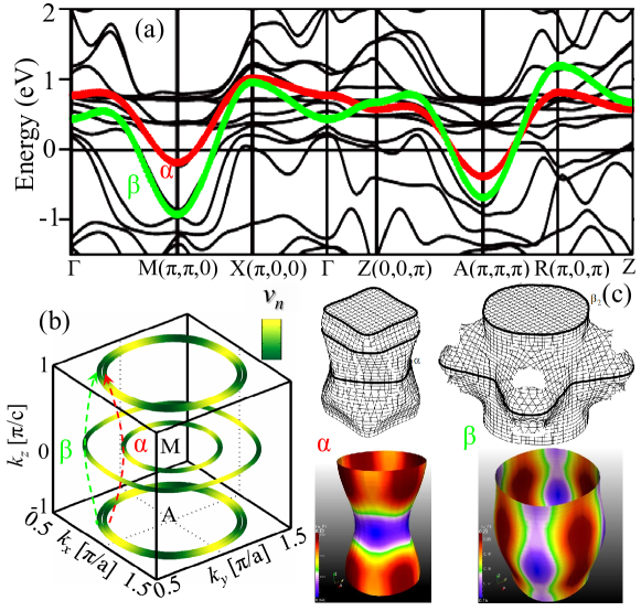
Figure 1: (color online) Electronic structure of CeCoIn₅: (a) Tight-binding fits of the two most relevant bands $\alpha$ (red) and $\beta$ (green) to the electronic dispersions of CeCoIn₅ calculated in the local density approximation by Maehira et al.Maehira (b) $\alpha$ and $\beta$ FSs at three representative $k_{z}$ values, colored by corresponding Fermi velocity from low (green) to high (yellow). (c) Three dimensional rendering of the computed FSs for $\alpha$ and $\beta$ bands (bottom panel) compared with the dHvA experimentsShishido03 (top panel). The $\alpha$ FS has a narrow waist, while the $\beta$ FS has a belly. The color map of the calculated FSs gives the anisotropy of the magnitude of the Fermi velocities ranging from low (blue) to high (red).

II Electronic structure

First-principles calculations of CeCoIn₅ demonstrate that the bands crossing the Fermi level are dominated by strongly hybridized $4f$ electrons of the Ce atom with weak overlap coming from the $5p$ orbitals of the In atom.Maehira2003 ; Maehira In this work our basic aim is to parameterize the true shape of the FSs only, while the overall dispersion feature at higher energy is irrelevant for thermodynamic and transport properties. Therefore, we use an effective tight-binding model of the lowest energy of three $4f-$orbitals in a tetragonal lattice. As we are only interested in the eigenvalues and not the eigenvectors of each band, we absorb the orbital symmetry of contributing orbitals into the tight-binding hopping parameters, which makes all bands decoupled from each other. With this motivation we write the tight-binding dispersion including up to third nearest neighbor hopping on the $x-y$ plane and only nearest neighbor hopping along $c-$axis to obtain

$$\xi_{{\bm{k}}}=-2\sum_{i}(t_{i}c_{i}+t_{2i}c_{2i})-4t_{xy}c_{x}c_{y}-E_{F}.$$ (1)

Here $c_{\alpha i}=\cos{(\alpha k_{i})}$ with $i=x,y,z$. $E_{F}$ is the Fermi energy. We obtain the values of the tight-binding parameters after fitting to first-principles dispersions by Ref. Maehira, shown in Fig. 1(a): ($t_{x}$=$t_{y}$,$t_{z}$,$t_{2x}$=$t_{2y}$,$t_{xy}$,$E_{F}$)=(-0.12,-0.05,0,0.09,-0.55), and (-0.17,0.06,0,0.15,-0.47) in eV for the $\alpha$ and $\beta$ band, respectively. Note that $t_{2z}=0$. The other two bands crossing the Fermi level have small areas and are not further considered in our two-band model description of CeCoIn₅.

The $\alpha$ and $\beta$ bands give two concentric electron pockets at the zone corner ($M$-point), see Fig. 1(b). The $k_{z}$ dispersion of each band is more interesting and needs special attention. Along the $k_{z}$ direction, both $\alpha$ and $\beta$ FSs are more like corrugated cylinders: the $\alpha$ FS has a narrow waist at $k_{z}=0$, while the $\beta$ FS has a belly. Note that only nearest neighbor hopping along the $c$ axis is sufficient to obtain the qualitative $k_{z}$ dispersion of all bands in agreement with the ab-initio band structureShishido and dHvA experimentsShishido03 [see Fig. 1(c)]. The opposite sign of the $t_{z}$ parameter is responsible for the opposite shape of the $\alpha$ and $\beta$ FSs (narrow waist vs. belly).

III Theory and computational method

For magnetic field ${{\bm{H}}}$ applied at angle $\alpha$ with respect to the (100) direction, we compute the field-angle induced superconducting DOS per spin, $N_{n}(\omega;{{\bm{H}}})$ (band index $n=1,2$) by solving the Eilenberger equation Anton ; Anton2010 ; AntonI ; AntonII within the extended BPT quasiclassical approximation. BPT ; WPesch1975 ; AHoughton1998 The BPT approximation implies a uniform field ${{\bm{H}}}$ over the unit cell of the Abrikosov vortex lattice (unit-cell averaged Green’s function). This produces quantitatively correct results near the upper critical field, and continues to yield semi-quantitatively correct description over the range $0.5H_{c2}(T)\lesssim H\leq H_{c2}(T)$ for isotropic gap, BPT ; Brandt ; Delireu and to much lower fields for nodal and strongly anisotropic gaps in single-band models.Vekhter99 ; TDahm2002 ; Anton

Here we summarize the key steps of the calculation, and highlight the main technical differences between the single- and multi-band systems following Refs. AntonI, ; AntonII, ; Anton2010, . The main object of interest, the quasiclassical Green’s function, is assumed to be diagonal in the band space ($n=1,2$), since bands are well separated in the Brillouin Zone, and have the 4$\times$4 Gor’kov-Nambu matrix structure corresponding to singlet pairing in each band,

$$\hat{G}=\left(\begin{array}[]{cc}\hat{g}_{1}&0\\ 0&\hat{g}_{2}\end{array}\right)\quad,\quad\hat{g}_{n}=\left(\begin{array}[]{cc}g_{n}&i\sigma_{2}f_{n}\\ i\sigma_{2}\underline{f}_{n}&-g_{n}\end{array}\right)\,.$$ (2)

The Green’s function in each band satisfies the Eilenberger equation for given Matsubara frequency $i\omega_{\nu}=i\pi T(2\nu+1)$, which has a simple commutator form:Serene1983

$$\Big{[}(i\omega_{\nu}+{e\over c}{\bm{v}}_{n}({\bm{k}}_{f})\cdot{{\bm{A}}}({\bm{R}}))\,\hat{\tau}_{3}-\hat{\Delta}_{n}({\bm{R}},{\bm{k}}_{f})-\hat{\sigma}^{imp}_{n}(i\omega_{\nu}),\,\hat{g}_{n}({\bm{R}},{\bm{k}}_{f};i\omega_{\nu})\Big{]}+i{\bm{v}}_{n}({\bm{k}}_{f})\cdot\bm{\nabla}_{\bm{R}}\;\hat{g}_{n}({\bm{R}},{\bm{k}}_{f};i\omega_{\nu})=0\,,$$ (3)

where the Fermi velocity in band $n$ is denoted by ${\bm{v}}_{n}({{\bm{k}}_{f}})$, with the wavevector ${\bm{k}}_{f}$ on the respective FS. Since this is a homogeneous equation, it has to be complemented by the normalization condition of the Green’s functions:

$$\hat{g}_{n}({\bm{R}},{\bm{k}}_{f};i\omega_{\nu})^{2}=-\pi^{2}.$$ (4)

Furthermore, the off-diagonal Green’s functions and self-energies are related by symmetry:Serene1983 $\underline{f}_{n}({\bm{R}},{\bm{k}}_{f};i\omega_{\nu})=f_{n}({\bm{R}},-{\bm{k}}_{f};i\omega_{\nu})^{*}=f_{n}({\bm{R}},{\bm{k}}_{f};-i\omega_{\nu})^{*}$; $\underline{\Delta}_{n}^{imp}({\bm{R}},{\bm{k}}_{f};i\omega_{\nu})=\Delta_{n}^{imp}({\bm{R}},-{\bm{k}}_{f};i\omega_{\nu})^{*}=\Delta_{n}^{imp}({\bm{R}},{\bm{k}}_{f};-i\omega_{\nu})^{*}$.

The equations for the Green’s functions in two bands are coupled indirectly through the self-energies entering the Eilenberger equation. The scattering of quasiparticles off impurities with concentration $n_{imp}$ is taken into account via the self-energy in each band, $\hat{\sigma}^{imp}_{n}$, which is evaluated in the $T$-matrix approximation for the two-band system,Ohashi ; Mishra2009

$$\hat{\sigma}^{imp}_{n}\equiv\left(\begin{array}[]{cc}D+\Sigma^{imp}_{n}&i\sigma_{2}\Delta^{imp}_{n}\\ i\sigma_{2}\underline{\Delta}^{imp}_{n}&D-\Sigma^{imp}_{n}\end{array}\right)=n_{imp}\hat{t}_{nn}\;,\qquad\hat{T}=\hat{U}+\hat{U}\langle N_{f}({\bm{k}}_{f})\hat{G}({\bm{k}}_{f})\rangle_{FS}\hat{T}.$$ (5)

The $\hat{T}$ matrix and the impurity scattering potential have the following structure in band space:

$$\hat{T}=\left(\begin{array}[]{cc}\hat{t}_{11}&\hat{t}_{12}\\ \hat{t}_{21}&\hat{t}_{22}\end{array}\right),\qquad\hat{U}=\left(\begin{array}[]{cc}u_{11}&u_{12}\\ u_{21}&u_{22}\end{array}\right).$$ (6)

The angular brackets denote the integral over one or the other Fermi surface, as appropriate, e.g.:

$$\langle\;N_{f}({\bm{k}}_{f})\,\hat{G}({\bm{k}}_{f})\;\rangle_{FS}=\mbox{diag}_{n=1,2}\left[\int_{FS_{n}}d^{2}k_{f}\;N_{f,n}({\bm{k}}_{f})\,\hat{g}_{n}({\bm{k}}_{f})\right]\,,$$ (7)

and the corresponding normal-state DOS at the Fermi level is $N_{f,n}({\bm{k}}_{f})\sim 1/|{\bm{v}}_{n}({\bm{k}}_{f})|$. Sometimes we will omit the subscript $FS$ for brevity.

For each $T$ and ${\bm{H}}$ the order parameters are calculated self-consistently from the coupled gap equations of the two-band model

$$\Delta_{n}({\bm{R}},{{\bm{k}}_{f}})=T\sum_{\omega_{\nu}}\sum_{m}\Big{\langle}V_{nm}({{\bm{k}}_{f}},{{\bm{k}}_{f}}^{\prime})\;N_{f,m}({{\bm{k}}_{f}}^{\prime})\,f_{m}({\bm{R}},{{\bm{k}}_{f}}^{\prime};i\omega_{\nu})\Big{\rangle}_{FS}.$$ (8)

We use a factorized pairing potential at the Fermi surface as $V_{nm}({{\bm{k}}_{f}},{{\bm{k}}_{f}}^{\prime})=V_{nm}\;{\cal Y}_{n}(\phi)\,{\cal Y}_{m}(\phi^{\prime})$, with ${\cal Y}_{n}(\phi)$ the basis function that depends only on the azimuthal angle, see Figs. 2 and 3. This means that the order parameters are also factorized, $\Delta_{1,2}({\bm{k}}_{f})=\Delta_{1,2}{\cal Y}_{1,2}(\phi)$. We couple the bands, for simplicity, by purely interband pairing $V_{12}=V_{21}=-V$, and assume same symmetries and angular variations on both bands ${\cal Y}_{1}(\phi)={\cal Y}_{2}(\phi)$. This ensures that the order parameters in the two bands are strongly coupled, and the temperature and field dependence of both gaps is similar, while keeping the number of parameters minimal. While there are indications that in CeCoIn₅ there is a small excitation gap that closes at very low fields, of order 0.1% of the upper critical field,Seyfarth it seems likely that this gap is proximity induced on the parts of the Fermi surface with low $f$-electron content that we do not consider here. Since all the experiments measuring the field-angle anisotropy are carried out at fields, which are at sufficiently high $H/H_{c2}$, we consider only Fermi surface sheets with strong pairing and large gaps. It is worth mentioning that the interband pairing captures both nodeless $s^{\pm}$ and nodal $d$ wave pairing scenarios.

Generally, for arbitrary interaction matrix $V_{nm}$, the coupled gap equations support two solutions for the amplitudes $(\Delta_{1},\Delta_{2})$. The physical solution corresponds to the highest transition temperature $T_{c0}$, that is, the greatest eigenvalue $V_{max}$ of the interaction matrix,

$$\left(\begin{array}[]{cc}V_{11}\langle N_{f,1}{\cal Y}_{1}^{2}\rangle&V_{12}\langle N_{f,2}{\cal Y}_{2}^{2}\rangle\\ V_{21}\langle N_{f,1}{\cal Y}_{1}^{2}\rangle&V_{22}\langle N_{f,2}{\cal Y}_{2}^{2}\rangle\end{array}\right)\left(\begin{array}[]{c}e_{1}\\ e_{2}\end{array}\right)=V_{max}\left(\begin{array}[]{c}e_{1}\\ e_{2}\end{array}\right)\,.$$ (9)

The effective interaction strength $V_{max}$ and the cutoff $\Omega_{c}$ can be eliminated using standard techniques in favor of the bare transition temperature, $T_{c0}=1.13\Omega_{c}\exp(-1/V_{max})$, Serene1983 and the gap amplitudes in different bands are given by the eigenvector of the interaction matrix,

$$\left(\begin{array}[]{c}\Delta_{1}\\ \Delta_{2}\end{array}\right)=\left(\begin{array}[]{c}e_{1}\\ e_{2}\end{array}\right)\Delta\>.$$ (10)

Upon projecting out this vector from Eq. (8), the system of the self-consistency equations is reduced to a single equation for the order parameter $\Delta$ of the dominant instability.

Since the only coupling between bands is via the self-consistency equations of the order parameter and the self-energies, the solutions for the propagators in each band can be formally obtained from the transport equation (3) with given $\Delta_{n}$ and $\sigma_{n}$ in the same way as for single-band systems.AntonI ; AntonII We express the gradient term via the raising and lowering operators $(a^{\dagger},a)$ for the vortex solutions corresponding to the superposition of different harmonic oscillator functions:AHoughton1998 ${\bm{v}}_{n}({\bm{k}}_{f})\cdot\left(\bm{\nabla}_{\bm{R}}-i\frac{2e}{c}{\bm{A}}({\bm{R}})\right)=\frac{1}{\sqrt{2}\Lambda}\,\left(v_{n,-}({\bm{k}}_{f})a^{\dagger}-v_{n,+}({\bm{k}}_{f})a\right).$ The $(x,y)$ projections of the Fermi velocity on the plane perpendicular to the direction of the field $\hat{z}$ have to be rescaled by the anisotropy factor $S_{f}$,

$$v_{n,\pm}=v_{n,x}({\bm{k}}_{f})/\sqrt{S_{f}}\pm iv_{n,y}({\bm{k}}_{f})\sqrt{S_{f}}.$$ (11)

The relevant parameter that determines the excitations in the SC state at a particular point on the Fermi surface is the component of the (rescaled) Fermi velocity normal to the applied field,

$$v_{n}^{\perp}({\bm{k}}_{f})=\sqrt{v_{n,x}({\bm{k}}_{f})^{2}/S_{f}+v_{n,y}({\bm{k}}_{f})^{2}\,S_{f}}.$$ (12)

The corresponding energy scale is

$$\bm{\bar{v}}_{f,n}(\phi,{{\bm{H}}})\equiv\frac{{{\bm{v}}}_{n}^{\perp}({{\bm{k}}_{f}})}{2\Lambda},$$ (13)

where $\Lambda=(\hbar c/2|e|H)^{1/2}$ is the magnetic length, which is of order of the intervortex distance, and $\phi$ is the FS angle with respect to the $k_{x}$ axis. The anisotropy parameter $S_{f}$ is chosen to give the correct form of the vortex lattice in the linearized Ginzburg-Landau (GL) equations for $\Delta$. This allows us to consider only the lowest Landau level,AntonI

$$\Delta({\bm{R}})=\Delta\sum_{k_{y}}C_{k_{y}}^{(n)}{e^{ik_{y}\sqrt{S_{f}}y}\over\sqrt[4]{S_{f}\Lambda^{2}}}\;\Phi_{0}\left({x-\Lambda^{2}\sqrt{S_{f}}k_{y}\over\Lambda\sqrt{S_{f}}}\right)\,.$$ (14)

For tetragonal symmetry this parameter depends on the angle that the applied field makes with the symmetry axis $c$ (in this paper $\theta_{H}=\pi/2$),

$$S_{f}=\sqrt{\cos^{2}\theta_{H}+{K_{||}\over K_{\perp}}\sin^{2}\theta_{H}}\,.$$ (15)

Here $K_{||}$ (along $c$-axis) and $K_{\perp}$ (in-plane) are the coefficients of the gradient terms in the GL expansion for the gradients along the $c$-axis and in the $ab$-plane respectively. For our two-band system they depend on the degree of mixing of the bands in a particular superconducting state $\Delta$. For the state $(\Delta_{1},\Delta_{2})=(e_{1}\Delta,e_{2}\Delta)$ they are determined by the right, $\vec{e}=(e_{1},e_{2})^{T}$, and left, $\vec{e^{\prime}}=(e_{1}^{\prime},e_{2}^{\prime})$, eigenvectors of the interaction matrix in Eq. (9), corresponding to eigenvalue $V_{max}$ with $\vec{e^{\prime}}\cdot\vec{e}=1$.

$$K_{||}=\frac{(e^{\prime}_{1}\,,\,e^{\prime}_{2})}{V_{max}}\left(\begin{array}[]{cc}V_{11}&V_{12}\\ V_{21}&V_{22}\end{array}\right)\left(\begin{array}[]{c}e_{1}\,\langle v_{1c}^{2}\,N_{f1}{\cal Y}_{1}^{2}\rangle\\ e_{2}\,\langle v_{2c}^{2}\,N_{f2}{\cal Y}_{2}^{2}\rangle\end{array}\right),$$ (20)

$$K_{\perp}=\frac{(e^{\prime}_{1}\,,\,e^{\prime}_{2})}{V_{max}}\left(\begin{array}[]{cc}V_{11}&V_{12}\\ V_{21}&V_{22}\end{array}\right)\left(\begin{array}[]{c}e_{1}\,\langle v_{1a}^{2}\,N_{f1}{\cal Y}_{1}^{2}\rangle\\ e_{2}\,\langle v_{2a}^{2}\,N_{f2}{\cal Y}_{2}^{2}\rangle\end{array}\right).$$ (25)

With these remarks in mind, we can directly use the single-band results for the unit-cell averaged Green’s functions in the single Landau level approximation [we follow the notation of Eqs. (46)-(48) in Ref. AntonI, ]:

$$g_{n}(i\omega_{\nu},{{\bm{k}}_{f}};{{\bm{H}}})=\frac{-i\pi}{\sqrt{1-i\sqrt{\pi}\frac{1}{\bar{v}_{f,n}^{2}}W^{\prime}\left(\frac{i\tilde{\omega}_{\nu,n}}{\bar{v}_{f,n}}\right)\tilde{\Delta}_{n}\underline{\tilde{\Delta}}_{n}}},$$ (26)

$$f_{n}(i\omega_{\nu},{{\bm{k}}_{f}};{{\bm{H}}})=ig_{n}\frac{\sqrt{\pi}}{\bar{v}_{f,n}}W\left(\frac{i\tilde{\omega}_{\nu,n}}{\bar{v}_{f,n}}\right)\tilde{\Delta}_{n}.$$ (27)

Here $i\tilde{\omega}_{\nu,n}=i\omega_{\nu}-\Sigma^{imp}_{n}(i\omega_{\nu},{\bm{k}}_{f};{\bm{H}})$ and $\tilde{\Delta}_{n}=\Delta_{n}({\bm{k}}_{f})+\Delta^{imp}_{n}(i\omega_{\nu},{\bm{k}}_{f};{\bm{H}})$ are the Matsubara frequency and the order parameter renormalized by the impurity self-energies in each band $n$, $\hat{\sigma}^{imp}_{n}$. $W^{\prime}(z)$ is the first derivative of the complex-valued function $W(z)=\exp{(-z^{2})}{\rm erfc}(-iz)$. One can further cast this in a form similar to that of a uniform superconductor by introducing the new self-energy $\Sigma_{n}$ according to $i\sqrt{\pi}/{\bar{v}_{f,n}^{2}}\;W_{n}^{\prime}(i\tilde{\omega}_{\nu}/\bar{v}_{f,n})\equiv(i\omega_{\nu}-\Sigma_{n})^{-2}$. The effective self-energy $\Sigma_{n}$ now contains effects from both the impurity scattering and the effects of orbital magnetic field.

In contrast to the Doppler shift approximation, both the real and the imaginary parts of $\Sigma_{n}$ contribute to the SC DOS, and their interplay as a function of energy, ${\bm{H}}$ and $T$, determine the sign reversal in the fourfold oscillation of the SC DOS. These effects have been extensively studied earlier using a single quasi-cylindrical FS and nodal gap, and a minimal 2D model for two-band systems, see for example Refs. Anton, ; AntonI, ; AntonII, ; Anton2010, .

The transport and thermodynamic coefficients are calculated by using the retarded Green’s functions through analytic continuation, $i\omega_{\nu}\to\omega+i0$, in the propagators found above. We begin with the total electronic specific heat from both bands, $C=C_{1}+C_{2}$, which is given by the derivative of the net entropy, $C=T\left(\partial S/\partial T\right)$. Because the low-temperature approximation given byAntonI

$$C_{n}(\alpha)\approx 2\int_{-\infty}^{\infty}d\omega\frac{\omega^{2}\langle N_{n}(\omega,{{\bm{k}}_{f}};{{\bm{H}}})\rangle_{FS}}{4T^{2}{\rm cosh}(\omega/2T)^{2}}\,,$$ (28)

remains valid almost up to the normal-state transition region, it can be employed to describe the behavior of the heat capacity over most of the phase diagram. Detailed numerical calculations show that the high-temperature sign reversal line is robust, but will be shifted to slightly higher temperatures by approximately $0.1T_{c0}$ for the FS parametrization considered here compared to the calculations using the low-temperature approximation in Eq. (28).

Next, we consider the total electronic thermal conductivity, which is the sum of the contributions from both bands, $\kappa=\kappa_{1}+\kappa_{2}$, with Vekhter99 ; AntonII

$$\kappa_{n}^{xx}(\alpha) = 2\int_{-\infty}^{\infty}\!\!d\omega\frac{\omega^{2}}{2T^{2}{\rm cosh}(\omega/2T)^{2}}$$

$$\times{\langle v_{n}^{x}({{\bm{k}}_{f}})^{2}N_{n}(\omega,{{\bm{k}}_{f}};{{\bm{H}}})\tau_{n}(\omega,{{\bm{k}}_{f}};{\bm{H}})\rangle_{FS}}\,.$$

Here the field-induced SC DOS per spin in each band, $N_{n}(\omega,{{\bm{k}}_{f}})/N_{f,n}({{\bm{k}}_{f}})=-{\rm Im}\ g^{R}(\omega,{{\bm{k}}_{f}};{{\bm{H}}})_{n}/\pi$, the factor $2$ accounts for the spin degeneracy, and the transport lifetime is due to both impurity and vortex scattering Vekhter99 ; AntonII ; Anton2010

$$\frac{1}{2\tau_{{n}}(\omega,{{\bm{k}}_{f}};{\bm{H}})}=-{\rm Im}\,\Sigma^{imp}_{n}(\omega,{{\bm{k}}_{f}};{{\bm{H}}})+\sqrt{\pi}{1\over|{\bar{{\bm{v}}}}_{f,n}({{\bm{k}}_{f}};{{\bm{H}}})|}\frac{{\rm Im}\,[g^{R}_{n}(\omega,{{\bm{k}}_{f}};{{\bm{H}}})\,W(\tilde{\omega}/|{\bar{{\bm{v}}}}_{f,n}({{\bm{k}}_{f}};{{\bm{H}}})|)]}{{\rm Im}\,g^{R}_{n}(\omega,{{\bm{k}}_{f}};{{\bm{H}}})}|\tilde{\Delta}_{n}({{\bm{k}}_{f}};{{\bm{H}}})|^{2}\,.$$ (30)

When $T\rightarrow 0$ we recover the standard expressions for the Sommerfeld coefficient, $\gamma_{n}\equiv C_{n}/T\to{2\over 3}\pi^{2}\langle N_{n}(0,{{\bm{k}}_{f}};{{\bm{H}}})\rangle_{FS}$, and for the linear coefficient of the thermal conductivity $\kappa_{n}^{xx}/T\to{1\over 3}\pi^{2}\langle v_{n}^{x}({{\bm{k}}_{f}})^{2}N_{n}(0,{{\bm{k}}_{f}};{{\bm{H}}})\tau_{n}(0,{{\bm{k}}_{f}};{\bm{H}})\rangle_{FS}$. Since the Green’s function, given by Eq. (26), takes the standard BCS form at $H=0$, we also recover the universal thermal conductivity for gaps with nodes on the FS.Sun1995 ; Graf1996 ; Graf1997 ; Norman1996 ; Graf1999 At low fields the approximation breaks down, but for nodal superconductors it provides a good interpolation from low to high fields, and, in the regime $1\ll 1/\tau_{imp}\Delta_{n}\ll H/H_{c2}$ reproduces the well-known $\sqrt{H}$ field-dependence of the density of states in $d$-wave superconductors Volovik1993 ; Kuebert98 up to logarithmic corrections.Vekhter99 ; AntonI ; AntonII

Since the function $x^{2}/{\rm cosh}(x/2)^{2}$ peaks at $x\sim 2.5T$, the anisotropy of the heat capacity at low temperatures is qualitatively determined by the anisotropy in the total SC DOS, $N(\omega=2.5T,{{\bm{k}}_{f}};{{\bm{H}}})$. Using the expansion of the error function, we obtain two limiting values for $W^{\prime}(z)$: $W^{\prime}(0)=2i/\sqrt{\pi}$ and $W^{\prime}(z\gg 1)\approx-i/\sqrt{\pi}z^{2}$. Thus the SC DOS for each band $n$ becomes

$$N_{n}(\omega;{{\bm{H}}})=\langle N_{n}(\omega,{{\bm{k}}_{f}};{{\bm{H}}})\rangle_{FS}\approx\begin{cases}\left\langle N_{f,n}({{\bm{k}}_{f}})\left[1+2\left(\frac{\widetilde{\Delta}_{n}({{\bm{k}}_{f}};{{\bm{H}}})}{|\bar{{\bm{v}}}_{f,n}({{\bm{k}}_{f}};{{\bm{H}}})|}\right)^{2}\right]^{-1/2}\right\rangle_{FS},&\omega\ll\bar{{\bm{v}}}_{f,n},\cr\left\langle N_{f,n}({{\bm{k}}_{f}})\left[1-\left(\frac{\widetilde{\Delta}_{n}({{\bm{k}}_{f}};{{\bm{H}}})}{\widetilde{\omega}}\right)^{2}\right]^{-1/2}\right\rangle_{FS},&\omega\gg\bar{{\bm{v}}}_{f,n}.\cr\end{cases}$$

(31)

The first line in Eq. (31) only makes physical sense when the BPT approximation is valid at low energies, i.e., for nodal and strongly anisotropic gaps. In that case at low $T$ (low energy) and low fields, where $\Delta_{n}({{\bm{k}}_{f}};{{\bm{H}}})$ only weakly depends on the direction of the field, the SC DOS depends predominantly on the orientation of ${\bar{{\bm{v}}}}_{f,n}({{\bm{k}}_{f}};{{\bm{H}}})$ relative to the minima of $\Delta_{n}({{\bm{k}}_{f}};{{\bm{H}}})$. At $\omega=0$ the inversion of the SC DOS as a function of the field for nodal gaps can be obtained in analogy with Refs. UdagawaI, ; AntonI, .

At higher energies, the second line of Eq. (31) has the BCS form apart from the replacement of the bare energies and gaps by their impurity renormalized counterparts. Therefore the field-angle variation enters via the anisotropy of these self-energies as well as via the field dependence of the gaps, $\Delta_{n}({{\bm{k}}_{f}};{{\bm{H}}})$, for determining the anisotropy of the upper critical field. The latter effect is only relevant in the vicinity of the transition to the normal state, where the result is valid for both nodal and nodeless gaps, including the fully isotropic situation. Crucially, for anisotropic Fermi surfaces the anisotropy in the self-energies and the order parameter is weighted by the normal-state angle-dependent DOS, $N_{f,n}({{\bm{k}}_{f}})$, leading to a complex behavior including the switching of the minima and maxima found in this work. However, in this regime the energy width of the Fermi weighting factor in the integral exceeds the gap amplitude and a full numerical evaluation is required. Our results are consistent with the general observations based on such an expansion.

For each pairing symmetry, the coupled order parameters are computed self-consistently at each temperature $T$ and for a given value of the magnetic field ${{\bm{H}}}$ applied at the angle $\alpha$ to the (100) direction. We calculate the field-angle oscillations in the $H$-$T$ phase diagram for a mesh of 35 field points between zero and $H_{c2}$, 100 temperature points from zero to $T_{c0}$, and 31 field-angle points $\alpha$ from zero to $90^{\circ}$ to extract the anisotropic terms in the heat capacity and thermal conductivity. For all the calculations, we consider purely intraband impurity scattering, $u_{12}=u_{21}=0$, $u_{11}=u_{22}=u_{0}$, in the clean limit, $2\Gamma_{1}=1/\tau_{imp,1}=2n_{imp}/\pi N_{f1}=0.01\times 2\pi T_{c0}$, where $T_{c0}$ is the bare transition temperature, $N_{f1}$ is the density of states on the first band ($\alpha$-band), and the scattering phase shift is chosen to be $\delta=\arctan(\pi N_{f1}u_{0})=\pi/2$ (unitarity limit).

IV Results

IV.1 Field-induced superconducting DOS anisotropy and the role of Fermi surface topology

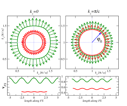
Figure 2: (color online) Fermi surfaces (FSs) and Fermi velocities at $k_{z}=0$ (left panel) and $k_{z}=\pi/c$ (right panel). The relative magnitude of the Fermi velocities (in arbitrary units) is given by the length of the (red and green) arrows in the top panels. The bottom panels show the Fermi velocities along the Fermi lines of the corresponding $k_{z}$ slice.

As discussed above, an important aspect influencing our results is that, for the realistic band structure, the contributions from different segments of the Fermi surfaces to the net density of states are weighted differently according to both the factor $N_{f,n}$ in Eq. (31), and the segment length of the Fermi surface with a given direction of the Fermi velocity. Fig. 2 shows the profiles of the Fermi velocity and the corresponding weighting factors. The key point is that, in a tetragonal system, ${\bm{v}}_{f,n}$ can have a fourfold anisotropy in the plane that either enhances or competes with the gap anisotropy in determining the contribution to the net DOS in the superconducting state, see Fig. 3(a). The detailed interplay of the two depends not only on the value of the angle-resolved DOS, but also on the direction of the Fermi velocity.

Indeed, naively one might expect that the relatively large contribution to $N_{f,n}$ from the near-45^∘ direction, combined with the node of the $d_{x^{2}-y^{2}}$ at the same angle in Fig. 3(a) should enhance the field-angle anisotropy for that symmetry of the superconducting state relative to the $d_{xy}$ case when the direction of the greatest $N_{f,n}$ is fully gapped. In fact, the opposite is true, see Fig. 3(b): the oscillations are enhanced for $d_{xy}$ symmetry.

This is an indication that the flat parts of the Fermi surface with large values of the Fermi velocity, see Fig. 2, contribute more to the total DOS, when the field is at $45^{\circ}$ and all four flat parts are ’active’. When the field is along $0^{\circ}$ or $90^{\circ}$, only two flat parts contribute. In contrast, the four ’active’ corners with smaller velocities, and hence slightly larger $N_{f,n}({\bm{k}}_{f})$ give a smaller contribution simply because their arc length is a smaller fraction of the total Fermi surface length in the respective $k_{z}$ slice. It follows that $d_{xy}$-pairing, which has nodes in the flat parts of the FS, exhibits enhanced $C(\alpha=45^{\circ})$. In contrast, the $d_{x^{2}-y^{2}}$ profile, gaps those regions of the Fermi surface and thus anisotropy of $C$ is suppressed. Hence the exact role of the Fermi surface shape and curvature in the field-angle oscillations is highly non-trivial.

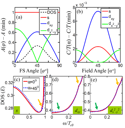
Figure 3: (color online) Fermi surface anisotropy of the normal-state DOS and SC gaps contrasted with the field-angle anisotropy of the Sommerfeld coefficient and the SC DOS. (a) The calculated FS anisotropy of the normal-state DOS juxtaposed with gap functions of three pairing symmetries. All the SC gaps are computed at the FS and all curves are shifted by their corresponding minimum value, except for the $s$-wave gap. (b) Specific heat coefficient $\gamma(\alpha)=C(\alpha)/T$, normalized to its value at $T_{c}$, calculated at $T/T_{c0}=0.1$ and $H/H_{c2}=0.1$ for $d$-wave gaps and $H/H_{c2}=0.5$ for the $s$-wave gap. (c)-(e) Field-induced total SC DOS at $T=0$ vs.  energy at two representative field angles $\alpha=0^{\circ}$ and $45^{\circ}$ for all three pairing symmetries. Here we used $H/H_{c2}=0.5$ for $s$ wave and 0.1 for both $d$ waves. Note the low- and high-energy crossings in the SC DOS (arrows) are related to the low- and high-$T$ sign reversals in the oscillations of $\gamma$ and $\kappa$ in Fig. 4.

At higher temperatures the simple low-$T$ expression in Eq. (7) is only qualitatively correct, and both detailed calculations Anton ; AntonI ; UdagawaI ; MiranovicI and experiments An2010 ; FeSeTe_exp ; ceirin5 demonstrated that the anisotropy in the heat capacity is reversed relative to the low-$T$ result. The lower panel in Fig. 3 shows the field-induced SC DOS as a function of quasiparticle energy below the SC gap for $\alpha=0^{\circ}$ and $\alpha=45^{\circ}$ for all three pairing symmetries considered here. We immediately see that the SC DOS at these angles switch and reverse magnitude, which reflects in the sign reversal of the oscillations in specific heat as a function of temperature. Note that, due to the presence of Fermi velocities in $\kappa$ in Eq. (7), a one-to-one correspondence between SC DOS and $\kappa$ is not straightforward for FS that lack continuous rotational symmetry in the plane.

We show below that for realistic and material-specific anisotropic FS, we still find the sign reversal of the heat capacity oscillations for $d$-wave pairing, which was previously reported for the rotationally symmetric cases. Hence this sign change is a generic feature of of nodal gaps. However, the key finding in this work is that for moderately anisotropic FSs, measurably large field-angle dependence in the heat capacity and thermal conductivity is obtained at high fields already for isotropic gaps, which can lead to misinterpretations if analyzed solely in this field range and in terms of simple harmonics of the SC pairing symmetries. We stress that multiband effects add additional complexity to any analysis, due to competing FS anisotropies. For example, we have previously shown that if the FS anisotropy in different bands is opposite (out-of-phase) to each other, then it can lead to additional sign reversals in the field-angle dependence of the thermodynamic quantities for $s$-wave gap, very similar to what was earlier obtained for nodal gaps only.DasFeSe Furthermore, bands with different DOS lead to different amplitudes and shapes of the self-consistent value of the SC gaps (i.e., generally $\Delta_{1}\neq\Delta_{2}$). In this case, the obtained numerical results become less intuitive to interpret and a simple one-to-one mapping between oscillations and nodes is lost. However, at low temperature and low field the generic understanding of the anisotropy as a consequence of the nodal structure alone, remains valid. We give a detailed comparison of the different regimes below.

IV.2 Temperature evolution of field-angle-resolved oscillations

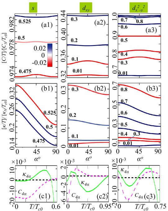
Figure 4: (color online) Calculated oscillations of the heat capacity and thermal conductivity as a function of the field direction relative to the $x$ axis. (a1) Sommerfeld coefficient $\gamma=C/T$ normalized to its normal-state value $C_{N}/T_{c0}$ at fixed field $H/H_{c2}=0.5$ for $s$ wave, plotted from low to high $T$ in units of $T/T_{c0}$ (bottom to top curves). Each curve is colored by the sign of the fourfold oscillation; a uniform color map is used for values below $-0.025$ and above $0.025$. (b1) Same as in (a1) but for the normalized thermal conductivity coefficient $\kappa/T$. (c1) The fourfold amplitudes of $\gamma$ (dashed line) and $\kappa/T$ (solid line) are plotted as a function of $T$. For direct comparison the results for nodal $d_{xy}$ ($H/H_{c2}=0.1$) and $d_{x^{2}-y^{2}}$ ($H/H_{c2}=0.33$) symmetries are plotted in panels (a2)-(a3), (b2)-(b3), and (c2)-(c3), respectively. Note that the non-vanishing of $\kappa_{4\alpha}$ as temperature approaches the phase transition line in panels (c1) and (c3) is a consequence of the in-plane anisotropy of $H_{c2}$.

We present the full angle-dependent profiles of $\gamma(\alpha)=C(\alpha)/T$ and $\kappa(\alpha)/T$ for several temperatures at a representative low field ($H/H_{c2}=0.1$) for the two nodal gaps, and, for comparison, for an isotropic $s$-wave gap at a moderate field ($H/H_{c2}=0.5$) in Fig. 4. In accordance with our earlier calculation for K_yFe_2-xSe₂ in Ref. DasFeSe, , we find that a substantial oscillation in $\gamma$ and $\kappa$ is present for isotropic $s$-wave pairing. The amplitude of the oscillation increases with stronger $k_{z}$-dispersion. As in simple models,AntonI close to the inversion line the oscillations are not a simple sum of the twofold and fourfold harmonics, but have a more complex profile.

For nodal $d_{xy}$ and $d_{x^{2}-y^{2}}$ pairings, the behavior of oscillations of $\gamma(\alpha)$ and $\kappa(\alpha)$ is similar to results obtained for quasicylindrical FSs, Anton2010 however the amplitude of oscillations and, crucially, the location of sign reversals in the $H$-$T$ phase diagram are modified. Earlier such sign-reversal features were discussed only for highly anisotropic or nodal gap structures.Anton ; AntonI ; Anton2010 ; An2010 ; FeSeTe_exp ; ceirin5 Our material-specific results caution against straightforward interpretation of oscillations at intermediate fields as evidence of nodes, emphasizing the need to probe low energy excitations.

We extract the amplitudes of the fourfold oscillations by defining

$$C_{4\alpha}(T)\equiv\Pi_{0}^{C}-\Pi_{45}^{C},$$ (32)

where $\Pi_{\alpha}^{C}=[C(\alpha,T)/T]/[C_{N}/T_{c}]$ and

$$\kappa_{4\alpha}(T)\equiv[\Pi_{0}^{\kappa}+\Pi_{90}^{\kappa}]/2-\Pi_{45}^{\kappa},$$ (33)

where $\Pi_{\alpha}^{\kappa}=[\kappa^{xx}(\alpha,T)/T]/[\kappa^{xx}_{N}/T_{c}]$, and $C_{N}$ and $\kappa_{N}$ are the corresponding normal-state values at $T_{c}$. This definition removes any twofold, sixfold, etc., contribution from $\kappa(\alpha)$ originating from the field parallel or perpendicular to the vortex lines.kappa In fact, it is straightforward to show that for any function $f(\alpha)=\sum_{n=0}^{M}a_{2n}\cos(2n\alpha)$ the definition in Eq. (33) projects out any other harmonic contribution up to $M=5$, resulting in $\kappa_{4\alpha}=2a_{4}$. We verified numerically that the amplitudes of twelvefold and higher order harmonics are negligible. On the other hand, the definition in Eq. (32) is less robust, but very convenient. It gives $C_{4\alpha}=2a_{4}$, when $a_{2}=a_{6}=a_{10}=0$, which is sufficient when sample misalignment is negligible and when used away from the sign reversal line.

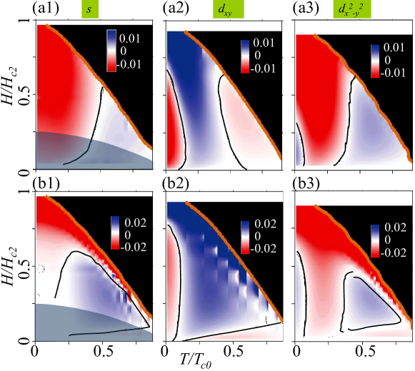
Figure 5: (color online) Contour maps of fourfold amplitude oscillations of normalized specific heat $C_{4\alpha}$ (row $a$) and normalized thermal conductivity $\kappa_{4\alpha}$ (row $b$) in the $H$-$T$ phase diagram. Each column denotes a different gap symmetry studied (isotropic nodeless $s$, nodal $d_{xy}$ and $d_{x^{2}-y^{2}}$ gaps). All plots use the same color map scale from minimum (red) to maximum (blue). Note that the fourfold amplitude is given with respect to field ${{\bm{H}}}\parallel(100)$, i.e., a negative value corresponds to a minimum at $\alpha=0^{\circ}$. Here $T_{c}({{\bm{H}}})$ is defined by the vanishing of both gaps for given symmetry, which determines the line of the (minimum) upper critical field. Since the BPT approximation for isotropic $s$-wave pairing is not valid at low $H$, we shaded the corresponding area where our approach is not applicable.

IV.3 $H$-$T$ phase diagram

In figure 5 we compile our results of the thermal quantities into a contour map of the amplitude of the fourfold oscillations in the $H$-$T$ phase diagram for $\gamma=C/T$ (top row) and $\kappa/T$ (bottom row) for one nodeless and two nodal gaps. Recall that for quasicylindrical (rotationally-invariant in the basal plane) FSs the specific heat oscillations simply change sign between the $d_{xy}$ and $d_{x^{2}-y^{2}}$ symmetries.AntonI While the overall characteristics of the phase diagram remains qualitatively the same for material-specific cases, substantial quantitative changes result from the inclusion of realistic Fermi surfaces and the directional- and band-dependent contributions to the DOS. Important for the comparison with experiment, we find that the location of the sign-reversal lines for nodal gaps shown in Figs. 5(a2) and 5(a3) shifted compared to the earlier simple models, due to the interplay of the SC order parameter with the FS anisotropies. As a consequence, the sign of the fourfold oscillations, $C_{4\alpha}$ and $\kappa_{4\alpha}$, may be different over a wider range of temperatures and fields. This is to be contrasted with the results for rotationally symmetric Fermi surfaces, where the two were found to switch sign almost at the same temperatures and fields. We also verified that for $s$-wave pairing the high-$T$ sign reversal is robust and remains at nearly the same location for a single-band superconductor with identical FS.

Note also that at intermediate to high temperatures and fields there is very little in the heat capacity oscillation profile that distinguishes the isotropic gap from that of the $d_{x^{2}-y^{2}}$ symmetry, see Fig. 5 panels (a1) vs. (a3). However, there is a much more significant difference in transport, Fig. 5 panels (b1) vs. (b3), which implies that a simultaneous study of both $C(\alpha)$ and $\kappa(\alpha)$ is highly desirable to gain confidence about the underlying pairing symmetry in any multiband system where the low-temperature, low-field regime is experimentally unreachable. Of course, once the low energy sector at low $T$ and low $H$ is accessed, the differences between different symmetries, and especially between the nodal and isotropic gaps, becomes obvious. Therefore, in general a rather detailed comparison between measurements and calculations of the $C_{4\alpha}$ and $\kappa_{4\alpha}$ phase diagrams should be employed to draw conclusions about the pairing symmetries.

IV.4 Comparison with experiments

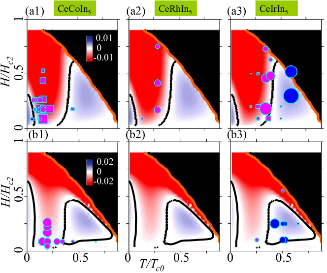
Figure 6: (color online) Theoretical contour maps of fourfold amplitude oscillations for $d_{x^{2}-y^{2}}$ gap for specific heat (upper panel), and thermal conductivity (lower panel) of CeCoIn₅, reproduced from Figs. 5(a3)-b(3). The same theoretical data is repeated in three columns, but compared with three different experimental data for isostructural superconductors within the Ce-115 family. (a1): Specific heat data of CeCoIn₅ by An et al.An2010 (circles) and Aoki et al.Aoki2004 (squares). (b1): Thermal conductivity data of CeCoIn₅ by Izawa et al.Izawa2001 (a2): Specific heat data for CeRhIn₅ by Park et al. Park2008 ; Park2009 (a3): Specific heat data for CeIrIn₅ by Lu et al.ceirin5 (circles) and Kittaka et al.Kittaka2012 (squares). (b3): Thermal conductivity data of CeIrIn₅ by Kashara et al. Kasahara2008 The symbol size gives the corresponding reported amplitude of the oscillation, whereas the filled color depicts its sign. We find reasonable agreement between theory and experiment in both sign and amplitude of oscillations.

The superconducting Ce-115 compounds are well suited for the study of field-angle oscillations. Accordingly, there have been a number of experiments investigating the anisotropy of the thermal conductivity and the heat capacity under the rotated field. Here we compare the experimental results with our findings, previously shown in Fig. 5. Since the upper critical field is Pauli-limited, and our calculation does not account for the Zeeman splitting, we cannot expect our results to map directly onto the measurements near $H_{c2}$. Nevertheless we believe that a qualitative comparison can be made, especially for systems with strong paramagnetism in the low-field part of the phase diagram, which, when rescaled to the appropriate values of the upper critical field, is essentially identical to that computed in the absence of the Zeeman term. Anton2010a

CeCoIn₅:  The unconventional nature of superconductivity was recognized early on through the discovery of power-law dependence in the temperature behavior of the specific heat and thermal conductivity,Petrovic2001a ; Movshovich2001 magnetic penetration depth, Ormeno2002 ; Chia2003 ; Ozcan2003 ; Bauer2006 and spin-lattice and muon-spin relaxation rates Kohori2001 ; Higemoto2002 consistent with predictions for nodal lines in the gap. On symmetry grounds the anisotropy of the upper critical field vanishes near $T_{c0}$, $H_{c2}(0^{\circ})=H_{c2}(45^{\circ})$. In our calculations, we find that noticeable anisotropy emerges for $T/T_{c0}\lesssim 0.7$. In this range $H_{c2}(0^{\circ})>H_{c2}(45^{\circ})$ for both $s$ and $d_{x^{2}-y^{2}}$ pairing symmetries, while the anisotropy is opposite for $d_{xy}$ pairing, i.e., the nodal directions have a lower $H_{c2}$ value. The anisotropy for $s$ and $d_{x^{2}-y^{2}}$ gap is in qualitative agreement with the $H_{c2}$ measurements of CeCoIn₅ by Settai et al.,Settai2001 who reported $H_{c2}(0^{\circ})>H_{c2}(45^{\circ})$ at low temperatures. The measured anisotropy is only a few percent, which would be consistent with the assumption that the band electron $g$-factor, and hence the Pauli limiting field is isotropic in the plane, and the weak anisotropy is due to a residual orbital effect. Remarkably, the opposite relationship, $H_{c2}(0^{\circ})=11.8\,{\rm T}<H_{c2}(45^{\circ})=11.9\,{\rm T}$ was found in Ref. Murphy2002, . So far the experimental discrepancy of the in-plane $H_{c2}$ anisotropy remains an open puzzle.

The original interpretations of the field-angle-resolved thermal conductivity Izawa2001 and specific heat Aoki2004 measurements contradicted each other regarding the location of the $d$-wave nodal lines in CeCoIn₅. The controversy was finally settled by the observation of the inversion in the specific heat oscillations by An et al.An2010 In Fig. 6(a1) and (b1) we plot both the $C_{4\alpha}$ and $\kappa_{4\alpha}$ experimental data points (symbols). The agreement between theory and experiment is quite convincing for $d_{x^{2}-y^{2}}$-wave symmetry and rules out pairing scenarios of either $s$ or $d_{xy}$ gap.

CeRhIn₅:  The high-pressure, angle-resolved specific heat measurements of CeRhIn₅ by Park et al.Park2008 showed a clearly delineated fourfold oscillation with $C(0^{\circ})<C(45^{\circ})$, which was interpreted in favor of $d$-wave symmetry. The measurements were performed down to temperatures as low as 0.3 K ($0.3T/T_{c}$) and in fields between 0.2 and 0.9 T. At the pressure of 1.47 GPa the superconductivity coexists with antiferromagnetism with superconducting transition $T_{c}=1.04$ K and in-plane $H_{c2}=1.2$ T at 0.3 K. The measured in-plane $H_{c2}$ anisotropy was negligible. As we noted before, in this region of the $H$-$T$ phase diagram both $s$-wave and $d_{x^{2}-y^{2}}$-wave gaps are nearly indistinguishable giving rise to fourfold oscillations with the minimum of $C(\alpha)$ occurring at ${{\bm{H}}}\parallel(100)$. Supporting the $d$-wave interpretation, $T$- and $H$-dependent measurements down to 0.3 K and 0.05 T exhibited power-law behavior consistent with unconventional superconductivity with nodes, i.e., $C/T\sim T$ and $C/T\sim\sqrt{H}$, respectively. Additional experiments at higher pressure (2.3 GPa), i.e., in the purely superconducting phase, and at $T/T_{c}=0.14$ and $H/H_{c2}=0.09$ showed evidence of fourfold oscillations with a negative amplitude $C_{4\alpha}$ of order 4%.Park2009 However, to unequivocally rule out the possibility of $s$-wave pairing, based on field-angle-resolved measurements alone, experiments would have to be performed at temperatures significantly below $T_{c}/3$, where the exponential $T$-dependence of the fully gapped excitation spectrum becomes visible. Power laws were also seen in other pressure measurements of the specific heat, spin-lattice and muon-spin relaxation rates down to $T/T_{c}\approx 0.15$.Phillips2002 ; Mito2001 ; Higemoto2002 In chemically doped CeRh_1-xIr_xIn₅ a $T^{3}$ dependence was seen in $1/T_{1}$ just below $T_{c}$, which tends toward linear in $T$ at lower temperatures as is typical of dirty $d$-wave superconductors.Kawasaki2006 In Fig. 6(a2) we plot the $C_{4\alpha}$ experimental data points (symbols) on top of the phase diagram for $d_{x^{2}-y^{2}}$ gap. The field-angle-dependent experiments taken by themselves are inconclusive, though combined with the reported $T$ and $H$ dependences are strongly suggestive of $d_{x^{2}-y^{2}}$-wave superconductivity in CeRhIn₅.

CeIrIn₅:  There is an ongoing controversy about the pairing symmetry in this compound, because of its two different superconducting domes, namely one as a function of Rh doping and the other as a function of pressure. In addition, there is disagreement over the interpretation of the thermal conductivity data. On one side, the field-angle-resolved measurements Kasahara2008 and power-law dependence in temperature were argued as evidence for $d$-wave gap with vertical line nodes, similar to the sister compound CeCoIn₅,Petrovic2001b ; Movshovich2001 while on the other side thermal conductivity measurements, in particular the temperature and magnetic field dependence of the residual value of $\kappa/T$ along different axes, were interpreted in favor of a three-dimensional hybrid gap with a horizontal line node. Shakeripour2007 ; Shakeripour2009 ; Shakeripour2010 The hybrid gap proposal was inspired by similar gap functions studied some time ago for the heavy-fermion superconductor UPt₃.Graf1997 ; Graf1999 ; Graf2000 To further complicate the interpretation, the results by Shakeripour et al. were also argued to be consistent with vertical line nodes.Vekhter2007 In addition, power laws were reported for magnetic penetration depth and spin-lattice-relaxation rate.Vandervelde2009 ; Kawasaki2006 ; Kohori2001 The temperature behavior of the anisotropic penetration depth was interpreted to be consistent with vertical line nodes but not with point nodes and a horizontal line node of the hybrid gap.Vandervelde2009 However, the conclusive evidence for the in-plane gap variation comes from very recent angle-resolved specific heat measurements at ambient and finite pressure. Lu et al. ceirin5 (circles) reported fourfold oscillations inside the pressure dome of CeIrIn₅ with sign reversal of the oscillations at high temperatures between 0.4 and $0.6T_{c}$. These data taken together with a low-$T$ anisotropy of $H_{c2}(0^{\circ})>H_{c2}(45^{\circ})$ and the fact that this compound belongs to the same family of Ce-115s was strongly suggestive of two-dimensional $d_{x^{2}-y^{2}}$-wave pairing with vertical line nodes. Unfortunately, the temperature in Ref. ceirin5, was too high to formally exclude isotropic $s$-wave pairing, see the phase diagram in Fig. 5(a1) versus (a3). The specific heat data of Ref. Kittaka2012, , on the other hand, were taken down to 80 mK, that is $0.2T_{c}$. Therefore, the specific heat oscillations are supportive of the $d_{x^{2}-y^{2}}$ gap scenario. Data from both experiments are included in the comparison in Fig. 6(a3). In addition field-angle-resolved thermal conductivity data were reported by Kasahara et al.,Kasahara2008 which are shown in Fig. 6(b3). Combined with the specific heat oscillations, they provide strong support for this pairing symmetry. Hence at present the overwhelming majority of experiments supports the $d_{x^{2}-y^{2}}$-wave superconductivity with vertical line nodes in CeIrIn₅.

V Discussion and Conclusions

We performed realistic model calculations of the field-angle-resolved specific heat and thermal conductivity using a tight-binding parametrization of the electronic structure within a two-band model of superconductivity, which is relevant for the Ce-115 heavy fermions. Our systematic analysis of field-angle dependence showed that modest anisotropies in the density of states and the in-plane Fermi velocities of a tetragonal crystal contributes significantly to the fourfold oscillations in the vortex state, when the magnetic field is rotated in the basal plane. As evidence we showed that such oscillations exist at intermediate to high fields even for an isotropic $s$-wave gap. Remarkably, the sign reversal of fourfold oscillations occurs not only for nodal $d$-wave gaps, but also for an isotropic $s$-wave gap as the temperature is decreased. This is one of the main findings of this work and implies that away from the low temperature and low field region it may be difficult to distinguish different pairing symmetries based on the field-anisotropy of a single probe alone.

Finally, we compared the results of the field-angle-resolved calculations within our model with recent experimental data on different members of the Ce-115 family. The behavior of the self-consistently determined thermal quantities for nodal $d_{x^{2}-y^{2}}$-wave gap is consistent with experimental reports for CeCoIn₅. The same phase diagram is also consistent with specific heat data for CeRhIn₅ and CeIrIn₅. Since both CeRhIn₅ and CeIrIn₅ have similar electronic structure as CeCoIn₅ near the Fermi energy, we believe that our Fermi surface parametrization is valid for all three compounds. Consequently, very similar phase diagrams should result for all three materials for which material-specific calculations drastically improved the agreement between theory and experiment. The comparison with experimental data is restricted to low fields, since the superconductivity in this material is Pauli-limited,Bianchi2003a ; Bianchi2003b and there are indications of a quantum critical point in the vicinity of the upper critical field at zero temperature, $H_{c2}(0)$.Bianchi2003 ; Paglione2003 Thus the regime near the upper critical field at low temperatures is beyond the scope of the current treatment. We find that within our realistic model of the Fermi surface parameters the fourfold anisotropy map is in better agreement with experiments on CeCoIn₅, if we assume a weak dispersion along the $k_{z}$ axis. Note that the relatively small anisotropy of the upper critical field in this material does not have direct connection with the anisotropy of the electron dispersion, as it likely stems from the Pauli limiting of superconductivity. Since the electronic band structure is very similar among the Ce-115s near the Fermi energy, we expect that our findings for CeCoIn₅ are also relevant for CeRhIn₅ and CeIrIn₅ under pressure. Considering that questions remain about the exact superconducting gap structure and potential spin-fluctuation nesting in the Ce-115s,Ronning2012 a definitive theoretical account of field-angle-resolved measurements is warranted.

We conclude with a note of caution for interpreting field-angle-resolved oscillations. Our self-consistent two-band model calculations demonstrated that simple observations of oscillations and sign reversals in either $C(\alpha)$ or $\kappa(\alpha)$ are not direct evidence for the presence of nodes or minima in the gap structure. Such conclusions can be drawn either from low-energy measurements, or at higher temperatures and field from a comprehensive simultaneous analysis within the same framework of both $C(\alpha)$ and $\kappa(\alpha)$ measurements. Only a systematic analysis of the fourfold oscillations in the $H$-$T$ phase diagram can constrain the space of possible pairing scenarios for a given material.

- (1) I. Vekhter, P. J. Hirschfeld, J. P. Carbotte, and E. J. Nicol, Phys. Rev. B 59, R9023 (1999).
- (2) P. Miranovic, M. Ichioka, K. Machida, and N. Nakai, J. Phys.: Condens. Matter 17, 7917 (2005).
- (3) A. B. Vorontsov and I. Vekhter, Phys. Rev. Lett 96, 237001 (2006).
- (4) Y. Matsuda, K. Izawa, and I. Vekhter, J. Phys.: Condens. Matter 18, R705 (2006).
- (5) T. Park, M. B. Salamon, E. M. Choi, H. J. Kim, and S. I. Lee, Phys. Rev. Lett. 90, 177001 (2003).
- (6) K. An, T. Sakakibara, R. Settai, Y. Onuki, M. Hiragi, M. Ichioka, and K. Machida, Phys. Rev. Lett. 104, 037002 (2010).
- (7) S. Kittaka, Y. Aoki, T. Sakakibara, A. Sakai, S. Naktsuji, Y. Tsutsumi, M. Ichioka, and K. Machida, Phys. Rev. B 85, 060505 (2012).
- (8) A. B. Vorontsov and I. Vekhter, Phys. Rev. B 75, 224501 (2007).
- (9) A. B. Vorontsov and I. Vekhter, Phys. Rev. B 75, 224502 (2007).
- (10) I. Vekhter and A. B. Vorontsov, Physica B 403, 958(2008)
- (11) T. Das, A. B. Vorontsov, I. Vekhter, and M. J. Graf, Phys. Rev. Lett. 109, 187006 (2012).
- (12) K. Izawa, H. Yamaguchi, Y. Matsuda, H. Shishido, R. Settai, and Y. Onuki, Phys. Rev. Lett. 86, 2653 (2001).
- (13) H. Aoki, T. Sakakibara, H. Shishido, R. Settai, Y. Onuki, P. Miranovic, and K. Machida, J. Phys.: Condens. Matter 16, L13 (2004).
- (14) A. Bianchi, R. Movshovich, N. Oeschler, P. Gegenwart, F. Steglich, J. D. Thompson, P. G. Pagliuso, and J. L. Sarrao, Phys. Rev. Lett. 89, 137002 (2002).
- (15) A. Bianchi, R. Movshovich, C. Capan, P. G. Pagliuso, and J. L. Sarrao, Phys. Rev. Lett. 91, 187004 (2003).
- (16) A. Bianchi, R. Movshovich, I. Vekhter, P. G. Pagliuso, and J. L. Sarrao, Phys. Rev. Lett. 91, 257001 (2003).
- (17) J.-P. Paglione, M. A. Tanatar, D. G. Hawthorn, E. Boaknin, R. W. Hill, F. Ronning, M. Sutherland, and L. Taillefer, Phys. Rev. Lett. 91 246405 (2003).
- (18) F. Ronning, J.-X. Zhu, T. Das, M. J. Graf, R. C. Albers, H. Rhee, W. E. Pickett, J. Phys.: Condens. Matter 24, 294206 (2012).
- (19) T. Maehira, T. Hotta, K. Ueda, and A. Hasegawa, Phys. Rev. Lett. 90, 207007 (2003).
- (20) H. Shishido, T. Ueda, S. Hashimoto, T. Kubo, R. Settai, H. Harima, and Y. Onuki, J. Phys.: Cond. Mat. 15, L499 (2003).
- (21) T. Maehira, T. Hotta, K. Ueda, and A. Hasegawa, J. Phys. Soc. Jpn. 72, 854 (2003).
- (22) H. Shishido et al., J. Phys. Soc. Jpn. 71, 162 (2002).
- (23) A. B. Vorontsov and I. Vekhter, Phys. Rev. Lett 105, 187004 (2010).
- (24) U. Brandt, W. Pesch, and L. Tewordt, Z. Phys. 201, 209 (1967).
- (25) W. Pesch, Z. Phys. B 21, 263 (1975).
- (26) A. Houghton and I. Vekhter, Phys. Rev. B 57, 10831 (1998).
- (27) E. H. Brandt, J. Low Temp. Phys. 24, 409 (1976).
- (28) J. M. Delrieu, J. Low Temp. Phys. 6, 197 (1972).
- (29) I. Vekhter and A. Houghton, Phys. Rev. Lett. 83, 4626 (1999).
- (30) T. Dahm, S. Graser, C. Iniotakis, and N. Schopohl, Phys. Rev. B 66, 144515 (2002).
- (31) J. W. Serene and D. Rainer, Physics Reports 101, 221 (1983).
- (32) Y. Ohashi, Physica C 412-414, 41 (2004).
- (33) V. Mishra, A. Vorontsov, P. J. Hirschfeld, and I. Vekhter, Phys. Rev. B 80, 224525 (2009).
- (34) G. Seyfarth, J. P. Brison, G. Knebel, D. Aoki, G. Lapertot, and J. Flouquet, Phys. Rev. Lett. 101, 046401 (2008)
- (35) Y. Sun and K. Maki, Europhys. Lett. 32, 355 (1995).
- (36) M. J. Graf, S.-K. Yip, J. A. Sauls, and D. Rainer, Phys. Rev. B 53, 15147 (1996).
- (37) M. J. Graf, S.-K. Yip, and J. A. Sauls, J. Low Temp. Phys. 102, 367 (1996); Erratum: 106, 727 (1997).
- (38) M. R. Norman and P. J. Hirschfeld, Phys. Rev. B 53, 5706 (1996).
- (39) M. J. Graf, S.-K. Yip, and J. A. Sauls, J. Low Temp. Phys. 114, 257 (1999).
- (40) G. E. Volovik, JETP Lett. 58, 469 (1993); C. Kübert and P. J. Hirschfeld, Solid State Commun. 105, 459 (1998).
- (41) C. Kübert and P. J. Hirschfeld, Phys. Rev. Lett. 80, 4963 (1998).
- (42) M. Udagawa, Y. Yanase, and M. Ogata, Phys. Rev. B 70, 184515 (2004).
- (43) P. Miranovic, N. Nakai, M. Ichioka, and K. Machida, Phys. Rev. B 68, 052501 (2003).
- (44) B. Zeng, G. Mu, H. Q. Luo, T. Xiang, I. I. Mazin, H. Yang, L. Shan, C. Ren, P. C. Dai, and H.-H. Wen, Nat. Comms. 1, 112 (2010); doi: 10.1038/ncomms1115.
- (45) X. Lu, H. Lee, T. Park, F. Ronning, E. D. Bauer, and J. D. Thompson, Phys. Rev. Lett. 108, 027001 (2012).
- (46) The definition of corrects for the (usually large) twofold anisotropy between the heat current flowing parallel vs. perpendicular to the vortex lines.
- (47) T. Park, E. D. Bauer, and J. D. Thompson, Phys. Rev. Lett. 101, 177002 (2008).
- (48) T. Park and J. D. Thompson, New Journal Physics 11, 055062 (2009).
- (49) Y. Kasahara et al., Phys. Rev. Lett. 100, 207003 (2008).
- (50) A. Vorontsov and I. Vekhter, Phys. Rev. B 81, 094527 (2010).
- (51) C. Petrovic, P. G. Pagliuso, M. F. Hundley, R. Movshovich, J. L. Sarrao, J. D. Thompson, Z. Fisk, and P. Monthoux, J. Phys.: Condens. Matter 13, L337 (2001).
- (52) R. Movshovich, M. Jaime, J. D. Thompson, C. Petrovic, Z. Fisk, P. G. Pagliuso, and J. L. Sarrao, Phys. Rev. Lett. 86, 5152 (2001).
- (53) R. J. Ormeno, A. Sibley, C. E. Gough, S. Sebastian, and I. R. Fisher, Phys. Rev. Lett. 88, 047005 (2002).
- (54) E. E. M. Chia, D. J. Van Harlingen, M. B. Salamon, B. D. Yanoff, I. Bonalde, and J. L. Sarrao, Phys. Rev. B 67, 014527 (2003).
- (55) S. Özcan, D. M. Broun, B. Morgan, R. K. W. Haselwimmer, J. L. Sarrao, S. Kamal, C. P. Bidinosti, P.J. Turner, M. Raudsepp, and J. R. Waldram, Europhys. Lett. 62, 412 (2003).
- (56) E. D. Bauer, F. Ronning, C. Capan, M. J. Graf, D. Vandervelde, H. Q. Yuan, M. B. Salamon, D. J. Mixson, N. O. Moreno, S. R. Brown, J. D. Brown, R. Movshovich, M. F. Hundley, J. L. Sarrao, P. G. Pagliuso, and S. M. Kauzlarich, Phys. Rev. B 73, 245109 (2006).
- (57) Y. Kohori, Y. Yamato, Y. Iwamoto, T. Kohara, E. D. Bauer, M. B. Maple, and J. L. Sarrao, Phys. Rev. B 64, 134526 (2001).
- (58) W. Higemoto, A. Koda, R. Kadano, Yu Kawasaki, Y. Haga, D. Aoki, R. Settai, H. Shishido, and Y. Onuki, J. Phys. Soc. Jpn. 71, 1023 (2002).
- (59) R. Settai, H. Shishido, S. Ikeda, Y. Murakawa, M. Nakashima, D. Aoki, Y. Haga, H. Harima and Y. Onuki, J. Phys.: Condens. Matter 13, L627 (2001).
- (60) Murphy et al., Phys. Rev. B 65, 100514 (2002).
- (61) R. A. Fisher, F. Bouquet, N. E. Phillips, M. F. Hundley, P. G. Pagliuso, J. L. Sarrao, Z. Fisk, and J. D. Thompson, Phys. Rev. B 65, 224509 (2002).
- (62) T. Mito, S. Kawasaki, G.-q. Zheng, Y. Kawasaki, K. Ishida, Y. Kitaoka, D. Aoki, Y. Haga, and Y. Onuki, Phys. Rev. B 63, 220507(R) (2001).
- (63) S. Kawasaki, M. Yashima, Y. Mugino, H. Mukuda, Y. Kitaoka, H. Shishido, and Y. Onuki, Phys. Rev. Lett. 96, 147001 (2006).
- (64) C. Petrovic, R. Movshovich, M. Jaime, P. G. Pagliuso, M. F. Hundley, J. L. Sarrao, Z. Fisk, and J. D. Thompson, Europhys. Lett. 53, 354 (2001).
- (65) H. Shakeripour, M. A. Tanatar, S. Y. Li, C. Petrovic, and L. Taillefer, Phys. Rev. Lett. 99, 187004 (2007).
- (66) H. Shakeripour, C. Petrovic, and L. Taillefer, New Journal of Physics 11, 055065 (2009).
- (67) H. Shakeripour, M. A. Tanatar, C. Petrovic, and L. Taillefer, Phys. Rev. B 82, 184531 (2010).
- (68) M. J. Graf, S.-K. Yip, and J. A. Sauls, Phys. Rev. B 62, 14393 (2000).
- (69) I. Vekhter and A. B. Vorontsov, Phys. Rev. B 75, 094512 (2007)
- (70) D. Vandervelde, H. Q. Yuan, Y. Onuki, and M. B. Salamon, Phys. Rev. B 79, 212505 (2009).