A Derivation of the Source-Channel Error Exponent using Non-identical Product Distributions

Abstract

This paper studies the random-coding exponent of joint source-channel coding for a scheme where source messages are assigned to disjoint subsets (referred to as classes), and codewords are independently generated according to a distribution that depends on the class index of the source message. For discrete memoryless systems, two optimally chosen classes and product distributions are found to be sufficient to attain the sphere-packing exponent in those cases where it is tight.

I Introduction

Jointly designed source-channel codes may achieve a lower error probability than separate source-channel coding [1]. In fact, the error exponent of joint design may be up to twice that of the concatenation of source and channel codes [2]. The best exponent in this setting is due to Csiszár [1], who used a construction where codewords are drawn at random from a set of sequences with a composition that depends on the source message. He also showed that the exponent coincides with an upper bound, the sphere-packing exponent, in a certain rate region.

Gallager [3, Prob. 5.16] derived a random-coding exponent for an ensemble whose codewords are drawn according to a fixed product distribution, independent of the source message. This method yields a simple derivation of the channel coding exponent in discrete memoryless channels [3, Th. 5.6.2]. However, the straightforward application to source-channel coding gives a (generally) weaker achievable exponent than Csiszár’s method, although this difference is typically small for the optimum choice of input distributions [2].

In this paper, we study a code ensemble for which codewords associated to different source messages are generated according to different product distributions. We derive a new random-coding bound on the error probability for this ensemble and show that its exponent attains the sphere-packing exponent in the cases where it is tight. We find that either one or two different distributions suffice in the optimum ensemble.

The paper is structured as follows. In Section II we introduce the system model and several definitions used throughout the paper. Section III reviews related previous work on source-channel coding. Section IV, the main section of the paper, presents the new random-coding bound and its error exponent. Finally, we conclude in Section V with some final remarks. Proofs of the results can be found in the appendices.

II System Model and Definitions

An encoder maps a source message ${\boldsymbol{v}}$ to a length-$n$ codeword ${\boldsymbol{x}}({\boldsymbol{v}})$, which is then transmitted over the channel and decoded as $\hat{{\boldsymbol{v}}}$ at the receiver upon observation of the output ${\boldsymbol{y}}$. The source is characterized by a distribution $P^{k}({\boldsymbol{v}})=\prod_{j=1}^{k}P(v_{j})$, ${\boldsymbol{v}}=(v_{1},\dots,v_{k})\in\mathcal{V}^{k}$, where $\mathcal{V}$ is a finite alphabet. Since $P$ fully describes the source, we shall sometimes abuse notation and refer to $P$ as the source. The channel law is given by a conditional probability distribution $W^{n}({\boldsymbol{y}}|{\boldsymbol{x}})=\prod_{j=1}^{n}W(y_{j}|x_{j})$, ${\boldsymbol{x}}=(x_{1},\dots,x_{n})\in\mathcal{X}^{n}$, ${\boldsymbol{y}}=(y_{1},\dots,y_{n})\in\mathcal{Y}^{n}$, where $\mathcal{X}$ and $\mathcal{Y}$ denote the input and output alphabet, respectively. While $\mathcal{X}$ and $\mathcal{Y}$ are assumed discrete for ease of exposition, our achievability results extend in a natural way to continuous alphabets.

Based on the output ${\boldsymbol{y}}$, the decoder selects a source message $\hat{{\boldsymbol{v}}}$ according to the maximum a posteriori (MAP) criterion,

$$\hat{{\boldsymbol{v}}}=\arg\max_{{\boldsymbol{v}}}P^{k}({\boldsymbol{v}})W^{n}\bigl{(}{\boldsymbol{y}}|{\boldsymbol{x}}({\boldsymbol{v}})\bigr{)}.$$ (1)

Here and throughout the paper, we avoid explicitly writing the set in optimizations and summations if they are performed over the entire set. Also, where unambiguous, we shall write ${\boldsymbol{x}}$ instead of ${\boldsymbol{x}}({\boldsymbol{v}})$. We study the average error probability $\epsilon$, defined as

$$\epsilon\triangleq\Pr\{\hat{{\boldsymbol{V}}}\neq{\boldsymbol{V}}\},$$ (2)

where capital letters are used to denote random variables. In addition to bounds on the average error probability $\epsilon$ for finite values of $k$ and $n$, we are interested in its exponential decay. Consider a sequence of sources with length $k=1,2,\ldots$ and a corresponding sequence of codes of length $n=n_{1},n_{2},\ldots$ Assume that the ratio $\frac{k}{n}$ converges to some quantity

$$t\triangleq\lim_{k\to\infty}\frac{k}{n},$$ (3)

referred to as transmission rate. An exponent $E(P,W,t)>0$ is to said to be achievable if there exists a sequence of codes whose error probabilities $\epsilon$ satisfy

$$\epsilon\leq e^{-nE(P,W,t)+o(n)},$$ (4)

where $o(n)$ is a sequence such that $\lim_{n\to\infty}o(n)/n=0$. The reliability function $E_{\text{J}}(P,W,t)$ is defined as the supremum of all achievable error exponents; we sometimes shorten it to $E_{\text{J}}$.

We denote Gallager’s source and channel functions as

$$E_{\text{s}}(\rho,P) \triangleq\log\left(\sum_{v}P(v)^{\frac{1}{1+\rho}}\right)^{1+\rho},$$ (5)

$$E_{0}(\rho,W,Q) \triangleq-\log\sum_{y}\left(\sum_{x}Q(x)W(y|x)^{\frac{1}{1+\rho}}\right)^{1+\rho},$$ (6)

respectively.

Sometimes, we are interested in the error exponent maximized only over a subset of probability distributions on ${\mathcal{X}}$. Let ${\mathcal{Q}}$ be a non-empty proper subset of probability distributions on ${\mathcal{X}}$. With some abuse of notation we define

$$E_{0}(\rho,W,{\mathcal{Q}})\triangleq\max_{Q\in{\mathcal{Q}}}E_{0}(\rho,W,Q).$$ (7)

When the optimization is done over the set of all probability distributions on ${\mathcal{X}}$ we simply write $E_{0}(\rho,W)\triangleq\max_{Q}E_{0}(\rho,W,Q)$.

We denote by $\bar{E}_{0}(\rho,W,{\mathcal{Q}})$ the concave hull of $E_{0}(\rho,W,{\mathcal{Q}})$, defined pointwise as the supremum over all convex combinations of any two values of the function $E_{0}(\rho,W,{\mathcal{Q}})$ [4, p. 36], i.e.

$$\bar{E}_{0}(\rho,W,{\mathcal{Q}})\triangleq\max_{\begin{subarray}{c}\rho_{1},\rho_{2},\lambda\in[0,1]:\\ \lambda\rho_{1}+(1-\lambda)\rho_{2}=\rho\end{subarray}}\Bigl{\{}\lambda E_{0}(\rho_{1},W,{\mathcal{Q}})+(1-\lambda)E_{0}(\rho_{2},W,{\mathcal{Q}})\Bigr{\}}.$$ (8)

Similarly, we write $\bar{E}_{0}(\rho,W)$ to denote the concave hull of $E_{0}(\rho,W)$.

III Previous Work: Gallager’s and Csiszár’s Exponents

For source coding (i.e., when $W$ is the channel law of a noiseless channel), the reliability function of a source $P$ at rate $R$, denoted by $e(R,P)$, is given by [5]

$$e(R,P) =\sup_{\rho\geq 0}\bigl{\{}\rho R-E_{\text{s}}(\rho,P)\bigr{\}}.$$ (9)

For channel coding (i.e., when $P$ is the uniform distribution), the reliability function of a channel $W$ at rate $R$, denoted by $E(R,W)$, is bounded as [3]

$$E_{\text{r}}(R,W)\leq E(R,W)\leq E_{\text{sp}}(R,W),$$ (10)

where $E_{\text{r}}(R,W)$ is the random-coding exponent and $E_{\text{sp}}(R,W)$ is the sphere-packing exponent, respectively, given by

$$E_{\text{r}}(R,W)\triangleq\max_{\rho\in[0,1]}\,\Bigl{\{}E_{0}(\rho,W)-\rho R\Bigr{\}},$$ (11)

$$E_{\text{sp}}(R,W)\triangleq\sup_{\rho\geq 0}\,\Bigl{\{}E_{0}(\rho,W)-\rho R\Bigr{\}}.$$ (12)

For source-channel coding Gallager used a random-coding argument to derive an upper bound on the average error probability by drawing the codewords independently of the source messages according to a given product distribution $Q^{n}({\boldsymbol{x}})=\prod_{j=1}^{n}Q(x_{j})$. He found the achievable exponent [3, Prob. 5.16]

$$\max_{\rho\in[0,1]}\,\Bigl{\{}E_{0}(\rho,W,Q)-tE_{\text{s}}(\rho,P)\Bigr{\}},$$ (13)

which becomes, upon maximizing over $Q$,

$$E_{\text{J}}^{\text{G}}(P,W,t)\triangleq\max_{\rho\in[0,1]}\,\Bigl{\{}E_{0}(\rho,W)-tE_{\text{s}}(\rho,P)\Bigr{\}}.$$ (14)

Csiszár refined this result using the method of types [1]. By using a partition of the message set into source-type classes and considering fixed-composition codes that map messages within a source type onto sequences within a channel-input type, he found an achievable exponent

$$E_{\text{J}}^{\text{Cs}}(P,W,t) \triangleq \min_{tH(V)\leq R\leq R_{{\mathcal{V}}}}\biggl{\{}te\left(\frac{R}{t},P\right)+E_{\text{r}}(R,W)\biggr{\}},$$ (15)

where $R_{{\mathcal{V}}}\triangleq t\log|{\mathcal{V}}|$. A convenient alternative representation of $E_{\text{J}}^{\text{Cs}}$ was obtained by Zhong et al. [2] via Fenchel’s duality theorem [4, Thm. 31.1]:

$$E_{\text{J}}^{\text{Cs}}(P,W,t)=\max_{\rho\in[0,1]}\bigl{\{}\bar{E}_{0}(\rho,W)-tE_{\text{s}}(\rho,P)\bigr{\}}.$$ (16)

Since $\bar{E}_{0}(\rho,W)\geq E_{0}(\rho,W)$, it follows from (16) and (14) that $E_{\text{J}}^{\text{Cs}}\geq E_{\text{J}}^{\text{G}}$ in general. Nonetheless, the finite-length bound implied by the exponent $E_{\text{J}}^{\text{Cs}}$ in [1] might be worse than the one in [3, Prob. 5.16] due to the worse subexponential terms, which may dominate for finite values of $k$ and $n$.

To validate the optimality of $E_{\text{J}}^{\text{Cs}}$, Csiszár derived a sphere-packing bound on the exponent [1, Lemma 2],

$$E_{\text{J}}^{\text{sp}}(P,W,t)\triangleq\min_{tH(V)\leq R\leq R_{{\mathcal{V}}}}\biggl{\{}te\left(\frac{R}{t},P\right)+E_{\text{sp}}(R,W)\biggr{\}}.$$ (17)

When the minimum on the right-hand side (RHS) of (17) is attained for a value of $R$ such that $E_{\text{sp}}(R,W)=E_{\text{r}}(R,W)$, the upper bound (17) coincides with the lower bound (15) and, hence, $E_{\text{J}}^{\text{Cs}}=E_{\text{J}}$. This is the case for values of $R$ above the critical rate of the channel $R_{\text{cr}}$ [1].

IV An Achievable Exponent for Joint Source-Channel Coding

In this section, we analyze the error probability of random-coding ensembles where the codeword distribution depends on the source message. We find that ensembles generated with a pair of product distributions $\bigl{\{}Q^{n}_{1},Q^{n}_{2}\bigr{\}}$ may attain a better error exponent than Gallager’s exponent (13) for $Q$ being equal to either $Q_{1}$ or $Q_{2}$. Moreover, optimizing over pairs of distributions this ensemble recovers the exponent $E_{\text{J}}^{\text{sp}}$ in those cases where it is tight.

IV-A Main Results

Let us first define a partition of the source-message set $\mathcal{V}^{k}$ into $N_{k}$ disjoint subsets ${\mathcal{A}}_{k}^{(i)}$, $i=1,\ldots,N_{k}$, such that $\bigcup_{i=1}^{N_{k}}{\mathcal{A}}_{k}^{(i)}=\mathcal{V}^{k}$. We refer to these subsets as classes. For each source message ${\boldsymbol{v}}$ in the set ${\mathcal{A}}_{k}^{(i)}$, we randomly and independently generate codewords ${\boldsymbol{x}}({\boldsymbol{v}})\in\mathcal{X}^{n}$ according to a channel-input product distribution $Q^{n}_{i}({\boldsymbol{x}})=\prod_{j=1}^{n}Q_{i}(x_{j})$. This definition is a generalization of Csiszár’s partition in [1] where each subset corresponds to a source-type class. Since the number of source-type classes is a polynomial function of $k$ [6], it follows that the number of classes $N_{k}$ considered in [1] is also polynomial in $k$.

The next result extends [3, Th. 5.6.2] to codebook ensembles where codewords are independently but not necessarily identically distributed.

Theorem 1

For a given partition ${\mathcal{A}}_{k}^{(i)}$, $i=1,\ldots,N_{k}$, and associated distributions $Q_{i}$, $i=1,\ldots,N_{k}$, there exists a codebook satisfying

$$\epsilon \leq h(k)\sum_{i=1}^{N_{k}}\exp\biggl{(}-\max_{\rho_{i}\in[0,1]}\Bigl{\{}E_{0}\bigl{(}\rho_{i},W^{n},Q^{n}_{i}\bigr{)}-E_{\text{s}}^{(i)}(\rho_{i},P^{k})\Bigr{\}}\biggr{)},$$ (18)

where $h(k)\triangleq\frac{3N_{k}-1}{2}$ and

$$E_{\text{s}}^{(i)}(\rho,P^{k})\triangleq\log\left(\sum_{{\boldsymbol{v}}\in{\mathcal{A}}_{k}^{(i)}}P^{k}({\boldsymbol{v}})^{\frac{1}{1+\rho}}\right)^{1+\rho}.$$ (19)

Proof:

See Appendix A. ∎

Theorem 1 holds for general (not necessarily memoryless) discrete sources and channels, and for $Q^{n}_{i}$, $i=1,\ldots,N_{k}$, being non-product distributions (including cost-constrained and fixed composition ensembles). Furthermore, it naturally extends to continuous channels by following the same arguments as those extending Gallager’s exponent for channel coding. In particular, it can be generalized beyond the scope of [7] and [8], where Markovian sources and Gaussian channels were studied, respectively.

It was demonstrated in [9] that an application of Theorem 1 to a partition where classes are identified with source-type classes attains $E_{\text{J}}^{\text{Cs}}$. However, compared to the bound used to derive Csiszár’s exponent in [1], Theorem 1 provides a tighter bound on the average error probability for finite values of $k$ and $n$ [10]. Along different lines, Theorem 1 can be generalized to derive Csiszár’s lower bound on the error exponent for lossy source-channel coding [11].

For a single class with associated distribution $Q$, Theorem 1 simply recovers the exponent in (13). The following theorem shows that the exponent may be improved by considering a partition with two classes.

Theorem 2

For a pair of distributions $\{Q,Q^{\prime}\}$, there exists a partition of the source message set into two classes such that the following exponent is achievable

$$\max_{\rho\in[0,1]}\,\Bigl{\{}\bar{E_{0}}\bigl{(}\rho,W,\{Q,Q^{\prime}\}\bigr{)}-tE_{\text{s}}(\rho,P)\Bigr{\}}.$$ (20)

Moreover, a partition achieving this exponent is given by

$${\mathcal{A}}_{k}^{(1)}(\gamma) \triangleq\left\{{\boldsymbol{v}}:\;P^{k}({\boldsymbol{v}})<\gamma^{k}\right\}$$ (21)

$${\mathcal{A}}_{k}^{(2)}(\gamma) \triangleq\left\{{\boldsymbol{v}}:\;P^{k}({\boldsymbol{v}})\geq\gamma^{k}\right\},$$ (22)

for some $\gamma\in[0,1]$ with associated distributions $Q_{i}\in\bigl{\{}Q,Q^{\prime}\bigr{\}}$, $i=1,2$.

Proof:

See Appendix B. ∎

In Theorem 2 we considered a particular pair of distributions $\{Q,Q^{\prime}\}$. A direct application of Carathéodory’s theorem [4, Cor. 17.1.5] shows that any point belonging to the graph of $\bar{E_{0}}(\rho,W)$ can be expressed as a convex combination of two points belonging to the graph of $E_{0}(\rho,W)$. Consequently, there exists a pair of distributions $Q,Q^{\prime}$ such that these two points also belong to the graph of $E_{0}(\rho,W,\{Q,Q^{\prime}\})$. By optimizing the exponent (20) over all possible pairs of distributions $\{Q,Q^{\prime}\}$, the following result follows.

Corollary 1

There exists a partition of the source message set into two classes assigned to a pair of distributions such that $E_{\text{J}}^{\text{Cs}}$ in (16) is achievable.

In contrast to Csiszár’s original analysis [1], where the number of classes used to attain the best exponent was polynomial in $k$, Corollary 1 shows that a two-class construction suffices to attain $E_{\text{J}}^{\text{Cs}}$ when the partition and associated distributions are appropriately chosen.

IV-B Ensemble Tightness

We have studied the error probability of random-coding ensembles where different codeword distributions are assigned to different subsets of source messages. Since Section IV-A only considers achievability results, one may ask whether the weakness of Gallager’s exponent is due to the bounding technique or the construction itself. A partial answer to this question can be given by studying the exact random-coding exponent, namely the exact exponential decay of the error probability averaged over the ensemble, which we denote by $\bar{\epsilon}$.

Theorem 3

For any non-empty set ${\mathcal{Q}}$ of probability distributions on $\mathcal{X}$, consider a codebook ensemble for which the codewords associated to source messages with type class ${\mathcal{T}}_{i}$ are generated according to a distribution $Q^{n}_{i}({\boldsymbol{x}})=\prod_{j=1}^{n}Q_{i}(x_{j})$ with $Q_{i}\in{\mathcal{Q}}$, $i=1,\dotsc,N^{\prime}_{k}$, where $N^{\prime}_{k}$ is the number of source type classes. The random-coding exponent of this ensemble is upper-bounded as

$$\limsup_{n\to\infty}-\frac{\log\bar{\epsilon}}{n} \leq\max_{\rho\in[0,1]}\bigl{\{}\bar{E_{0}}(\rho,W,{\mathcal{Q}})-tE_{\text{s}}(\rho,P)\bigr{\}}.$$ (23)

Proof:

See Appendix C. ∎

When ${\mathcal{Q}}$ contains only one distribution, the concavity of $E_{0}(\rho,W,Q)$ as a function of $\rho$ shows that the RHS of (23) matches (13). In other words, if the codebook is drawn according to only one distribution $Q$, then $E_{\text{J}}^{\text{G}}$ in (14) cannot be improved, i.e., it is ensemble tight.

The ensemble considered in Theorem 2 is a particular case of that of Theorem 3 with $|{\mathcal{Q}}|=2$. Since the upper bound (23) and the lower bound (20) coincide for ${\mathcal{Q}}=\{Q,Q^{\prime}\}$, the error exponent (20) is also ensemble tight. Furthermore, for any set with cardinality ${\mathcal{Q}}$ with $|{\mathcal{Q}}|>2$, we can always choose two distributions $Q$ and $Q^{\prime}$ belonging to ${\mathcal{Q}}$ such that (20) equals the RHS of (23) [4, Cor. 17.1.5]. Therefore, the random-coding exponent of an ensemble with an arbitrary number of classes can be attained by the two-class partition proposed in Theorem 2.

Finally, it can be shown that Theorem 3 holds for finer partitions of the source message set, not necessarily corresponding to source type classes. Since the RHS of (23) coincides with $E_{\text{J}}^{\text{Cs}}$ when $\mathcal{Q}$ is the set of all probability distributions on $\mathcal{X}$, we conclude that the ensembles studied in this work cannot improve Csiszár’s random-coding exponent, even when the latter does not coincide with the sphere-packing exponent.

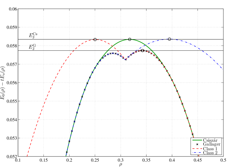
Figure 1: Error exponent bounds. Csiszár’s and Gallager’s curves correspond to $\bar{E}_{0}(\rho,W)-tE_{\text{s}}(\rho,P)$ and $E_{0}(\rho,W)-tE_{\text{s}}(\rho,P)$, respectively. Class $i$ curve correspond to $E_{0}(\rho,W)\;-\stackrel{{\scriptstyle[}}{{n\to\infty}}]{}{\lim}\frac{1}{n}E_{\text{s}}^{(i)}(\rho,P^{k})$, for $i=1,2$.

IV-C Example: a 6-input 4-output channel

We present an example in which the two-class partition (with their corresponding product distributions) attains the sphere-packing exponent while Gallager’s one-class assignment does not. Consider the source-channel pair composed by a binary memoryless source (BMS) and a non-symmetric memoryless channel with $|{\mathcal{X}}|=6$, $|{\mathcal{Y}}|=4$ and transition-probability matrix

$$W=\left(\begin{array}[]{c c c c}1-3\xi_{1}&\xi_{1}&\xi_{1}&\xi_{1}\\ \xi_{1}&1-3\xi_{1}&\xi_{1}&\xi_{1}\\ \xi_{1}&\xi_{1}&1-3\xi_{1}&\xi_{1}\\ \xi_{1}&\xi_{1}&\xi_{1}&1-3\xi_{1}\\ \frac{1}{2}-\xi_{2}&\frac{1}{2}-\xi_{2}&\xi_{2}&\xi_{2}\\ \xi_{2}&\xi_{2}&\frac{1}{2}-\xi_{2}&\frac{1}{2}-\xi_{2}\\ \end{array}\right).$$ (30)

This channel is similar to the channel given in [3, Fig. 5.6.5] and studied in [2] for source-channel coding. It is composed of two quaternary-output sub-channels: one of them is a quaternary-input symmetric channel with parameter $\xi_{1}$, and the second one is a binary-input channel with parameter $\xi_{2}$. We set $\xi_{1}=0.065$, $\xi_{2}=0.01$, $t=2$ and $P(1)=0.028$. It follows that the source entropy is $H(V)=0.1843$ bits/source symbol, the channel capacity is $C=0.9791$ bits/channel use and the critical rate is $R_{\text{cr}}=0.4564$ bits/channel use. Let $R^{\star}$ denote the value of $R$ minimizing (15). In this example we have $R^{\star}=0.6827>R_{\text{cr}}$ and $E_{\text{J}}^{\text{Cs}}$ is tight.

In Fig. 1 we plot the objective functions of Gallager’s exponent in (14) and Csiszár’s exponent in (16) as functions of $\rho$, respectively. For reference purposes, we also show the values of $E_{\text{J}}^{\text{G}}$ and $E_{\text{J}}^{\text{Cs}}$ with horizontal solid lines. The distribution $Q$ maximizing $E_{0}(\rho,W,Q)$ changes from $\bigl{(}\frac{1}{4}\;\frac{1}{4}\;\frac{1}{4}\;\frac{1}{4}\;0\;0\bigr{)}$ for $\rho\leq 0.31$ to $\bigl{(}0\;0\;0\;0\;\frac{1}{2}\;\frac{1}{2}\bigr{)}$ for $\rho>0.31$. As a result, $E_{0}(\rho,W)$ is not concave in $\rho\in[0,1]$. The figure shows how the non-concavity of Gallager’s function around the optimal $\rho$ of Csiszár’s function translates into a loss in exponent.

Fig. 1 also shows the bracketed terms in the RHS of (18) as a function of $\rho_{i}$ for the two-class partition of Theorem 2. The overall error exponent of the two-class construction is obtained by first individually maximizing the exponent of each of the curves over $\rho_{i}$, and by then choosing the minimum of the two individual maxima. In this example, the exponent of both classes coincides with $E_{\text{J}}^{\text{Cs}}$. The overall exponent is thus given by $E_{\text{J}}^{\text{Cs}}$, which is in agreement with Theorem 2.

V Conclusions

We have studied the error probability of random-coding ensembles where different codeword distributions are assigned to different subsets of source messages. We have showed that the random-coding exponent of ensembles generated with a single distribution does not attain Csiszár’s exponent in general. In contrast, ensembles with at most two appropriately chosen subsets and distributions suffice to attain the sphere-packing exponent in those cases where it is tight. One of the strengths of our achievability result is that, unlike Csiszár’s approach, it does not rely on the method of types. This leads to tighter bounds on the average error probability for finite block lengths and may simplify the task of generalizing our bound to source-channel systems with non-discrete alphabets and memory.

Appendix A Proof of Theorem 1

Generalizing the proof of the random-coding union bound for channel coding [12, Th. 16] (with earlier precedents in [3, pp. 136-137]) to the cases where codewords are independently generated according to distributions that depend on the class index of the source, we obtain

$$\epsilon \leq \sum_{i=1}^{N_{k}}\sum_{{\boldsymbol{v}}\in{\mathcal{A}}_{k}^{(i)}}P^{k}({\boldsymbol{v}})\sum_{{\boldsymbol{x}},{\boldsymbol{y}}}Q^{n}_{i}({\boldsymbol{x}})W^{n}({\boldsymbol{y}}|{\boldsymbol{x}})\min\left\{1,\sum_{j=1}^{N_{k}}\sum_{\bar{{\boldsymbol{v}}}\in{\mathcal{A}}_{k}^{(j)}}\sum_{\begin{subarray}{c}\bar{{\boldsymbol{x}}}:P^{k}(\bar{{\boldsymbol{v}}})W^{n}({\boldsymbol{y}}|\bar{{\boldsymbol{x}}})\\ \geq P^{k}({\boldsymbol{v}})W^{n}({\boldsymbol{y}}|{\boldsymbol{x}})\end{subarray}}Q^{n}_{j}(\bar{{\boldsymbol{x}}})\right\}.$$ (31)

We next use Markov’s inequality for $s_{j}\geq 0$, $j=1,\ldots,N_{k}$, to obtain [3]

$$\sum_{\begin{subarray}{c}\bar{{\boldsymbol{x}}}:P^{k}(\bar{{\boldsymbol{v}}})W^{n}({\boldsymbol{y}}|\bar{{\boldsymbol{x}}})\\ \geq P^{k}({\boldsymbol{v}})W^{n}({\boldsymbol{y}}|{\boldsymbol{x}})\end{subarray}}Q^{n}_{j}(\bar{{\boldsymbol{x}}})\leq\sum_{\bar{{\boldsymbol{x}}}}Q^{n}_{j}(\bar{{\boldsymbol{x}}})\Biggl{(}\frac{P^{k}(\bar{{\boldsymbol{v}}})W^{n}({\boldsymbol{y}}|\bar{{\boldsymbol{x}}})}{P^{k}({\boldsymbol{v}})W^{n}({\boldsymbol{y}}|{\boldsymbol{x}})}\Biggr{)}^{s_{j}}.$$ (32)

Using (32) and the inequality $\min\{1,A+B\}\leq A^{\rho}+B^{\rho^{\prime}}$, $A,B\geq 0$, $\rho,\rho^{\prime}\in[0,1]$ [3], (31) is upper-bounded by

$${\epsilon} \leq \sum_{i,j=1}^{N_{k}}\sum_{{\boldsymbol{v}}\in{\mathcal{A}}_{k}^{(i)}}P^{k}({\boldsymbol{v}})\sum_{{\boldsymbol{x}},{\boldsymbol{y}}}Q^{n}_{i}({\boldsymbol{x}})W^{n}({\boldsymbol{y}}|{\boldsymbol{x}})$$ (33)

$$\qquad\qquad{}\times\left(\sum_{\bar{{\boldsymbol{v}}}\in{\mathcal{A}}_{k}^{(j)}}\sum_{\bar{{\boldsymbol{x}}}}Q^{n}_{j}(\bar{{\boldsymbol{x}}})\Biggl{(}\frac{P^{k}(\bar{{\boldsymbol{v}}})W^{n}({\boldsymbol{y}}|\bar{{\boldsymbol{x}}})}{P^{k}({\boldsymbol{v}})W^{n}({\boldsymbol{y}}|{\boldsymbol{x}})}\Biggr{)}^{s_{j}}\right)^{\rho_{ij}},$$

where $\rho_{ij}\in[0,1]$ and $s_{j}\geq 0$, $i,j=1,\ldots,N_{k}$.

For $s_{i},s_{j}\in\bigl{[}\frac{1}{2},1\bigr{]}$ and $\rho_{ij}=\frac{1-s_{i}}{s_{j}}$, (33) yields

$$\epsilon \leq \sum_{i,j=1}^{N_{k}}\sum_{{\boldsymbol{y}}}G_{i}({\boldsymbol{y}})^{s_{i}}G_{j}({\boldsymbol{y}})^{1-s_{i}}$$ (34)

where

$$G_{i}({\boldsymbol{y}}) \triangleq \left(\sum_{{\boldsymbol{v}}\in{\mathcal{A}}_{k}^{(i)}}P^{k}({\boldsymbol{v}})^{s_{i}}\right)^{\frac{1}{s_{i}}}\Biggr{(}\sum_{{\boldsymbol{x}}}Q^{n}_{i}({\boldsymbol{x}})W^{n}({\boldsymbol{y}}|{\boldsymbol{x}})^{s_{i}}\Biggr{)}^{\frac{1}{s_{i}}}.$$ (35)

This choice of $\rho_{ij}$ allows us to decompose the probability of the “inter-class” error event between classes $i$ and $j$ as the product of two terms corresponding to the “intra-class” error events of each class. The RHS of (35) is further upper-bounded by

$$\epsilon \leq \sum_{i,j=1}^{N_{k}}\left(\sum_{{\boldsymbol{y}}}G_{i}({\boldsymbol{y}})\right)^{s_{i}}\left(\sum_{{\boldsymbol{y}}}G_{j}({\boldsymbol{y}})\right)^{1-s_{i}}$$ (36)

$$\leq \sum_{i,j=1}^{N_{k}}\left(s_{i}\left(\sum_{{\boldsymbol{y}}}G_{i}({\boldsymbol{y}})\right)+(1-s_{i})\left(\sum_{{\boldsymbol{y}}}G_{j}({\boldsymbol{y}})\right)\right)$$ (37)

$$\leq \sum_{i=1}^{N_{k}}\sum_{{\boldsymbol{y}}}G_{i}({\boldsymbol{y}})+\sum_{\begin{subarray}{c}i,j=1\\ i\neq j\end{subarray}}^{N_{k}}\left(\sum_{{\boldsymbol{y}}}G_{i}({\boldsymbol{y}})+\frac{1}{2}\sum_{{\boldsymbol{y}}}G_{j}({\boldsymbol{y}})\right)$$ (38)

$$= \frac{3N_{k}-1}{2}\sum_{i=1}^{N_{k}}\sum_{{\boldsymbol{y}}}G_{i}({\boldsymbol{y}}),$$ (39)

where in (36) we applied Hölder’s inequality $\|fg\|\leq\|f\|_{p}\|g\|_{q}$ with $p=\frac{1}{s_{i}}$ and $q=\frac{1}{1-s_{i}}$; (37) follows from the relation between arithmetic and geometric means; and (38) follows because $\frac{1}{2}\leq s_{i}\leq 1$. By identifying

$$\sum_{{\boldsymbol{y}}}G_{i}({\boldsymbol{y}})=\exp\Biggl{(}-E_{0}\left(\frac{1-s_{i}}{s_{i}},W^{n},Q^{n}_{i}\right)+E_{\text{s}}^{(i)}\left(\frac{1-s_{i}}{s_{i}},P^{k}\right)\Biggr{)}$$ (40)

and optimizing over $\frac{1}{2}\leq s_{i}\leq 1$, $i=1,\ldots,N_{k}$, it follows that

$$\epsilon\leq\frac{3N_{k}-1}{2}\sum_{i=1}^{N_{k}}\exp\biggl{(}-\max_{\rho_{i}\in[0,1]}\Bigl{\{}E_{0}\bigl{(}\rho_{i},W^{n},Q^{n}_{i}\bigr{)}-E_{\text{s}}^{(i)}(\rho_{i},P^{k})\Bigr{\}}\biggr{)},$$ (41)

where we denote $\frac{1-s_{i}}{s_{i}}$ by $\rho_{i}$. This concludes the proof.

Appendix B Proof of Theorem 2

The proof of the Theorem 2 is based on the next preliminary result.

Lemma 1

For any $\rho_{0}\in[0,1]$ and $\gamma^{\prime}\geq 0$, the partition (21)-(22) with $\gamma=\min\{1,\gamma^{\prime}\}$ satisfies

$$\frac{1}{k}E_{\text{s}}^{(1)}(\rho,P^{k}) \leq E_{\text{s}}(\rho,P)\leavevmode\hbox{\small 1\normalsize\kern-3.30002pt1}\{\rho>\rho_{0}\}+r(\rho,\rho_{0},\gamma^{\prime})\leavevmode\hbox{\small 1\normalsize\kern-3.30002pt1}\{\rho\leq\rho_{0}\}\triangleq\bar{E}_{\text{s}}^{(1)}(\rho,\rho_{0},\gamma^{\prime}),$$ (42)

$$\frac{1}{k}E_{\text{s}}^{(2)}(\rho,P^{k}) \leq E_{\text{s}}(\rho,P)\leavevmode\hbox{\small 1\normalsize\kern-3.30002pt1}\{\rho<\rho_{0}\}+r(\rho,\rho_{0},\gamma^{\prime})\leavevmode\hbox{\small 1\normalsize\kern-3.30002pt1}\{\rho\geq\rho_{0}\}\triangleq\bar{E}_{\text{s}}^{(2)}(\rho,\rho_{0},\gamma^{\prime}),$$ (43)

where $\leavevmode\hbox{\small 1\normalsize\kern-3.30002pt1}\{\cdot\}$ denotes the indicator function, and where

$$r(\rho,\rho_{0},\gamma)\triangleq E_{\text{s}}(\rho_{0},P)+\frac{E_{\text{s}}(\rho_{0},P)-\log\gamma}{1+\rho_{0}}\left(\rho-\rho_{0}\right).$$ (44)

Proof:

For the choice $\gamma=\min\{1,\gamma^{\prime}\}$ it holds that

$$\leavevmode\hbox{\small 1\normalsize\kern-3.30002pt1}\left\{P^{k}({\boldsymbol{v}})<\gamma^{k}\right\}\leq\leavevmode\hbox{\small 1\normalsize\kern-3.30002pt1}\left\{P^{k}({\boldsymbol{v}})\leq\gamma^{k}\right\}=\leavevmode\hbox{\small 1\normalsize\kern-3.30002pt1}\left\{P^{k}({\boldsymbol{v}})\leq(\gamma^{\prime})^{k}\right\}$$ (45)

since $P^{k}({\boldsymbol{v}})\leq 1$ for all ${\boldsymbol{v}}$. Using (45) and the bound $\leavevmode\hbox{\small 1\normalsize\kern-3.30002pt1}\{a\leq b\}\leq a^{-s}b^{s}$ for $s\geq 0$, the function $\frac{1}{k}E_{\text{s}}^{(1)}(\rho,P^{k})$ can be upper-bounded as

$$\frac{1}{k}E_{\text{s}}^{(1)}(\rho,P^{k}) \leq\frac{1}{k}\log\left(\sum_{{\boldsymbol{v}}}P^{k}({\boldsymbol{v}})^{\frac{1}{1+\rho}}\leavevmode\hbox{\small 1\normalsize\kern-3.30002pt1}\left\{P^{k}({\boldsymbol{v}})\leq(\gamma^{\prime})^{k}\right\}\right)^{1+\rho}$$ (46)

$$\leq\frac{1}{k}\log\left(\sum_{{\boldsymbol{v}}}P^{k}({\boldsymbol{v}})^{\frac{1}{1+\rho}}P^{k}({\boldsymbol{v}})^{-s}(\gamma^{\prime})^{ks}\right)^{1+\rho}$$ (47)

$$=\log\left(\sum_{v}P(v)^{\frac{1}{1+\rho}-s}(\gamma^{\prime})^{s}\right)^{1+\rho},$$ (48)

for any $s\geq 0$. Here we used that $P^{k}({\boldsymbol{v}})$ is memoryless. We continue by choosing $s$ such that

$$s =\max\left(0,\frac{\rho_{0}-\rho}{(1+\rho_{0})(1+\rho)}\right).$$ (49)

For $\rho>\rho_{0}$, it then follows that $s=0$, and (48) gives (cf. (5))

$$\frac{1}{k}E_{\text{s}}^{(1)}(\rho,P^{k}) \leq E_{\text{s}}(\rho,P).$$ (50)

For $\rho\leq\rho_{0}$, the choice (49) yields $s=\frac{\rho_{0}-\rho}{(1+\rho_{0})(1+\rho)}$, which together with (48) yields

$$\frac{1}{k}E_{\text{s}}^{(1)}(\rho,P^{k}) \leq(1+\rho)\log\left(\sum_{v}P(v)^{\frac{1}{1+\rho_{0}}}\right)-\frac{\rho-\rho_{0}}{1+\rho_{0}}\log\gamma^{\prime}$$ (51)

$$=(1+\rho_{0})\log\left(\sum_{v}P(v)^{\frac{1}{1+\rho_{0}}}\right)+(\rho-\rho_{0})\log\left(\sum_{v}P(v)^{\frac{1}{1+\rho_{0}}}\right)-\frac{\rho-\rho_{0}}{1+\rho_{0}}\log\gamma^{\prime}$$ (52)

$$=E_{\text{s}}(\rho_{0},P)+\frac{E_{\text{s}}(\rho_{0},P)-\log\gamma^{\prime}}{1+\rho_{0}}\left(\rho-\rho_{0}\right),$$ (53)

where in (52) we added and subtracted the term $\rho_{0}\log\left(\sum_{v}P(v)^{\frac{1}{1+\rho_{0}}}\right)$; and (53) follows from the definition (5). The inequality (42) follows by combining (50) and (51)-(53) for $\rho>\rho_{0}$ and $\rho\leq\rho_{0}$, respectively.

In an analogous way, the inequality (43) can be proved using that $\leavevmode\hbox{\small 1\normalsize\kern-3.30002pt1}\{P^{k}({\boldsymbol{v}})\geq\gamma^{k}\}=\leavevmode\hbox{\small 1\normalsize\kern-3.30002pt1}\{P^{k}({\boldsymbol{v}})\geq(\gamma^{\prime})^{k}\}$ and $\leavevmode\hbox{\small 1\normalsize\kern-3.30002pt1}\{a\geq b\}\leq a^{s}b^{-s}$ with $s\geq 0$. ∎

By applying Theorem 1 to the two-class partition (21)-(22) with associated product distributions $Q^{n}_{i}$, $i=1,2$, for the optimal threshold $\gamma$ we obtain

$$E_{\text{J}}^{\text{B}} \triangleq\max_{\gamma\in[0,1]}\left\{\liminf_{n\to\infty}\left\{-\frac{1}{n}\log\Biggl{(}h(k)\sum_{i=1,2}e^{-\stackrel{{\scriptstyle[}}{{\rho_{i}\in[0,1]}}]{}{\max}\bigl{\{}nE_{0}(\rho_{i},W,Q_{i})-E_{\text{s}}^{(i)}(\rho_{i})\bigr{\}}}\Biggr{)}\right\}\right\}$$ (54)

$$=\max_{\gamma\in[0,1]}\left\{\liminf_{n\to\infty}\min_{i=1,2}\left\{\max_{\rho_{i}\in[0,1]}\left\{E_{0}(\rho_{i},W,Q_{i})-\frac{1}{n}E_{\text{s}}^{(i)}(\rho_{i})\right\}\right\}\right\}$$ (55)

$$\geq\max_{\gamma^{\prime}\geq 0}\max_{\rho_{0},\rho_{1},\rho_{2}\in[0,1]}\min_{i=1,2}\left\{E_{0}(\rho_{i},W,Q_{i})-t\bar{E}_{\text{s}}^{(i)}(\rho_{i},\rho_{0},\gamma^{\prime})\right\}$$ (56)

$$\geq\max_{\begin{subarray}{c}\rho_{0},\rho_{1},\rho_{2}\in[0,1]:\\ \rho_{1}\leq\rho_{0}\leq\rho_{2}\end{subarray}}\max_{\gamma^{\prime}\geq 0}\min_{i=1,2}\left\{E_{0}(\rho_{i},W,Q_{i})-t\bar{E}_{\text{s}}^{(i)}(\rho_{i},\rho_{0},\gamma^{\prime})\right\},$$ (57)

where (55) follows by noting that $h(k)$ is subexponential in $k$; in (56) we have applied Lemma 1 with $\rho_{0}\in[0,1]$ and $\gamma^{\prime}\geq 0$ and have used that $\liminf_{n\to\infty}\max_{x}\{f_{n}(x)\}\geq\max_{x}\left\{\lim_{n\to\infty}f_{n}(x)\right\}$ as long as $\lim_{n\to\infty}f_{n}(x)$ exists for every $x$; and in (57) we have restricted the range over which we maximize $\rho_{i}$, $i=0,1,2$ and interchanged the maximization order.

By substituting (42)-(43) with $0\leq\rho_{1}\leq\rho_{0}\leq\rho_{2}\leq 1$, the minimization in (57) becomes

$$\min_{i=1,2}\left\{E_{0}(\rho_{i},W,Q_{i})+t\frac{E_{\text{s}}(\rho_{0},P)-\log\gamma^{\prime}}{1+\rho_{0}}(\rho_{0}-\rho_{i})-tE_{\text{s}}(\rho_{0},P)\right\}.$$ (58)

We define $\gamma_{0}\geq 0$ as the value satisfying

$$t\frac{E_{\text{s}}(\rho_{0},P)-\log\gamma_{0}}{1+\rho_{0}}=\frac{E_{0}(\rho_{2},W,Q_{2})-E_{0}(\rho_{1},W,Q_{1})}{\rho_{2}-\rho_{1}}.$$ (59)

The existence of such $\gamma_{0}$ follows from the continuity of the logarithm function. Choosing $\gamma^{\prime}=\gamma_{0}$ equalizes the two terms in the minimization in (58), thus maximizing the lower bound (57). As a result, substituting (58) into (57) we obtain

$$E_{\text{J}}^{\text{B}} \geq\max_{\rho_{0}\in[0,1]}\left\{\max_{\begin{subarray}{c}\rho_{1},\rho_{2}\in[0,1]:\\ \rho_{1}\leq\rho_{0}\leq\rho_{2}\end{subarray}}\left\{\frac{\rho_{2}-\rho_{0}}{\rho_{2}-\rho_{1}}E_{0}(\rho_{1},W,Q_{1})+\frac{\rho_{0}-\rho_{1}}{\rho_{2}-\rho_{1}}E_{0}(\rho_{2},W,Q_{2})\right\}-tE_{\text{s}}(\rho_{0},P)\right\}.$$ (60)

We now optimize the RHS of (60) over the assignments $(Q_{1},Q_{2})=(Q,Q^{\prime})$ and $(Q_{1},Q_{2})=(Q^{\prime},Q)$. By denoting by $\rho$ (resp. $\rho^{\prime}$) the variable $\rho_{i}$, $i=1,2$, associated to $Q$ (resp. $Q^{\prime}$) and defining $\lambda$ such that $\lambda\rho+(1-\lambda)\rho^{\prime}=\rho_{0}$, the optimal assignment leads to

$$E_{\text{J}}^{\text{B}} \geq\max_{\rho_{0}\in[0,1]}\left\{\max_{\begin{subarray}{c}\rho,\rho^{\prime},\lambda\in[0,1]:\\ \lambda\rho+(1-\lambda)\rho^{\prime}=\rho_{0}\end{subarray}}\Bigl{\{}\lambda E_{0}(\rho,W,Q)+(1-\lambda)E_{0}(\rho^{\prime},W,Q^{\prime})\Bigr{\}}-tE_{\text{s}}(\rho_{0},P)\right\}.$$ (61)

Theorem 2 follows from (61) by noting that [4, Th. 5.6]

$$\bar{E}_{0}(\rho_{0},W,\{Q,Q^{\prime}\})=\max_{\begin{subarray}{c}\rho,\rho^{\prime},\lambda\in[0,1]:\\ \lambda\rho+(1-\lambda)\rho^{\prime}=\rho_{0}\end{subarray}}\Bigl{\{}\lambda E_{0}(\rho,W,Q)+(1-\lambda)E_{0}(\rho^{\prime},W,Q^{\prime})\Bigr{\}}.$$ (62)

A two-class partition achieving the bound in Theorem 2 is given by (21)-(22), with $\gamma=\min(1,\gamma_{0}^{\star})$ where $\gamma_{0}^{\star}$ is computed from (59) for the values of $\rho_{0}^{\star}$, $\rho_{1}^{\star}$, $\rho_{2}^{\star}$ optimizing (60) and the assignment $(Q_{1}^{\star},Q_{2}^{\star})$ which leads to (61).

Appendix C Proof of Theorem 3

Before proving the result, we give some definitions that ease the exposition. Let ${\mathcal{A}}$ be an arbitrary non-empty discrete set. We denote the set of all probability distributions on ${\mathcal{A}}$ by ${\mathcal{D}}({\mathcal{A}})$ and the set of types in ${\mathcal{A}}^{n}$ by $\mathcal{D}_{n}({\mathcal{A}})$. We further denote by ${\mathcal{T}}({\sf P}_{XY})$ the type-class of sequences $({\boldsymbol{x}},{\boldsymbol{y}})$ with joint type ${\sf P}_{XY}$. The set ${\mathcal{L}}_{n}(P_{XY})$ is given by

$${\mathcal{L}}_{n}(P_{XY})\triangleq\Bigl{\{}\bar{{\sf P}}_{XY}\in{\mathcal{D}}_{n}(\mathcal{X}\times\mathcal{Y}):\bar{{\sf P}}_{Y}=P_{Y},\mathbb{E}\bigl{[}\log W(\bar{Y}|\bar{X})\bigr{]}\geq\mathbb{E}\bigl{[}\log W(Y|X)\bigr{]}\Bigr{\}},$$ (63)

where $(\bar{X},\bar{Y})\sim\bar{{\sf P}}_{XY}$ and $(X,Y)\sim P_{XY}$, and $P_{Y}$ denotes the marginal distribution of $P_{XY}$. Here, and throughout this appendix, we indicate that ${\boldsymbol{A}}$ is distributed according to the distribution $P_{{\boldsymbol{A}}}$ by writing ${\boldsymbol{A}}\sim P_{{\boldsymbol{A}}}$. Analogously, we define the set ${\mathcal{L}}(P_{XY})$ as

$${\mathcal{L}}(P_{XY}) \triangleq\Bigl{\{}\bar{P}_{XY}\in{\mathcal{D}}(\mathcal{X}\times\mathcal{Y}):\bar{P}_{Y}=P_{Y},\mathbb{E}\bigl{[}\log W(\bar{Y}|\bar{X})\bigr{]}\geq\mathbb{E}\bigl{[}\log W(Y|X)\bigr{]}\Bigr{\}},$$ (64)

with $(\bar{X},\bar{Y})\sim\bar{P}_{XY}$ and $(X,Y)\sim P_{XY}$.

Extending [13, Th. 1] to source-channel coding, we find that

$$\bar{\epsilon}\geq\frac{1}{4}\sum_{i=1}^{N^{\prime}_{k}}\sum_{{\boldsymbol{v}}\in{\mathcal{T}}_{i}}P({\boldsymbol{v}})\mathbb{E}\Biggl{[}\min\biggl{\{}1,\sum_{\bar{{\boldsymbol{v}}}\in{\mathcal{T}}_{i}}\Pr\Bigl{\{}{P^{k}(\bar{{\boldsymbol{v}}})W^{n}({\boldsymbol{Y}}|\bar{{\boldsymbol{X}}}_{i})\geq P^{k}({\boldsymbol{v}})W^{n}({\boldsymbol{Y}}|{\boldsymbol{X}}_{i})}\bigl{|}{\boldsymbol{X}}_{i}{\boldsymbol{Y}}\Bigr{\}}\biggr{\}}\Biggr{]},$$ (65)

where $({\boldsymbol{X}}_{i},{\boldsymbol{Y}})\sim Q^{n}_{i}\times W^{n}$ and $\bar{{\boldsymbol{X}}}_{i}\sim Q^{n}_{i}$. Here we have lower-bounded $\bar{\epsilon}$ by only considering in the inner sum those $\bar{{\boldsymbol{v}}}$ that are in the source type class ${\mathcal{T}}_{i}$, $i=1,\dotsc,N^{\prime}_{k}$.

We rewrite this bound in terms of summations over types with

$$\bar{\epsilon} \geq\frac{1}{4}\sum_{i=1}^{N^{\prime}_{k}}\sum_{{\sf P}_{XY}}\Pr\left\{{\boldsymbol{V}}\in{\mathcal{T}}_{i}\right\}\Pr\bigl{\{}({\boldsymbol{X}}_{i},{\boldsymbol{Y}})\in{\mathcal{T}}({\sf P}_{XY})\bigr{\}}$$

$$\qquad\qquad\times\min\left\{1,\sum_{\bar{{\sf P}}_{XY}\in{\mathcal{L}}_{n}({\sf P}_{XY})}\bigl{|}{\mathcal{T}}_{i}\bigr{|}\Pr\Bigl{\{}(\bar{{\boldsymbol{X}}}_{i},{\boldsymbol{y}})\in{\mathcal{T}}(\bar{{\sf P}}_{XY})\;\big{|}\;{\boldsymbol{y}}\in\bar{{\sf P}}_{Y}\Bigr{\}}\right\},$$ (66)

where ${\boldsymbol{V}}\sim P^{k}$.

Applying [14, Lemma 2.3] and [14, Lemma 2.6], we obtain

$$\bar{\epsilon} \geq\sum_{i=1}^{N^{\prime}_{k}}\sum_{{\sf P}_{XY}}\exp\Bigl{(}-kD({\sf P}_{i}\|P)-nD({\sf P}_{XY}\|Q_{i}\times W)+\delta^{\prime}_{k,n}-\log 4\Bigr{)}$$

$$\qquad\qquad\times\min\left\{1,\sum_{\bar{{\sf P}}_{XY}\in{\mathcal{L}}_{n}({\sf P}_{XY})}\exp\Bigl{(}kH(V_{i})-nD(\bar{{\sf P}}_{XY}\|Q_{i}\times\bar{{\sf P}}_{Y})+\delta^{\prime}_{k,n}\Bigr{)}\right\},$$ (67)

where $V_{i}\sim{\sf P}_{i}$ and $\delta^{\prime}_{k,n}\triangleq\log(k+1)^{-|\mathcal{V}|}(n+1)^{-|\mathcal{X}||\mathcal{Y}|}$.

The error probability can be further bounded by keeping only the leading exponential term in each summation in (67). Taking logarithms on both sides of (67), multiplying the result by $-\frac{1}{n}$, and using the notation $[x]^{+}=\max(x,0)$ we obtain

$$-\frac{\log\bar{\epsilon}}{n} \leq\min_{i=1,\dotsc,N^{\prime}_{k}}\min_{{\sf P}_{XY}}\min_{\bar{{\sf P}}_{XY}\in{\mathcal{L}}_{n}({\sf P}_{XY})}\Biggl{\{}\frac{k}{n}D({\sf P}_{i}\|P)+D({\sf P}_{XY}\|Q_{i}\times W)$$

$$\qquad\qquad\qquad\qquad\qquad\qquad\;\;\;\;+\left[D(\bar{{\sf P}}_{XY}\|Q_{i}\times\bar{{\sf P}}_{Y})-\frac{k}{n}H(V_{i})\right]^{+}\Biggr{\}}-\frac{\delta_{k,n}}{n},$$ (68)

where we define $\delta_{k,n}\triangleq 2\delta_{k,n}^{\prime}+\log 4$. Here we use that $[nx]^{+}=n[x]^{+}$, for $n>0$, that $[x]^{+}=\max(0,x)$ is monotonically non-decreasing, and that $[x+a]^{+}\leq[x]^{+}+a$, $a>0$.

Any distribution in ${\mathcal{D}}({\mathcal{A}})$ can be written as the limit of a sequence of types in ${\mathcal{D}}_{n}({\mathcal{A}})$ [6, Sec. IV]. Hence, the uniform continuity of $D(A\|B)$ over the pair $(A,B)$ ensures that for every $P_{XY}$, and every $\xi_{1}>0$, there exists a sufficiently large $n$ such that

$$-\frac{\log\bar{\epsilon}}{n} \leq\min_{i=1,\dotsc,N^{\prime}_{k}}\min_{P_{XY}}\min_{\bar{P}_{XY}\in{\mathcal{L}}(P_{XY})}\Biggl{\{}\frac{k}{n}D({\sf P}_{i}\|P)+D(P_{XY}\|Q_{i}\times W)$$

$$\qquad\qquad\qquad\qquad\qquad\qquad\quad+\left[D(\bar{P}_{XY}\|Q_{i}\times\bar{P}_{Y})-\frac{k}{n}H(V_{i})\right]^{+}\Biggr{\}}-\frac{\delta_{k,n}}{n}+\xi_{1},$$ (69)

where we have replaced ${\mathcal{L}}_{n}({\sf P}_{XY})$ by ${\mathcal{L}}(P_{XY})$, and used that $[x+a]^{+}\leq[x]^{+}+a$, $a>0$.

It follows from [13, Th. 4] that

$$\min_{P_{XY}}\min_{\bar{P}_{XY}\in{\mathcal{L}}(P_{XY})}\left\{D(P_{XY}\|Q\times W)+[D(\bar{P}_{XY}\|Q\times\bar{P}_{Y})-R]^{+}\right\}\\ =\max_{\rho\in[0,1]}\bigl{\{}E_{0}(\rho,W,Q)-\rho R\bigr{\}},$$ (70)

so (69) is equivalent to

$$-\frac{\log\bar{\epsilon}}{n} \leq\min_{i=1,\dotsc,N^{\prime}_{k}}\Biggl{\{}\frac{k}{n}D({\sf P}_{i}\|P)+\max_{\rho\in[0,1]}\left\{E_{0}(\rho,W,Q_{i})-\rho\frac{k}{n}H(V_{i})\right\}\Biggr{\}}-\frac{\delta_{k,n}}{n}+\xi_{1}.$$ (71)

Maximizing (71) over $Q_{i}\in\mathcal{Q}$ for each $i=1,\ldots,N^{\prime}_{k}$ yields

$$-\frac{\log\bar{\epsilon}}{n} \leq\min_{i=1,\dotsc,N^{\prime}_{k}}\Biggl{\{}\frac{k}{n}D({\sf P}_{i}\|P)+\max_{\rho\in[0,1]}\left\{E_{0}(\rho,W,{\mathcal{Q}})-\rho\frac{k}{n}H(V_{i})\right\}\Biggr{\}}-\frac{\delta_{k,n}}{n}+\xi_{1}.$$ (72)

By taking $n$ to be sufficiently large in the outer bracketed term of (72), we obtain for $\xi_{2}>0$ that

$$-\frac{\log\bar{\epsilon}}{n} \leq\min_{i=1,\dotsc,N^{\prime}_{k}}\Biggl{\{}tD({\sf P}_{i}\|P)+\max_{\rho\in[0,1]}\left\{E_{0}(\rho,W,{\mathcal{Q}})-\rho tH(V_{i})\right\}\Biggr{\}}-\frac{\delta_{k,n}}{n}+\xi_{1}+\xi_{2}.$$ (73)

Using now the uniform continuity of the RHS of (73) as a function of ${\sf P}_{i}$ [1, p. 323] and that any distribution in $\mathcal{D}(\mathcal{V})$ can be written as the limit of a sequence of source types in $k$, it follows that for every $\xi_{3}>0$ there exists a sufficiently large $n$ such that

$$-\frac{\log\bar{\epsilon}}{n}\leq \min_{P^{\prime}}\Biggl{\{}tD(P^{\prime}\|P)+\max_{\rho\in[0,1]}\left\{E_{0}(\rho,W,{\mathcal{Q}})-\rho tH(V^{\prime})\right\}\Biggr{\}}-\frac{\delta_{k,n}}{n}+\xi_{1}+\xi_{2}+\xi_{3},$$ (74)

where $V^{\prime}\sim P^{\prime}$ . By taking the limit superior in $n$, this becomes

$$\limsup_{n\to\infty}-\frac{\log\bar{\epsilon}}{n}\leq \min_{P^{\prime}}\Bigl{\{}tD(P^{\prime}\|P)+\max_{\rho\in[0,1]}\left\{E_{0}(\rho,W,{\mathcal{Q}})-\rho tH(V^{\prime})\right\}\Bigr{\}}+\xi_{1}+\xi_{2}+\xi_{3}$$ (75)

$$= \min_{0\leq R\leq t\log|{\mathcal{V}}|}\Bigl{\{}te\left(\frac{R}{t},P\right)+\max_{\rho\in[0,1]}\left\{E_{0}(\rho,W,{\mathcal{Q}})-\rho R\right\}\Bigr{\}}+\xi_{1}+\xi_{2}+\xi_{3}$$ (76)

$$= \max_{\rho\in[0,1]}\bigl{\{}\bar{E_{0}}(\rho,W,{\mathcal{Q}})-tE_{\text{s}}(\rho,P)\bigr{\}}+\xi_{1}+\xi_{2}+\xi_{3},$$ (77)

where (76) follows from the definition of the source reliability function [1, eq. (7)] with $R=tH(V^{\prime})$; and (77) can be proved by the same methods that relate (15) and (16). Finally, letting $\xi_{1}$, $\xi_{2}$ and $\xi_{3}$ tend to zero from above yields the desired result.

References

• [1] I. Csiszár, “Joint source-channel error exponent,” Probl. Contr. Inf. Theory, vol. 9, pp. 315–328, 1980.
• [2] Y. Zhong, F. Alajaji, and L. L. Campbell, “On the joint source-channel coding error exponent for discrete memoryless systems,” IEEE Trans. Inf. Theory, vol. 52, no. 4, pp. 1450–1468, April 2006.
• [3] R. G. Gallager, Information Theory and Reliable Communication.   New York: John Wiley & Sons, Inc., 1968.
• [4] R. T. Rockafellar, Convex Analysis, 2nd ed.   Princeton, US: Princeton University Press, 1972.
• [5] F. Jelinek, Probabilistic Information Theory.   New York: McGraw-Hill, 1968.
• [6] I. Csiszár, “The method of types,” IEEE Trans. Inf. Theory, vol. 44, no. 6, pp. 2505–2523, 1998.
• [7] Y. Zhong, F. Alajaji, and L. Campbell, “Joint source–channel coding error exponent for discrete communication systems with Markovian memory,” IEEE Trans. Inf. Theory, vol. 53, no. 12, pp. 4457–4472, Dec. 2007.
• [8] ——, “Joint source–channel coding excess distortion exponent for some memoryless continuous-alphabet systems,” IEEE Trans. Inf. Theory, vol. 55, no. 3, pp. 1296–1319, March 2009.
• [9] A. Tauste Campo, G. Vazquez-Vilar, A. Guillén i Fàbregas, T. Koch, and A. Martinez, “Achieving Csiszár’s exponent for joint source-channel coding with product distributions,” in 2012 IEEE Int. Symp. on Inf. Theory, Boston, USA, July 2012.
• [10] A. Tauste Campo, G. Vazquez-Vilar, A. Guillen i Fabregas, T. Koch, and A. Martinez, “Random coding bounds that attain the joint source-channel exponent,” in 46th Annual Conference on Information Sciences and Systems (CISS 2012), Princeton, USA, March 2012, invited.
• [11] I. Csiszár, “On the error exponent of source-channel transmission with a distortion threshold,” IEEE Trans. Inf. Theory, vol. IT-28, no. 6, pp. 823–828, Nov. 1982.
• [12] Y. Polyanskiy, H. V. Poor, and S. Verdú, “Channel coding rate in the finite blocklength regime,” IEEE Trans. Inf. Theory, vol. 56, no. 5, pp. 2307–2359, May 2010.
• [13] J. Scarlett, A. Martinez, and A. Guillén i Fàbregas, “Ensemble tight error exponent for mismatched decoders,” in Proc. 50th Allerton Conf. on Comms. and Control, Monticello, IL, Oct. 1-5 2012.
• [14] I. Csiszár and J. Körner, Information Theory: Coding Theorems for Discrete Memoryless Systems, 2nd ed.   Cambridge University Press, 2011.