Liquid crystal elastomers and phase transitions in rod networks

Abstract

In this article, we construct and analyze models of anisotropic crosslinked polymers employing tools from the theory of liquid crystal elastomers. The anisotropy of these systems stems from the presence of rigid-rod molecular units in the network. We study minimization of the energy for incompressible as well as compressible materials, combining methods of isotropic nonlinear elasticity with the theory of lyotropic liquid crystals. We apply our results to the study of phase transitions in networks of rigid rods, in order to model the behavior of actin filament systems found in the cytoskeleton.

1 Introduction

Cytoskeletal networks consist of rigid, rod-like actin protein units jointed by flexible crosslinks, presenting coupled orientational and deformation effects analogous to liquid crystal elastomers. The alignment properties of the rigid rods influence the mechanical response of the network to applied stress and deformation, affecting functionality of the systems [34], [23]. Parameters that characterize these networks include the aspect ratio of the rods and the average length of the crosslinks, with a large span of parameter values found across in-vivo networks. For instance, cytoskeletal networks of red blood cells have very large linkers and small rod aspect ratio [33], [22], whereas those of cells of the outer hair of the ear have very large aspect ratio and short linkers favoring well aligned nematic, in order to achieve an efficient sound propagation [25].

This article is motivated by the works on Montecarlo simulations of phase transitions in rigid rod fluids by Bates el al. [6] and the later application to actin networks by Dalhaimer et al. [13]. In these articles, the authors discuss experimentally observed alignment states and their phases transitions as well as predictions from numerical experiments. They report on a wide range of anisotropic regimes, including the uncross-linked fluid network, in the nematic as well as the isotropic state, and the crystal-glass states involving elastomer microstructure. A goal of our work is to obtain a continuum model matching predictions of the molecular simulations and available experiments.

A nematic fluid consists of interacting rod-like molecules that have the tendency to aling along preferred directions and the ability to flow under applied forces. Liquid crystal elastomers are anisotropic nonlinear elastic materials, with the source of anisotropy stemming from elongated, rigid monomer side groups, or from main chain rod-like elements. They are elastic solids that may also present fluid regimes of [12], ([14], [15], [20], [35]). The interaction between the rod units and the network is at the core of liquid crystal elastomer behavior. In main chain elastomers, the connected rigid units are part of the backbone chains of the system and in side-chain elastomers, the rod units are attached to the polymer backbone. In both cases, the backbone chains are crosslinked into a network. Models of anisotropic polymer melts and their non-Newtonian behavior have received significant attention ([18], [32], [36]).

Ordering in nematic fluids is affected by temperature in thermotropic liquid crystals and by rod concentration in lyotropic ones. At high temperature or low concentration, respectively, nematic fluids are found in the isotropic state, experiencing a transition to the nematic upon cooling the thermotropic liquid or increasing the rod concentration of the lyotropic [24]. In rod-like systems, such as actin fiber networks, the phase transition behavior is affected by the density of rods.

We consider anisotropic systems such that the total energy is the sum of the Landau-de Gennes liquid crystal energy of the nematic and an anisotropic elastic stored energy function. This energy involves two sources of anisotropy expressed by symmetric second order tensors, that associated with the rigid units, represented by the nematic order tensor $Q$, and that of the network described by the positive definite, step-length tensor $L$. The tensor $L$ encodes the shape of the network: it is spherical for isotropic polymers and spheroidal for uniaxial nematic elastomers, and has eigenvalues $l_{\|}$ and $l_{\perp}$ (double). The quantity $r:=\frac{l_{\|}}{l_{\perp}}-1$ measures the degree of anisotropy of the network, with positive values corresponding to prolate systems and negative ones to the oblate shapes. In the prolate geometry, the eigenvector $\boldsymbol{n}$ associated with $l_{\|}$ is the director of the theory, giving the average direction of alignment of the rods and also the direction of shape elongation of the network. It is natural to assume that $L$ and $Q$ share eigenvectors. In particular we assume that they are linearly related, so that for $L$ prescribed, we take $Q$ as its traceless version, that is $Q=L-\frac{1}{3}{\textrm{tr}}LI$ ([35], page 49). The free energy may also carry information on the anisotropy $L_{0}$ imprinted in the network at crosslinking the original polymer melt.

The Landau-de Gennes free energy density is the sum of scalar quadratic terms of $\nabla Q$ and the bulk scalar function $f(Q)$. In the de Gennes-Landau theory, $f$ is a polynomial function of the trace of powers of $Q$ and describes the phase transition between the isotropic and the nematic phases [24]. However, the polynomial growth is not physically realistic since it is expected that an infinite energy should be required to reach limiting alignment configurations [7], [17]. This turns out to be as well an essential element of our analysis. A cautionary note about notation: we will employ the common symbol $f$ to denote the bulk nematic energy density in the different cases that we address.

Denoting $F$ the deformation gradient, the elastic energy density proposed by Blandon, Terentjev and Warner is $|L^{-\frac{1}{2}}FL_{0}^{\frac{1}{2}}|^{2}$. It is the analog of the Neo-Hookean energy of isotropic elasticity, and also derived from Gaussian statistical mechanics. Taking into account the relevant role played by the tensor $G:={(L^{-1}FF^{T}L_{0})}^{\frac{1}{2}}$ in the trace form of the energy, and motivated by the theory of existence of minimizers of isotropic nonlinear elasticity ([4]), we consider polyconvex stored energy density functions $w(\boldsymbol{X})=\hat{w}(G(\boldsymbol{X}))$, $\boldsymbol{X}\in\Omega$. That is, functions $\hat{w}$ such that there exists a convex function $\Psi$ of the invariants $\{I_{i}\}_{i=1,2,3}$ of $GG^{T}$ satisfying $\hat{w}(G)=\Psi(I_{1},I_{2},I_{3})$. However, since $G$ is not a gradient, we must be able to recover the limiting deformation gradient $F^{*}$ from the minimizing sequences $\{G_{k}\}_{k\geq 1}$. For this, it is necessary that the minimizing sequences $\{L_{k}\}$ yield a nonsingular limit. This is achieved, by either appropriately regularizing the problem so that the range of the eigenvalues of $Q$ in the admissible set is strictly greater than $-\frac{1}{3}$, or by requiring the blow up of $f(Q)$ at the minimum eigenvalue limit, that is, $f(Q)\to\infty$ as $\det(Q+\frac{1}{3}I)\to 0$.

In the case of compressible networks, we further assume that expansion and compression are coupled with order, so that the bulk free energy is now $f(Q,\det F)$. Following the analogous assumptions of isotropic elasticity, we require that, for each symmetric traceless tensor $Q$, $f$ becomes unbounded as $\det F\to\{0,\infty\}$. We argue that the coupling between expansion and compression with nematic order is qualitatively analogous to that of lyotropic uniaxial nematic liquid crystals, as proposed by Kuzuu and Doi [26]. In this case, the bulk energy $f(s)$ is parametrized by the rod concentration of the nematic fluid. At low concentration, the isotropic minimum dominates, with nematic becoming the preferred phase as the concentration increases. In the application to rigid rod networks of section 4, two parameter rates emerge as very relevant: $\chi=\frac{L_{a}}{L_{x}}$, where $L_{a}$ denotes the typical length of a cylindrical rod, and $L_{x}$ that of a cross-linker filament, and the aspect ratio $A_{a}=\frac{L_{a}}{D_{a}}$ of the rod where $D_{a}$ denotes a typical diameter. We assume that $f$ depends on $s$ and the rigid rod density $\rho$, and it is also parametrized by the ratio $\chi$. Specifically, following the denominations of loose, semiloose and tight for networks with small through large values of $\chi$, we assume that $f$ evolves from a function with a single isotropic well for $\chi$ small (large linkers), to having a single nematic well for large $\chi$ (short linkers), presenting an intermediate double-well region. We also assume that the liquid energy scales according to the aspect ratio of the rods, resulting in larger nematic contribution with increasing aspect ratio. Proposition 4.1 summarizes the results on phase transitions under three-dimensional expansion. In subsection 4.2.1, we construct a bulk free energy density with the previously described properties and present results on numerical simulations of the phase transition behavior under plane extensions, plots of phase diagrams in the density-aspect ratio plane, and the graphs of the equilibrium order parameter $s$ with respect to the rod density. In particular, we find oblate equilibrium states for small values of the aspect ratio, corresponding to disk-like molecules.

In addition to the trace models of liquid crystal elastomer energy studied by Terentjev and Warner ([35] and references therein), generalizations of these earlier forms have been proposed and studied by several authors ([2] and [19]; [1], [9], [10] and [16]). In the first two references, the authors propose energies based on powers of the earlier trace form, including Ogden type energies, and study their extensions to account for semisoft elasticity. Articles by de Simone et al. also propose and study Ogden type energies. Furthermore, the analysis of equilibrium states presented in [1] applies to elastomer energy density functions that are not quasiconvex. (For instance, these are appropriate to model crystal-like phase transitions.) Their methods of proof combine the construction of lower quasiconvex envelops, the rigidity theorem [21] and tools from the theory of $\Gamma$-convergence. Our results apply to a more restrictive class of energy density functions, that is, polyconvex functions with respect to the anisotropic deformation tensor $G$. Our methods of proof use tools of isotropic nonlinear elasticity, and as such, are directly tailored to treating polyconvexity. Moreover, this approach readily applies to modeling the nonconvexity associated with nematic liquid order in networks and the corresponding phase transitions, although it does not cover the more general type of transitions linked to quasiconvexity.

This article is organized as follows. Section 2 is devoted to modeling, which includes incompressible and compressible liquid crystal elastomers as well as a rod-fluid model. Section 3 is devoted to the minimization of the energy in the different cases. Section 4 presents a study of density dependent liquid crystal phase transitions, with figures corresponding to the phase transition diagram and the order properties with respect to mechanical extension of the system. The conclusions are described in Section 5.

Some of the results of section 3 follow from the Ph.D thesis dissertation by Chong Luo [28].

2 The Landau-de Gennes liquid crystal elastomer

Equilibrium states of nematic liquid crystal elastomers are characterized by the gradient of deformation tensor $F$ together with the symmetric tensors $L$ and $Q$, describing the shape of the network and the nematic order, respectively.

We let the open and bounded domain $\Omega\subset{\mathbf{R}}^{3}$ denote the reference configuration of the elastomer. We denote $L_{0}$ and $Q_{0}$, the network anisotropy and the nematic order, respectively. in the reference configuration. For synthetic elastomers, these tensors model the cross-linking, in fiber networks, these quantities represent the anisotropy and order in a relevant state, for instance, the stress free state if one exists. We denote the deformation map of the polymer and its gradient as

$$\boldsymbol{\varphi}:\Omega\longrightarrow\ \bar{\Omega},\quad\boldsymbol{x}=\boldsymbol{\varphi}(\boldsymbol{X}),$$ (1)

$$F=\nabla\boldsymbol{\varphi},\quad\det F>0.$$

In order to understand the relationship among them and how they enter in the energy, we start with a brief survey of these tensors at the molecular level, the following the treatment in [35].

2.1 Statistical mechanics of anisotropic polymers

We now focus on the statistical treatment of single ideal chains. Let us consider a freely jointed chain composed of $N$ segments of length $a$, and let $\mathbf{R}$ denote the end-to-end vector of a chain. The chain follows a random walk with step length $a$. The average end-to-end distance is given by

$$<|\mathbf{R}|^{2}>=Na^{2}=al,\quad<R_{i}R_{j}>=\frac{1}{3}\delta_{ij}al,\,\,1\leq i,j\leq 3,$$ (2)

where $l=Na$ is the arc length of the chain, and $<\cdot>$ denotes the ensemble average. The probability of a given chain conformation to have an end-to-end vector $\mathbf{R}$ is the Gaussian distribution

$$p_{N}(\mathbf{R})=(\frac{3}{2\pi R_{0}^{2}})^{\frac{3}{2}}e^{-\frac{3|\mathbf{R}|^{2}}{2R_{0}^{2}}},$$ (3)

characterized by its variance $R_{0}$. Moreover, consistency with (2) implies that $R_{0}=al$. The partition function,

$$Z_{N}(\mathbf{R})=p_{N}(\mathbf{R})Z_{N}$$

gives the number of configurations with end-to-end vector $\mathbf{R}$, where $Z_{N}$ is the total number of chain configurations. So, the free energy of a single chain is

$$\mathcal{F}=-k_{B}T\ln Z_{n}(\mathbf{R})=k_{B}T(\frac{3|\mathbf{R}|^{2}}{2R_{0}^{2}})+C,$$ (4)

where $C$ is constant.

Another measure of the spatial extension of a single chain is the radius of gyration $R_{G}$. It is defined as the root mean square of the distance between each segment of the chain and the center of mass. In the case that the number of segments $N>>1$,

$$<R_{G}^{2}>\approx\frac{1}{6}Na^{2}=\frac{1}{6}aL=\frac{1}{6}R_{0}.$$

So, in the average, the shape of a polymer chain at equilibrium is spherical with radius $R_{G}$.

The average shape of a liquid crystal polymer is that of an ellipsoid, with step-length tensor $L$, so that the anisotropic analog of the average of end-to-end distance (2) is now

$$<R_{i}R_{j}>=\frac{1}{3}lL_{ij}.$$ (5)

Letting $l_{1},l_{2}$ and $l_{3}$ denote the ellipsoid semi-axes along directions $\boldsymbol{e}_{i}$, $i=1,2,3$, $|\boldsymbol{e}_{i}|=1$, $L$ admits the spectral representation

$$L=\Sigma_{i=1}^{3}l_{i}\boldsymbol{e}_{i}\otimes\boldsymbol{e}_{i}.$$ (6)

We take $l_{1}=l_{2}:=l_{\perp}$ to represent a uniaxial network giving the spheroidal representation for L, and denote $l_{\|}:=l_{3}$ and $\boldsymbol{n}:=\boldsymbol{e}_{3}$, so that

$$L=(l_{\|}-l_{\perp})\boldsymbol{n}\otimes\boldsymbol{n}+l_{\perp}I.$$ (7)

In the prolate symmetry corresponding to main chain polymers, $l_{\|}>l_{\perp}$ in which case the polymer backbone will stretch along the nematic director $\boldsymbol{n}$. (The reverse inequality holds in the case of side-chain oblate elastomers).

The Gaussian distribution of chain conformations generalized to the anisotropic case is

$$p_{N}(\mathbf{R})=[(\frac{3}{2\pi l})^{3}\frac{1}{\det L}]^{\frac{1}{2}}e^{-\frac{3}{2l}(\mathbf{R}\cdot L^{-1}\mathbf{R})}.$$ (8)

As in the isotropic case, the affinity property of chain conformations leads to the anisotropic version of the neo-Hookean energy in the form

$$\mathcal{W}_{\textrm{\tiny{BTW}}}=\mu(F\cdot L^{-1}F),$$ (9)

where $\mu$ denotes the shear modulus. An expression that includes the shape at crosslinking encoded in the initial step-length tensor $L_{0}$ is

$$\mathcal{W}_{\textrm{\tiny{BTW}}}=\mu{\textrm{tr}}(L_{0}F^{T}L^{-1}F).$$ (10)

In general, scalar functions of powers of the tensors $FL_{0}F^{T}$ and $F^{T}L^{-1}F$ are admissible.

Following the property of freely joined rods, we assume that $L$ and $Q$ have common eigenvectors and propose the constitutive relation

$$L=a_{0}(Q+\frac{1}{3}I),$$ (11)

where $a_{0}={\textrm{tr}}L$ is constant. The linear constitutive equation (11) is analogous to those proposed by Terentjev and Warner [35] and Eliot and Sellers [19] stating that, given a symmetric and traceless tensor $Q$ and a constant $\beta>0$, there is a one $\alpha$-parameter family of step-length tensors $L$ with ${\textrm{tr}}L=\beta$, and such that

$$L=\beta(\alpha Q+\frac{1}{3}I).$$ (12)

The form (11) corresponds to taking $\alpha=1$ and $\beta=a_{0}$ in (12).

In order to interpret this condition, and following the approach in [29], we appeal to the spectral representation

$$Q=\sum_{i=1}^{3}\lambda_{1}\boldsymbol{e}_{i}\otimes\boldsymbol{e}_{i},\quad\lambda_{1}+\lambda_{2}+\lambda_{3}=0.$$ (13)

The eigenvalues of $Q$ satisfy $-\frac{1}{3}\leq\lambda_{i}\leq\frac{2}{3}$, $i=1,2,3$. For a biaxial nematic, $Q$ admits the representation in terms of the order parameters $r$ and $s$,

$$Q=r(\boldsymbol{e}_{1}\otimes\boldsymbol{e}_{1}-\frac{1}{3}I)+s(\boldsymbol{e}_{2}\otimes\boldsymbol{e}_{2}-\frac{1}{3}I),$$ (14)

where

$$s=\lambda_{1}-\lambda_{3}=2\lambda_{1}+\lambda_{2},\quad r=\lambda_{2}-\lambda_{3}=\lambda_{1}+2\lambda_{2}.$$

The inequality constraints on $\lambda_{i}$ imply restrictions on $r$ and $s$. Specifically, admissible values of $(r,s)$ belong to the interior of the triangle $\mathcal{T}$ determined by the edges $\partial\mathcal{T}$: $r+s=1,r-2s=1$ and $s-2r=1$ (Figure 1). It is easy to check that $Q$ reaches its minimum eigenvalue $\lambda=-\frac{1}{3}$ on each edge of $\partial\mathcal{T}$. Hence,

$$\det L=0\Leftrightarrow\det(Q+\frac{1}{3}I)=0\Leftrightarrow(r,s)\in\partial\mathcal{T}.$$ (15)

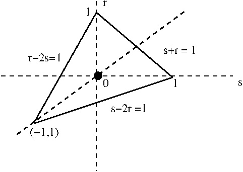
Fig. 1: $Q$ attains the minimum eigenvalue $\lambda=-\frac{1}{3}$ on each one of the edges of the triangle $\mathcal{T}$ [29].

We finally notice that the uniaxial states correspond to the lines $r=0,s=0$ and $r=s$. In the latter case, the uniaxial order tensor representation is

$$Q=-s(\boldsymbol{n}\otimes\boldsymbol{n}-\frac{1}{3}I),\,\,-s\in(-\frac{1}{2},1),\,|\boldsymbol{n}|=1,$$ (16)

with $\boldsymbol{n}:=\boldsymbol{e}_{3}$ representing the director of the theory. Consistency with (6) yields

$$a_{0}r=(l_{1}-l_{3}),\quad a_{0}s=(l_{2}-l_{3}).$$ (17)

This reduces to the uniaxial nematic with director $\boldsymbol{n}$ and order parameter $s$ in the case that

$$l_{2}=l_{1}:=l_{\perp},\,\,l_{3}:=l_{\|}.$$

We conclude this section introducing the following notation. Let ${\mathbb{M}}^{3}$ denote the space of three-dimensional tensors.

$$\mathbb{M}^{3}_{+}=\{M\in\mathbb{M}^{3}:\det M>0\},\quad\mathbb{S}^{3}=\{M\in\mathbb{M}^{3}:M=M^{T}\},$$ (18)

$$\mathbb{S}^{3}_{+}=\{M\in\mathcal{S}^{3}:\det M>0\},\quad\mathbb{S}^{3}_{0}=\{Q\in\mathbb{S}^{3}:\,\textrm{tr}\,Q=0\}.$$ (19)

The shape tensor $L\in\mathbb{S}^{3}_{+}$ and $Q\in\mathbb{S}^{3}_{0}$.

2.2 Energy functionals

We now present the energy expressions for liquid crystals and their coupling with the anisotropic elastic energy. This motivates the liquid crystal elastomer energies analyzed in this article.

2.2.1 Uniaxial liquid crystal energy

When using the uniaxial representation (16) on $Q$, the liquid crystal energy becomes that of the model of Ericksen for liquid crystals with variable degree of orientation,

$$\mathcal{W}_{\textrm{\tiny{E}}}=k(|\nabla s|^{2}+s^{2}|\nabla\boldsymbol{n}|^{2})+\nu f(s),$$ (20)

where $k>0$ denotes the nematic elastic constant. The bulk energy $f$ is assumed to be parametrized by the temperature, in thermotropic liquid crystals, and by the rod concentration, in lyotropic ones [17], [26] and [27]. High values of the rod concentration favor the nematic state, whereas dilute systems tend to be isotropic. This motivates us to consider nematic fluids with coupling of order and rod density $\rho$ by allowing the bulk energy density to depend on $\rho$ as well, that is, taking $f(\rho,s)$, as in the study of actin networks presented in section 4.

We point out that (20) follows from the Landau-de Gennes energy of biaxial nematics when setting the biaxial order parameter $r=0$ in (14).

2.2.2 Landau-de Gennes liquid crystal energy

In its original form, the Landau-de Gennes energy density is given by

$$\mathcal{W}_{\textrm{\tiny{LdG}}}=\nu f(Q)+k|\nabla Q|^{2}$$ (21)

where

$$f=a\,{\textrm{tr}}(Q^{2})-\frac{b}{3}{\textrm{tr}}(Q^{3})+\frac{c}{4}({\textrm{tr}}Q^{2})^{2},\quad a=\frac{\alpha}{2}(T-T_{NI}),$$ (22)

$a$, $b$, $c$ and $\alpha$ are positive, material dependent constants, $T$ denotes absolute temperature, and $T_{NI}$ is the temperature of transition between the isotropic and nematic phases. The parameterization of $f$ by $T$ has the effect of changing the relative depth of the potential wells, with the nematic minimum prevailing at low temperatures whereas the isotropic one has lowest energy at high temperature.

The polynomial form of the bulk energy $f(Q)$ poses physical and mathematical difficulties, so instead we assume that there exists a smooth function $\Phi:\mathcal{T}\to\boldsymbol{R}+$ such that

$$\,\,\,f(Q)=\Phi(s,r),$$ (23)

$$\lim_{(s.r)\to\partial\mathcal{T}}\Phi(s,r)=+\infty.$$ (24)

2.2.3 Incompressible liquid crystal elastomer

The total energy of a liquid crystal elastomer couples the anisotropic elastic free energy (10) with the Landau-de Gennes liquid crystal expression is given by

$$\mathcal{E}=\int_{\Omega}\frac{\mu}{2}\big{(}|L^{-\frac{1}{2}}FL_{0}^{\frac{1}{2}}|^{2}\big{)}+\nu f(Q)+k|\nabla Q|^{2}\,d\boldsymbol{X},$$ (25)

with $F$ satisfying $\det F=1$. For an incompressible uniaxial elastomer, it becomes

$$\mathcal{E}=\int_{\Omega}\big{(}\mathcal{W}_{\textrm{\tiny{BTW}}}(F,s,\boldsymbol{n},\boldsymbol{n}_{0})+\mathcal{W}_{\textrm{\tiny{E}}}(s,\boldsymbol{n})\big{)}\,d\boldsymbol{X},$$ (26)

with

$$\mathcal{W}_{\textrm{\tiny{BTW}}}= \frac{1}{2}\mu\frac{l_{\perp}^{0}}{l_{\perp}}\big{(}(|F|^{2}-(1-r)|F^{T}\boldsymbol{n}|^{2})$$

$$+ (\frac{1-r_{0}}{r_{0}})(|F\boldsymbol{n}_{0}|^{2}-(1-r)(F^{T}\boldsymbol{n}\cdot\boldsymbol{n}_{0})^{2})\big{)},$$

$$r= \frac{l_{\perp}}{l_{\|}},\,\,r_{0}=\frac{l_{\perp}^{0}}{l_{\|}^{0}},\quad\alpha:=1-r,$$ (27)

as in ([35]), with $\boldsymbol{n}_{0},l_{\|}^{0}$ and $l_{\perp}^{0}$ representing rod alignment and polymer shape, respectively, at crosslinking. From (27), we observe that the configuration at crosslinking is also the reference one.

2.2.4 Compressible liquid crystal elastomer

The energy of a compressible liquid crystal elastomer follows from (25) but now allowing deformations such that $\det F>0$, without the constraint of the determinant being equal to 1. Moreover, as in isotropic nonlinear elasticity, we assume that $f$ is also a function of $\det F$. That is,

$$\mathcal{E}=\int_{\Omega}\frac{\mu}{2}\big{(}|L^{-\frac{1}{2}}FL_{0}^{\frac{1}{2}}|^{2}\big{)}+\nu f(Q,\det F)+k|\nabla Q|^{2}\,d\boldsymbol{X},$$ (28)

where $\mu\geq 0,\nu\geq 0$ and $k\geq 0$ are prescribed material parameters. We point out that the function $f$ also encodes the isotropic to nematic phase transition behavior, and, in particular, it accounts for the observed change in volume in such a transition.

2.2.5 Nonlinear anisotropic elastic energy

We observe from the previous subsections that, due to the anisotropy, the energy of the liquid crystal elastomer depends on the deformation gradient $F$ through the combination

$$G:=L^{-\frac{1}{2}}FL_{0}^{\frac{1}{2}}=(L^{-\frac{1}{2}}V)(RL_{0}^{\frac{1}{2}}):=\tilde{V}\tilde{R},$$ (29)

Note that, as result of the polar decomposition of $F=VR$, where $V$ is a symmetric positive definite tensor and $R$ is a proper rotation, the deformation expressed by $G$ can be viewed as a composition of the rotation of the elastic network in the reference configuration and an anisotropic stretch.

Hence, we consider stored energy functions of liquid crystal elastomer of the form

$$W(\boldsymbol{X})=W(L(\boldsymbol{X}),L_{0}(\boldsymbol{X}),F(\boldsymbol{X}))=\hat{W}(G(\boldsymbol{X})).$$ (30)

This setting allows us to explore the analytic tools of isotropic elasticity, but with the significant difference that now, the tensor $G$ is not a gradient. Let us consider the elastomer energy

$$\mathcal{E}=\int_{\Omega}\hat{W}(G)+|\nabla Q|^{2}+f(Q)-\mathcal{L}(\boldsymbol{\boldsymbol{\varphi}}),$$ (31)

allowing the form $f(Q,\det F)$ in the compressible case. Note that the last term is a linear functional of the gradient map $\boldsymbol{\varphi}$ and corresponds to subtracting an externally supplied mechanical energy. Since its treatment follows that of isotropic elasticity [11], from now on, we do not include it in the total energy.

3 Energy Minimization

We start with making the following assumptions on $\hat{W}(G)$ motivated by the analogous ones in isotropic nonlinear elasticity [4].

Polyconvexity: there exists a convex function $\Psi:\mathbb{M}^{3}_{+}\times\mathbb{M}^{3}_{+}\times(0,\infty)\longrightarrow\mathbb{R}$ such that $\hat{W}$ in (30) satisfies

$$\hat{W}(G)=\Psi(G,\operatorname{adj}G,\det G).$$ (32)

Coerciveness: There exist constants $\alpha,\beta,p,q,r$ such that

$$\alpha>0,\,p\geq 2,q\geq{\frac{p}{p-1}},r>1,$$

$$\hat{W}(G)\geq\alpha(|G|^{p}+|\operatorname{adj}G|^{q}+(\det G)^{r})+\beta,$$

$$\textrm{ for almost all }\boldsymbol{X}\in\Omega\textrm{ and for all }F\in\mathbb{M}^{3}_{+}.$$ (33)

Growth near zero-determinant:

$$\lim_{\det G\to 0^{+}}\hat{W}(G)=+\infty.$$ (34)

Remark.   We observe that the condition on the exponents $p$ and $q$ of (33) guarantees $\frac{1}{p}+\frac{1}{q}<\frac{4}{3}$. This is a required condition to obtain convergence of weak limits of sequences of determinants, in the proof of existence of minimizer (Theorem 4).

3.1 Auxiliary results

We now present some auxiliary results needed in the proof of existence of minimizer. We would like to point out that, in our literature review we didn’t found their corresponding proofs.

Proposition 1.

Let $L\in\mathbb{S}^{3}_{+}$. Then for any matrix $F\in\mathbb{M}^{3}$

$${\textrm{tr}}(F^{T}LF)\geq l_{\min}(L)|F|^{2},$$ (35)

where $l_{\min}(L)>0$ is the smallest eigenvalue of $L$.

Proof.

Let us consider the spectral decomposition of $L=S^{T}DS$, where $S$ is an orthogonal matrix and $D=\mathrm{diag}(d_{1},d_{2},d_{3})$ with $0<d_{1}\leq d_{2}\leq d_{3}$. Let us denote $A=SF(SF)^{T}$ and calculate

$${\textrm{tr}}(F^{T}LF) = {\textrm{tr}}(F^{T}S^{T}DSF)={\textrm{tr}}(AD)=\sum_{i=1}^{3}d_{i}A_{ii}$$

$$\geq d_{1}\sum_{i}A_{ii}=d_{1}{\textrm{tr}}(FF^{T})=l_{\min}(L)|F|^{2},$$

where we have used the fact that $A_{ii}\geq 0,$ for $i=1,2,3$. ∎

Proposition 2.

Assume $L\in\mathbb{S}^{3}_{+}$, then we have

$$\frac{\mathrm{det}(L)}{|L|}\geq\frac{1}{\sqrt{3}}l_{\min}^{2}(L).$$ (36)

Proof.

Denoting the eigenvalues of $L$, $0<l_{1}\leq l_{2}\leq l_{3}$, we have

$$|L| = \sqrt{{\textrm{tr}}(L^{T}L)}$$

$$= \sqrt{l_{1}^{2}+l_{2}^{2}+l_{3}^{2}}.$$

Hence

$$\frac{\mathrm{det}(L)}{|L|} = \frac{l_{1}l_{2}l_{3}}{\sqrt{l_{1}^{2}+l_{2}^{2}+l_{3}^{2}}}\geq\frac{l_{1}l_{2}l_{3}}{\sqrt{3}l_{3}}$$

$$= \frac{1}{\sqrt{3}}l_{1}l_{2}\geq\frac{1}{\sqrt{3}}l_{1}^{2}=\frac{1}{\sqrt{3}}l_{\min}^{2}(L).$$

∎

Lemma 3.

For given $L,L_{0}\in\mathbb{S}^{3}_{+}$, let $G$ be as in (29). Then the following inequalities hold,

$$|G|\geq C_{1}|F|,\,\,\textrm{\, and}$$ (37)

$$|\operatorname{adj}G|\geq C_{2}|\operatorname{adj}F|,$$ (38)

where $C_{1}=\sqrt{\frac{l_{min}(L_{0})}{l_{max}(L)}}$ and $C_{2}=\frac{1}{3}C_{1}^{2}.$

Proof.

We have

$$|G|^{2}={\textrm{tr}}\left(L_{0}F^{T}L^{-1}F\right).$$ (39)

Since $L_{0}\in\mathbb{S}^{3}_{+}$, we let $K_{0}=\sqrt{L_{0}}$. Applying Proposition 1, we estimate

$$|G|^{2} = {\textrm{tr}}\left(K_{0}^{T}F^{T}L^{-1}FK_{0}\right)$$

$$\geq l_{\min}(L^{-1})|FK_{0}|^{2}=l_{\min}(L^{-1}){\textrm{tr}}(FL_{0}F^{T})$$

$$\geq l_{\min}(L^{-1})l_{\min}(L_{0})|F|^{2}=\frac{l_{\min}(L_{0})}{l_{\max}(L)}|F|^{2}.$$

This yields

$$|G|\geq\sqrt{\frac{l_{\min}(L_{0})}{l_{\max}(L)}}|F|.$$ (40)

To prove 38, we calculate

$$\mathrm{adj}(G) = \mathrm{det}(G)G^{-1}$$

$$= \mathrm{det}\left(L^{-1/2}FL_{0}^{1/2}\right)L_{0}^{-1/2}F^{-1}L^{1/2}$$

$$= \mathrm{det}\left(L^{-1/2}\right)\mathrm{det}\left(L_{0}^{1/2}\right)L_{0}^{-1/2}\mathrm{adj}(F)L^{1/2}.$$

So

$$L_{0}^{1/2}\mathrm{adj}(G)L^{-1/2}=\mathrm{det}\left(L^{-1/2}\right)\mathrm{det}\left(L_{0}^{1/2}\right)\mathrm{adj}(F).$$ (41)

By the matrix property $|AB|\leq|A||B|,$ we have

$$|L_{0}^{1/2}|\cdot|\mathrm{adj}(G)|\cdot|L^{-1/2}|\geq\mathrm{det}\left(L^{-1/2}\right)\mathrm{det}\left(L_{0}^{1/2}\right)|\mathrm{adj}(F)|.$$ (42)

Using Proposition 2, we have

$$|\mathrm{adj}(G)| \geq \frac{1}{\sqrt{3}}l_{\min}^{2}(L^{-1/2})\frac{1}{\sqrt{3}}l_{\min}^{2}(L_{0}^{1/2})|\mathrm{adj}(F)|$$

$$= \frac{1}{3}\frac{l_{\min}(L_{0})}{l_{\max}(L)}|\mathrm{adj}(F)|.$$

∎

The following theorem is a special case of ([4], Theorem 6.2). We will apply it in the proofs of the existence of minimizer of the total energy as in the case of isotropic elasticity.

Theorem 4.

Suppose that $\Omega\subset\mathbb{R}^{n}$ is open.

• $n=3$: If $u_{r}\rightharpoonup u$ in $W^{1,p}(\Omega)$ and $\operatorname{adj}\nabla u_{r}\rightharpoonup\operatorname{adj}\nabla u$ in $L^{q}$ with $p>1$, $q>1$ and $\frac{1}{p}+\frac{1}{q}>\frac{4}{3}$, then $\det\nabla u_{r}\longrightarrow\det\nabla u$ in $\mathcal{D}^{\prime}(\Omega)$.

• $n=2$: If $u_{r}\rightharpoonup u$ in $W^{1,p}(\Omega)$, and $p>\frac{3}{2}$ then $\det\nabla u_{r}\longrightarrow\det\nabla u$ in $\mathcal{D}^{\prime}(\Omega)$.

3.2 Incompressible Landau-de Gennes Elastomer

In this section, we prove existence of energy minimizer for two different forms of the liquid crystal bulk energy $f(Q)$. We first consider the case that $f(Q)$ is the standard Landau-de Gennes polynomial and in our second approach, we assume that the function $f(Q)$ is defined as in 23 and 24.

3.2.1 Restriction on the domain of $Q$

We now include a new constraint on the elements $Q\in\mathbb{S}_{0}^{3}$ of the admissible set: for a given $\varepsilon>0$, $\lambda_{\min}(Q)\geq-\frac{1}{3}+\varepsilon$.

We note that even the strict bound $\lambda_{\min}(Q)>-\frac{1}{3}$ is not sufficient to ensure that the limit $Q^{*}$ of the minimizing sequences $\{Q_{k}\}$ satisfies the same strict lower bound so as to guarantee the invertibility of $L$ obtained from (11).

As in [9], we define the set

$$\mathcal{Q}(a)=\{Q\in\mathbb{S}^{3}_{0},\,\lambda_{\min}(Q)\geq a\},$$ (43)

where $a$ is some real number, and define $\mathcal{Q}_{\varepsilon}=\mathcal{Q}(-1/3+\varepsilon)$, where $0<\varepsilon\leq 1/3$ is an arbitrary constant.

Proposition 5.

The set $\mathcal{Q}(a)$ is convex in $\mathbb{S}_{0}^{3}$.

Proof.

Take any two matrix $Q_{1}$ and $Q_{2}$ in $\mathcal{Q}(a)$, and let

$$Q=\alpha_{1}Q_{1}+\alpha_{2}Q_{2},$$

where $\alpha_{i}\geq 0,i=1,2$, and $\alpha_{1}+\alpha_{2}=1$. Since $Q\in\mathbb{S}_{0}^{3}$, we only need to show that $\lambda_{\min}(Q)\geq a$. By Rayleigh’s formula, we have

$$\lambda_{\min}(Q) = \min_{|\boldsymbol{x}|=1}\boldsymbol{x}^{T}Q\boldsymbol{x}=\min_{|\boldsymbol{x}|=1}\left(\sum_{i=1}^{2}\alpha_{i}\boldsymbol{x}^{T}Q_{i}\boldsymbol{x}\right)$$

$$\geq \sum_{i=1}^{2}\alpha_{i}\min_{|\boldsymbol{x}|=1}\boldsymbol{x}^{T}Q_{i}\boldsymbol{x}=a$$

Hence $Q\in\mathcal{Q}(a)$ and so, the convexity of $\mathcal{Q}(a)$ follows. ∎

For any matrix $Q\in\mathbb{S}^{3}_{0}$, since ${\textrm{tr}}(Q)=0$, $\lambda_{\min}(Q)\leq 0$ and $\lambda_{\max}(Q)\geq 0$ hold. The following proposition gives a bound of $\lambda_{\max}(Q)$ based on $\lambda_{\min}(Q)$.

Proposition 6.

Let $Q\in\mathbb{S}^{3}_{0}$. Then

$$\lambda_{\max}(Q)\leq-2\lambda_{\min}(Q).$$ (44)

Proof.

For any matrix $Q$ in $\mathbb{S}^{3}_{0}$, let its eigenvalues satisfy $\lambda_{1}\leq\lambda_{2}\leq\lambda_{3}.$ Since ${\textrm{tr}}(Q)=\lambda_{1}+\lambda_{2}+\lambda_{3}=0$, we have

$$-\lambda_{3} = \lambda_{1}+\lambda_{2}\geq 2\lambda_{1}.$$

The conclusion follows by multiplying both sides of the previous inequality by $-1$. ∎

Now we turn to the questions of estimating eigenvalues of $L$ and $L_{0}$ given by (12) for $Q,Q_{0}\in\mathcal{Q}_{\epsilon}$. Note that $L$ and $L_{0}$ are both symmetric and positive definite, so that the anisotropic deformation tensor $G$ in (29) is well defined. By Proposition 6, we have that

$$\lambda_{\max}(Q) \leq -2\lambda_{\min}(Q)\leq\frac{2}{3}-2\varepsilon.$$

So, using the constitutive relation (12) gives

$$\lambda_{\max}(L)\leq a_{0}(1-2\varepsilon)\leq a_{0}.$$ (45)

Moreover, since $\lambda_{\min}(Q_{0})\geq-\frac{1}{3}+\varepsilon$, using equation (12) again yields

$$\lambda_{\min}(L_{0})\geq a_{0}\varepsilon.$$ (46)

Hence, from Lemma 3, we have that

$$|G|\geq\sqrt{\varepsilon}|F|,\quad\textrm{ and}$$ (47)

$$|\mathrm{adj}(G)|\geq\frac{1}{3}\varepsilon|\mathrm{adj}(F)|.$$ (48)

We consider the problem of minimizing (31) on the admissible set

$$\mathcal{A}_{\varepsilon}= \{\boldsymbol{\varphi}\in W^{1,p}(\Omega,\mathbb{R}^{3}),\,Q\in W^{1,2}(\Omega,\mathcal{Q}_{\varepsilon}):\,\,\operatorname{adj}(\nabla\boldsymbol{\varphi})\in L^{q}(\Omega,\mathbb{M}^{3}),\,\,$$ (49)

$$\quad\det\nabla\boldsymbol{\varphi}=1,\boldsymbol{\varphi}=\hat{\boldsymbol{\varphi}}\textrm{ and }Q=\hat{Q}\textrm{ on }\Gamma_{0}\},$$

where $p$ and $q$ are as in (33). The following theorem proves existence of a global minimizer of the energy.

Theorem 7.

Let $\Omega\in\mathbb{R}^{3}$ be open and bounded, and with smooth boundary $\partial\Omega$. Let $\Gamma_{0},\Gamma\subset\partial\Omega$, with $\Gamma_{0}\cap\Gamma=\emptyset$. Let $W:\mathbb{S}^{3}_{+}\times\mathbb{S}^{3}_{+}\times\mathbb{M}^{3}_{+}\longrightarrow\mathbb{R}$ be as in (30) satisfying hypotheses (32) and (33). Then, there exists at least one pair $(\boldsymbol{\varphi}^{*},Q^{*})\in\mathcal{A}_{\varepsilon}$ such that

$$\mathcal{E}(\boldsymbol{\varphi}^{*},Q^{*})=\inf_{(\boldsymbol{\varphi},Q)\in\mathcal{A}_{\varepsilon}}\mathcal{E}(\boldsymbol{\varphi},Q).$$ (50)

Proof.

First of all, we point out that the integrals in the definition of $\mathcal{E}$ are well defined. We observe as well that $\mathcal{A}_{\varepsilon}\neq\emptyset$ and therefore, there exists a constant $K_{1}>0$ such that the following inequality holds:

$$\inf_{(\boldsymbol{\varphi},Q)\in\mathcal{A}_{\varepsilon}}\mathcal{E}<K_{1}.$$ (51)

Step 1:  Coercivity. From the coercivity hypothesis (33) on $\hat{W}(G)$ and the form of the Landau-de Gennes energy, it follows that

$$\mathcal{E}(G,Q) \geq \alpha\int_{\Omega}\big{(}|G|^{p}+|\operatorname{adj}G|^{q}+|\nabla Q|^{2}\big{)}\,d\boldsymbol{X}.$$ (52)

Likewise, the positivity of $\hat{W}(G)$ implies that

$$\mathcal{E}(G,Q)\geq\int_{\Omega}f(Q)\,d\boldsymbol{X}.$$ (53)

According to the generalized Poincar$\mathrm{\acute{e}}$ inequality ([11], p281), there exists a constant $c>0$ such that

$$\int_{\Omega}|\boldsymbol{\varphi}|^{p}\,d\boldsymbol{X}\leq c\{\int_{\Omega}|\nabla\boldsymbol{\varphi}|^{p}\,d\boldsymbol{X}+|\int_{\Gamma_{0}}\boldsymbol{\varphi}\,dS|^{p}\},$$ (54)

for all $\boldsymbol{\varphi}\in W^{1,p}(\Omega)$. Likewise,

$$\int_{\Omega}|Q|^{2}\,d\boldsymbol{X}\leq c\{\int_{\Omega}|\nabla Q|^{2}\,d\boldsymbol{X}+|\int_{\Gamma_{0}}Q\,dS|^{2}\}.$$ (55)

Now, combining (47), (48), (54) and (55), with the fact that $p\geq 2$ gives the existence of constants $C>0$ and $c_{0}$ such that

$$\mathcal{E}(\boldsymbol{\varphi},Q)\geq C\|\boldsymbol{\varphi}\|^{p}_{1,p}+\|\operatorname{adj}F\|^{q}_{0,q}+\|Q\|^{2}_{1,2}-c_{0}.$$ (56)

The latter inequality guarantees the existence of a constant $K_{0}$, which together with (51) yields

$$K_{0}<\inf_{(\boldsymbol{\varphi},Q)\in\mathcal{A}_{\varepsilon}}\mathcal{E}<K_{1}.$$ (57)

Let $(\boldsymbol{\varphi}_{k},Q_{k})\in\mathcal{A}_{\varepsilon}$ be a minimizing sequence for $\mathcal{E}$, that is

$$\lim_{k\to\infty}\mathcal{E}(\boldsymbol{\varphi}_{\varepsilon},Q_{\varepsilon})=\inf_{(\boldsymbol{\varphi},Q)\in\mathcal{A}_{\varepsilon}}\,\mathcal{E}.$$ (58)

Step 2: Compactness. From inequality (56), it follows that

$$\mathcal{E}(\boldsymbol{\varphi}_{k},Q_{k})\longrightarrow\infty,\textrm{as }(\|\boldsymbol{\varphi}_{k}\|_{1,p}+\|\operatorname{adj}F_{k}\|_{0,q}+\|Q_{k}\|_{1,2})\to\infty,$$

which together with the second inequality in (57) imply that

$$(\boldsymbol{\varphi}_{k},\operatorname{adj}\nabla\boldsymbol{\varphi}_{k},Q_{k})\,\,\textrm{ is bounded in the reflexive Banach space}\,\,W^{1,p}\times L^{q}\times W^{1,2}.$$

Therefore there exist weakly convergent subsequences such that

$$\boldsymbol{\varphi}_{k}\rightharpoonup\boldsymbol{\varphi}^{*}\,\,\textrm{in}\,\,W^{1,p},$$ (59)

$$\operatorname{adj}\nabla\boldsymbol{\varphi}_{k}\rightharpoonup H^{*}\,\,\textrm{in}\,\,L^{q},$$ (60)

$$Q_{k}\rightharpoonup Q^{*}\,\,\textrm{in }\,\,W^{1,2},$$ (61)

Step 3: Properties of $\boldsymbol{\varphi}^{*}$ and $Q^{*}$. From (59) and (60), we have by Theorem 4 that

$$H^{*}=\operatorname{adj}(\nabla\boldsymbol{\varphi}^{*}),\quad{\textrm{and}}$$

$$\mathrm{det}(\nabla\boldsymbol{\varphi}^{*})=\mathrm{det}(\nabla\boldsymbol{\varphi}_{k})=1\quad\text{ a.e. in }\Omega.$$ (62)

Also, by Proposition 5 and Mazur’s Theorem, the set $\{Q\in H^{1}(\Omega,\mathbb{M}^{3}):Q\in\mathcal{Q}_{\varepsilon}\text{ a.e. in }\Omega\}$ is weakly closed. Thus it follows from (61) that $Q^{*}\in\mathcal{Q}_{\varepsilon}$ a.e. in $\Omega$. Hence $(\boldsymbol{\varphi}^{*},Q^{*})\in\mathcal{A}_{\varepsilon}$.

Finally, the existence of minimizer follows from the lower semi-continuity of $\mathcal{E}$, due to the polyconvexity assumption on $\hat{W}(G)$, and the continuity of $f$. This concludes the proof of the theorem. ∎

Remark 1.

Note that the previous result applies to the Bladon-Terentjev-Warner energy only in the case $n=2$. This is a direct consequence of Theorem 4.

3.2.2 Non-polynomial growth of the bulk energy $f(Q)$

We now present the case that $f(Q)$ is not a polynomial and its order parameter representation satisfies the growth conditions 23-24. Now, let

$$\mathcal{A}_{0}= \{\boldsymbol{\varphi}\in W^{1,p}(\Omega,\mathbb{R}^{3}),\,Q\in W^{1,2}(\Omega,\mathcal{Q}_{0}):\operatorname{adj}(\nabla\boldsymbol{\varphi})\in L^{q}(\Omega,\mathbb{M}^{3}),$$ (63)

$$\quad\det\nabla\boldsymbol{\varphi}=1,\boldsymbol{\varphi}=\hat{\boldsymbol{\varphi}}\textrm{ and }Q=\hat{Q}\textrm{ on }\Gamma_{0}\}.$$

Theorem 8.

Let the hypotheses Theorem 7 hold, and suppose that $f(Q)$ and $\Phi(s,r)$ satisfy the assumptions [23]-[24]. Suppose that the boundary tensor satisfies $\lambda_{{{\textrm{\tiny min}}}}(\hat{Q})>-\frac{1}{3}+\varepsilon$, for some $\varepsilon>0$. Then the total energy has a global minimizer in 63.

Proof.

It is easy to see that Step 1 and Step 2 of the proof of the previous theorem follow as well in this case. Let $\{(\boldsymbol{\varphi}_{k},Q_{k})\}_{k\geq 1}$ denote a minimizing sequence of the energy in $\mathcal{A}_{0}$.

Step 3: properties of $\boldsymbol{\varphi}^{*}$ and $Q^{*}$. First of all, we note that (62) also holds in this case. We now study properties of the minimizing sequence $\{Q_{k}\}$ to show that $Q^{*}\in\mathcal{Q}_{0}$. We first observe that the strong-convergence of $\{Q_{k}\}$ to $Q^{*}$ in $L^{2}$ follows from (61), and, up to a subsequence, it implies that

$$Q_{k}\longrightarrow Q^{*}\textrm{\, a.e. in\, }\Omega.$$ (64)

Let $q^{m}:=\det(Q_{m}+\frac{1}{3}I),$ and note that

$$q^{m}>0\,\textrm{a.e. \,}\Omega\Leftrightarrow q^{*}\geq 0\,\textrm{a.e. \,}\Omega.$$

We want to prove that $q^{*}>0$ a.e. $\Omega$. For this, supposes that $q^{*}=0$ on a set $A\subset\Omega$, ${\textrm{vol}}(A)>0.$ Since $0<d^{l}\rightharpoonup d^{*}$, we have

$$\int_{A}|\det(Q^{l}+\frac{1}{3}I)|\,d\boldsymbol{X}=\int_{A}\det(Q^{l}+\frac{1}{3}I)\,d\boldsymbol{X}\longrightarrow\int_{A}\det(Q^{*}+\frac{1}{3}I)\,d\boldsymbol{X}=0.$$

We now consider the sequence $f^{m}:=f(Q^{m})$ of measurable functions of $\boldsymbol{X}$. Since $f^{m}\geq 0$, by Fatou’s theorem

$$\int_{A}\liminf_{m\to\infty}f^{m}(\boldsymbol{X})\,d\boldsymbol{X}\leq\liminf_{m\to\infty}\int_{A}f^{m}(\boldsymbol{X})\,d\boldsymbol{X}.$$

By the growth assumption (24) on $f$

$$\liminf_{m\to\infty}f^{m}=\lim_{\det(Q+\frac{1}{3}I)\to 0}f(Q)=+\infty,$$

and consequently $\lim_{m\to\infty}\int_{A}f(Q^{m}(x))\,d\boldsymbol{X}=+\infty.$ But the latter relation, contradicts the statement that $\int_{\Omega}f(Q_{k})<K_{1}$ that follows from (53). Hence $Q^{*}\in\mathcal{Q}_{0}$ a.e $\Omega$.

Finally, existence of energy minimizer in $\mathcal{A}_{0}$ follows from the polyconvexity of $\hat{W}$, the weak lower semicontinuity of $\int_{\Omega}f$ that follows from Fatou’s theorem, and the fact that the pair $(\boldsymbol{\varphi}^{*},Q^{*})$ satisfies the boundary conditions prescribed to the elements of $\mathcal{A}_{0}$. The latter is a consequence of the compactness of the trace operator mapping $W^{1,p}(\Omega)$ to $L^{p}(\Omega)$ (and the analogous one for the tensor $Q$). ∎

3.3 Compressible Landau-de Gennes Elastomer

In this section we analyze energy minimization in the case that the elastomer is compressible. This brings the new feature of the coupling between changes of volume of the network and nematic order. We will first propose and analyze energy expressions accounting for the new property, and focus in the case of a rod fluid with elastic couplings.

We propose a free energy density of the form

$$\Psi_{tot}(G,L,Q,F)=\hat{W}(G)+f_{\textrm{\tiny B}}(\det F,Q),$$ (65)

$$f_{\textrm{\tiny B}}(\det F,Q)=f(\det F,Q)+g(\det F),$$ (66)

where $f:(0,\infty)\times\mathcal{S}_{0}^{3}\longrightarrow[0,\infty)$ and $g:(0,\infty)\longrightarrow[0,\infty)$ are prescribed continuous functions. We assume that

$$\lim_{\det F\to(0,\infty)}f(\det F,Q)=+\infty,\quad{\textrm{for each }}Q\in\mathcal{S}_{0}^{3},$$ (67)

$$\lim_{\det(Q+\frac{1}{3}I)\to 0}f(\det F,Q)=+\infty,\quad{\textrm{for each }}F\in\mathcal{M}^{3}_{+},$$ (68)

The latter growth conditions are also postulated in [5] in studying the compatibility of the Landau-de Gennes theory of nematic with the mean filed theory of Maier and Saupe.

Let $\hat{\boldsymbol{\varphi}}\in H^{\frac{1}{2}}(\Gamma_{0},\mathbb{R}^{3})$ and $\hat{Q}\in H^{\frac{1}{2}}(\Gamma_{0},\mathbb{S}^{3}_{0})$ be prescribed. The admissible set is

$$\mathcal{AC}=\{\boldsymbol{\varphi}\in W^{1,p}(\Omega,\mathbb{R}^{3}),\,Q\in W^{1,2}(\Omega,\mathcal{Q}_{0}):\operatorname{adj}G\in L^{q}(\Omega,\mathbb{M}^{3}),$$

$$\det G\in L^{r}(\Omega,R^{+}),\,\det\nabla\boldsymbol{\varphi}>0,\boldsymbol{\varphi}=\hat{\boldsymbol{\varphi}}\textrm{ and }Q=\hat{Q}\textrm{ on }\Gamma_{0}\}.$$ (69)

We now establish the following existence theorem.

Theorem 9.

Suppose that the free energy density is as in (65), with the bulk contribution given by (66). Suppose that the assumptions (32), (33), (34), (67) and (68) hold. We additionally require that one of the following holds:

1. If $f$ in (66) is convex with respect to $\det F$, then we set $g\equiv 0$.

2. If $f$ is nonconvex with respect to $\det F$, then $g\neq 0$ is smooth and convex.

Then the total energy admits a minimizer in $\mathcal{AC}$.

Proof.

We observe that Step 1 and Step 2 of the proof of Theorem 7 apply to this case as well. We need to establish that $(\boldsymbol{\varphi}^{*},Q^{*})$ belong to the admissible set, by showing that $\det\nabla\boldsymbol{\varphi}^{*}>0$. If $g\neq 0$, it follows by Fatou’s theorem along the same lines of the proof of $\det\nabla\boldsymbol{\varphi}^{*}=1$ in the incompressible case. If $g\equiv 0$, the proof can also be given using Mazur’s theorem on $f$. Existence of minimizer follows from the polyconvexity of $\hat{W}$ together with Fatou’s theorem that provides the weak lower semicontinuity of $f_{\textrm{\tiny B}}$. ∎

Remark 2.

The energy minimizer may not be uniaxial even in the case that $L_{0}$ and $\hat{Q}$ are uniaxial. In fact, the same statement is true for the minimizer of the Landau-de Gennes energy of the pure liquid crystal problem ([29]). In that case, numerical results give strong evidence of uniaxiality when $\hat{Q}$ is uniaxial.

Remark 3.

The two sets of assumptions on $f_{\textrm{\tiny B}}$ are meant to deal with the convexity properties of $f(\det F,Q)$ with respect to $\det F$. Nonconvexity will occur in cases where phase transitions are involved, in which case $g$ will act to control the determinant. On the other hand, the convexity of $f$ it is sufficient to provide information on the weak limits of sequences of determinants.

3.3.1 Rod fluids with elastic crosslinks

We now propose a model for the elastically interacting nematic units motivated by the models of actin networks. The free energy density is now of the form

$$\Psi_{tot}(\rho,G,L,Q)=\hat{W}(G)+k|\nabla Q|^{2}+g(\det F)+f(\rho,Q)+\varepsilon|\nabla\rho|^{2},$$ (70)

with $\hat{W}$ as in (65), and $\epsilon>0$ a prescribed constant. We assume that

$$f\in C((0,\infty)\times\mathcal{S}_{0}^{3},R^{+}),$$ (71)

$$g\geq 0\,{\textrm{ is smooth and convex}},$$ (72)

$$\lim_{\rho\to\{0,\infty\}}f(\rho,Q)=+\infty,\,\,{\textrm{for each }}\,Q\in S^{3}_{0},$$ (73)

$$\lim_{\det(Q+\frac{1}{3}I)\to 0}f(\rho,Q)=+\infty,\,\,{\textrm{for each }}\,\rho\in(0,\infty).$$ (74)

We let $\rho_{0}>0$ denote the prescribed reference rod density and assume that the equation of balance of mass

$$\rho(\boldsymbol{X})\det(\nabla\boldsymbol{\varphi})(\boldsymbol{X})=\rho_{0},\,\,\boldsymbol{X}\in\Omega\,\textrm{a.e.}$$ (75)

of rods holds. We define the admissible set as

$$\mathcal{A}_{\rho}= \{\boldsymbol{\varphi}\in W^{1,p}(\Omega,\mathbb{R}^{3}),\,Q\in W^{1,2}(\Omega,\mathcal{Q}_{0}):\operatorname{adj}G\in L^{q}(\Omega,\mathbb{M}^{3}),$$

$$\det G\in L^{r}(\Omega,R^{+}),\,\rho\in W^{1,2}(0,\infty),\,\rho>0\,\textrm{ a.e. }\Omega,\,(\ref{mass-balance})\textrm{ holds},$$

$$\rho=\hat{\rho},\,\boldsymbol{\varphi}=\hat{\boldsymbol{\varphi}}\textrm{ and }Q=\hat{Q}\textrm{ on }\Gamma_{0}\}.$$ (76)

We now formulate the main theorem of existence of minimizer for the rod system.

Theorem 10.

Suppose that the free energy density is as in (70) with $g\equiv 0$. Suppose that the assumptions (32), (33), (34), (71), (73) and (74) are satisfied. Then the total energy admits a minimizer in $\mathcal{A_{\rho}}$.

Proof.

Once more, steps 1 and 2 of the proof follow as in Theorem 7. This yields sequences $\{\phi_{k},Q_{k}\}$ with properties (59), (60), (61). Moreover by Theorem 4, we have that $\det\nabla\boldsymbol{\varphi}_{k}\to\det\nabla\boldsymbol{\varphi}^{*}>0$ in $D^{\prime}(\Omega)$.

Let $\{\rho_{k}\}$ denote the minimizing sequence corresponding to the rod density. It is easy to see that the analog of relations (57) and (56) now yield

$$\int_{\Omega}|\nabla\rho_{k}|^{2}\,d\boldsymbol{X}<K.$$ (77)

This, together with Poincaré’s inequality yields a subsequence such that $\rho_{k}\to\rho^{*}$ in $L^{2}$ and $\rho_{k}\to\rho^{*}$ a.e. $\Omega$. The a.e. convergence of $\{\rho_{k}\}$ to $\rho^{*}$, and the convergence of the sequence of determinants yields

$$\rho_{0}=\rho_{k}\det\nabla\boldsymbol{\varphi}_{k}\rightharpoonup\rho^{*}\det\nabla\boldsymbol{\varphi}^{*}.$$

Hence the balance of mass equation (75) is satisfied at the limit. The verification that the limiting fields satisfy the boundary conditions in (76) follow as in Theorem 7. ∎

Finally, we state the theorem of existence of minimizer in the case that $\Phi$ in (70) is independent of $\operatorname{adj}F$ and $\det F$, that is, the elastomer free energy density function is that of a Hadamard material [11]. In this case, we set the admissible set as

$$\mathcal{A}_{\textrm{\tiny H}}= \{\boldsymbol{\varphi}\in W^{1,p}(\Omega,\mathbb{R}^{3}),\,Q\in W^{1,2}(\Omega,\mathcal{Q}_{0}),\,\rho\in W^{1,2}(0,\infty),$$

$$\rho>0\,\textrm{a.e.}\,\Omega,\,(\ref{mass-balance})\,\textrm{holds},\,\rho=\hat{\rho},\,\boldsymbol{\varphi}=\hat{\boldsymbol{\varphi}}\textrm{ and }Q=\hat{Q}\textrm{ on }\Gamma_{0}\}.$$

The proof of the next theorem follows as that of Theorem 10, where now the convergence of the sequence of determinants and the positivity of the determinant limit follow from the convexity of $g$.

Theorem 11.

Suppose that the free energy density in (70) is such that $\hat{W}(G)=\Psi(|G|)\geq 0$, with $\Psi(\cdot)$ smooth and convex and let $g\neq 0$ satisfy (72). Suppose that the assumptions (71), (73) and (74) are satisfied. Then the total energy admits a minimizer in $\mathcal{A_{\textrm{\tiny H}}}$.

4 Liquid crystal phase transitions in actin networks

In this section, we apply the energy functions (70) to model density dependent liquid crystal phase transitions in actin networks. These are a class of cytoskeletal networks consisting of stiff actin rods jointed by flexible cross-linkers. Their properties emerge from the interaction of liquid rod behavior and network elasticity.

Parameters to characterize these networks include the ratio $\chi=L_{a}/L_{x}^{0}$ of the typical lengths $L_{a}$ of the actin rod and that of the the cross-linker, $L_{x}^{0}$, in the reference configuration, the rod aspect ratio $A_{a}$, the rod-reference density $\rho_{0}$, and the reference crosslink density $\sigma_{x}^{0}$. These are also the reference parameters used in the Monte Carlo simulations of these systems by Bates et al. [6] (rigid rod fluids) and Dalhaimer et al. [13] (crosslinked rigid rod networks). These works together with the studies of lyotropic liquid crystals by Kuzuu and Doi [26] motivate the constitutive assumptions in our continuum mechanics treatment. We assume that the molecular interactions responsible for nematic phases in rod-like fluids compete with the solid-like elastic forces due to network crosslinking. We formulate this assumption in terms of the relative energy scales of fluid and solid systems. Our goal is to adopt the simplest possible set of assumptions capable of explaining the phase transition behavior.

In [13], the authors argued that the actin network can be classified into three regimes according to values of the ratio $\chi=L_{a}/L_{x}^{0}$, where $L_{a}$ is the length of the actin fiber, and $L_{x}^{0}$ is the typical length of the cross-linker in the reference configuration, as shown in Figure 2. They found that,

• when $\chi<\chi_{l}$, the network is isotropic in the stress-free state (external force $\Sigma=0$) or under expansion ($\Sigma>0$), and the network will become nematic under large enough compression ($\Sigma\leq\Sigma_{c}<0$);

• when $\chi_{l}<\chi<\chi_{r}$, the network is nematic in the stress-free state (external force $\Sigma=0$), or under compression ($\Sigma<0$), and the network will become isotropic under large enough expansion ($\Sigma\geq\Sigma_{c}>0$);

• when $\chi>\chi_{r}$, the network is nematic regardless the type of applied force.

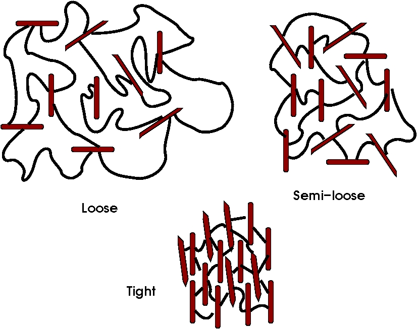
Fig. 2: Three types of actin network according to $\chi$. Reproduced from [13].

4.1 Parameters of the model and assumptions

We assume that the system is characterized by

1. The reference configuration $\Omega\subset{\mathbf{R}}^{3}$ and the previously defined positive quantities $L_{x}^{0}$, $\rho_{0}$, $\sigma_{x}^{0}$, $\chi$ and $A_{a}$.

2. The energy scaling parameters

   $$\mu=RT\sigma_{x}^{0},\quad\nu=RTA_{a}\rho_{0},$$ (78)

   where $R$ is the gas constant and $T$ the absolute temperature. In particular, they reflect the property that an increase in the rod aspect ratio, while holding the other parameters fixed, tends to favor nematic equilibrium.

Remark 4.

Since the rods are not randomly located in space as in the case of a fluid but serve as crosslink sites, $\rho_{0}$ and $L_{x}^{0}$ are not independent. For systems such that $L_{x}^{0}>>L_{a}$, the following estimate holds:

$$\rho_{0}=\frac{{\textrm{total volume of rods}}}{\textrm{total undeformed volume}}=K\frac{\chi^{3}}{\mathcal{A}_{a}^{2}}.$$ (79)

We have taken the material of the rod as having mass density 1. $K$ is a network constant that accounts for the number of crosslinks per actin unit and the coordination number of the network. Moreover, in estimating the denominator, we have assumed that the total volume of the system is fully spanned by the network.

4.1.1 Nematic rod fluid

We assume that $f:(-\frac{1}{2},1)\times(0,\infty)\longrightarrow\mathbf{R}$ represents a uniaxial bulk energy, parametrized by $\chi>0$, so that:

1. There exists a critical value $\chi_{t}$, such that, for $0<\chi<\chi_{t}$, $f$ has two local minima $\{s=0,\rho=\rho_{0}\}$ and $\{s^{*}>0,\rho^{*}>\rho_{0}\}$. For $\chi>\chi_{t}$, only the nematic minimum remains.

2. There exists a critical value $\chi_{l}<\chi_{t}$ such that,

   $$f(0,\rho_{0};\chi)<f(s^{*},\rho^{*};\chi),\quad{\textrm{ for}}\,\,0<\chi<\chi_{l},$$ (80)

   $$f(0,\rho_{0};\chi)>f(s^{*},\rho^{*};\chi),\quad{\textrm{for}}\,\,\chi_{l}<\chi<\chi_{t},$$ (81)

   $$f(0,\rho_{0};\chi_{l})=f(s^{*},\rho^{*};\chi_{l}).$$ (82)

3. $f(s^{*},\rho^{*};\chi)$ decreases with increasing $\chi$, and $s^{*}$ increases and $\rho^{*}$ decreases, also with respect to $\chi$.

4. $f$ has a maximum at $s=s^{**},\rho=\rho^{**}$, $0<s^{**}<s^{*},$ $\rho_{0}<\rho^{**}<\rho^{*}$.

5. It satisfies growth conditions with respect to $s$ and $\rho$:

   $$\lim_{s\to\{-\frac{1}{2},1\}}f(s,\rho;\chi)=+\infty,\,\textrm{for all}\,\,\rho>0,$$ (83)

   $$\lim_{\rho\to\{0,\infty\}}f(s,\rho;\chi)=+\infty,\,\textrm{ for all}\,s\in(-\frac{1}{2},1).$$ (84)

In the next section, we provide a method of construction a function $f$ satisfying these properties.

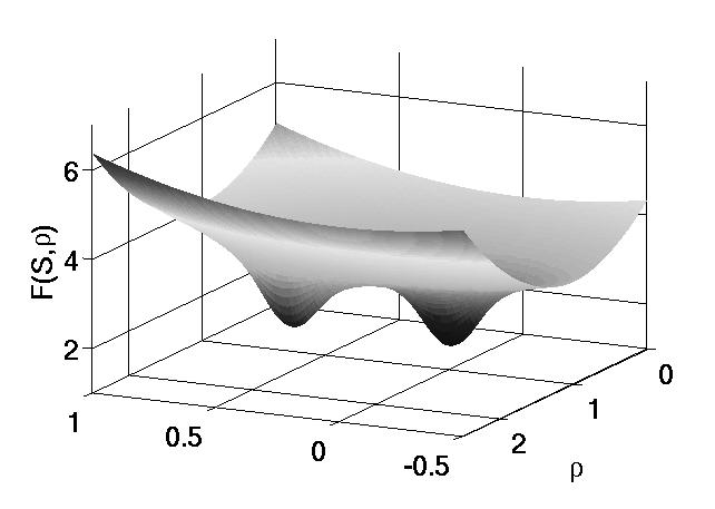
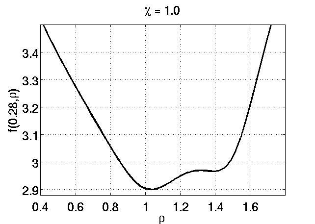
Fig. 3: 3D plot of the bulk free energy (left) and its corresponding cross section at $s=0.28$ (right) in the case $\chi=1.0$.

4.2 Density dependent phase transitions

Let us consider deformations with gradient

$$F=\mathop{\operator@font diag}\nolimits(\lambda,\lambda,\lambda),\quad\rho\lambda^{3}=\rho_{0}.$$ (85)

Set $\boldsymbol{n}_{0}=0$, choose $W=\mathcal{W}_{\textrm{\tiny{BTW}}}$ as in (27) and calculate the total energy density

$$\mathcal{E}:=\lambda^{3}\big{(}\mu(1-\alpha s^{2})+\nu f(s,\rho;\chi)\big{)}.$$ (86)

We consider $\mathcal{E}$ parametrized by $\rho$ and calculate the critical points

$$\frac{d\mathcal{E}}{ds}=\lambda^{3}\big{(}-2\alpha\mu s+\nu f_{s}(s,\rho;\chi)\big{)}=0.$$ (87)

We now discuss the solvability of the critical point equation as the parameter $\rho$ varies. In the case of multiple solutions, we choose that with the lowest energy. We summarize the results as follows.

Proposition 12.

Let $\rho_{0}>0$ be prescribed. Then the homogeneous minimizers of the energy have the following properties:

1. For $\chi\geq\chi_{t}$, the minimizer $s=s(\rho,A_{a},\chi)>0$ for all $\rho>0$ with $s(\rho,A_{a},\cdot)$ increasing and such that $s(\rho,A_{a},\chi)\to 1$ as $\chi\to\infty$.

2. For $0\leq\chi\leq\chi_{t}$, there exists a function $\rho=R(A_{a},\chi)$, decreasing as $A_{a}$ increases, with $\chi$ held fixed, and increasing as $\chi$ decreases, with $A_{a}$ held fixed, and such that the minimizers satisfy

   $$s(\rho,A_{a},\chi)>0,\,\,{\textrm{for}}\,\,\rho\geq R(A_{a},\chi),$$ (88)

   $$s(\rho,A_{a},\chi)\approx 0,\,\,{\textrm{for}}\,\,\rho<R(A_{a},\chi).$$ (89)

   Moreover, $R(A_{a},\chi)\to\infty$ as $\chi\to 0$. Furthermore, $s(\cdot,A_{a},\chi)$ may be discontinuous across $R(\cdot)$.

Comparing the liquid crystal behavior of the system under expansion with the next simulations on extension provides additional information on network effects.

4.2.1 Isotropic-Nematic Phase Transitions

We now carry out numerical simulations to describe the phase transition behavior under plane strain deformation given by

$$F=\mathop{\operator@font diag}\nolimits(\lambda,\lambda,1),\,\,\,\lambda^{2}\rho=\rho_{0}.$$ (90)

We present three types of plots: the phase diagrams (4) and (5) in the $(\rho,A_{a})$-plane, the graphs (LABEL:fig:lubinski-like) and (7) of the equilibrium order parameter $s$ in terms of the extension ratio $\lambda$, and the stress-strain diagrams (LABEL:fig:stress_strain_comparison).

The phase diagrams are obtained by solving the equation of critical points, that is, the analog of (87) and, in the case of multiple solutions, plotting that with smallest energy. Specifically, let us define, the isotropic $\mathcal{E}_{iso}=\mathcal{E}(s=0,\rho)$ and the nematic $\mathcal{E}_{nema}=\mathcal{E}(s\neq 0,\rho)$ energies, respectively. The construction of the phase diagrams is summarized as follows:

1. Construct the bulk energy function $f(s,\rho;\chi)$ for the problem.

2. Define a domain $\mathcal{B}=[\rho_{1},\rho_{2}]\times[A_{a1},A_{a2}]$ in the density-aspect-ratio space.

3. Choose a discrete subset $\mathcal{B}_{h}\subset\mathcal{B}$ such that,

   $$\mathcal{B}_{h} = \{(\rho_{1}+ih_{1},A_{a1}+jh_{2})\ |\ 0<h_{1}<(\rho_{2}-\rho_{1}),0<h_{2}<(A_{a2}-A_{a1})$$

   $$\&\ i,j\in\mathbb{N}\}.$$

4. Given a point $(\rho_{i},A_{ai})\in\mathcal{B}_{h}$ compute $s$ by solving the equilibrium equation $\frac{d\mathcal{E}}{ds}=0$.

5. The point $(\rho_{i},A_{ai})$ is labelled isotropic if $\mathcal{E}_{iso}<\mathcal{E}_{nema}$ and nematic otherwise.

6. Finally, we plot the nematic and isotropic points in a $(\rho,A_{a})$-diagram. We follow the convention of assigning red to nematic points, and blue to isotropic ones.

We construct $f$ as follows. Let $z:=\det F$, and define

$$h(s,z;\chi,s_{i,n},z_{i,n},\eta_{i,n}) = \chi W_{iso}(s,z;s_{i},z_{i},\eta_{i})+W_{nema}(s,z;s_{n},z_{n},\eta_{n})$$ (91)

$$+W_{gr}(s,z),$$

$$W_{iso}(s,z;s_{i},z_{i},\eta_{i}) = \arctan{\left(\eta_{i}((s-s_{i})^{2}+(z-z_{i})^{2})\right)}+(s-s_{i})^{2}$$ (92)

$$+(z-z_{i})^{2},$$

$$W_{nema}(s,z;s_{n},z_{n},\eta_{n}) = \arctan{\left(\eta_{n}((s-s_{n})^{2}+(z-z_{n})^{2}\right))},$$ (93)

$$W_{gr}(s,z) = -(\log(z)+\log(|s-1|(s+0.5))+z^{2}.$$ (94)

The parameters $s_{i,n},z_{i,n}$ represent the position of the isotropic and nematic minimum, respectively, and $\eta_{i,n}$ represent the width of the corresponding well. For a fixed set of parameters $\{s_{i,n},z_{i,n},\eta_{i,n}\}$, let

$$f(s,\rho;\chi)=h(s,z;\chi,s_{i,n},z_{i,n},\eta_{i,n}).$$ (95)

Figures 4 and 5 show phase diagrams for different values of $\chi$ and contour plots of $f(s,\rho;\chi)$. A main feature of these diagrams is that the density at which the nematic phase occurs increases with either lowering $\chi$ or $A_{a}$. (We hold $A_{a}$ fixed, in the first case, and $\chi$ in the latter). Moreover, in these diagrams, the isotropic phase is always present. It would require values $\chi>>10^{3}$ to encounter the nematic phase only. We stipulate that imposing a steeper growth of the energy with respect to $\rho$, for $\rho$ large, would also yield purely nematic phase diagrams for $\chi=O(10^{3})$.

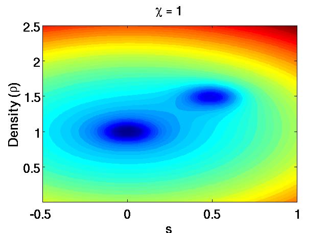
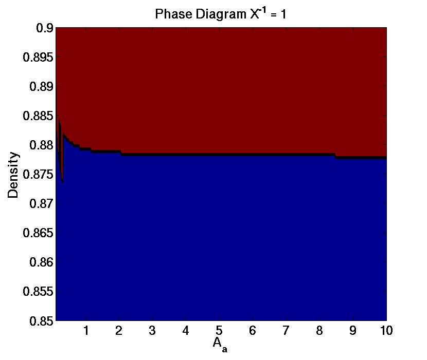
Fig. 4: Contour lines for the bulk potential function (left) and phase space diagram (right) for $\chi=1$.

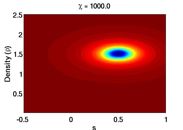
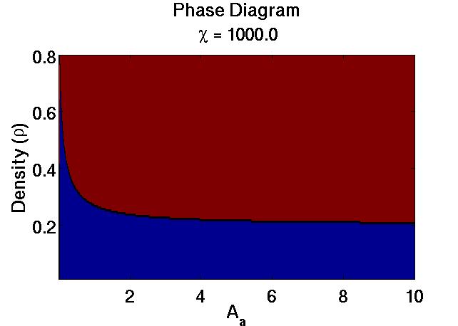
Fig. 5: Contour lines for the bulk potential function (left) and phase space diagram (right) $\chi=1000.0$.

4.2.2 Order Parameter Diagrams and Stress-Strain Plots

Figures 6 and 7 represent plots of the uniaxial order parameter $s$ with respect to the rod-density $\rho$, for $\chi=0.5,3.5,10$ and $80$, and for values of the aspect ratio $A_{a}$ ranging from $0.01$ to $80$. These values represent a range of shapes, from oblate cylinders to very elongated rods. The first graph in figure 4.5 presents two density-intervals with distinguished behavior, one corresponding to well aligned rods at high density, with a drop in the uniaxial order parameter as the density decreases to a critical value, and a second interval of further decrease in $s$ as $\rho$ continues decreasing. These graphs are in full agreement with those obtained by Montecarlo simulations in [6] and [13]. Moreover, the second graph of figure 4.5 and those in 4.6 present a third density interval of increase of the order parameter. This is due to the rod alignment that results from larger extension ratios (i.e., smaller densities), and it is a consequence of the elastic network connections of the rods. Proposition (4.1) shows that this behavior is not analytically predicted when subjecting the material to uniform expansion. It is not reported either in [13]. Another feature that emerges when comparing the two graphs on the right hand sides of figures 4.5 and 4.6 is that, for larger $\chi$, it requires to reach a lower density to increase the rod alignment. This may indicate the additional difficulty in aligning larger rods, in comparison with smaller ones.

We point out that the first graph in figure 7 shows the existence of oblate phases of rods with small aspect ratio, in the order of $10^{-2}$. This behavior is presented by cytoskeletal networks of red blood cells [3, 8, 30, 31].

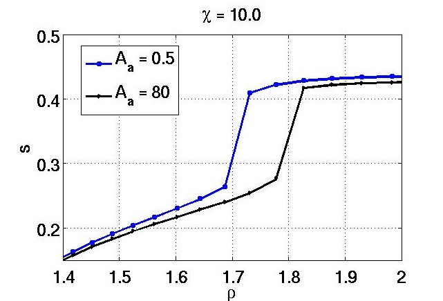
Fig. 6: Order parameter Vs density for $\chi=10$ (left) and $\chi=3.5$ (right). Nematic well: $s=0.5$, $\rho=1.5$.

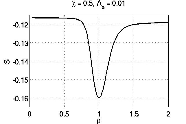
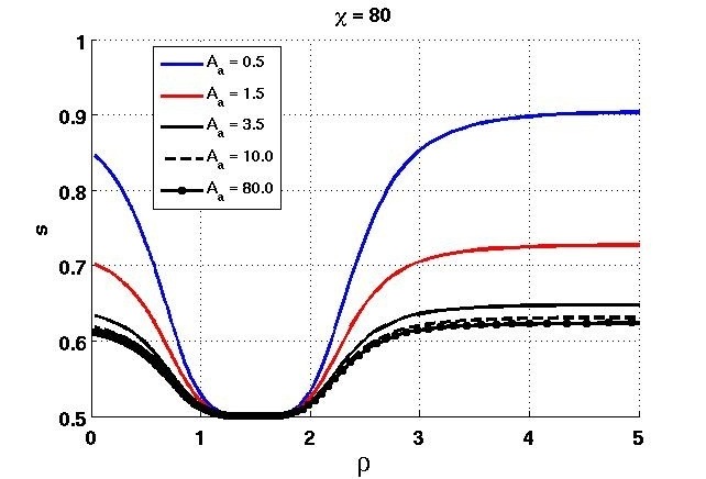
Fig. 7: Order parameter Vs density for $\chi=0.5$ (left) and $\chi=80$ (right). Nematic well: $s=0.5$, $\rho=0.5$.

We conclude this section discussing the stress-strain Figure LABEL:fig:stress_strain_comparison. For $\chi=0.5$ and for small and medium values of the rod aspect ratio, the stress-strain curves are monotonic and present a soft region followed by a steeper growth. However, we find that for $A_{a}=80$, the stress-strain curves are non-monotonic. The change of monotonicity occurs precisely where the order parameter experiences a sharp increase or decrease, indicating the change of volume accompanying rod order rearrangement. However, we also found shallower non-monotonic profiles, including for systems experiencing the nematic-isotropic phase transition, for aspect ratios smaller than 80. This seems to indicate that realignment of rods with large aspect ratio affects change of volume in a more significant way than for the smaller counterparts.

elastic part.

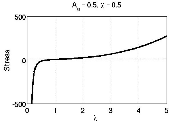
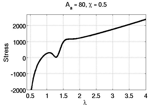
Fig. 8: Plots of the $xx$-components of the first Piola-Kirchhoff stress tensor.

5 Conclusions

We have presented and analyzed models of anisotropic elasticity based on the theory of liquid crystal elastomers, and applied them to modeling order phase transitions in actin networks.

We followed a strategy to show existence of minimizers based on the theory of isotropic nonlinear elasticity. This required assuming that the energy density function is polyconvex with respect to the anisotropic deformation tensor $G=L^{-\frac{1}{2}}\nabla\boldsymbol{\varphi}L_{0}^{\frac{1}{2}}$. The latter is at the core of the works on liquid crystal elastomers by Warner and Terentjev. An essential ingredient in the analysis is the assumption of a constitutive equation relating the shape of the polymer represented by the tensor $L$ with the order tensor $Q$ of the liquid crystal rigid units. The linear constitutive relation involves the restriction that both tensors become singular in the same region of the order parameter space. However, the linear relation implicitly involves the constraint of the trace of $L$ being constant, and therefore, it restricts the value of the sum of the principle axis of the ellipsoid associated with $L$. In future works, we will explore how to avoid this restriction by assuming nonlinear relations between the two tensors.

The assumptions on the bulk uniaxial free energy density function $f$, as well as the algorithm to generate specific forms of it, follow earlier works on uniaxial lyotropic liquid crystals. They also incorporate physically meaningful growth conditions required in the analysis. The results on phase transitions that we obtained from the proposed continuum theory show good agreement with those stemming from the molecular simulations that motivated this work, and from experimental results. In forthcoming work, we aim at constructing bulk free energy functions based on the Onsager rigid-rod theory. Although there is limited information on temperature dependence of the Landau-de Gennes energy for thermotropic nematic liquid crystals (22), the dependence on concentration in the lyotropic case seems to be lacking. In future work, we will also address the behavior of the system under shearing and consider the case of periodic crosslinking, also found in some actin networks.

6 Acknowledgment

This research was partially supported by a grant from the National Science Foundation, NSF-DMS 0909165.

References

- [1] Agostiniani, V. and DeSimone, A.:. Ogden-type energies for nematic elastomers. Int J. Nonlinear Mechanics, 47:402–412, 2012.
- [2] D. Anderson, D. Carlson, and E. Fried. A continuum-mechanical theory for nematic elastomers,. J. Elasticity, 56:33–58, 1999.
- [3] P. Bagchi and A.Z.K. Yazdani. Analysis of membrane tank-tread of nonspherical capsules and red blood cells. The European Physical Journal E, 35:1–12, 2012.
- [4] J.M. Ball. Convexity conditions and existence theorems in nonlinear elasticity. Archive for rational mechanics and Analysis, 63(4):337–403, 1976.
- [5] J.M. Ball and A. Majumdar. Nematic liquid crystals: from maier-saupe to a continuum theory. In Report no. OxPDE-10/10, 2010.
- [6] M.A. Bates and D. Frenkel. Phase behavior of two-dimensional hard rod fluids. J. Chem. Phys, 112(22):10034–10041, 2000.
- [7] MC Calderer and C. Liu. Liquid crystal flow: dynamic and static configurations. SIAM Journal on Applied Mathematics, 20:1225–1249, 2000.
- [8] Siqin Cao, Guanghong Wei, and Jeff Z. Y. Chen. Transformation of an oblate-shaped vesicle induced by an adhering spherical particle. Phys. Rev. E, 84:050901, Nov 2011.
- [9] P. Cesana and A. DeSimone. Strain-order coupling in nematic elastomers: equilibrium configurations. Math. Models Methods Appl. Sci, 19:601–630, 2009.
- [10] P. Cesana and A. DeSimone. Quasiconvex envelopes of energies for nematic elastomers in the small strain regime and applications. J. Mech. Phys. Solids, 59:787–803, 2011.
- [11] P.G. Ciarlet. Mathematical Elasticity, Vol 1. North-Holland, 1987.
- [12] S. Conti, A. DeSimone, and G. Dolzmann. Soft elastic response of stretched sheets of nematic elastomers: a numerical study. Journal of the Mechanics and Physics of Solids, 50(7):1431–1451, 2002.
- [13] P. Dalhaimer, D.E. Discher, and T.C. Lubensky. Crosslinked actin networks show liquid crystal elastomer behaviour, including soft-mode elasticity. Nature Physics, 3(5):354–360, 2007.
- [14] A. DeSimone and G. Dolzmann. Material instabilities in nematic elastomers . Physica D, 136(7):175–191, 2000.
- [15] A. DeSimone and G. Dolzmann. Macroscopic response of nematic elastomers via relaxation of a class of -invariant energies . Arch. Rat. Mech. Anal., 161(7):181–204, 2002.
- [16] A. DeSimone and L. Teresi. Elastic energies for nematic elastomers. The European Physical Journal E: Soft Matter and Biological Physics, 29(2):191–204, 2009.
- [17] JL Ericksen. Liquid crystals with variable degree of orientation. Archive for Rational Mechanics and Analysis, 113(2):97–120, 1991.
- [18] G. Forest, Q. Wang, and R. Zhou. A kinetic theory for solutions of nonhomogeneous nematic liquid crystalline polymers with density variations. J.Fluid Engineering, 126:180–188, 2004.
- [19] E. Fried and S Sellers. Free-energy density functions for nematic elastomers . J. Mech. Phys. Solids, 52:1671–1689, 1999.
- [20] E. Fried and S Sellers. Soft elasticity is not necessary for striping in nematic elastomers. Journal of Applied Physics, 100:043521–043325, 2006.
- [21] G. Friesecke, D.D. James, and S. Muller. A theorem on geometric rigidity and the derivation of nonlinear plate theory from three dimensional elasticity. Comm. Pure Appl. Math, 55:1461–1506, 2002.
- [22] F. Gamez, S. Lago, B. Garzon, P. Merklin, and C. Vega. Vapour-liquid equilibrium of fluids composed by oblate molecules. Molecular Physics, 106:1331–1339, 2008.
- [23] M. Gardel, Shin JH, Mahadevan L. MacKintosh FC, Matsudaira P., and Weitz DA. Elastic behavior of cross-linked and bundled actin networks. Science, 304:1301–1305, 2004.
- [24] E.F Gramsbergen, L Longa, and W.H. de Jeu. Landau theory of nematic isotropic phase transitions. Phys. Rep., 135:197–257, 1986.
- [25] R. Jerry, A. Popel, and W. Brownell. Outer hair cell length changes in an external electric field. i. the role of intracellular electro?osmotically generated pressure gradients. J.Accoustic Society of America, 98:2000–2010, 1995.
- [26] N. Kuzuu and M. Doi. Constitutive equation for nematic liquid crystals under weak velocity gradient derived from a molecular kinetic equation. I. J. Phys. Soc. Japan, 52:3486–3494, 1983.
- [27] N. Kuzuu and M. Doi. Constitutive equation for nematic liquid crystals under weak velocity gradient derived from a molecular kinetic equation. II. J. Phys. Soc. Japan, 53:1031–1040, 1984.
- [28] C Luo. Modeling, Analysis and Numerical Simulations of Liquid Crystal Elastomers, Ph.D dissertation, University of Minnesota, 2010.
- [29] A. Majumdar and A. Zarnescu. Landau–De Gennes Theory of Nematic Liquid Crystals: the Oseen–Frank Limit and Beyond. Archive for rational mechanics and analysis, 196(1):227–280, 2010.
- [30] C. Mohrdieck, F. Dalmas, E. Arzt, R. Tharmann, M. M. A. E. Claessens, A. R. Bausch, A. Roth, E. Sackmann, C. H. J. Schmitz, J. Curtis, W. Roos, K. Schulz, S.and Uhrig, and J. P. Spatz. Biomimetic models of the actin cytoskeleton. Small, 3(6):1015–1022, 2007.
- [31] C. Pozrikidis. The axisymmetric deformation of a red blood cell in uniaxial straining stokes flow. Journal of Fluid Mechanics, 216:231–254, 1990.
- [32] A.D. Rey. Liquid crystal models of biological materials and processes. Soft Matter, 6:3402–3429, 2010.
- [33] G.V. Richieri and S.P. Akeson. Measurement of biophysical properties of red blood cells by resistive pulse spectroscopy: volume, shape, surface area, and deformability. J. Biochem Biophys Methods, 11:117–131, 1985.
- [34] B. Wagner, R. Tharmann, I. Haase, M. Fischer, and A. R. Bausch. Cytoskeletal polymer networks: The molecule structure of cross-linkers determines macroscopic properties.cochlear outer hair-cells. Proc.Natl. Acad. Sci USA, 103:13974–13978, 2006.
- [35] M. Warner and E.M. Terentjev. Liquid crystal elastomers. Oxford University Press, USA, 2007.
- [36] B. Wincure and A.D. Rey. Growth regimes in phase ordering transformations. Discrete and Continous Dynamical Systems B, 8:623–648, 2007.