Surprising Asymptotic Conical Structure in Critical Sample Eigen-Directions

Abstract

The aim of this paper is to establish several deep theoretical properties of principal component analysis for multiple-component spike covariance models. Our new results reveal a surprising asymptotic conical structure in critical sample eigendirections under the spike models with distinguishable (or indistinguishable) eigenvalues, when the sample size and/or the number of variables (or dimension) tend to infinity. The consistency of the sample eigenvectors relative to their population counterparts is determined by the ratio between the dimension and the product of the sample size with the spike size. When this ratio converges to a nonzero constant, the sample eigenvector converges to a cone, with a certain angle to its corresponding population eigenvector. In the High Dimension, Low Sample Size case, the angle between the sample eigenvector and its population counterpart converges to a limiting distribution. Several generalizations of the multi-spike covariance models are also explored, and additional theoretical results are presented.

, , and

m1Corresponding Author t1Partially supported by NSF grant DMS-0854908 t2Partially supported by NSF grants DMS-1106912 and CMMI-0800575, NIH Challenge Grant 1 RC1 DA029425-01, and the Xerox Foundation UAC Award t3Partially supported by NIH grants RR025747-01, P01CA142538-01, MH086633, EB005149-01 and AG033387 t4Partially supported by NSF grants DMS-0606577 and DMS-0854908

1 Introduction

Principal Component Analysis (PCA) is one of the most important visualization and dimension reduction tools. The theoretical properties of PCA, including the sample eigenvalues, eigenvectors, and PC scores, have been widely studied in different settings, when the sample size and/or the dimension increase to infinity. For example, Anderson (1963) [1] studied such properties under the classical statistical setting with $n\rightarrow\infty$ and a fixed dimension $d$. Johnstone and Lu (2009) [9] explored such properties under the random matrix setting with sample size $n\rightarrow\infty$ and $d\sim n$. Jung and Marron (2009) [10] derived such properties in a High Dimension, Low Sample Size (HDLSS) context, with a fixed $n$ and $d\rightarrow\infty$. More recently, Fan et al. (2013) [7] considered scenarios where the first few leading eigenvalues increase to $\infty$ together with $d$. See additional theoretical results in [2, 3, 14, 15, 13, 12, 19, 4, 11, 17] and references therein.

Generally speaking, the existing results indicate that the behavior of PCA strongly depend on the relationship among three key quantities: the dimension, the sample size, and the spike sizes (the relative sizes of the population eigenvalues $\{\lambda_{j}\}$). For instance, Shen et al (2012) [17] systematically investigated the theoretical properties of the $j$-th sample eigenvector and eigenvalue as $d/(n\lambda_{j})\rightarrow 0$ or $\infty$. Specifically, as $d/(n\lambda_{j})\rightarrow 0$, the $j$-th sample eigenvector converges to the corresponding population eigenvector, whereas strong inconsistency follows as $d/(n\lambda_{j})\rightarrow\infty$.

An interesting open question is to investigate the asymptotic properties of PCA when $d/(n\lambda_{j})$ converges to a constant $c_{j}\in(0,\infty)$, which is the aim of this paper. A broad theoretical framework of PCA under a broad range of cases, from the classical, through random matrix theory, and on to HDLSS, is studied here. Firstly, we show a new instance of unexpected asymptotic behavior of sample eigenvectors. Specifically, the critical sample eigenvectors lie in a right circular cone around the corresponding population eigenvectors. Although these sample eigenvectors converge to the cone, their locations within the cone are random. The angles of these cones have an increasing order, which is driven by an increasing sequence of the ratios $c_{j}$. We suggest this is as surprising as the HDLSS geometric representation results discovered by Hall et al (2005) [8], and further developed by Yata and Aoshima (2012) [19].

Secondly, we further extend the new results to the multi-spike cases where the population eigenvalues are asymptotically indistinguishable. We study the angle between the corresponding sample eigenvectors and the subspace spanned by the indistinguishable population eigenvectors. In HDLSS contexts, the cone angles are always random variables, whereas such randomness disappears when the sample size increases. We also show that in HDLSS settings, the PC scores are not consistent even when the angles between the sample eigenvectors and their population counterparts converge to 0.

Next we introduce two illustrative examples to help understand the main theoretical results in the paper, where the eigenvalues are respectively asymptotically distinguishable (Example 1.1) and indistinguishable (Example 1.2). Our theorems are applicable to a much broader class of general spike models.

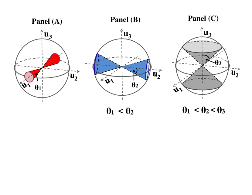
Figure 1: Geometric representation of PC directions in Example 1.1. The sphere represents the space of possible sample eigenvectors. Panel (A) shows that the first sample eigenvector tends to lie in the red cone, with the $\theta_{1}$ angle. Similarly, Panels (B) and (C) show that the second and the third sample eigenvectors respectively tend to lie in the blue and the gray cones, whose angles are $\theta_{2}$ and $\theta_{3}$. Note that the angle of the red cone is less than the blue cone, whose angle is again less than the gray cone.

Example 1.1.

(Multiple-component spike models with distinguishable eigenvalues) Assume that $X_{1},\ldots,X_{n}$ are random sample vectors from a $d$-dimensional normal distribution $N(0,\Sigma)$, where the population eigenvalues have the following properties: as $n\rightarrow\infty$,

$$\left\{\begin{array}[]{ll}\lambda_{1}>\lambda_{2}>\lambda_{3}\gg\lambda_{4}=\cdots=\lambda_{d}=1,\\ \frac{d}{n\lambda_{j}}\rightarrow c_{j},\quad j=1,2,3,\;\mbox{with}\;\;0\leq c_{1}<c_{2}<c_{3}\leq\infty.\end{array}\right.$$ (1.1)

In Figure 1, the sphere represents the space of all possible sample eigen-directions, with the first three population eigenvectors as the coordinate axes. For this particular example, our general Theorem 3.1 suggests that

• As $n\rightarrow\infty$, the sample eigenvector $\hat{u}_{1}$ lies in the red cone, shown in Panel (A) of Fig. 1, where the angle of the cone is $\theta_{1}=\arccos(\frac{1}{\sqrt{1+c_{1}}})$. Similarly, as $n\rightarrow\infty$, the sample eigenvectors $\hat{u}_{2}$ and $\hat{u}_{3}$ respectively lie in the blue and dark gray cones, shown in Panels (B) and (C) of Fig. 1, whereas the angles are respectively $\theta_{2}=\arccos(\frac{1}{\sqrt{1+c_{2}}})$ and $\theta_{3}=\arccos(\frac{1}{\sqrt{1+c_{3}}})$. Note that for $c_{1}<c_{2}<c_{3}$, we have $\theta_{1}<\theta_{2}<\theta_{3}$, as shown in Figure 1.

In addition, our Proposition 3.1 includes the two boundary cases studied by Shen et al. (2012) [17] as special cases:

• When $c_{1}=c_{2}=c_{3}=0$, it follows that $\theta_{1}=\theta_{2}=\theta_{3}=0$. This puts us in the domain of consistency [17].

• In the opposite boundary case of $c_{1}=c_{2}=c_{3}=\infty$, we have that $\theta_{1}=\theta_{2}=\theta_{3}=90$ degrees. This leads to strong inconsistency [17].

Hence, our new results go well beyond the work of [17], and completely characterize the transition between consistency and strong inconsistency.

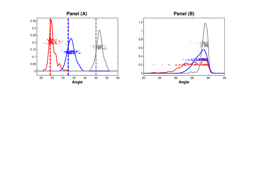
Figure 2: Example 1.1: Simulated angles between sample and population eigenvectors. Panel (A) shows realizations of angles between sample and population eigenvectors as colored dots (red is first, blue is second, gray is third). Distributions are studied using kernel density estimates, and compared with the theoretical values $\theta_{j}$ for $j=1,2,3$, shown as dashed lines. Panel (B) studies randomness of eigen-directions within the cones shown in Figure 1, by showing the distribution of pairwise angles between realizations of the sample eigenvectors. All 3 colors are overlaid here, and all angles are very close to 90 degrees, which is very consistent with the randomness of the respective sample eigenvectors within the cones.

We investigated this theoretical convergence, using simulations, over a range of settings, with $n=50,100,200,500,1000,2000$, where $d/n=50$, and $c_{1}=0.2,c_{2}=0.4,c_{3}=1$. The full sequence, illustrating this convergence, is shown in Figure A of the supplementary material [18]. Figure 2 shows the intermediate case of $n=200$. For one data set with this distribution, we compute angles between the sample and population eigenvectors. Repeating this procedure over 100 replications, we get 100 angles for each of the first three eigenvectors, which are shown as red, blue and gray points in Panel (A). The red, blue, gray curves are the corresponding kernel density estimates. Panel (A) shows that the simulated angles are very close to the corresponding theoretical angles $\theta_{j}$, $j=1,2,3$, shown as dashed vertical lines.

Panel (B) in Figure 2 studies randomness of eigen-directions within the cones shown in Figure 1. We calculate pairwise angles between realizations of the sample eigenvectors for the three cones, showing angles and kernel density estimates using colors as in Panel (A) of Figure 2. All angles are very close to 90 degrees, which is consistent with randomness in high dimensions, see [8, 19, 10, 11] and the more recent work of Cai et al. (2013) [6]. In fact, the regions represented by circles in Figure 1, are actually $d-1$ dimensional hyperspheres, so the sample eigenvectors should be thought of as d-1 dimensional as $d,n\rightarrow\infty$.

Example 1.2.

(Multiple-component spike models with indistinguishable eigenvalues) We again assume that $X_{1},\ldots,X_{n}$ are random sample vectors from a $d$-dimensional normal distribution $N(0,\Sigma)$. Different from Example 1.1, the six leading population eigenvalues of $\Sigma$ fall into three asymptotically separable pairs as follows: as $n\rightarrow\infty$

$$\left\{\begin{array}[]{ll}\lambda_{1}=\lambda_{2}>\lambda_{3}=\lambda_{4}>\lambda_{5}=\lambda_{6}\gg\lambda_{7}=\cdots=\lambda_{d}=1,\\ \frac{d}{n\lambda_{2j-1}}\rightarrow c_{j},\quad j=1,2,3,\;\mbox{with}\;\;0\leq c_{1}<c_{2}<c_{3}\leq\infty.\end{array}\right.$$

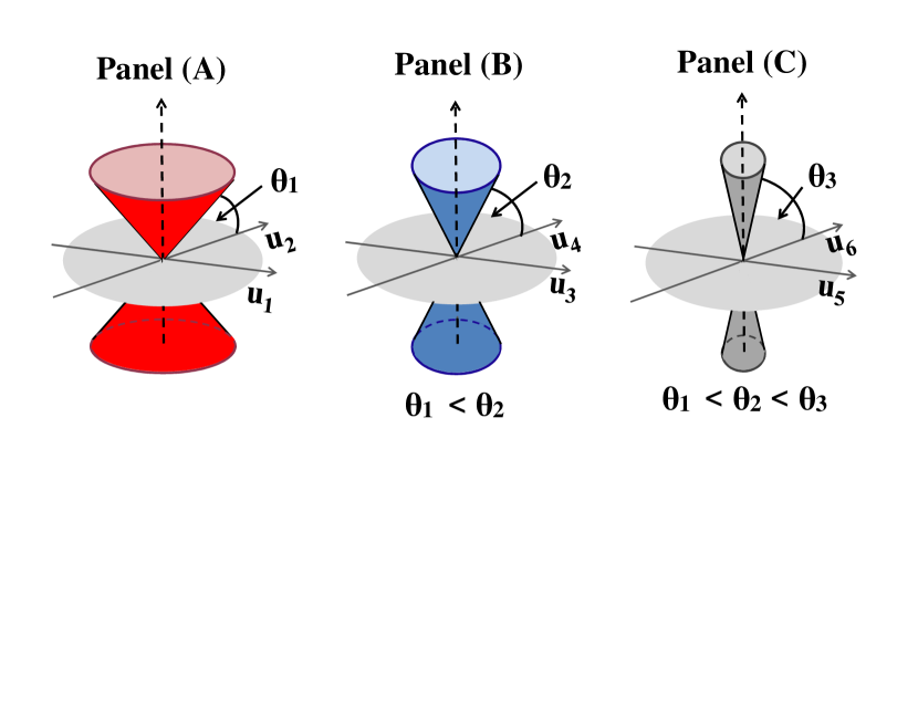
Figure 3: Example 1.2: Geometric representation of PC directions. Panel (A) shows the cone to which the first group of sample eigenvectors converge in the red. This cone has angle $\theta_{1}$ with the gray subspace, generated by the first group of population eigenvectors. Similarly, Panel (B) (Panel (C)) shows the cone to which the second (third) group of sample eigenvectors converges shown as a blue (dark gray) cone, which has angle $\theta_{2}$ ($\theta_{3}$) with the subspace, generated by the second (third) group of population eigenvectors.

Our general Theorem 3.2, when applied to the current example, reveals the following insights:

• Panel (A) in Figure 3 shows, as a red cone, the region where the first group of sample eigenvectors $\hat{u}_{1}$ and $\hat{u}_{2}$ lie in the limit as $n\rightarrow\infty$. This has the angle $\theta_{1}=\arccos(\frac{1}{\sqrt{1+c_{1}}})$ with the gray subspace, generated by the first group of population eigenvectors $u_{1}$ and $u_{2}$. Similarly, Panel (B) (Panel (C)) presents, as a blue (gray) cone, the region where the second (third) group of sample eigenvectors $\hat{u}_{3}$ and $\hat{u}_{4}$ ($\hat{u}_{5}$ and $\hat{u}_{6}$) lie in the limit as $n\rightarrow\infty$. This has the angle $\theta_{2}=\arccos(\frac{1}{\sqrt{1+c_{2}}})$ ($\theta_{3}=\arccos(\frac{1}{\sqrt{1+c_{3}}})$) with the subspace, generated by the second (third) group of population eigenvectors $u_{3}$ and $u_{4}$ ($u_{5}$ and $u_{6}$). Note that for $c_{1}<c_{2}<c_{3}$, we have $\theta_{1}<\theta_{2}<\theta_{3}$, as shown in Figure 3.

Furthermore, our Proposition B.1 in the supplementary document [18] considers boundary cases of our general framework, which includes the results of Shen et al. (2012) [17] as special cases:

• For $c_{1}=c_{2}=c_{3}=0$, it follows that $\theta_{1}=\theta_{2}=\theta_{3}=0$. This puts us in the domain of subspace consistency, as studied in Theorem 4.3 of [17].

• When $c_{1}=c_{2}=c_{3}=\infty$, we have that $\theta_{1}=\theta_{2}=\theta_{3}=90$ degrees. This leads to strong inconsistency, as studied in Theorem 4.3 of [17].

The rest of the paper is organized as follows. Section 2 introduces the assumptions and notation relevant to the theorems in the paper. Section 3 studies the asymptotic properties of PCA for multiple spike models with distinguishable (or indistinguishable) eigenvalues as $n\rightarrow\infty$. Section 4 studies the asymptotic properties of PCA in the HDLSS contexts. Section 5 contains the technical proofs of the main theorems. Additional simulation studies and proofs can be found in the supplementary document [18].

2 Assumptions and Notation

Let $X_{1},\ldots,X_{n}$ be random vectors from a $d$-dimensional normal distribution $N(\xi,\Sigma)$, where $\xi$ is a $d\times 1$ mean vector and $\Sigma$ is a $d\times d$ covariance matrix. Let $\{(\lambda_{k},u_{k}):k=1,\cdots,d\}$ be the eigenvalue-eigenvector pairs of $\Sigma$ such that $\lambda_{1}\geq\lambda_{2}\geq\ldots\geq\lambda_{d}>0$. Thus, $\Sigma$ has the following eigen-decomposition

$$\Sigma=U\Lambda U^{T},$$

where $\Lambda=\mbox{diag}(\lambda_{1},\ldots,\lambda_{d})$ and $U=[u_{1},\ldots,u_{d}]$. Since the relative sizes, rather than the absolute values, of the population eigenvalues affect the asymptotic properties of PCA, we assume that $\lambda_{d}=1$ throughout the rest of the paper.

Let $\overline{X}$ be the sample mean. As discussed in [16],

$$\sum_{i=1}^{n}(X_{i}-\overline{X})(X_{i}-\overline{X})^{T}\quad\mbox{has\;the\;same\;distribution\;as}\quad\sum_{i=1}^{n-1}Y_{i}Y_{i}^{T},$$ (2.1)

where $Y_{i}$ are i.i.d random vectors from $N(0,\Sigma)$. It follows from (2.1) that the sample covariance matrix is location invariant. Thus, we can assume without loss of generality (WLOG):

Assumption 2.1.

$X_{1},\ldots,X_{n}$ are i.i.d random vectors from a $d$-dimensional normal distribution $N(0,\Sigma)$.

Denote the $j$th normalized population PC score vector as

$$S_{j}=(S_{1,j},\cdots,S_{n,j})^{T}=\lambda_{j}^{-\frac{1}{2}}(u_{j}^{T}X_{1},\cdots,u_{j}^{T}X_{n})^{T},\quad j=1,\cdots,d,$$ (2.2)

and define $Z$ as the $n\times d$ random matrix as

$$Z=(z_{i,j})_{n\times d}=X^{T}U\Lambda^{-\frac{1}{2}},$$ (2.3)

where $X=[X_{1},\ldots,X_{n}]$ and $z_{i,j}$, $i=1,\cdots,n$, $j=1,\cdots,d$ are i.i.d random variables from $N(0,1)$.

Let $\{(\hat{\lambda}_{k},\hat{u}_{k}):k=1,\cdots,d\}$ be the eigenvalue-eigenvector pairs of the sample covariance matrix $\hat{\Sigma}=n^{-1}XX^{T}$ such that $\hat{\lambda}_{1}\geq\hat{\lambda}_{2}\geq\ldots\geq\hat{\lambda}_{d}$. Thus, $\hat{\Sigma}$ can be decomposed as

$$\hat{\Sigma}=\hat{U}\hat{\Lambda}\hat{U}^{T},$$ (2.4)

where $\hat{\Lambda}=\mbox{diag}(\hat{\lambda}_{1},\ldots,\hat{\lambda}_{d})$ and $\hat{U}=[\hat{u}_{1},\ldots,\hat{u}_{d}]$. Note that the data matrix $n^{-\frac{1}{2}}X$ has the singular value decomposition such that $n^{-\frac{1}{2}}X=\sum_{j=1}^{d}\hat{\lambda}_{j}^{\frac{1}{2}}\hat{u}_{j}\hat{v}^{T}_{j}$, where $\hat{v}_{j}=(\hat{v}_{1,j},\cdots,\hat{v}_{n,j})^{T}$ for $j=1,\cdots,d$. Thus, the $j$th normalized sample PC score vector is given by

$$\hat{S}_{j}=(\hat{S}_{1,j},\cdots,\hat{S}_{n,j})^{T}=(\hat{v}_{1,j},\cdots,\hat{v}_{n,j})^{T},\quad j=1,\cdots,d.$$ (2.5)

We introduce an asymptotic notation. Assume that $\{\xi_{k}:k=1,\ldots,\infty\}$ ($k=n$ or $d$) is a sequence of random variables and $\{e_{k}:k=1,\ldots,\infty\}$ is a sequence of constants. Denote $\xi_{k}={\rm O}_{\rm a.s}\left(e_{k}\right)$ if $\overline{\mbox{lim}}_{k\rightarrow\infty}\left|\frac{\xi_{k}}{e_{k}}\right|\leq\zeta$ almost surely with $P(0<\zeta<\infty)=1$ .

3 Growing sample size asymptotics

We now study asymptotic properties of PCA as $n\rightarrow\infty$. We consider multiple component spike models with distinguishable population eigenvalues in Section 3.1 and with indistinguishable eigenvalues in Section 3.2. Moreover, we vary $d$ from the classical $d$ fixed asymptotics, through the random matrix version with $d\sim n$, all the way to the high dimension medium sample size (HDMSS) asymptotics of Cabanski et al (2010) [5] and Yata and Aoshima (2012) [20] with $d\gg n\rightarrow\infty$.

3.1 Multiple component spike models with distinguishable eigenvalues

We consider multiple component spike models with $m$ dominating spikes where finite $m\in[1,n\wedge d]$. The population eigenvalues are assumed to satisfy the following two assumptions:

1. As $n\rightarrow\infty$, $\lambda_{1}>\cdots>\lambda_{m}\gg\lambda_{m+1}\rightarrow\cdots\rightarrow\lambda_{d}=1.$

2. ${\rm As}\;n\rightarrow\infty,\quad\frac{d}{n\lambda_{j}}\rightarrow c_{j},\quad{\rm where}\quad 0<c_{1}<\cdots<c_{m}<\infty.$

We first make several comments about Assumptions $\mathcal{A}1$ and $\mathcal{A}2$.

• Assumption $\mathcal{A}1$ includes two separate parts:

  1. The $\lambda_{1}>\cdots>\lambda_{m}$ part makes it possible to separately consider the first $m$ principle component signals and study the corresponding asymptotic properties.

  2. The $\lambda_{m}\gg\lambda_{m+1}\rightarrow\cdots\rightarrow\lambda_{d}=1$ enables clear separation of the signal (contained in the first $m$ components) from the noise (in the higher order components), which then helps to derive the asymptotic properties of the first $m$ sample eigenvalues, eigenvectors, and PC scores.

• Assumption $\mathcal{A}2$ is the critical case, in which the positive information and the negative are of the same order. In particular, increasing $n$ and the spike positively impacts the consistency of PCA, whereas increasing $d$ has a negative impact.

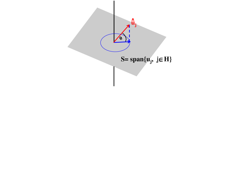
Figure 4: Angle between the sample eigenvector $\hat{u}_{j}$ and the space $\mathbb{S}$. The blue vector is the projection of the red vector $\hat{u}_{j}$ onto the space $\mathbb{S}$.

While the main focus of our results is the signal eigenvectors, some notation for the noise eigenvectors is also useful. According to Assumption $\mathcal{A}1$, the noise sample eigenvalues whose indices are greater than $m$ can not be asymptotically distinguished, so the corresponding eigenvectors should be treated as a whole. Therefore, we define the noise index set $H=\{m+1,\cdots,d\}$, and denote the space spanned by these noise eigenvectors as

$$\mathbb{S}=\mbox{span}\{u_{j},j\in H\}.$$ (3.1)

For each sample eigenvector $\hat{u}_{j}$, $j\in H$, we study the angle between $\hat{u}_{j}$ and the space $\mathbb{S}$, as defined in [10, 17] and illustrated in Figure 4, i.e. the angle between $\hat{u}_{j}$ (the red vector) and its projection onto $\mathbb{S}$ (the blue vector).

The following theorem derives the asymptotic properties of the first $m$ sample eigenvalues and eigenvectors. In addition, the theorem also shows that, for $j=m+1,\cdots,[n\wedge d]$, the angle between $\hat{u}_{j}$ and $u_{j}$ goes to 90 degrees, whereas the angle between $\hat{u}_{j}$ and the space $\mathbb{S}$ goes to 0.

Theorem 3.1.

Under Assumptions 2.1, $\mathcal{A}1$, and $\mathcal{A}2$, as $n\rightarrow\infty$, the sample eigenvalues satisfy

$$\left\{\begin{array}[]{ll}\frac{\hat{\lambda}_{j}}{\lambda_{j}}\xrightarrow{\rm a.s}1+c_{j},\;1\leq j\leq m,\\ \frac{n\hat{\lambda}_{j}}{d\lambda_{j}}\xrightarrow{\rm a.s}1,\;m+1\leq j\leq[n\wedge d],\\ \end{array}\right.$$ (3.2)

and the sample eigenvectors satisfy

$$\left\{\begin{array}[]{lll}\mid<\hat{u}_{j},u_{j}>\mid\xrightarrow{a.s}(1+c_{j})^{-\frac{1}{2}},\quad 1\leq j\leq m,\\ \mid<\hat{u}_{j},u_{j}>\mid={\rm O}_{\rm a.s}\left\{(\frac{n}{d})^{\frac{1}{2}}\right\},\quad m+1\leq j\leq[n\wedge d],\\ \mbox{angle}<\hat{u}_{j},\mathbb{S}>\xrightarrow{a.s}0,\quad m+1\leq j\leq[n\wedge d].\end{array}\right.$$ (3.3)

We now offer several remarks regarding Theorem 3.3.

Remark 3.1.

The results of (3.2) and (3.3) suggest that, as the eigenvalue index increases, the proportional bias between the sample and population eigenvalue increases, so the angle between the sample and corresponding population eigenvectors increases. This is because larger eigenvalues (i.e. with small indices) contain more positive information, which makes the corresponding sample eigenvalues/eigenvectors less biased. These results are graphically illustrated in Figure 1 and empirically verified in Figure 2, for the specific model in Example 1.1. More empirical support is provided in the supplementary material [18].

Remark 3.2.

Theorem 3.3 can be extended to include the classical and random matrix cases, by allowing $c_{m_{0}}=0$ for some $m_{0}\leq m$, which suggests that positive information dominates in the leading $m_{0}$ spikes. Then Assumptions $\mathcal{A}1$ and $\mathcal{A}2$ respectively become

1. as $n\rightarrow\infty$, the population eigenvalues satisfy

   $$\lambda_{1}>\cdots>\lambda_{m_{0}}\gg\lambda_{m_{0}+1}>\cdots>\lambda_{m}\gg\lambda_{m+1}\rightarrow\cdots\rightarrow\lambda_{d}=1.$$

2. as $n\rightarrow\infty$, $d/(n\lambda_{j})\rightarrow c_{j}$ for $j=1,\cdots,m$, where $0=c_{1}=\cdots=c_{m_{0}}<c_{m_{0}+1}<\cdots<c_{m}<\infty$.

For the classical case with fixed dimension $d$, $m_{0}=m=d$ in Assumptions $\mathcal{A}3$ and $\mathcal{A}4$. For random matrix cases with $n\sim d$, $m_{0}=m$ in Assumptions $\mathcal{A}3$ and $\mathcal{A}4$. Since $c_{1}=\cdots=c_{m_{0}}=0$ in Assumption $\mathcal{A}3$, if the eigenvalue index is less than or equal to $m_{0}$, the corresponding sample eigenvalues and eigenvectors are consistent. These results are summarized in the following Proposition 3.1(a).

Remark 3.3.

Another extension of Theorem 3.3 is to allow $c_{m_{0}+1}=\infty$ for some $m_{0}\leq m$, i.e. negative information dominates in higher-order spikes. This contains the HDMSS cases [5, 20], where $d\gg n\rightarrow\infty$. Assumption $\mathcal{A}1$ then becomes Assumption $\mathcal{A}3$, and Assumption $\mathcal{A}2$ becomes

1. as $n\rightarrow\infty$, $d/(n\lambda_{j})\rightarrow c_{j}$ for $j=1,\cdots,m$, where $0<c_{1}<\cdots<c_{m_{0}}<c_{m_{0}+1}=\cdots=c_{m}=\infty$.

Since $c_{m_{0}+1}=\cdots=c_{m}=\infty$, for index $j\geq m_{0}+1$, the proportional error between the sample and population eigenvalues goes to infinity, and the angle between the corresponding sample and population eigenvectors converges to 90 degrees. These results are summarized in Proposition 3.1(b).

Proposition 3.1.

1. Under Assumptions 2.1, $\mathcal{A}3$ and $\mathcal{A}4$, the sample eigenvalues and eigenvectors satisfy

   $$\hat{\lambda}_{j}/\lambda_{j}\quad\mbox{and}\quad\mid<\hat{u}_{j},u_{j}>\mid\quad\xrightarrow{a.s}1,\quad 1\leq j\leq m_{0},$$

   and the properties of the other sample eigenvalues and eigenvectors remain the same as in Theorem 3.3.

2. Let $H=\{m_{0}+1,\cdots,d\}$ and define $\mathbb{S}$ as in (3.1). If Assumption $\mathcal{A}4$ in (a) is replaced by Assumption $\mathcal{A}5$, the sample eigenvalues satisfy

   $$n\hat{\lambda}_{j}/d\xrightarrow{\rm a.s}1,\quad m_{0}+1\leq j\leq m,$$

   and the sample eigenvectors satisfy

   $$\left\{\begin{array}[]{ll}\mid<\hat{u}_{j},u_{j}>\mid={\rm O}_{\rm a.s}\left\{(\frac{n\lambda_{j}}{d})^{\frac{1}{2}}\right\},\\ \mbox{angle}<\hat{u}_{j},\mathbb{S}>\xrightarrow{a.s}0,\\ \end{array}\right.\quad m_{0}\leq j\leq[n\wedge d];$$

   the properties of the other sample eigenvalues and eigenvectors remain the same as in Theorem 3.3.

3. In addition, if Assumption $\mathcal{A}4$ in (a) is strengthened to $d/\lambda_{m_{0}}\rightarrow 0$, then the sample PC scores satisfy

   $$\left|\frac{\hat{S}_{i,j}}{S_{i,j}}\right|\xrightarrow{a.s}1,\quad i=1,\cdots n,\;j=1,\cdots,m_{0}.$$

3.2 Multiple component spike models with indistinguishable eigenvalues

We now consider spike models with the $m$ leading eigenvalues being grouped into $r$($\geq 1$) tiers, each of which contains eigenvalues that are either the same or have the same limit. The eigenvalues within different tiers have different limits. Specifically, the first $m$ eigenvalues are grouped into $r$ tiers, in which there are $q_{k}$ eigenvalues in the $k$th tier such that $\sum_{l=1}^{r}q_{l}=m$. Define $q_{0}=0$, $q_{r+1}=d-\sum_{l=1}^{r}q_{l}$, and the index set of the eigenvalues in the $k$th tier as

$$H_{k}=\left\{\sum_{l=0}^{k-1}q_{l}+1,\sum_{l=0}^{k-1}q_{l}+2,\cdots,\sum_{l=0}^{k-1}q_{l}+q_{k}\right\},\quad k=1,\cdots,r+1.$$ (3.4)

We make the following assumptions on the tiered eigenvalues:

1. The eigenvalues in the $k$th tier have the same limit $\delta_{k}(>0)$:

   $$\mbox{lim}_{n\rightarrow\infty}\frac{\lambda_{j}}{\delta_{k}}=1,\quad j\in H_{k},\;k=1,\cdots,r.$$

2. The eigenvalues in different tiers have different limits:

   $${\rm as}\;n\rightarrow\infty,\;\quad\delta_{1}>\cdots>\delta_{r}\gg\lambda_{m+1}\rightarrow\cdots\rightarrow\lambda_{d}=1.$$

3. The ratio between the dimension and the product of the sample size with eigenvalues in the same tier converges to a constant:

   $${\rm as}\;n\rightarrow\infty,\quad\frac{d}{n\delta_{k}}\rightarrow c_{k},\quad{\rm with}\quad 0<c_{1}<\cdots<c_{r}<\infty.$$

Assumptions $\mathcal{B}2$ and $\mathcal{B}3$ are natural extensions of Assumptions $\mathcal{A}1$ and $\mathcal{A}2$. In Assumption $\mathcal{B}2$, the signal contained in the first $r$ tiers of eigenvalues is well separated from the noise, and hence the asymptotic properties of the sample eigenvalues and eigenvectors in the first $r$ tiers can be obtained. Assumption $\mathcal{B}3$ suggests that the positive information (sample size and spike size) and the negative information (dimension) are of the same order.

Since the sample eigenvalues within the same tier can not be asymptotically identified, the corresponding sample eigenvectors are indistinguishable. For $j\in H_{k}$, in order to study the asymptotic properties of the sample eigenvector $\hat{u}_{j}$, we consider the angle between $\hat{u}_{j}$ and the subspace spanned by the population eigenvectors $u_{j}$ in the same tier, defined as

$$\mathbb{S}_{k}=\mbox{span}\{u_{j},j\in H_{k}\}.$$ (3.5)

Our theoretical results are summarized in the following theorem.

Theorem 3.2.

Under Assumptions 2.1, $\mathcal{B}1$, $\mathcal{B}2$ and $\mathcal{B}3$, as $n\rightarrow\infty$, the sample eigenvalues satisfy

$$\left\{\begin{array}[]{ll}\frac{\hat{\lambda}_{j}}{\lambda_{j}}\xrightarrow{\rm a.s}1+c_{k},\quad j\in H_{k},\;k=1,\cdots,r,\\ \frac{n\hat{\lambda}_{j}}{d\lambda_{j}}\xrightarrow{\rm a.s}1,\quad m+1\leq j\leq[n\wedge d],\\ \end{array}\right.$$ (3.6)

and the sample eigenvectors satisfy

$$\left\{\begin{array}[]{lll}\mbox{angle}<\hat{u}_{j},\mathbb{S}_{k}>\xrightarrow{a.s}\arccos\left\{(1+c_{k})^{-\frac{1}{2}}\right\},\;j\in H_{k},\;k=1,\cdots,r,\\ \mid<\hat{u}_{j},u_{j}>\mid={\rm O}_{\rm a.s}\left\{(\frac{n}{d})^{\frac{1}{2}}\right\},\quad m+1\leq j\leq[n\wedge d],\\ \mbox{angle}<\hat{u}_{j},\mathbb{S}_{r+1}>\xrightarrow{a.s}1,\quad m+1\leq j\leq[n\wedge d].\end{array}\right.$$ (3.7)

Theorem 3.2 is an extension of Theorem 3.3. For higher-order eigenvalues, the sample eigenvalues are more biased, while the angles between the sample eigenvectors and the subspaces spanned by their population counterparts in the same tiers are larger. See Figure 3 for an illustration of the specific model considered in Example 1.2. Theorem 3.2 can be extended to cover the classical, random matrix, and HDMSS cases, which is done in Section B of the supplementary material [18].

4 High dimension, low sample size asymptotics

We now study the asymptotic properties of PCA in the HDLSS context. In this case, the ratios between the sample eigenvalues and their population counterparts converge to non degenerate random variables, as do the angles between the sample eigenvectors and the space spanned by the corresponding population eigenvectors. This phenomenon of random limits does not exist when $n$ increases to $\infty$ as shown in Section 3.

Since the sample size is fixed, we can not distinguish the two types of spike models considered respectively in Sections 3.1 and 3.2. Hence, we merge the model assumptions there into the following corresponding assumptions:

1. For fixed $n$, as $d\rightarrow\infty$, $\lambda_{1}\geq\cdots\geq\lambda_{m}\gg\lambda_{m+1}\rightarrow\cdots\rightarrow\lambda_{d}=1$.

2. For fixed $n$, as $d\rightarrow\infty$,

   $$\frac{d}{n\lambda_{j}}\rightarrow c_{j},\quad\quad{\rm with}\quad 0<c_{1}\leq\cdots\leq c_{m}<\infty.$$

In particular, Assumption $\mathcal{C}1$ is parallel to Assumptions $\mathcal{A}1$, $\mathcal{B}1$ and $\mathcal{B}2$, while Assumption $\mathcal{C}2$ corresponds to Assumptions $\mathcal{A}2$ and $\mathcal{B}3$.

As stated below in Theorem 4.1, the sample eigenvalues and eigenvectors converge to non-degenerate random variables rather than constants. We define several quantities in order to describe the limiting random variables. Define the $m\times d$ matrix

$$\mathbb{M}=[\mathbb{C},0_{m\times(d-m)}]_{m\times d},\quad$$

where $\mathbb{C}=\mbox{diag}\{{c^{-1/2}_{1}},\cdots,{c^{-1/2}_{m}}\}$ is an $m\times m$ diagonal matrix and $0_{m\times(d-m)}$ is the $m\times(d-m)$ zero matrix. In addition, define the random matrix $\mathcal{W}$ as

$$\mathcal{W}=\mathbb{M}Z^{T}Z\mathbb{M}^{T},$$ (4.1)

where $Z$ is defined in (2.3). The eigenvalues of the random matrix $\mathcal{W}$ appear in the random limits of Theorem 4.1, as in (4.2) and (4.3).

Given the fixed sample size, the sample eigenvalues can not be asymptotically distinguished, nor can the corresponding sample eigenvectors. To study the asymptotic behavior of the sample eigenvectors, we need to consider the space $\mathbb{S}_{k}$ spanned by the corresponding population eigenvectors, as defined in (3.5), with the two index sets being $H_{1}=\left\{1,\cdots,m\right\}$ and $H_{2}=\left\{m+1,\cdots,d\right\}$.

We are now ready to state the main theorem in the HDLSS contexts.

Theorem 4.1.

Under Assumptions 2.1, $\mathcal{C}1$ and $\mathcal{C}2$, for fixed $n$, as $d\rightarrow\infty$, the sample eigenvalues satisfy

$$\left\{\begin{array}[]{ll}\frac{\hat{\lambda}_{j}}{\lambda_{j}}\xrightarrow{\rm a.s}\frac{c_{j}}{n}\lambda_{j}(\mathcal{W})+c_{j},\quad 1\leq j\leq m,\\ \frac{n\hat{\lambda}_{j}}{d\lambda_{j}}\xrightarrow{\rm a.s}1,\quad m+1\leq j\leq n,\\ \end{array}\right.$$ (4.2)

where $\mathcal{W}$ is defined in (4.1), and the sample eigenvectors satisfy

$$\left\{\begin{array}[]{lll}\mbox{angle}<\hat{u}_{j},\mathbb{S}_{1}>\xrightarrow{a.s}\arccos\left\{\left(1+\frac{n}{\lambda_{j}(\mathcal{W})}\right)^{-\frac{1}{2}}\right\},\quad 1\leq j\leq m,\\ \mid<\hat{u}_{j},u_{j}>\mid={\rm O}_{\rm a.s}(d^{-\frac{1}{2}}),\quad m+1\leq j\leq n,\\ \mbox{angle}<\hat{u}_{j},\mathbb{S}_{2}>\xrightarrow{a.s}1,\quad m+1\leq j\leq n.\end{array}\right.$$ (4.3)

Three remarks are offered below regarding Theorem 4.1.

Remark 4.1.

If $m=1$ in Theorem 4.1, i.e. for single-component spike models, then the first sample eigenvalue and eigenvector satisfy

$$\left\{\begin{array}[]{ll}\frac{\hat{\lambda}_{1}}{\lambda_{1}}\xrightarrow{a.s}\frac{\chi_{n}^{2}}{n}+c_{1},\\ \mid<\hat{u}_{1},u_{1}>\mid\xrightarrow{a.s}\left(1+\frac{nc_{1}}{\chi_{n}^{2}}\right)^{-\frac{1}{2}},\end{array}\right.$$

where $\chi_{n}^{2}$ is the Chi-square distribution with $n$ degrees of freedom. This result is consistent with Theorem 1 of Jung et al. (2012) [11].

Remark 4.2.

For $1\leq j\leq m$, as the relative size of the eigenvalue decreases, the angle between $\hat{u}_{j}$ and $\mathbb{S}_{1}$ increases. However, this phenomenon is not as strong as in the growing sample size settings studied in Section 3, where the sample eigenvectors can be separately studied, and the corresponding angles have a non-random increasing order.

Remark 4.3.

Assumption $\mathcal{C}2$ can be relaxed to include boundary cases, in which there exists an integer $m_{0}\in[1,m]$ such that $c_{m_{0}}=0$, i.e. positive information dominates in the leading $m_{0}$ spikes; or $c_{m_{0}+1}=\infty$, i.e. negative information dominates in the remaining high-order spikes. These theoretical results are presented in Section C of the supplementary material [18].

5 Proofs

We now provide some proofs of our theorems as $n\rightarrow\infty$. For the sake of space, we only present detailed proof for the properties of the sample eigenvectors here, which is the most challenging part. In contrast to showing consistency or inconsistency of the sample eigenvector, this proof requires precise calculation of the degree of inconsistency, i.e. the limiting angles between the sample and population eigenvectors. We relegate the derivations regarding the sample eigenvalues to Section D of the supplementary material [18], which also contains proofs of Proposition 3.1, Theorem 4.1, as well as extensions of Theorems 3.2 and 4.1.

The critical ideas of the proof are to first partition the sample eigenvector matrix $\hat{U}$ into sub-matrices, corresponding to the group index $H_{k}$. Then through careful analysis, we explore the connections between sample eigenvectors and eigenvalues and then use the sample eigenvalue properties to study the asymptotic properties of the sample eigenvectors.

WLOG, we assume that $\lambda_{m+1}=\cdots=\lambda_{d}=1$. Due to the invariance property of the angle between the sample and population eigenvectors, see Shen et al. (2012) [17], we assume WLOG that the population eigenvectors $u_{j}=e_{j}$, $j=1,\ldots,d$, where the $j$-th component of $e_{j}$ equals 1 and the rest are zero. It follows that the inner product between the sample and population eigenvectors satisfies

$$\mid<\hat{u}_{j},u_{j}>\mid^{2}=\mid<\hat{u}_{j},e_{j}>\mid^{2}=\hat{u}^{2}_{j,j},$$

and the angle between the sample eigenvector and the corresponding population subspace $\mathbb{S}_{k}$ in (3.5) satisfies

$$\left(\mbox{cos}\left[\mbox{angle}\left(\hat{u}_{j},\mathbb{S}_{k}\right)\right]\right)^{2}=\sum_{l\in H_{k}}\hat{u}^{2}_{l,j},\quad k=1,\cdots,r+1.$$ (5.1)

The population eigenvalues are grouped into $r+1$ tiers and $H_{k}$ in (3.4) is the index set of the eigenvalues in the $k$th tier. Define

$$\hat{U}_{k,l}=(\hat{u}_{i,j})_{i\in H_{k},j\in H_{l}},\quad 1\leq k,l\leq r+1.$$

Then, the sample eigenvector matrix $\hat{U}$ can be expressed as:

$$\hat{U}=[\hat{u}_{1},\hat{u}_{2},\cdots,\hat{u}_{d}]=\begin{pmatrix}\hat{U}_{1,1}&\hat{U}_{1,2}&\cdots&\hat{U}_{1,r+1}\\ \hat{U}_{2,1}&\hat{U}_{2,2}&\cdots&\hat{U}_{2,r+1}\\ \vdots&\vdots&&\vdots\\ \hat{U}_{r+1,1}&\hat{U}_{r+1,2}&\cdots&\hat{U}_{r+1,r+1}\end{pmatrix}.$$ (5.2)

The proof of the asymptotic properties of the sample eigenvectors (3.7) depends on the asymptotic properties of the sample eigenvalues, as stated in (3.6) of Theorem 3.2, which are derived in the supplementary material [18]. The following proof considers two groups of sample eigenvectors separately. Section 5.1 obtains the asymptotic properties for the sample eigenvectors whose index is greater than $m$. Section 5.2 derives asymptotic properties for the sample eigenvectors whose index is less than or equal to $m$.

5.1 Asymptotic properties of the sample eigenvectors $\hat{u}_{j}$ with $j>m$

We derive the asymptotic properties through the following two steps:

• First, we show that as $n\rightarrow\infty$, the angle between $\hat{u}_{j}$ and $u_{j}$ converges to 90 degrees:

  $$\mid<\hat{u}_{j},u_{j}>\mid^{2}=\hat{u}^{2}_{j,j}={\rm O}_{\rm a.s}\left(\frac{n}{d}\right),\quad j=m+1,\cdots,[n\wedge d].$$ (5.3)

• Then, we show that as $n\rightarrow\infty$, the angle between $\hat{u}_{j}$ and the corresponding subspace $\mathbb{S}_{r+1}$ converges to 0, where $\mathbb{S}_{r+1}$ is defined as in (3.5):

  $$\mbox{angle}<\hat{u}_{j},\mathbb{S}_{r+1}>\xrightarrow{a.s}0,\quad j=m+1,\cdots,[n\wedge d].$$ (5.4)

We now provide the proof for the first step. Denote $W=\Lambda^{-\frac{1}{2}}\hat{U}\hat{\Lambda}^{\frac{1}{2}}$, where $\hat{U}$ is the sample eigenvector matrix and $\hat{\Lambda}$ is the sample eigenvalue matrix defined in (2.4). It follows from (2.3) and (2.4) that $WW^{T}=\frac{1}{n}ZZ^{T}$, where $Z$ is defined in (2.3). Considering the $k$-th diagonal entry of the two equivalent matrices $WW^{T}$ and $\frac{1}{n}ZZ^{T}$, and noting that $w_{k,j}=\lambda^{-\frac{1}{2}}_{k}\hat{\lambda}^{\frac{1}{2}}_{j}\hat{u}_{k,j}$, it follows that

$$\lambda^{-1}_{k}\sum_{j=1}^{d}\hat{\lambda}_{j}\hat{u}^{2}_{k,j}=\sum_{j=1}^{d}w^{2}_{k,j}=\frac{1}{n}\sum_{i=1}^{n}z^{2}_{i,k}.\quad k=1,\cdots,d.$$ (5.5)

In addition, note that $\frac{1}{n}\sum_{i=1}^{n}z^{2}_{i,k}\xrightarrow{\rm a.s}1$, as $n\rightarrow\infty$, and $\hat{\lambda}_{j}=0$ for $j>[n\wedge d]$. Combining the above with (5.5), we obtain that

$$\sum_{l=1}^{r}\sum_{j\in H_{l}}\lambda^{-1}_{k}\hat{\lambda}_{j}\hat{u}^{2}_{k,j}+\sum_{j=m+1}^{[n\wedge d]}\lambda^{-1}_{k}\hat{\lambda}_{j}\hat{u}^{2}_{k,j}\xrightarrow{a.s}1,\quad k=1,\cdots,d.$$ (5.6)

Furthermore, it follows from (5.6) that as $n\rightarrow\infty$,

$$\hat{u}^{2}_{j,j}\stackrel{{\scriptstyle\rm a.s}}{{\leq}}\frac{\lambda_{j}}{\hat{\lambda}_{j}},\quad j=m+1,\cdots,[n\wedge d],$$ (5.7)

which, together with the asymptotic properties of the sample eigenvalues (3.6), yields (5.3).

We then move on to prove the second step. According to (5.1), we need to show that

$$\sum_{k=m+1}^{d}\hat{u}^{2}_{k,j}\xrightarrow{a.s}1,\quad j=m+1,\cdots,[n\wedge d].$$ (5.8)

The non-zero $k$-th diagonal entry of $W^{T}W$ is between its smallest and largest eigenvalues. Since $W^{T}W$ shares the same non-zero eigenvalues as $\frac{1}{n}Z^{T}Z$, it follows that for $j=1,\cdots,[n\wedge d]$,

$$\lambda_{\mbox{min}}(\frac{1}{n}Z^{T}Z)\leq\hat{\lambda}_{j}\sum_{k=1}^{d}\lambda^{-1}_{k}\hat{u}^{2}_{k,j}=\sum_{k=1}^{d}w^{2}_{k,j}\leq\lambda_{\mbox{max}}(\frac{1}{n}Z^{T}Z),$$ (5.9)

which yields that, for $j=m+1,\cdots,[n\wedge d]$,

$$\frac{\lambda_{j}}{\hat{\lambda}_{j}}\lambda_{\mbox{min}}(\frac{1}{n}Z^{T}Z)\leq\sum_{k=1}^{d}\lambda_{j}\lambda^{-1}_{k}\hat{u}^{2}_{k,j}\leq\frac{\lambda_{j}}{\hat{\lambda}_{j}}\lambda_{\mbox{max}}(\frac{1}{n}Z^{T}Z).$$ (5.10)

According to Lemma D.1 in the supplementary material [18] and the asymptotic properties of the sample eigenvalues (3.6), we have that, for $j=m+1,\cdots,[n\wedge d]$,

$$\frac{\lambda_{j}}{\hat{\lambda}_{j}}\lambda_{\mbox{min}}\left(\frac{1}{n}Z^{T}Z\right)\quad\mbox{and}\quad\frac{\lambda_{j}}{\hat{\lambda}_{j}}\lambda_{\mbox{max}}\left(\frac{1}{n}Z^{T}Z\right)\quad\xrightarrow{a.s}1.$$ (5.11)

In addition, it follows from Assumption $\mathcal{B}2$ that, for $j=m+1,\cdots,[n\wedge d]$,

$$\left\{\begin{array}[]{ll}\lambda_{j}\lambda^{-1}_{k}\rightarrow 0,\quad k=1,\cdots,m,\\ \lambda_{j}\lambda^{-1}_{k}\rightarrow 1,\quad k=m+1,\cdots d.\end{array}\right.$$ (5.12)

Combining (5.10), (5.11), and (5.12), we have (5.8), which further leads to (5.4).

5.2 Asymptotic properties of the sample eigenvectors $\hat{u}_{j}$ with $j\in[1,m]$

We need to prove that, for $j=1,\cdots,m$, the angle between the sample eigenvector $\hat{u}_{j}$ and the corresponding population subspace $\mathbb{S}_{l}$, $j\in H_{l}$, converges to $\arccos(\frac{1}{\sqrt{1+c_{l}}})$, $l=1,\cdots,r$. According to (5.1), we only need to show that

$$\sum_{k\in H_{l}}\hat{u}^{2}_{k,j}\xrightarrow{a.s}\frac{1}{1+c_{l}},\quad j\in H_{l},\;l=1,\cdots,r.$$ (5.13)

Below, we provide the detailed proof of (5.13) for $l=1$, and briefly illustrate how repeating the same procedure can lead to (5.13) for $l>2$.

In order to show (5.13) for $l=1$, we need the following lemma about the asymptotic properties of the eigenvector matrix $\hat{U}$ in (5.2):

Lemma 5.1.

Under Assumptions in Theorem 3.2 and as $n\rightarrow\infty$, the rows of the eigenvector matrix $\hat{U}$ satisfy

$$\sum_{l=1}^{r}(1+c_{l})c_{h}c^{-1}_{l}\sum_{j\in H_{l}}\hat{u}^{2}_{k,j}\xrightarrow{a.s}1,\quad k\in H_{h},\;h=1,\cdots,r,$$ (5.14)

and the columns of the eigenvector matrix $\hat{U}$ satisfy

$$\sum_{h=1}^{r}\sum_{k\in H_{h}}\hat{u}^{2}_{k,j}\xrightarrow{a.s}\frac{1}{1+c_{l}},\quad j\in H_{l},\;l=1,\cdots,r.$$ (5.15)

In addition, we also have

$$\sum_{l=1}^{r}(1+c_{l})\sum_{j\in H_{l}}\hat{u}^{2}_{k,j}\xrightarrow{a.s}1,\quad k\in H_{1}.$$ (5.16)

Lemma 5.1 is proven in Section D.3.3 of the supplementary material [18]. We now show how to use Lemma 5.1 to prove  (5.13) for $l=1$. Let $h=1$ in (5.14), and then we have that

$$\sum_{l=1}^{r}(1+c_{l})c_{1}c^{-1}_{l}\sum_{j\in H_{l}}\hat{u}^{2}_{k,j}\xrightarrow{a.s}1,\quad k\in H_{1}.$$ (5.17)

Note that $c_{1}c^{-1}_{l}<1$ for $l>1$, and comparing (5.16) with (5.17), we get that

$$\sum_{l=2}^{r}\sum_{j\in H_{l}}\hat{u}^{2}_{k,j}\xrightarrow{a.s}0,\quad\sum_{j\in H_{1}}\hat{u}^{2}_{k,j}\xrightarrow{a.s}\frac{1}{1+c_{1}},\quad k\in H_{1},$$ (5.18)

which then yields that

$$\sum_{k\in H_{1}}\sum_{j\in H_{1}}\hat{u}^{2}_{k,j}\xrightarrow{a.s}\frac{q_{1}}{1+c_{1}},$$ (5.19)

where $q_{1}$ is the number of eigenvalues in $H_{1}$ (3.4). Summing over $j\in H_{1}$ in (5.15), we have that

$$\sum_{h=1}^{r}\sum_{k\in H_{h}}\sum_{j\in H_{1}}\hat{u}^{2}_{k,j}\xrightarrow{a.s}\frac{q_{1}}{1+c_{1}}.$$ (5.20)

It follows from (5.19) and (5.20) that

$$\sum_{h=2}^{r}\sum_{k\in H_{h}}\sum_{j\in H_{1}}\hat{u}^{2}_{k,j}\xrightarrow{a.s}0,$$ (5.21)

which, together with (5.15) for $l=1$, yields

$$\sum_{k\in H_{1}}\hat{u}^{2}_{k,j}\xrightarrow{a.s}\frac{1}{1+c_{1}},\quad j\in H_{1}.$$

which is (5.13) for $l=1$.

We now prove (5.13) for $l=2,\cdots,r$. Note that

• it follows from (5.21) that (5.14) becomes

  $$\sum_{l=2}^{r}(1+c_{l})c_{h}c^{-1}_{l}\sum_{j\in H_{l}}\hat{u}^{2}_{k,j}\xrightarrow{a.s}1,\quad k\in H_{h},\;h=2,\cdots,r.$$ (5.22)

• it follows from (5.18) that (5.15) becomes

  $$\sum_{h=2}^{r}\sum_{k\in H_{h}}\hat{u}^{2}_{k,j}\xrightarrow{a.s}\frac{1}{1+c_{l}},\quad j\in H_{l},\;l=2,\cdots,r.$$ (5.23)

• similar to (5.16), we have

  $$\sum_{l=2}^{r}(1+c_{l})\sum_{j\in H_{l}}\hat{u}^{2}_{k,j}\xrightarrow{a.s}1,\quad k\in H_{2}.$$ (5.24)

Finally, combining (5.22), (5.23) and (5.24), we can prove (5.13) for $l=2$. We can repeat the same procedure for $l=3,\cdots,r$.

Simulations and proofs The supplementary material contains additional simulation results that empirically verify the theoretical convergence of the angles between sample eigenvectors and their popularion counterparts, reported in our theorems. We also provide detailed proofs for our theorems and their extensions under both the growing sample size and HDLSS contexts. [url]http://www.unc.edu/$\sim$dshen/BBPCA/BBPCASupplement.pdf

References

- [1] {barticle}[author] \bauthor\bsnmAnderson, \bfnmT.W.\binitsT. (\byear1963). \btitleAsymptotic theory for principal component analysis. \bjournalThe Annals of Mathematical Statistics \bvolume34 \bpages122–148. \endbibitem
- [2] {barticle}[author] \bauthor\bsnmBaik, \bfnmJ.\binitsJ., \bauthor\bsnmBen Arous, \bfnmG.\binitsG. and \bauthor\bsnmPéché, \bfnmS.\binitsS. (\byear2005). \btitlePhase transition of the largest eigenvalue for nonnull complex sample covariance matrices. \bjournalThe Annals of Probability \bvolume33 \bpages1643–1697. \endbibitem
- [3] {barticle}[author] \bauthor\bsnmBaik, \bfnmJ.\binitsJ. and \bauthor\bsnmSilverstein, \bfnmJ.W.\binitsJ. (\byear2006). \btitleEigenvalues of large sample covariance matrices of spiked population models. \bjournalJournal of Multivariate Analysis \bvolume97 \bpages1382–1408. \endbibitem
- [4] {barticle}[author] \bauthor\bsnmBenaych-Georges, \bfnmF.\binitsF. and \bauthor\bsnmNadakuditi, \bfnmR.R.\binitsR. (\byear2011). \btitleThe eigenvalues and eigenvectors of finite, low rank perturbations of large random matrices. \bjournalAdvances in Mathematics \bvolume227 \bpages494–521. \endbibitem
- [5] {barticle}[author] \bauthor\bsnmCabanski, \bfnmC.R.\binitsC., \bauthor\bsnmQi, \bfnmY.\binitsY., \bauthor\bsnmYin, \bfnmX.\binitsX., \bauthor\bsnmBair, \bfnmE.\binitsE., \bauthor\bsnmHayward, \bfnmM.C.\binitsM., \bauthor\bsnmFan, \bfnmC.\binitsC., \bauthor\bsnmLi, \bfnmJ.\binitsJ., \bauthor\bsnmWilkerson, \bfnmM.D.\binitsM., \bauthor\bsnmMarron, \bfnmJS\binitsJ., \bauthor\bsnmPerou, \bfnmC.M.\binitsC. and \bauthor\bsnmHayes, \bfnmD.N.\binitsD. (\byear2010). \btitleSWISS MADE: standardized within class sum of squares to evaluate methodologies and dataset elements. \bjournalPloS One \bvolume5 \bpagese9905. \endbibitem
- [6] {barticle}[author] \bauthor\bsnmCai, \bfnmTony\binitsT., \bauthor\bsnmFan, \bfnmJianqing\binitsJ. and \bauthor\bsnmJiang, \bfnmTiefeng\binitsT. (\byear2013). \btitleDistributions of angles in random packing on spheres. \bjournalTechnical Report. \endbibitem
- [7] {barticle}[author] \bauthor\bsnmFan, \bfnmJianqing\binitsJ., \bauthor\bsnmLiao, \bfnmYuan\binitsY. and \bauthor\bsnmMincheva, \bfnmMartina\binitsM. (\byear2013). \btitleLarge covariance estimation by thresholding principal orthogonal complements. \bjournalJournal of the Royal Statistical Society: Series B \bvolume75 \bpages1–44. \endbibitem
- [8] {barticle}[author] \bauthor\bsnmHall, \bfnmP.\binitsP., \bauthor\bsnmMarron, \bfnmJ.S.\binitsJ. and \bauthor\bsnmNeeman, \bfnmA.\binitsA. (\byear2005). \btitleGeometric representation of high dimension, low sample size data. \bjournalJournal of the Royal Statistical Society: Series B \bvolume67 \bpages427–444. \endbibitem
- [9] {barticle}[author] \bauthor\bsnmJohnstone, \bfnmI.M.\binitsI. and \bauthor\bsnmLu, \bfnmA.Y.\binitsA. (\byear2009). \btitleOn consistency and sparsity for principal components analysis in high dimensions. \bjournalJournal of the American Statistical Association \bvolume104 \bpages682–693. \endbibitem
- [10] {barticle}[author] \bauthor\bsnmJung, \bfnmS.\binitsS. and \bauthor\bsnmMarron, \bfnmJ.S.\binitsJ. (\byear2009). \btitlePCA consistency in high dimension, low sample size context. \bjournalThe Annals of Statistics \bvolume37 \bpages4104–4130. \endbibitem
- [11] {barticle}[author] \bauthor\bsnmJung, \bfnmS.\binitsS., \bauthor\bsnmSen, \bfnmA.\binitsA. and \bauthor\bsnmMarron, \bfnmJS\binitsJ. (\byear2012). \btitleBoundary behavior in high dimension, low sample size asymptotics of PCA. \bjournalJournal of Multivariate Analysis \bvolume109 \bpages190–203. \endbibitem
- [12] {barticle}[author] \bauthor\bsnmLee, \bfnmS.\binitsS., \bauthor\bsnmZou, \bfnmF.\binitsF. and \bauthor\bsnmWright, \bfnmF. A.\binitsF. A. (\byear2010). \btitleConvergence and prediction of principal component scores in high-dimensional settings. \bjournalThe Annals of Statistics \bvolume38 \bpages3605–3629. \endbibitem
- [13] {barticle}[author] \bauthor\bsnmNadler, \bfnmB.\binitsB. (\byear2008). \btitleFinite sample approximation results for principal component analysis: A matrix perturbation approach. \bjournalThe Annals of Statistics \bvolume36 \bpages2791–2817. \endbibitem
- [14] {barticle}[author] \bauthor\bsnmOnatski, \bfnmA.\binitsA. (\byear2006). \btitleAsymptotic distribution of the principal components estimator of large factor models when factors are relatively weak. \bjournalManuscript, Columbia University. \endbibitem
- [15] {barticle}[author] \bauthor\bsnmPaul, \bfnmD.\binitsD. (\byear2007). \btitleAsymptotics of sample eigenstructure for a large dimensional spiked covariance model. \bjournalStatistica Sinica \bvolume17 \bpages1617–1642. \endbibitem
- [16] {barticle}[author] \bauthor\bsnmPaul, \bfnmD.\binitsD. and \bauthor\bsnmJohnstone, \bfnmI.\binitsI. (\byear2007). \btitleAugmented sparse principal component analysis for high-dimensional data. \bjournalTechnical Report, UC Davis. \endbibitem
- [17] {barticle}[author] \bauthor\bsnmShen, \bfnmD.\binitsD., \bauthor\bsnmShen, \bfnmH.\binitsH. and \bauthor\bsnmMarron, \bfnmJS\binitsJ. (\byear2012). \btitleA general framework for consistency of principal component analysis. \bjournalarXiv preprint arXiv:1211.2671. \endbibitem
- [18] {barticle}[author] \bauthor\bsnmShen, \bfnmD.\binitsD., \bauthor\bsnmShen, \bfnmH.\binitsH., \bauthor\bsnmZhu, \bfnmH.\binitsH. and \bauthor\bsnmMarron, \bfnmJ.S.\binitsJ. (\byear2013). \btitleSurprising asymptotic conical structure in critical sample eigen-directions: supplementary materials. \bjournalAvailable online at http://www.unc.edu/ dshen/BBPCA/BBPCASupplement.pdf. \endbibitem
- [19] {barticle}[author] \bauthor\bsnmYata, \bfnmK.\binitsK. and \bauthor\bsnmAoshima, \bfnmM.\binitsM. (\byear2012). \btitleEffective PCA for high-dimension, low-sample-size data with noise reduction via geometric representations. \bjournalJournal of Multivariate Analysis \bvolume105 \bpages193–215. \endbibitem
- [20] {barticle}[author] \bauthor\bsnmYata, \bfnmK.\binitsK. and \bauthor\bsnmAoshima, \bfnmM.\binitsM. (\byear2012). \btitleInference on high-dimensional mean vectors with fewer observations than the dimension. \bjournalMethodology and Computing in Applied Probability \bpages1–18. \endbibitem