Thermalization of Lévy flights: Path-wise picture in 2D

Abstract

We analyze two-dimensional (2D) random systems driven by a symmetric Lévy stable noise which, under the sole influence of external (force) potentials $\Phi(x)$, asymptotically set down at Boltzmann-type thermal equilibria. Such behavior is excluded within standard ramifications of the Langevin approach to Lévy flights. There, the action of a conservative force field $\sim-\nabla\Phi(x)$ stands for an explicit reason for the emergence of an asymptotic invariant probability density function (pdf). However the latter cannot be represented in the Boltzmann form $\rho_{*}(x)\sim\exp[-\Phi(x)]$ and the thermal equilibrium concept appears to be alien to Langevin-modeled Lévy flights. In the present paper we address the response of Lévy noise not to an external conservative force field, but directly to its potential $\Phi(x)$. That is explicitly encoded in non-symmetric jump transition rates of the master equation for the pdf $\rho(x,t)$. We prescribe a priori the target pdf $\rho_{*}$ in the Boltzmann form $\sim\exp[-\Phi(x)]$ and next select the Lévy noise of interest. Given suitable initial data, this allows to infer a reliable path-wise approximation to a true (albeit analytically beyond the reach) solution of the pertinent master equation, with the property $\rho(x,t)\rightarrow\rho_{*}(x)$ as time $t$ goes to infinity. No explicit path-wise description has been so far devised for such thermally equilibrating random motion. To reconstruct random paths of the underlying stochastic process we resort to numerical methods, where long jumps of the Lévy stable processes are statistically significant, but are truncated to become amenable to simulation procedures. We create a suitably modified version of the time honored Gillespie’s algorithm, originally invented in the chemical kinetics context. A statistical analysis of generated sample trajectories allows us to infer a surrogate pdf dynamics which consistently sets down at a pre-defined target pdf. We pay special attention to the response of the 2D Cauchy noise to an exemplary locally periodic ”potential landscape” $\Phi(x),x\in R^{2}$.

I Introduction

Various random processes in real physical systems admit a simplified description based on stochastic differential equations. Then, there is a routine passage procedure from microscopic random variables to macroscopic (statistical ensemble, mean field) data, like e.g. the time evolution of an associated probability density function (pdf) which is a solution of a deterministic transport equation. A paradigm example is so-called Langevin modeling of diffusion-type and jump-type processes. The presumed microscopic model of random dynamics is provided by the Langevin (stochastic) equation, which additively decomposes into a (Newtonian by origin) drift and purely random (perturbing noise) term. Its direct consequence is the Fokker-Planck equation for an associated probability density function (pdf), risken and fogedby .

As a necessary pre-requisite for our further discussion, let us discuss a transformation of the Fokker-Planck equation into the Schrödinger-type (generalized diffusion) equation, often employed in the theoretical framework of the Brownian motion. Here, the Langevin equation, the induced Fokker-Planck equation and its Schrödinger -type image are dynamically equivalent and describe the same diffusion-type process. This is not the case if one turns over to jump-type processes.

For clarity of arguments, let us consider the Langevin equation for a one-dimensional diffusion process in an external conservative force field $F(x)=-dV(x)/dx$ in the form ${\frac{dx}{dt}}=F(x)+\sqrt{2\nu}b(t)$, where $b(t)$ stands for the normalized white noise: $\langle b(t)\rangle=0$, $\langle b(t^{\prime})b(t)\rangle=\delta(t-t^{\prime})$ and the mass parameter is scaled away. The corresponding Fokker-Planck equation for the probability density function $\rho(x,t)$ reads

$$\partial_{t}\rho=\nu\Delta\rho-\nabla(F\,\rho)$$ (1)

and, in the confining regime, is known to enforce the existence of an asymptotic invariant pdf, $\rho(x,t)\rightarrow\rho_{*}(x)$ as $t\rightarrow\infty$, in the explicit Boltzmann form $\exp(-\Phi/2)$, where $\Phi(x)=V(x)/\nu$.

By means of a standard substitution $\rho(x,t)=\psi(x,t)\exp[-V(x)/2\nu]$, risken , the Fokker-Planck equation can be transformed into a generalized diffusion equation for an auxiliary function $\psi(x,t)$. This Schrödinger-type equation (no imaginary unit $i$) reads

$$\partial_{t}\psi=\nu\Delta\psi-{\cal{V}}(x)\psi$$ (2)

where ${\cal{V}}(x)={\frac{1}{2}}\left({\frac{F^{2}}{2\nu}}+\nabla F\right)$ and $F=F(x)$.

By reintroducing a normalization constant (divide and multiply by a suitable number $Z^{1/2}$ in the factorization formula for $\rho(x,t)$), we can rewrite $\rho(x,t)$ in the form $\rho(x,t)=\Psi(x,t)\rho_{*}^{1/2}(x)$, where $\rho_{*}^{1/2}=Z^{-1/2}\,\exp(-\Phi/2)$ while $\Psi=Z^{1/2}\psi$. Clearly, $\Psi(x,t)\rightarrow\rho_{*}^{1/2}(x)$ as $t$ goes to infinity. Moreover, we can rewrite the semigroup potential as follows: ${\cal{V}}(\nu\,\Delta\rho_{*}^{1/2})/\rho^{1/2}_{*}$.

The transformation of (1) into (2) cannot be adopted to Lévy jump-type processes, where the Langevin and Schrödinger-type (semigroup) modeling are known to be incompatible. Moreover, the Eliazar-Klafter no go statement, klafter , disconnects the Langevin-modeled Fokker-Planck equation for any Lévy-stable noise

$$\dot{x}=b(x)+A^{\mu}(t)\Rightarrow\partial_{t}\rho=-\nabla(b\cdot\rho)-\lambda|\Delta|^{\mu/2}\rho\,.$$ (3)

from the very notion of the Boltzmann thermal equilibrium.

However, the thermal equilibrium notion remains a valid concept within an immediate Lévy transcript of the semigroup dynamics (2) (e.g. replace $\nu\Delta$ by $-\lambda|\Delta|^{\mu/2}$):

$$\partial_{t}\Psi=-\lambda|\Delta|^{\mu/2}\Psi-{\cal{V}}\Psi\,,$$ (4)

see e.g. olk ; gar1 , where we assume that $\Psi(x,t)$ asymptotically sets down at a square root $\rho_{*}^{1/2}(x)$ of a well defined pdf $\rho_{*}$. The semigroup potential ${\cal{V}}(x)$ follows from the compatibility condition:

$${\cal{V}}=-\lambda\,{\frac{|\Delta|^{\mu/2}\,\rho^{1/2}_{*}}{\rho^{1/2}_{*}}}\,.$$ (5)

In this particular context, while adopting a multiplicative decomposition of the time-dependent pdf $\rho(x,t)\rightarrow\rho_{*}(x)$:

$$\rho(x,t)=\Psi(x,t)\rho_{*}^{1/2}(x)\,,$$ (6)

a novel fractional generalization of the Fokker-Planck equation governing the time evolution of $\rho(x,t)$ has been introduced in Refs. brockmann -belik , see also gar1 ; gar2 ; gar , to handle systems that are randomized by symmetric Lévy-stable drivers and may asymptotically set down at Boltzmann-type equilibria under the influence of external potentials (thus not Newtonian forces anymore).

The pertinent Fokker-Planck type equation, whose origin has been discussed before in a number of papers, brockmann -gar , has the familiar master equation form, presently reproduced in the explicit 2D form:

$$\partial_{t}\rho(x,y)=\iint\limits_{A}[w_{\phi}(x,y|u,v)\rho(u,v)-w_{\phi}(u,v|x,y)\rho(x,y)]\nu_{\mu}(x,y,dx,dy),$$ (7)

Here, anticipating the effectiveness of numerical routines to be described in below, from the start we impose cut-offs upon the size of jumps to be accounted for during the simulations (large jump sizes remain statistically significant if view of the involved Lévy distribution)

$$\begin{split}&A=\{(x,y)\in\mathbb{R}^{2};\quad{\varepsilon_{1}^{x}\leqslant|x-u|\leqslant\varepsilon_{2}^{x}}\,\wedge\,{\varepsilon_{1}^{y}\leqslant|y-v|\leqslant\varepsilon_{2}^{y}}\},\\ &w_{\phi}(x,y|u,v)=\exp[(\Phi(u,v)-\Phi(x,y))/2],\end{split}$$ (8)

and the Lévy measure $\nu_{\mu}(x,y,dx,dy)$ in $\mathbb{R}^{2}$ is given by

$$\nu_{\mu}(x,y,dx,dy)=\frac{2^{\mu}\Gamma((2+\mu)/2)}{\pi|\Gamma(-\mu/2)|}\frac{1}{(x^{2}+y^{2})^{(2+\mu)/2}}dx\,dy=\widetilde{\nu}_{\mu}(x,y)dx\,dy,\qquad\mu\in(0,2).$$ (9)

It is the quantity $w_{\phi}(x,y|u,v)\widetilde{\nu}_{\mu}(x,y)$ which has an interpretation of the jump transition rate from the point $(u,v)\in R^{2}$ to another point $(x,y)\in R^{2}$. The potential function $\Phi(x,y)$ can be chose quite arbitrarily. However, we need to secure a $L^{1}(R^{2})$ normalization of the target pdf $\rho_{*}(x,y)\sim\exp(-\Phi(x,y))$. We note that $\exp(-\Phi(x,y))$ becomes a genuine stationary solution of Eq.  (7) once we let $\varepsilon_{1}^{x,y}\to 0$ and $\varepsilon_{2}^{x,y}\to\infty$.

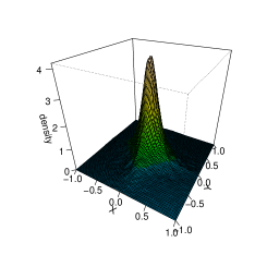
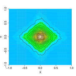
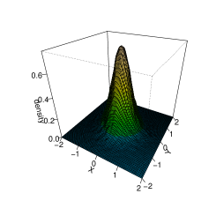
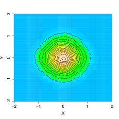
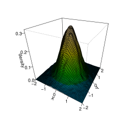
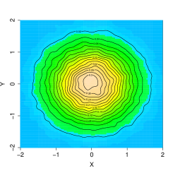
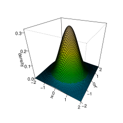
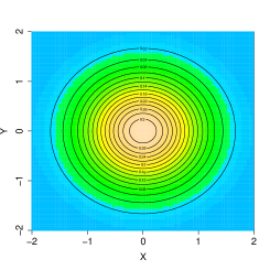
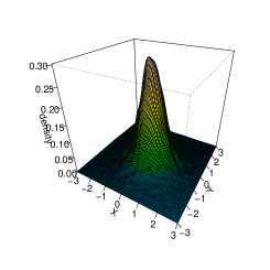
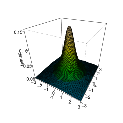
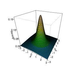
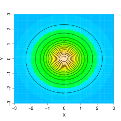
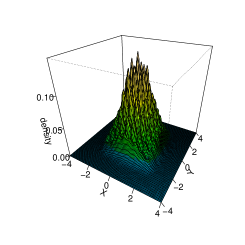
Figure 1: Gaussian target; statistics of $100000$ random paths: surrogate pdf evolution and its OXY projection for a) $t=0.2$, b) $t=0.7$, c) $t=15$. The subfigure d) refers to the asymptotic pdf (14). All trajectories were started form the origin $(0,0)$.

II Gillespie’s algorithm: Fine tuning in 2D.

The Gillespie’s algorithm has been originally constructed to give a dynamical picture of a finite chain of chemical reactions, gillespie ; gillespie1 . There, switches between different chemical reaction channels can be re-interpreted as jumps between points in a finite state space. Since the number of allowed chemical channels is finite, a serious modification of an original algorithm must be created to account for very large (virtually infinite) state space we need to consider in connection with Lévy flights. As an example, a jump process analog of chemical reaction channels could comprise (take $R^{1}$ for a while) all jumps form a fixed point $x_{0}$ to any point in the set $[x_{0}-\epsilon_{2},x_{0}-\epsilon_{1}]\cup[x_{0}+\epsilon_{1},x_{0}+\epsilon_{2}]$. Since we aim at numerical simulations, it is obvious that all admissible jumps cannot be computer-generated. Therefore, we must restrict considerations to a large number of suitably selected ”representative” jumps of a truncated jump process ruled by the truncated Lévy distribution of jumps.

Basic tenets of the modified Gillespie’s algorithm, fine tuned to account for Lévy jumps in $R^{1}$ have been described in detail elsewhere, zaba . Presently, we shall give a brief outline of the algorithm that is capable to account for Lévy flights in $R^{2}$. We mimic previously devised 1D steps, zaba , while adopting them to the 2D situation.

Eq. (7) can be rewritten as follows

$$\partial_{t}\rho(x,y)=\iint\limits_{A^{\prime}}C_{\mu}[w_{\phi}(x,y|\xi+x,\eta+y)\rho(\xi+x,\eta+y)-w_{\phi}(\xi+x,\eta+y|x,y)\rho(x,y)]d\xi\,d\eta,$$ (10)

where

$$\begin{split}&A^{\prime}=\{(\xi,\eta)\in\mathbb{R}^{2};\quad{\varepsilon_{1}^{x}\leqslant|\xi|\leqslant\varepsilon_{2}^{x}}\,\wedge\,{\varepsilon_{1}^{y}\leqslant|\eta|\leqslant\varepsilon_{2}^{y}}\},\\ &C_{\mu}=\frac{2^{\mu}\sin(\pi\mu/2)[\Gamma((\mu+2)/2)]^{2}}{\pi^{2}(\xi^{2}+\eta^{2})^{(\mu+2)/2}},\end{split}$$ (11)

The algorithm outline reads as follows:
(i) Set time $t=0$ and the point of origin for jumps, $(x_{0},y_{0})\in R^{2}$.
(ii) Create the set of all admissible jumps from $(x_{0},y_{0})$ to $(x_{0}+\xi,y_{0}+\eta)$, compatible with the transition rate $w_{\phi}(x,y|x+\xi,y+\eta)$.
(iii) Evaluate

$$\begin{split}&W_{1}(x_{0},y_{0})=\int\limits_{-\varepsilon_{2}^{x}}^{-\varepsilon_{1}^{x}}\int\limits_{-\varepsilon_{2}^{y}}^{-\varepsilon_{1}^{y}}C_{\mu}w_{\phi}(\xi+x_{0},\eta+y_{0}|x_{0},y_{0})d\xi\,d\eta,\quad W_{2}(x_{0},y_{0})=\int\limits_{-\varepsilon_{2}^{x}}^{-\varepsilon_{1}^{x}}\int\limits_{\varepsilon_{1}^{y}}^{\varepsilon_{2}^{y}}C_{\mu}w_{\phi}(\xi+x_{0},\eta+y_{0}|x_{0},y_{0})d\xi\,d\eta,\\ &W_{3}(x_{0},y_{0})=\int\limits_{\varepsilon_{1}^{x}}^{\varepsilon_{2}^{x}}\int\limits_{-\varepsilon_{2}^{y}}^{-\varepsilon_{1}^{y}}C_{\mu}w_{\phi}(\xi+x_{0},\eta+y_{0}|x_{0},y_{0})d\xi\,d\eta,\quad W_{4}(x_{0},y_{0})=\int\limits_{\varepsilon_{1}^{x}}^{\varepsilon_{2}^{x}}\int\limits_{\varepsilon_{1}^{y}}^{\varepsilon_{2}^{y}}C_{\mu}w_{\phi}(\xi+x_{0},\eta+y_{0}|x_{0},y_{0})d\xi\,d\eta,\end{split}$$ (12)

and $W(x_{0},y_{0})=W_{1}(x_{0},y_{0})+W_{2}(x_{0},y_{0})+W_{3}(x_{0},y_{0})+W_{4}(x_{0},y_{0})$.
(iv) Using a random number generator draw $p_{x},p_{y}\in[0,1]$ from a uniform distribution
(v) Employing above $p_{x}$ and $p_{y}$ and the identities

$$\left\{\begin{array}[]{ll}\int\limits_{-\varepsilon_{2}^{x}}^{b_{x}}\left(\int\limits_{-\varepsilon_{2}^{y}}^{-\varepsilon_{1}^{y}}C_{\mu}w_{\phi}(\xi+x_{0},\eta+y_{0}|x_{0},y_{0})d\eta+\int\limits_{\varepsilon_{1}^{y}}^{\varepsilon_{2}^{y}}C_{\mu}w_{\phi}(\xi+x_{0},\eta+y_{0}|x_{0},y_{0})d\eta\right)d\xi=p_{x}W(x_{0},y_{0}),&\hbox{$p_{x}<W_{12}(x_{0},y_{0})/W(x_{0},y_{0})$;}\\ W_{12}(x_{0},y_{0})+\int\limits_{\varepsilon_{1}^{x}}^{b_{x}}\left(\int\limits_{-\varepsilon_{2}^{y}}^{-\varepsilon_{1}^{y}}C_{\mu}w_{\phi}(\xi+x_{0},\eta+y_{0}|x_{0},y_{0})d\eta+\int\limits_{\varepsilon_{1}^{y}}^{\varepsilon_{2}^{y}}C_{\mu}w_{\phi}(\xi+x_{0},\eta+y_{0}|x_{0},y_{0})d\eta\right)d\xi=p_{x}W(x_{0},y_{0}),&\hbox{$p_{x}\geqslant W_{12}(x_{0},y_{0})/W(x_{0},y_{0})$;}\\ \int\limits_{-\varepsilon_{2}^{y}}^{b_{y}}\left(\int\limits_{-\varepsilon_{2}^{x}}^{-\varepsilon_{1}^{x}}C_{\mu}w_{\phi}(\xi+x_{0},\eta+y_{0}|x_{0},y_{0})d\xi+\int\limits_{\varepsilon_{1}^{x}}^{\varepsilon_{2}^{x}}C_{\mu}w_{\phi}(\xi+x_{0},\eta+y_{0}|x_{0},y_{0})d\xi\right)d\eta=p_{y}W(x_{0},y_{0}),&\hbox{$p_{y}<W_{13}(x_{0},y_{0})/W(x_{0},y_{0})$;}\\ W_{13}(x_{0},y_{0})+\int\limits_{\varepsilon_{1}^{y}}^{b_{y}}\left(\int\limits_{-\varepsilon_{2}^{x}}^{-\varepsilon_{1}^{x}}C_{\mu}w_{\phi}(\xi+x_{0},\eta+y_{0}|x_{0},y_{0})d\xi+\int\limits_{\varepsilon_{1}^{x}}^{\varepsilon_{2}^{x}}C_{\mu}w_{\phi}(\xi+x_{0},\eta+y_{0}|x_{0},y_{0})d\xi\right)d\eta=p_{y}W(x_{0},y_{0}),&\hbox{$p_{y}\geqslant W_{13}(x_{0},y_{0})/W(x_{0},y_{0})$,}\end{array}\right.$$ (13)

where $W_{12}(x_{0},y_{0})=W_{1}(x_{0},y_{0})+W_{2}(x_{0},y_{0})$ i $W_{13}(x_{0},y_{0})=W_{1}(x_{0},y_{0})+W_{3}(x_{0},y_{0})$, find $b_{x}$ and $b_{y}$ corresponding to the ”transition channel” $(x_{0},y_{0})\rightarrow(b_{x},b_{y})$ .
(vi) Draw a new number $q\in(0,1)$ from a uniform distribution.
(vii) Reset time label s $t=t+\Delta t$ where : $\Delta t=-\ln q/W(x_{0},y_{0})$.
(viii) Reset $(x_{0},y_{0})$ to a new location $(x_{0}\doteq x_{0}+b_{x},y_{0}\doteq y_{0}+b_{y})$, considered as a reference point for the iterative procedure.
(ix) Return to step (ii) and repeat the procedure anew.

Remark: All precautions respected in 1D need to be respected in 2D as well (c.f. Comment 1 in zaba ). The following jump size bounds (integration boundaries) were adopted for exemplary numerical procedures to be described in below: $\varepsilon_{1}^{x}=\varepsilon_{1}^{y}=\varepsilon_{1}=0.001$ i $\varepsilon_{2}^{x}=\varepsilon_{2}^{y}=\varepsilon_{2}=1$, provided one keeps in memory our convention not to reproduce the $x,y$ index in $\varepsilon_{1,2}^{x,y}$ anymore.

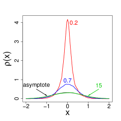
Figure 2: $y=0$ projection of the previous pdf data ($100000$ trajectories) for running time instants a) $t=0.2$, b) $t=0.7$, c) $t=15$, d) a projection of the target pdf is depicted.

a)

b)

Figure 3: Time evolution of a) the first moment (average $r=\sqrt{x^{2}+y^{2}}$ value) , b) second moment (mean value of $r^{2}$). All $100000$ trajectories originate from $(0,0)$.

III Statistics of random paths in 2D: Case studies of the pdf evolution.

Our main purpose in the present section is to analyze the response of free Lévy noise to generic external potentials. That has been previously found to be encoded in jump transition rates. Now we address the same problem in a path-wise fashion. We shall faithfully follow the outlined random path generation procedure. Once suitable path ensemble data are collected, we shall verify whether statistical (ensemble) features of generated random trajectories are compatible with those predicted by the master equation (7). This includes a control of an asymptotic behavior $\rho(x,t)\to\rho_{*}(x)$ with $x\in R^{2}$, when $t\to\infty$.

III.1 Harmonic confinement: Gaussian target

Let us prescribe an asymptotic invariant pdf $\rho_{*}$ to be in a 2D Gaussian form:

$$\rho_{*}(x,y)=\frac{1}{\pi}e^{-x^{2}-y^{2}}.$$ (14)

As an exemplary source of random noise we assume the Cauchy driver, i.e. 2D Lévy-stable noise with the stability index $\mu=1$. Accordingly, the jump transition rate reads:

$$C_{1}\,w_{\phi}(\xi+x,\eta+y|x,y)=\frac{1}{2\pi}\frac{e^{-\xi^{2}/2-x\xi-\eta^{2}-y\eta}}{(\xi^{2}+\eta^{2})^{3/2}}.$$ (15)

To generate sample paths of the process, we need first to evaluate integrals of (15) over suitable integration volumes. If the integration volume comprises $x,y$ which are close to the jump size boundaries $\pm\varepsilon_{1}$, one develops a numerator of an expression into Taylor series and keeps terms up to the quadratic one. Errors induced by such approximation procedure are marginal. On the other hand, if $x,y$ are far away from $\pm\varepsilon_{1}$ integrals (15) are amenable to standard evaluation methods (like e.g. Simposon’s one). To be more explicit in this respect, let $\varepsilon_{12}=0.05$. If $|a|,|b|,|c|,|d|\leqslant\varepsilon_{12}$, then

$$\int\limits_{a}^{b}\int\limits_{c}^{d}\frac{e^{-\xi^{2}/2-x\xi-\eta^{2}-y\eta}}{(\xi^{2}+\eta^{2})^{3/2}}d\xi\,d\eta\thickapprox\int\limits_{a}^{b}\int\limits_{c}^{d}\frac{(1-x\xi+\frac{x^{2}-1}{2}\xi^{2})(1-y\eta+\frac{y^{2}-1}{2}\eta^{2})}{(\xi^{2}+\eta^{2})^{3/2}}d\xi\,d\eta\thickapprox\sum\limits_{i=1}^{6}\mathbb{I}_{i},$$ (16)

where

$$\begin{split}&\mathbb{I}_{1}=\int\limits_{a}^{b}\int\limits_{c}^{d}\frac{d\xi\,d\eta}{(\xi^{2}+\eta^{2})^{3/2}}=\int\limits_{a}^{b}\left(\frac{d}{\xi^{2}\sqrt{\xi^{2}+d^{2}}}-\frac{c}{\xi^{2}\sqrt{\xi^{2}+c^{2}}}\right)d\xi=-\frac{\sqrt{b^{2}+d^{2}}}{bd}+\frac{\sqrt{a^{2}+d^{2}}}{ad}+\frac{\sqrt{b^{2}+c^{2}}}{bc}-\frac{\sqrt{a^{2}+c^{2}}}{ac},\\ &\mathbb{I}_{2}=-\int\limits_{a}^{b}\int\limits_{c}^{d}\frac{x\xi d\xi\,d\eta}{(\xi^{2}+\eta^{2})^{3/2}}=x\ln\left(\frac{(d+\sqrt{b^{2}+d^{2}})(c+\sqrt{a^{2}+c^{2}})}{(c+\sqrt{b^{2}+c^{2}})(d+\sqrt{a^{2}+d^{2}})}\right),\\ &\mathbb{I}_{3}=-\int\limits_{a}^{b}\int\limits_{c}^{d}\frac{y\eta d\xi\,d\eta}{(\xi^{2}+\eta^{2})^{3/2}}=y\ln\left(\frac{(b+\sqrt{b^{2}+d^{2}})(a+\sqrt{a^{2}+c^{2}})}{(a+\sqrt{a^{2}+d^{2}})(b+\sqrt{b^{2}+c^{2}})}\right),\\ &\mathbb{I}_{4}=\int\limits_{a}^{b}\int\limits_{c}^{d}\frac{xy\xi\eta d\xi\,d\eta}{(\xi^{2}+\eta^{2})^{3/2}}=xy(\sqrt{a^{2}+d^{2}}+\sqrt{b^{2}+c^{2}}-\sqrt{b^{2}+d^{2}}-\sqrt{a^{2}+c^{2}}),\\ &\mathbb{I}_{5}=\int\limits_{a}^{b}\int\limits_{c}^{d}\frac{x^{2}-1}{2}\frac{\xi^{2}d\xi\,d\eta}{(\xi^{2}+\eta^{2})^{3/2}}=\frac{x^{2}-1}{2}\left(d\ln\left(\frac{b+\sqrt{b^{2}+d^{2}}}{a+\sqrt{a^{2}+d^{2}}}\right)-c\ln\left(\frac{b+\sqrt{b^{2}+c^{2}}}{a+\sqrt{a^{2}+c^{2}}}\right)\right),\\ &\mathbb{I}_{6}=\int\limits_{a}^{b}\int\limits_{c}^{d}\frac{y^{2}-1}{2}\frac{\eta^{2}d\xi\,d\eta}{(\xi^{2}+\eta^{2})^{3/2}}=\frac{y^{2}-1}{2}\left(b\ln\left(\frac{d+\sqrt{b^{2}+d^{2}}}{c+\sqrt{b^{2}+c^{2}}}\right)-a\ln\left(\frac{d+\sqrt{a^{2}+d^{2}}}{c+\sqrt{a^{2}+c^{2}}}\right)\right).\end{split}$$ (17)

Numerical routines were written in terms of C-codes, available .

In Fig. 1 we have depicted the statistical data inferred from 100 000 trajectories, for three running time instants $t=0.2$, $t=0.7$, $t=15$, together with the asymptotic expression (14). The right-hand-side column depicts projections of those data upon the the $OXY$ plane. A substanitial increase of the analyzed enesemble data (like e.g. $300000$, $500000$ or $10^{6}$) is merely a matter of the simulation time span and adds nothing inspiring to the obtained behavior.

Figure 4: Cauchy target; surrogate pdf evolution inferred from $100000$ sample trajectories and the OXY projection for running times a) $t=0.2$, b) $t=3$, c) $t=500$. A subfigure d) refers to the target Cauchy pdf 19). In the course of simulations all trajectories were started from $(0,0)$.

It is clear that the surrogate pdf evolution consistently goes towards an invariant asymptotic pdf (compare subfigures c) and d)). We note a lowering and flattening of the maximum around $(0,0)$, in consistency with the ultimate target outcome, whose height is $1/\pi$ as follows from $\rho_{*}(0,0)=1/\pi$. Visually accessible in homogeneities of circular shapes in OXY projections b) i c), are a consequence of still relatively low number (100 000) of sample paths data and approximations involved in evaluating involved integrals. The shape of OXY projection a) is a consequence of the initial data choice. Our problem has a radial symmetry. Therefore in Fig. 2 we depict a projection of the trajectory induced data upon the $y=0$ plane. The projection shows as well a consistent convergence towards the target pdf.

An additional control method for the path-wise inferred pdf evolution, addresses the time evolution and an asymptotic behavior of the pdf moments $<R(t)>$ and $<R^{2}(t)>$. Here $<R(t)>$ is the mean distance of $(x,y)$ points of a trajectory form the origin $(0,0)$ at the running time instant $t$, while $<R^{2}(t)>$ is a mean square distance from $(0,0)$. In view of

$$\begin{split}<R>_{as}=\frac{1}{\pi}\iint\limits_{\mathbb{R}^{2}}\sqrt{x^{2}+y^{2}}e^{-x^{2}-y^{2}}=\frac{\sqrt{\pi}}{2}\thickapprox 0.886,\\ <R^{2}>_{as}=\frac{1}{\pi}\iint\limits_{\mathbb{R}^{2}}(x^{2}+y^{2})e^{-x^{2}-y^{2}}=1,\end{split}$$ (18)

the $<R(t)>$ dynamics should set down at $\sqrt{\pi}/2$, while this of $<R^{2}(t)>$ at $1$. Fig. 3 depicts the evolution of $<R(t)>$ and $<R^{2}(t)>$, inferred from the simulated sample of $100000$ jumping paths.

The observed convergence $<R(t)>\rightarrow 1/\pi$ and $<R^{2}(t)>\rightarrow 1$ validates the number generator choice, we have used to arrive at sample jumping paths.

Figure 5: The projection of the previous pdf data on the $y=0$ plane, at time instants a) $t=0.2$, b) $t=3$, c) $t=500$, d) target pdf projection.

III.2 Logarithmic confinement: 2D Cauchy target.

We consider the target pdf $\rho_{*}$ in the 2D Cauchy form:

$$\rho_{*}(x,y)=\frac{1}{2\pi}\frac{1}{(1+x^{2}+y^{2})^{3/2}}.$$ (19)

Like previously, we take the Cauchy driver, $\mu=1$, as a reference Lévy stable noise. Accordingly:

$$C_{1}w_{\phi}(\xi+x,\eta+y|x,y)=\frac{1}{2\pi}\frac{1}{(\xi^{2}+\eta^{2})^{3/2}}\left(\frac{1+x^{2}+y^{2}}{1+(x+\xi)^{2}+(y+\eta)^{2}}\right)^{3/4}.$$ (20)

Proceeding like in the Gaussian case, for small $\xi$ and $\eta$, Eq. (20) can be approximated by

$$\frac{1}{2\pi}\frac{1}{(\xi^{2}+\eta^{2})^{3/2}}\left(1-\frac{3x}{2(1+x^{2}+y^{2})}\,\xi-\frac{3y}{2(1+x^{2}+y^{2})}\,\eta\right),$$ (21)

where terms linear in $\xi$ i $\eta$ were preserved. The result can be analytically integrated term after term by employing Eqs. (17)..

Accumulated trajectory data have been analyzed to produce Fig. 4, where a surrogate pdf evolution is displayed. Fig. 5 reproduces the $y=0$ projection of the obtained pdf data. If compared with the 1D case analyzed in Ref. zaba a convergence to Boltzmannian equilibrium (target pdf) is substantially slowed down.

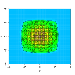
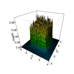
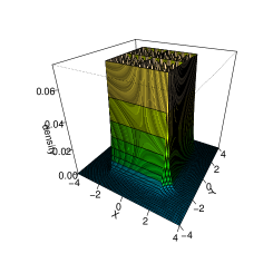
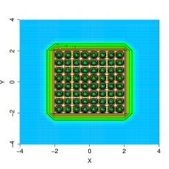
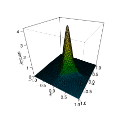
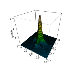
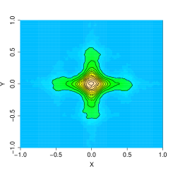
Figure 6: Locally periodic target; surrogate pdf evolution and its OXY projection inferred from $100000$ trajectories at running time instants a) $t=0.2$, b) $t=3$, c) $t=300$. The subfigure d) depicts the asymptotic pdf (22). All trajectories have been started from $(0,0)$.

III.3 Locally periodic confinement in $R^{2}$.

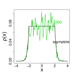
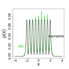
Figure 7: Projections of the surrogate pdf data at $t=300$ upon planes a) $y=0$, b) $y=1/4$, c) $y=x$. An ”asymptote” refers to the target pdf projections

We consider target pdf whose Boltzmanian exponent is locally periodic (within a finite rectangle) and almost entirely localized within a finite spatial area due to harmonically confining tails of the potential:

$$\rho_{*}(x,y)=\frac{1}{C}\left\{\begin{array}[]{ll}e^{-3\sin^{2}(2\pi x)\sin^{2}(2\pi y)},&\hbox{$|x|\leqslant 2$ i $|y|\leqslant 2$;}\\ e^{-x^{2}-y^{2}+8},&\hbox{$|x|>2$ i $|y|>2$;}\\ e^{-x^{2}+4},&\hbox{$|x|>2$ i $|y|\leqslant 2$;}\\ e^{-y^{2}+4},&\hbox{$|x|\leqslant 2$ i $|y|>2$,}\end{array}\right.$$ (22)

The normalization constant $C$ actually reads $C=13.5921$.

Subsequently adopted numerical integration routines heavily rely on the experience gained during our previous case studies. In Fig. 6 we report the surrogate pdf evolution, inferred from $100000$ sample trajectories. A convergence rate to the asymptotic (target) pdf is satisfactory, although a reasonable agreement with the target data has been achieved for relatively large running time values, here $t=300$.

We are aware of the fact that the number of $100000$ trajectories may be considered as too small and not sufficiently representative sample. Our tentative $300000$ paths data do not show significant qualitative changes in the obtained evolution picture.

We should mention that there are significant statistical fluctuations to be kept under control. They become are very conspicuous if the number of involved trajectories gets significantly lowered by imposing constraints (like e.g. various spatial projections). All l trajectory data, after being gathered, are safely stored in the computer memory. Therefore we can get access to any conceivable and more detailed statistical picture of what is going on, even if the outcome is hampered by significant random deviations from the reference (target) pdf data..

A sample of such fluctuating data is provided in Fig. 7, where we have considered projections of the surrogate pdf data upon planes $y=0$, $y=1/4$ and $y=x$ at time $t=300$. We have set them in a direct comparison with respective target pdf (12) data.

IV Outlook

We have taken into consideration jump-type processes which can not be handled by standard stochastic differential equation methods (e.g. the Langevin modeling, where a conspicuous motion ”tendency” quantified by an additive drift term, can be unambiguously isolated from the noise contribution). Existing popular algorithms cannot provide a direct numerical simulation of sample paths of such non-standard processes. In the present paper, we have proposed a working method to generate stochastic trajectories (sample paths) of a random jump-type process that avoids any reference to a stochastic differential equation. An additional gain of that procedure is that we are in fact capable of reliably approximating the time evolution $\rho(x,t)$ of a true (typically not available in a closed analytic form) solution of the master equation.

To this end we have modified the Gillespie algorithm, gillespie ; gillespie1 , normally devised for sample paths generation if the transition rates refer to a finite number of states of a system. The essence of our modification is that we take into account the continuum of possible transition rates, thereby changing the finite sums in the original Gillespie algorithm into integrals. The corresponding procedures for stochastic trajectories generation have been changed accordingly.

In other words, here we are able (i) to extract the background sample paths of a jump process and (ii) to infer a reliable approximation of an actual (analytically unavailable) solution of the master equation (7)- (8). We emphasize once more here, that we have focused on those jump-type processes that cannot be modeled by any stochastic differential equation of the Langevin type.

Although heavy-tailed Lévy stable drivers were involved in the present considerations, we have clearly confirmed that a large variety of stationary target distributions is dynamically accessible for each particular $\mu\in(0,2)$ Lévy driver choice. That variety comprises not only the standard Gaussian pdf, casually discussed in relation to the Brownian motion (e.g. the Wiener process), but the whole non-Gaussian family, associated with the Lévy stable conceptual imagery .

Among heavy-tailed distributions, we have paid attention to the Cauchy pdf which can stand for an asymptotic target for any $\mu\in(0,2)$ driver, provided a steering environment (e.g. ”potential landscape”) is properly devised. In turn, the Cauchy driver, while excited in a proper environment, may lead to an asymptotic pdf with an arbitrarily large number of moments, the previously mentioned Gaussian case being included. . An example of the locally periodic environment has been considered as a toy model for more realistic physical systems. Our major hunch are strongly inhomogeneous ”potential landscapes”, modeled by relatively smooth potentials. We note that a radically extreme variant could be random potentials of Ref. geisel .

In connection with the master equation which was our departure point let us stress that, even if various mean field data are available in experimentally realizable systems, it is of vital interest to gain some knowledge about the microscopic dynamics (random paths) realized by the random system under consideration. The detailed analysis of sample path data with a focus on their specific features like e.g. ergodicity, mixing or lack of those properties, deserves a separate analysis. These goals can be achieved as well within the present simulation framework. It suffices to re-analyze the path-wise data we have collected and stored in the trajectory generation process.

References

• (1) H. Risken, The Fokker-Plack Equation, (Springer-Verlag, Berlin, 1989)
• (2) S. Jespersen, R. Metzler and H. C. Fogedby, Phys. Rev. E59, 2736, (1999)
• (3) I. Eliazar and J. Klafter, J. Stat. Phys. 119, 165, (2005)
• (4) P. Garbaczewski and R. Olkiewicz, J. Math. Phys. 40, 1057, (1999)
• (5) P. Garbaczewski and V. A. Stephanovich, Phys. Rev. E 80, 031113, (2009)
• (6) D. Brockmann and I. M. Sokolov, Chemical Physics, 284, 409, (2002)
• (7) D. Brockmann and T. Geisel, Phys. Rev. Lett. 90, 170601, (2003)
• (8) V. V. Belik and D. Brockmann, New. J. Phys. 9, 54, (2007)
• (9) P. Garbaczewski and V. A. Stephanovich, Physica A 389, 4410, (2010)
• (10) P. Garbaczewski and V. Stephanovich, Phys. Rev. E 84, 011142 (2011)
• (11) T. D. Gillespie, J. Phys. Chemistry, 8 (25), 2340, (1977)
• (12) T. D. Gillespie, J. Comput. Physics, 22 (4), 403, (1976)
• (13) M. Żaba, P. Garbaczewski and V. Stephanovich, Lévy flights in confining environments: Random paths and their statistics, arXiv: 1209.5882
• (14) C-codes available upon request