Partially supported by Spanish grants with Feder funds P09-FQM-4496 (J. Andalucía) and MTM2010–18099 (Mineco).
On the completeness of trajectories for some mechanical systems
Abstract
The classical tools which ensure the completeness of both, vector fields and second order differential equations for mechanical systems, are revisited. Possible extensions in three directions are discussed: infinite dimensional Banach (and Hilbert) manifolds, Finsler metrics and pseudo-Riemannian spaces, the latter including links with some relativistic spacetimes. Special emphasis is taken in the cleaning up of known techniques, the statement of open questions and the exploration of prospective frameworks.
1 Introduction
As explained in the classical Abraham & Marsden book (AM, , p. 71), the completeness of vector fields is often stressed in the literature since it corresponds to well-defined dynamics persisting eternally. However, in many circumstances one has to live with incompleteness and, in this case, incompleteness may mean the failure of our model. Remarkably, this happens in General Relativity, where singularities have become so common (Schwarzschild spacetime, Raychauduri equation, theorems by Penrose and Hawking…) that one expects to find incompleteness under physically reasonable general assumptions —and one hopes that the quantum viewpoint will be able to explain the physical meaning of singularities. In any case, the possible completeness or incompleteness becomes a fundamental property of the model.
In his early works at the beginning of the seventies, Marsden gave two remarkable results on completeness. The first, in collaboration with Weinstein WM , extends previous works on the completeness of Hamiltonian vector fields by Gordon Go , Ebin Eb and others. The second, about the geodesic completeness of compact homogeneous pseudo-Riemannian manifolds MaHomog , was one of the few results ensuring completeness instead of incompleteness in the Lorentzian setting of that time. The results on the side of geodesics in the Lorentzian setting have increased notably since then (see the review CS ). Moreover, some connections with the original Riemannian results for Hamiltonian systems have appeared. This has been a stimulus for the recent update and extension of such Riemannian results carried out by the author and his coworkers in CRS .
The aim of this paper is to revisit these results, formulating them in a general framework, and pointing out new open questions as well as new lines of study. The paper is organized into three parts. In the first (Section 2), some preliminaries on infinite-dimensional Banach manifolds endowed with Finsler metrics are introduced. From our viewpoint, this is the natural framework for the completeness of first order systems (vector fields), and some second order ones can be reduced to this setting.
In Section 3 we study completeness for both, first and second order systems. For first order, we review some old results Go ; Eb ; WM ; AM ; AMR formulating them in the general Banach Finsler case, and also allowing the time-dependence of the vector fields. We introduce primary bounds (Definition 1) here, which allow the purification of previous techniques (Theorem 3.1). For second order, i.e., trajectories accelerated by potentials and other time-dependent forces, we give a general result on completeness in Riemannian Hilbert manifolds (Theorem 3.2), which summarizes and extends those in Go ; Eb ; WM ; CRS . The latter are also simplified technically because, even though our proof uses comparison criteria between differential equations as in previous references, here such criteria are reduced essentially to the elementary lemma 1 —and the bounds through positively complete functions introduced in WM reduce to primary bounds as well. We suggest the possibility of going further in two directions: the time-dependence of the potentials and the Finsler Banach framework.
Section 4 deals with (finite-dimensional) pseudo-Riemannian manifolds. Here there is a great diversity of results and techniques (see CS ), and we focus on two topics. Firstly, results regarding manifolds with a high degree of symmetry. In particular, the extension of Marsden’s Theorem 4.3 to conformally related metrics (Theorem 4.4), is explained by using the techniques in the previous section. Secondly, the geometry of wave type spacetimes. This provides a simple link between Riemannian and Lorentzian results (Theorem 4.7) with new exciting open questions —some of them collected together at the end.
2 Preliminaries on infinite-dimensional manifolds
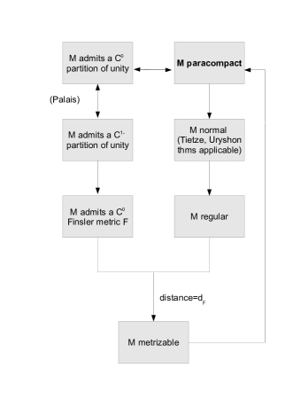
Some preliminaries on Banach manifolds are introduced here. Results on the elements which will be relevant for the posterior results will be gathered together, and a framework for tentative generalizations will be provided. Special emphasis is focused on the role of paracompactness for the ambient manifold, as this condition will be equivalent to the existence of a -Finsler metric such that its associated distance metrizes the manifold topology. The role of smoothability for Finsler metrics is also emphasized. Essentially, smoothability is sufficient for distance estimates in first order problems (Section 3.1), but further smoothability may be required for the development of second order ones (Section 3.2).
We will follow conventions on Banach and Hilbert manifolds as in the original papers by Palais PalaisProcSym_CriticalPointTh68 ; PalaisTop_LustSch66 ; PalaisTop_Hilbert63 , as well as books such as Abraham, Marsden & Ratiu AMR , Lang Lang , Deimling De , Kriegl & Michor Michor or Moore’s notes Moore .
Topological conventions on Banach manifolds. Any Banach manifold will be always assumed with , as well as connected, Hausdorff and paracompact and, thus, normal111In particular, our Banach manifolds will be always regular and, so, some difficulties pointed out by Palais in PalaisProcSym_CriticalPointTh68 (see Sect. 2 including the Appendix therein), will not apply. The central role of paracompactness from the topological viewpoint is stressed in Figure 1. Notice that, as a difference with the finite dimensional case, second countability does not imply paracompactness (see for example MargalefOuterelo , (Michor, , Sect. 27.6) or PalaisProcSym_CriticalPointTh68 ).. A -manifold will be a finite dimensional Banach manifold with dimension . When the infinite dimension is allowed, we will remark explicitly that is Banach (say, modelled on some Banach space with norm ) or, when applicable, that it is Hilbert (modelled on some real Hilbert space with inner product ). When indefinite metrics are considered, as in Section 4, will be typically a -manifold.
Finsler Banach manifolds. will denote a (reversible) Finsler metric on the Banach manifold , and will be called a Finsler Banach manifold. This notion is taken in the sense of Palais PalaisTop_LustSch66 , that is, yields a norm at each tangent space:
| (1) |
which admits a chart such that the induced norms
| (2) |
(here denotes the differential or tangent map) satisfy: (a) they are equivalent to the natural norm of (i.e., for some and all ) , and (b) they vary continuously at (i.e., for each there exists a neighborhood of such that for all ).
As norms cannot be differentiable at222By the same reason that neither is the absolute value function on . Moreover, at least in the finite-dimensional case, the square of a norm is smooth at 0 if and only if the norm comes from a scalar product (Wa, , Prop. 4.1). 0, the differentiability of the norm means always away from . The Finsler metric is called (for ) if is and varies smoothly with in a way (i.e., for any chart as above the map is ).
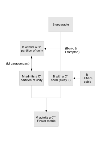
Existence of Finsler metrics. The question of the existence of a Finsler metric depends only on topological grounds, but the existence of a one with is much subtler. Namely, on the one hand the hypothesis of paracompactness on becomes equivalent to the existence of -partitions of the unity subordinated to any open covering. By a result of Palais (PalaisTop_LustSch66, , Th. 1.6), (PalaisProcSym_CriticalPointTh68, , Sect. 3), it is also equivalent to the existence of locally Lipschitz partitions of the unity, and this allows ensuring the existence of Finsler metrics in any Banach manifold (PalaisTop_LustSch66, , Th. 2.11). On the other hand, when the model Banach space admits partitions of the unity subordinate to any open covering (which happens, in particular, when is separable and admits a norm away from 0, see BF , (AMR, , Prop. 5.5.18, 5.5.19)), then the Banach manifold also admits partitions of the unity (AMR, , Th. 5.5.12) and, in this case, admits -Finsler metrics too (Figure 2).
Remark 1
It is worth pointing out that, even though the differentiability of may be useful for some issues (see Section 3.2 below), it will not be especially relevant for the estimates which involve length or distances in the first order problems to be studied in Section 3.1. This fact is used implicitly in time-dependent problems. In fact, this case is commonly handled by transforming it into a non time-dependent one, defined on the product manifold which is endowed with a natural direct sum of Finsler metrics (namely, the addition of the Finsler metrics of the factors), see Remark 3. Nevertheless, this direct sum is non-differentiable away from 0 even if differentiability is assumed for the metric on each factor (notice that it is not guaranteed the differentiability on a vector tangent to the product whenever one of its two components is equal to zero).
Associated distance. Remember that our definition of a Finsler metric includes its reversibility (i.e., for all tangent vector ). So, defines a natural distance by taking the infimum of the lengths of the curves connecting each pair of points. This distance will be denoted or, simply, if there is no possibility of confusion. One can prove that the topology generated by agrees with the manifold topology by using the regularity of the manifold. (PalaisProcSym_CriticalPointTh68, , p. 202) and, so, that all Finsler Banach manifolds are metrizable333Consistently, paracompactness can be deduced from the hypothesis of metrizability (or even just from pseudo-metrizability, see (AMR, , Lemma 5.515))..
We will speak about the completeness of in the sense of metric completeness, i.e., the convergence of Cauchy sequences for . One can also consider geodesics for (for example, in the sense of locally length-minimizing curves of constant speed, with other characterizations under further smoothability, see Section 3.2) and we will say that is geodesically complete when its inextensible geodesics are defined on all . In the infinite-dimensional case, the completeness of implies geodesic completeness but, as stressed by Atkin At , neither geodesic completeness implies metric completeness nor other consequences of Hopf-Rinow theorem hold.
In order to make estimates with the distances, we fix a base point and denote
| (3) |
(This notation will be used when the properties under study are independent of the chosen point ).
Pseudo-Riemannian metrics on Banach manifolds. When the model space of the Banach manifold is reflexive, it is natural to define a pseudo-Riemannian metric as a choice of a continuous symmetric bilinear form at each tangent space such that the associated “flat” map (to lower indexes in finite dimension) into the dual space given by
| (4) |
is a homeomorphism (if this condition on were not imposed, one would speak of a weak pseudo-Riemannian metric, and the reflexivity of would not be required). The set of all such bilinear forms can be identified via a chart around with an open subset of the set BL of all the continuous symmetric bilinear forms on . As BL is naturally a Banach space too, the pseudo-Riemannian metric can be regarded as a section of a fiber bundle on with fiber BL (see (Lang, , Ch VII.1)).
Riemannian metrics on Hilbert manifolds. When the pseudo-Riemannian metric is positive definite then we say that it is Riemannian. As we are assuming that is a homeomorphism, the model space is then Hilberteable. So, it will be denoted , and we will consider only Riemannian metrics on Hilbert manifolds. Notice that, for any Riemannian metric , one has an associated Finsler metric given by for all . So, the bounds required in the definition of continuity for in the Finslerian case (see (a) and (b) below formula (2)), hold here in terms of the norm associated to the inner product of . Moreover, this norm is always away from 0. Thus, any Hilbert manifold modelled on a separable space admits partitions of the unity and, then, a Riemannian metric. Riemannian metrics on Hilbert manifolds, as well as their geodesics, are extensively studied in the literature, see for example Lang or, for the separable case, Kl . A type of Hopf-Rinow theorem for separable Riemann Hilbert manifolds can be found in (Kl, , Th. 2.1.3) (including the “Notes” therein; recall also At ); some related remarkable properties can be seen in Ek .
Concluding remarks and conventions. For the convenience of the reader, a summary on the topological and smooth-related results commented above is provided in Figures 1 and 2. Basic detailed background can be found in PalaisTop_LustSch66 ; PalaisProcSym_CriticalPointTh68 and AMR . In what follows, all the objects will be smooth i.e. as differentiable as possible according to the discussion above. In the case of first order problems (Section 3.1), this will mean at least for any Banach manifold and for any vector field on . As emphasized in Remarks 1 and 3, Finsler metrics are required only at this stage. Further requirements of smoothability will be needed for the second order case (Section 3.2). In the (indefinite) finite-dimensional case (Section 4), the issues on smoothability are not especially relevant and, so, the reader may either track them or just assume smoothability.
3 Completeness of trajectories in a positive-definite infinite-dimensional setting
This section is divided into two subsections. The first one is devoted to the problem of the completeness of a vector field. We start by reviewing some results. These have essentially been known from the seventies Go ; Eb ; WM and explained in AM ; AMR . They are extended here to the () Finsler setting when possible (Propositions 1, 2). Then, the notion of primarily complete function is introduced (Definition 1). Primary bounds for a vector field allows us to give an optimal result on completeness in the Finsler Banach case, Theorem 3.1. The time-dependent case is specially discussed in Remark 3 and the last part of the subsection.
In the second subsection, our Theorem 3.2 (plus Remark 6) summarizes and extends the results on second order differential equations in Go ; Eb ; WM ; CRS . The proof is carried out in three conceptually independent steps. The first one is just a standard reduction to the first order case. The second one deals with technical bounds. This is carried out here just by using systematically the simple lemma 1. In the third step, the subtleties of the infinite dimensional case (first studied by Ebin Eb ), are stressed.
Further discussions are also provided in this second subsection. Firstly, the relation between the previous notion of primarily complete function and Weinstein-Marsden’s positive completeness, is analyzed. Secondly, we consider specifically the time-dependent case. Even though natural bounds are obtained for the growth of the potential in this case, we also explore some alternatives. Finally, we discuss the difficulties of the generalization when the Riemannian metrics are replaced by Finslerian ones, and we provide a simple example for the (standard) finite-dimensional Finsler case.
3.1 Complete vector fields on Finsler Banach manifolds
Elementary criteria
The properties of the (local) flow of a vector field and, in particular, the existence of a flow box around each point, can be found, for example, in (AMR, , p. 192ff), (Lang, , p. 84ff) or (Moore, , Sect. 1.10). We start with a well-known result (see for example (AMR, , Prop. 4.1.19)).
Proposition 1
Let be a vector field on a Banach manifold , and let (resp. ) be an integral curve of with . Then, can be extended beyond as an integral curve of if and only if there exists a sequence such that the sequence (resp. ) is convergent in .
Proof
The necessity of the condition is obvious. For its sufficiency, let be the limit of the sequence. The existence of a flow box of at ensures the existence of a neighborhood of and some such that the integral curves of at any are defined on . So, taking large so that the integral curve through will be defined on and will be extensible through .
Accordingly, we will say that an integral curve of defined on some interval of is complete if it can be extended as an integral curve of to all , and will be complete if so are its integral curves.
Remark 2
(i) This result follows in the infinite-dimensional case as well as in the finite-dimensional one. However, the application in the latter case is easier, as is then locally compact. For example, Proposition 1 yields directly that, if the support of is compact (in particular, if is compact and, thus, finite-dimensional) then is complete.
(ii) Analogously, one can prove that if a Banach manifold admits a -proper map (i.e. is compact for any compact ), then a vector field is complete whenever
| (5) |
for some and all . In fact, (5) implies a bound for the derivative of . If the domain of the integral curve were bounded, a bound for on would be obtained too. As is proper, the result would follow then from Proposition 1 (see (AM, , 2.1.20) or (AMR, , 4.1.21) for more details). Even though proper maps are well behaved in Banach manifolds (for example, they are closed maps PalaisProcAMS_WhenProperMapsAreClosed ) results as the previous one are used typically in the finite-dimensional case (putting, for example, on a complete Riemannian -manifold).
The following criterion on completeness for Finsler Banach manifolds holds as in the case of Riemann Hilbert ones or Banach spaces (compare with (AM, , Prop. 2.1.2) or (AMR, , Prop. 4.1.22)).
Proposition 2
Let be a complete Finsler Banach manifold and a vector field on . If is an integral curve of and is bounded on bounded subintervals of , then is complete.
Proof
Assume with no loss of generality that , let be the assumed bound and choose . The associated distance satisfies then:
So, is a Cauchy sequence, which becomes convergent to some limit by the completeness of . Then, Proposition 1 can be applied to .
Remark 3
(The time-dependent case.) The results in the previous two propositions can be extended to the case when is time-dependent, and defined for all the values of the time.
More precisely, consider the product manifold , let , be the natural projections, and denote by the natural coordinate on . We say that is a time-dependent vector field on if it is a smooth section of the pull-back bundle , whose base is and each fiber comes from a tangent space to . Such a vector field yields naturally a (time-independent) vector field on which satisfies both, is naturally identifiable to the natural projection of on and , for all .
To speak about the integral curves of makes a natural sense (see for example (Lang, , Ch. IV)) and becomes equivalent to consider the integral curves of ; in fact, will be an integral curve of if and only if is an integral curve of . So, Proposition 1 is extended directly to a time-dependent .
To extend Proposition 2, recall that, if is a Finsler Banach manifold, then admits a natural Finsler metric obtained as the direct sum of and the usual one on (see Remark 1). Clearly, will be complete if and only if so is . Moreover, the -length of the integral curve of is bounded on finite intervals if and only so is the -length of the integral curve of , as required.
Applications
Next, we will apply previous results to simple but general situations. But, previously, we consider the following technical elementary result for future referencing (see for example (Te, , Lemma 1.1)).
Lemma 1
Consider the equation
| (6) |
where is locally Lipschitz in its second variable, and let be a subsolution of the differential equation i.e.,
| (7) |
Then, for every solution of (6) such that we have
| (8) |
The same conclusion (8) holds if is only locally Lipschitzian and the inequality (7) occurs when is replaced by some local Lipschitz bound around each .
The proof follows just recalling that close to by the assumptions and, if there were a first point such that , then (or an analogous inequality involving a local Lipschitz bound) holds, a contradiction.
Estimates of the growth for completeness. Let us introduce some auxiliary definitions.
Definition 1
A (locally Lipschitz) function is primarily complete if it is positive, non-decreasing and satisfies:
| (9) |
A vector field on a Finsler Banach manifold is primarily bounded if there exists a primarily complete function , which be called a bounding function, such that
| (10) |
In particular, grows at most linearly if it is primarily bounded by an affine bounding function, i.e.:
| (11) |
for some constants .
Remark 4
The best polynomial candidate for the bounding function has degree one as, clearly, no polynomial of higher degree can be a primarily complete function. Nevertheless, a slightly faster growth is allowed for non-polynomial functions. For example, will be primarily complete if it grows as for large (see also the discussion in the last part of Section 3.2).
Now, we can give a general bound for the completeness of vector fields.
Theorem 3.1
Any primarily bounded vector field on a complete Finsler Banach manifold is complete.
Proof
Let be an integral curve of . With no loss of generality, assume , , and choose in the notation introduced in (3). Then:
| (12) |
where is the bounding function. Thus, putting we can assume:
(or the analogous inequality for local Lipschitz constants). The unique inextensible solution of the equality
is defined for all , as its inverse is determined as and (9) holds. So, from lemma 1 one has
As is non-decreasing, equation (10) yields the bound so that Proposition 2 is applicable.
Remark 5
By considering on a vector field type one can check the optimality of Theorem 3.1 and, in particular, the optimality (in the sense discussed in Remark 4) of the at most linear growth of to ensure completeness. Of course, a vector field with a superlinear growth such as may be complete. In fact, in order to ensure completeness, only the growth of along the direction of its integral curves becomes relevant. This underlies in the fact that the sum of two complete vector fields may be incomplete (put and as before) and may suggest more refined hypotheses for completeness in Hilbert spaces (compare with (AMR, , Exercise 2.2H)).
Time-dependent case. As in the case of the criterions on completeness, Theorem 3.1 can be extended to the case of a time-dependent vector field . In fact, the proof works in a completely analogous way (with the observations in Remark 3), if the inequality in (9) is regarded as for all Nevertheless, one can be a bit more accurate.
Definition 2
A time-dependent vector field on a Finsler Banach manifold is primarily bounded along finite times if there exists a primarily complete function and a continuous function such that
In particular, grows at most linearly along finite times when can be chosen affine or, equivalently, when
| (13) |
for some functions
Corollary 1
Let be a time-dependent vector field on a complete Finsler Banach . If is primarily bounded along finite times then it is complete.
3.2 Completeness for 2nd order trajectories
General result on Riemann Hilbert manifolds
The next result, stated on a Riemann Hilbert manifold , will summarize those in Go ; Eb ; AM ; CRS . To state it, recall that the notion of time-dependent vector field on in Remark 3 can be directly translated to (continuous, linear) endomorphism fields, which will be regarded here as sections of a fiber bundle on with fiber at each equal to the vector space of bounded linear operators which vanish on . Given such a field , we will decompose it as where denotes its self-adjoint part , and the skew-adjoint one. A time-dependent or non-autonomous potential means just a smooth map , then, the notation makes a natural sense, and denotes the time dependent vector field on obtained by taking the gradient of at each slice constant with respect to , i.e., for . The pointwise norm induced by in any space of tensor fields will be denoted .
Theorem 3.2
Let be a complete Riemann Hilbert manifold, and consider a endomorphism field , a vector field and a potential on , all of them time–dependent and smooth. Assume that:
- (i)
-
is uniformly bounded along finite times, i.e., for all ,
- (ii)
-
grows at most linearly along finite times, i.e., for all , and
- (iii)
-
both, and grow at most quadratically along finite times, i.e., they are bounded by ,
where , denote positive functions. Then, the inextensible solutions of
| (14) |
are complete.
Proof
In order to clarify the ideas, the proof is divided into three steps.
Step 1: Reduce the problem to the completeness of a vector field on the tangent bundle. The second order equation (14) allows to define a vector field on the manifold such that each solution of (14) generates an integral curve of . This is standard (see for example (AM, , Ch. 3) or, for explicit details on the time-dependent case, (CRS, , Section 3.1)) and, so, the problem will be reduced to apply the criterions in Propositions 1 and 2 to .
Step 2: Find a bound for the velocity of any solution of (14), by using the hypotheses (i) to (iii). With no loss of generality, let , be a solution of (14) whose extendability to is to be determined, let the function to be bounded, and choose the base point for (3). Taking in (14) the product by :
so that taking pointwise norms and simplifying the notation:
| (15) |
Using the bounds (i), (ii), (iii) and taking into account that, as the coordinate is confined in the compact interval , the -dependence of these bounds can be dropped:
| (16) |
for some constants . Consider the function , which provides the length of . Clearly:
the latter as is nondecreasing. Using these inequalities and integrating in (16):
where are constants ( and positive), obtained by taking into account the hypothesis (iii). So, putting and relabelling ,
| (17) |
Now, can be regarded as a subsolution of a differential equation, and lemma 1 will be applicable to the solution of this equation with i.e. and, taking into account (17):
on . As , to bound would suffice.
Notice that can be written explicitly as:
so that, using that is nondecreasing,
| (18) |
for some constants . But recall that , that is, can be also regarded as a subsolution of a differential equation:
| (19) |
So, is bounded by the corresponding solution ( on ) and, thus, (regarded either as in (19) or as in (18)) is bounded, as required.
Step 3: As is complete, must lie in a compact subset. The aim is to prove the extendability of as an integral curve of the vector field on defined in the first step. As a first consequence of the boundedness of , the completeness of imply that must be convergent in . Then, it is convenient to distinguish two type of reasonings:
(3a) In the case that is finite dimensional, the convergence of at , the boundedness of and the local compactness of , are enough to ensure that lies in a compact subset of , so that Proposition 1 is applicable to .
(3b) In the infinite-dimensional case, the lack of local compactness requires a more elaborated argument. First, the Riemannian metric on induces naturally a Riemannian metric on , the Sasaki metric Sa . As proven by Ebin Eb , is complete whenever so is . The vector field can be written as a sum where is the geodesic spray and, thus, a horizontal vector field, is a vertical vector field such that, at each , depends only of the value of at and is also a vertical vector which, at each , can be identified with . The convergence of yields a bound for on , the boundedness of implies a bound for and, then, the boundedness of the operator implies the boundedness of . So, is bounded on , and Proposition 2 is applicable.
Remark 6
(1) The result can be also sharpened, if one is only interested in the forward or backward completeness of the trajectories (positive or negative completeness), i.e. the possibility to extend the solutions to an upper or lower unbounded interval type or . From the proof is clear that, in order to obtain the extensibility of the trajectories to (resp. ), one requires only the upper (resp. lower) uniform bound of , for ,444This can be rephrased as a bound of the spectrum of , see (Lang, , Th. 3.10). as well as the upper (resp. lower) bound of , instead of the bounds for the norm and absolute value imposed in the hypotheses (i) and (iii) .
(2) As a trivial consequence of Theorem 3.2, if is compact then all the inextensible trajectories are complete, for any .
Primary and positively complete functions. The optimal growth allowed either for or for can be sharpened, by using bounds in the spirit of the primary ones, introduced for Theorem 3.1, which are clearly related to the notion of positive completeness introduced by Weinstein and Marsden WM .
Recall that a smooth function is called positively complete if it is non–increasing and satisfies
for some (and then all) constant (hence for all ) WM ; AM . Extending Weinstein-Marsden notions, we say that a smooth time-dependent function is bounded by a positively complete function along finite times if there exists functions , positively complete and such that:
The relation between these notions and those used in the last subsection comes from the fact that a smooth function is positively complete if and only if is well-defined and primarily complete for some . Now, from the proof of Theorem 3.2, one can easily check:
Hypotheses (ii) and (iii) in Theorem 3.2 can be replaced by the following more general one: there exists a primarily complete function and a positive one such that is primarily bounded along finite times by and for all . In particular, the quadratic bounds in (iii) can be improved by requiring only bounds555These improvements can be also extended to other contexts, as the completeness of certain Finler metrics in DPS . by, say, and the linear bound in (ii) by (as well as by other functions pointed out in (AM, , p. 233) or (CRS, , Remark 5(2))). These bounds might be optimized further, combining them also with better bounds for .
The time-dependence of the potential . For a non-autonomous potential, the role of the bounds of becomes quite subtler. Notice that one can regard as a time-dependent vector. Thus:
If we assume in Theorem 3.2 that grows at most linearly along finite times, no bound for is necessary. Nevertheless, such a hypothesis is independent of the one stated in (iii). In fact, in the autonomous case, if grows at most linearly then grows at most quadratically, but, clearly, the converse does not hold. Other alternative bounds for in Theorem 3.2 can be explored. For example, assuming by simplicity in (ii), the result of completeness still holds if we replace (iii) by the following two conditions: is lower bounded at finite times () and:
| (20) |
In fact, (15) would yield now for some constants which depend on the domain . So, (and, then, ) would be bounded as a subsolution, see CRSago2012 for details).
These new bounds (lower for plus (20)) are independent of those in (iii) because, when grows fast to infinity, such a growth is allowed for too. So, to find a general optimal bound for (say, extending all previous with some nice geometric interpretation) remains as a natural question.
Notes on the general Finsler case
Finsler metrics, second order equations and strong convexity. In order to extend previous results to the Finslerian setting, notice that the Riemannian metric in Theorem 3.2 not only allows to introduce distances and estimates on the growth of tensor fields, but also becomes essential to pose the second-order differential equation (14). Thus, for the Finslerian extension, not only higher differentiability for the Finsler metric will be required but also its strong convexity, to be explained here.
Remark 7
As pointed out in Section 2, the existence of smooth Finsler metrics introduce some restrictions in the infinite dimensional case. In fact, notions such as pseudo-gradients666 According to Palais (PalaisTop_LustSch66, , Defn. 4.1) (and taking into account Moore’s modification (Moore, , p. 50)), a pseudo-gradient for a function on an open subset is a locally Lipschitz vector field such that for all . were introduced to avoid those restrictions. Recall that the smoothness of each pointwise norm is required only away from 0 and, thus, it can be characterized as the smoothness of the -unit sphere as a submanifold of the corresponding vector space . However, the smoothness of is not enough to introduce connections, covariant derivatives, etc., which appears implicitly in (14).
The triangle inequality implies that, for each norm , , the closed unit ball is convex, i.e., it contains any segment with endpoints in . If the triangle inequality holds strictly, then the unit sphere is strictly convex, in the sense that each segment with endpoints in must be entirely contained in the open unit ball except, at most, the endpoints. Nevertheless, even in the smooth finite-dimensional case, the unit sphere may be strictly convex but not strongly convex in the following sense.
Recall that the fundamental tensor of each norm is the tensor field on defined as the Hessian of at each . Such a Hessian can be defined by using the affine connection of if is . Now, consider the slit tangent bundle and the tangent bundle , as well as the natural projection . This maps induces a vector bundle with base , being its fiber at each isomorphic to . Taking the fundamental tensor for each , one defines naturally the fundamental tensor field of as a tensor field on the vector bundle , and is called strongly convex when becomes a smooth positive definite tensor.
Strong convexity may introduce a new restriction in the infinite-dimensional case, but it is necessary for several purposes, even in the case of -manifolds (see JS for details):
-
•
To ensure that geodesics (defined as extremals of the energy functional) are determined univocally by its initial condition (starting point and velocity) at some point. That is, otherwise geodesics cannot be regarded as solutions of a second order differential equation nor their velocities yield integral curves on a vector field on .
-
•
To ensure (at least in the finite-dimensional case) that the natural Legendre transformation (which generalizes the metric isomorphism of inner spaces, see (4), but may not be linear) becomes a diffeomorphism. Recall that this map is the fiber derivative associated to the Lagrangian (see (Sh, , Sect. 3.1), (AMR, , Sect. 3.6)) and, then, the Lagrangian becomes hyper-regular. In this case gradients can be defined, and pseudo-gradients (see the footnote 6) are no longer necessary.
-
•
To define natural connections on the Finsler manifold.
Standard Finsler case. Taking into account the difficulties pointed out above for the general Finsler case, we restrict now to standard Finsler manifolds i.e., -manifolds endowed with a -smooth and strongly convex Finsler metric. This is the object of study of standard references on Finsler manifolds as, for example777However, standard Finsler metrics are usually allowed to be non-reversible, see Remark 8., BCS ; Sh . Some similarities with the Riemannian case appear then:
- •
-
•
Non-constant geodesics can be defined as curves with 0 acceleration, they admit a variational characterization and they also determine a (second order equation) vector field on the slit tangent bundle so that the integral curves of are the curves of velocities of geodesics, (BCS, , Sect. 3.8, 5.3), (Sh, , Sect. 5.1).
-
•
The Finsler metric provides the fundamental tensor as well as a natural Sasaki type metric on the slit tangent bundle that makes a Riemannian manifold (BCS, , p. 35).
Of course, important differences with the Riemannian case remain, because Chern/ Rundt connection in Finslerian geometry (as well as Cartan, Hashiguchi or Berwald connections) becomes much subtler than the natural Levi-Civita connection in the Riemannian case.
Bearing in mind these subtleties, one can try to give different Finslerian extensions of Theorem 3.2. Here, we will consider just the most obvious one, and leave the possibility of obtaining more general results for further developments. To avoid working with Finslerian machinery and work with one of the possible connections, notice that, in the case , formula (14) is the Euler-Lagrange equation for the critical curves of the action:
| (21) |
with fixed points . In Theorem 3.2, is the norm of the Riemannian metric but, obviously, functional (14) makes sense for any Finsler metric and, under some the conditions as above, its Euler-Lagrange equation can be written as in (14). We say that is a trajectory for the potential if its restriction to any compact subinterval of is a critical point of the action functional (21).
Proposition 3
Let be a standard Finsler manifold, and consider a time-dependent potential such that and grows at most quadratically for finite times. Then, any inextensible trajectory for the potential is complete.
Proof
Notice first that the problem can be reduced to study the integral curves of a vector field on , because, as the Finsler metric is standard, the Lagrangian becomes regular (in fact, hyper-regular), see for example (AMR, , Th. 3.5.17, 3.8.3). Then, putting , one has and formula (16) holds (with ), so that the proof follows as in Theorem 3.2.
Remark 8
A different direction in the possible generalizations of Theorem 3.2, is to allow non-reversible Finsler metrics, so that in general. This leads us to consider generalized distances (i.e., possibly non-symmetric ones) and then, forward and backward geodesics and Cauchy completions, as well as many other subtleties (see FHS and references therein). Nevertheless, the general background for completeness would be maintained for this case. In fact, Proposition 3 can be extended to the non-reversible case. Namely, regarding the hypotheses of completeness for in the sense of, say, forward completeness, and the generalized distance to the base point in the ordering (so that the bound for the potential remains formally equal). Then, the technique works also for the non-reversible case, and the conclusion of forward completeness still holds.
4 Completeness of pseudo-Riemannian geodesics
This section is divided into four parts. The fist tries to orientate the intuition about completeness on indefinite manifolds by recalling some examples. Moreover, the role of incompleteness in relativistic singularity theorems is compared with the role of finite diameter for some Riemannian Myer’s-type results. In the second part, we recall some results on completeness for manifolds with a high degree of symmetry. Here, the difference between global symmetries (homogeneous, symmetric spaces) as in Theorems 4.3, 4.4 and local ones (constant curvature, local symmetry) in Theorems 4.5, 4.6 becomes apparent. The third part is focused on plane wave type spacetimes, whose completeness yields a direct link with the Riemannian results of trajectories under potentials (Theorem 4.7). Previous results suggest some open questions stated in the last part of the section.
In what follows, will be a -manifold endowed with a pseudo-Riemannian metric of index , typically a Lorentzian one (i.e., so that the signature is ). The name of semi-Riemannian manifold (instead of pseudo-Riemannian) has been also spread, especially since O’Neill’s book ON . This book is referred to here for general background on pseudo-Riemannian geometry, the review CS for the specific problem of geodesic completeness, and the book BEE for related Lorentzian results.
4.1 The pseudo-Riemannian and Lorentzian settings
Let be a pseudo-Riemannian manifold, and , . Extending the nomenclature in General Relativity, will be called timelike (resp. lightlike, spacelike) if (resp. , ).
Abandoning the Riemannian intuition. For a pseudo-Riemannian manifold there is no any result analogous to the Hopf-Rinow one and, for example, may be compact and geodesically incomplete.
Example 1
Consider the Lorentzian metric on defined as , where is periodic of period 1, and . A simple computation shows that the line can be reparameterized as an incomplete lightlike geodesic. So, the quotient torus inherits an incomplete Lorentzian metric (more refined properties on tori can be found in Strans and references therein).
The previous example also shows that a closed lightlike geodesic may be non-periodic and, then, incomplete. Also as a difference with the Riemannian case, a homogeneous Lorentzian manifold may be incomplete.
Example 2
Consider a half plane of Lorentz-Minkowski space in lightlike coordinates namely . This space is trivially incomplete, and it is homogeneous too, as both, the -translations and the maps (for any ), are isometries. Recall also that the quotient cylinder obtained from the orbits of the isometry group is another example of space with a closed incomplete lightlike geodesic (namely, the projection of ).
Singularity theorems. Even though at the very beginning of General Relativity incompleteness was regarded as a pathological property for a physical spacetime, the further development of Relativity showed that incompleteness appears commonly under physically realistic conditions. Well-known results in this direction were obtained by Raychaudhuri Ra , Penrose Pe , Hawking Ha , Gannon Ga or, more recently, Galloway and Senovilla GS , amongst others (see the review Seno for general background). We emphasize that the claimed incompleteness here occurs only for geodesics of timelike or lightlike type888Explicit examples by Kundt Kundt , Geroch (Ge, , p. 531) and Beem Beem showed the full logical independence among spacelike, timelike and lightlike geodesic completeness.. Even though it is not totally clear to what extent such incomplete geodesics would represent a physical singularity (as well as the meaning of the latter, see the classical discussion Ge ), the moral in Relativity is that the knowledge of the possible completeness or incompleteness of the underlying Lorentzian manifold becomes an essential property of the spacetime.
As pointed out in SaBilbao , perhaps the simplest singularity theorem for researchers interested in connections with Riemannian Geometry is the following one by Hawking, which can be regarded as a support for the physical existence of a Big Bang.
Theorem 4.1
Let be a spacetime satisfying the following conditions:
-
1.
is globally hyperbolic,
-
2.
there exists some spacelike Cauchy hypersurface with an infimum of its expansion, that is, such that its mean curvature vector , where is the future-directed unit normal, satisfies ,
-
3.
the timelike convergence condition holds: for any timelike vector .
Then, any past-directed timelike curve starting at has length at most .
The reason is that the proof of this theorem can be regarded as isomorphic to the proof of the following purely Riemannian result:
Theorem 4.2
Let be a Riemannian manifold satisfying:
-
1.
is complete,
-
2.
there exists some embedded hypersurface which separates as a disjoint union , with an infimum of its expansion towards , that is, such that its mean curvature vector , where is the unit normal which points out , satisfies ,
-
3.
Ric for every .
Then, for every .
In fact, this last theorem can be proven by using standard techniques on focal points and Myers’ theorem. Such techniques can be extended to the Lorentzian setting by realizing that the roles of each one of the three hypotheses in Theorem 4.1 is isomorphic in the proof to the corresponding hypothesis in Theorem 4.2 (in particular, the role of Riemannian completeness is played by global hyperbolicity), see JSlibro for full details. The techniques of singularity theorems, however, become much more refined, because of the weakening of causality assumptions, the appearance of genuinely Lorentzian elements such as trapped surfaces and other subtleties, see for example HP or, more recently, GS .
4.2 Completeness under symmetries
After previous considerations, it is clear that some strong assumptions will be required in order to prove geodesic completeness. We will focus on some types of symmetries.
Killing and conformal fields. The simple Examples 1, 2 of non-complete compact or homogeneous Lorentzian manifolds, make apparent the importance of the following theorem by Marsden MaHomog (see also (AM, , 4.2.22)):
Theorem 4.3
MaHomog Any compact homogeneous pseudo-Riemannian manifold is geodesically complete.
Marsden’s proof is carried out by proving that can be written as the union of compact subsets , each one invariant by the geodesic flow (and, so, Proposition 1 yields directly the result). In fact, if is the dual of the Lie algebra of the isometry group, and is the momentum map (i.e., , where is the infinitesimal generator of ), then , for each .
As proven by Romero and the author RSpams ; RSgeoded , this result can be extended in two directions. Firstly, it is not necessary, in order to ensure the completeness of each geodesic , that its velocity remains in a compact subset of . In the spirit of Proposition 2, it is enough if it remains in a compact subset when its domain is restricted to bounded intervals. From such an observation, Theorem 4.3 can be extended to metrics conformal to Marsden’s. Secondly, a homogeneous manifold is full of Killing vector fields but if, say, a compact Lorentzian manifold admitted just one timelike Killing vector field999This case is interesting also for the classification of flat compact Lorentzian manifolds, which are called then standard, see Ka . , this would be enough. Indeed, as is a constant for any geodesic , this (plus the constancy of ) is sufficient to ensure that lies in a compact subset. So, from these ideas:
Theorem 4.4
RSpams ; RSgeoded A compact pseudo-Riemannian manifold of index is geodesically complete if one of the following properties hold:
-
•
is (globally) conformal to a homogeneous one, or
-
•
admits timelike conformal vector fields which are pointwise independent.
The technique also admits extensions to non-compact manifolds, see RSgeoded , SaGRG ; for applications to classification of spaceforms, see Ka . Further results on locally homogeneous 3-spaces (involving also the classification of these spaces) can be found in BlMe , Cal and DZ .
Locally symmetric and constant curvature manifolds. As a difference with homogeneous spaces, it is easy to check that any pseudo-Riemannian symmetric space is geodesically complete (see for example (ON, , Lemma 8.20)). Nevertheless, even for locally symmetric spaces and, in particular, constant curvature ones, the problem is not as trivial as it may seem. We quote two results which will be relevant in order to state some open questions below. The first one is due to Lafuente:
Theorem 4.5
La For a locally symmetric Lorentzian manifold, the three types of causal completeness (timelike, lightlike and spacelike) are equivalent.
The second one was proven by Carriére Ca in the flat case and extended by Klinger Kl for manifolds of any constant curvature.
Remark 9
Recall that the proof of this result holds only for Lorentzian signature; as far as we know, the extension of the result to higher signatures is an open problem.
4.3 Riemannian and Lorentzian interplay: plane waves
Plane waves, pp-waves and further generalizations. Following CFS , consider a Lorentzian -manifold, , that can be written globally as where the natural coordinates of will be labelled and is written as:
being the natural projection and a Riemannian metric on . Here, we will refer to these spaces as p-waves. When is just , these metrics are called pp-waves (plane-fronted waves with parallel rays), namely, ,
| (22) |
Such a pp-wave is called a plane wave when is quadratic in ,
In the particular case one writes where are arbitrary smooth functions of . The functions describe the wave profiles of the two linearly independent polarization modes of gravitational radiation, while describes the wave profile of non-gravitational radiation. When (vacuum or gravitational plane waves) the Ricci tensor vanishes.
Plane waves are interesting in many physical issues. We remark here that they are also interesting in the framework of th-symmetric spaces (introduced in Se , see BSS for a systematic study). These are pseudo-Riemannian manifolds with th-covariant derivative of its curvature tensor equal to 0:
For Riemannian manifolds th-symmetry implies local symmetry (i.e., ) but proper examples of rth-symmetric spaces can be found in the class of plane waves. In fact, such examples are obtained just regarding the matrix as a polynomial in of degree :
where ; a simple computation shows that but .
As shown in BSS , proper 2nd-symmetric Lorentzian spaces are locally isometric to the product of such a wave (with ) and a locally symmetric Riemannian space.
Completeness of p-waves. A nice relation between the geodesic completeness of a class of Lorentzian manifold and the completeness of Riemannian trajectories for a potential appears in the case of p-waves:
Theorem 4.7
A p-wave is geodesically complete if and only if is complete and the trajectories of
are complete for .
Thus, under the completeness of the Riemannian part , a -wave is complete if and grows at most quadratically for finite -times. In particular, all plane waves are geodesically complete.
Proof
As emphasized in FScqg , this type of result also justifies that all physically reasonable pp-waves (that is, those with a qualitative behavior of as a plane wave, eventually with some possible decay at infinity) will be geodesically complete and, so, they can be regarded as singularity free.
Finally, we state the following very recent result by Leistner and Schliebner on pp-waves. Notice that, for any pp-wave as above (formula (22)), the vector field is parallel and lightlike, and the curvature tensor satisfies:
| (23) |
Conversely, any spacetime admitting such a vector field can be written locally as a pp-wave. Now:
Theorem 4.8
This result goes in the same direction of those for the compact case with constant curvature or (conformal) homogeneity. Nevertheless, the special holonomy derived from the global existence of plays a fundamental role here. So, in principle, it is not enough to assume that the spacetime is just locally isometric to a plane wave (and, so, for example, Carriére’s theorem is not re-proved). In fact, the universal covering is taken such that is the lift of the globally defined vector field .
Remark 10
The existence of a complete vector field fulfilling the hypotheses in Theorem 4.8, can be also regarded as a generalization of the notion of pp-wave to non-trivial topology. As emphasized in LS , such a generalization may pose some topological subtleties related to Ehlers-Kundt conjecture (see the third question below), loosely suggested in the original article EK .
4.4 Some open questions
Taking into account previous considerations, the following questions become natural and are open, as far as we know:
-
1.
{svgraybox}
Assume that a compact Lorentzian manifold is globally conformal to a manifold of constant curvature. Must it be geodesically complete?
Recall that this poses a possible extension of Theorem 4.6, which may be expected after the conformal extension in Theorem 4.4 of Marsden’s Theorem 4.3. It is also worth pointing out that, for compact manifolds, lightlike completeness is a conformal invariant (this is easy to check as lightlike pregeodesics are conformally invariant, and their reparameterizations as geodesics depend on a bounded conformal factor, see (CS, , Section 2.3) for detailed computations). So, if a counterexample to the question existed, it would be incomplete in some causal sense and complete in the lightlike case. In particular, such a counterexample would prove that Lafuente’s Theorem 4.5 cannot be extended to the conformal case even for compact manifolds. It is also worth pointing out that, if is a geodesic for a metric , then it satisfies an equation type (14) for any conformally related metric (but, in this case, such an equation is posed on a Lorentzian manifold ).
-
2.
{svgraybox}
Assume that a pseudo-Riemannian manifold is r-th symmetric. Must the three types of causal completeness be equivalent?
Such a question becomes natural after Lafuente’s Theorem 4.5, especially in the case of Lorentzian 2nd-symmetric spaces, because of their simple classification explained above.
-
3.
{svgraybox}
Must any complete gravitational (i.e., Ricci flat) pp-wave be a plane wave? This is a long-standing open problem posed by Ehlers and Kundt EK . Recall first that all plane waves are complete, even if non-gravitational (Theorem 4.7). The fact that these waves are gravitational, i.e., Ricci flat, yields a link with complex variable, as this condition is equivalent to the harmonicity of with respect to the variable (see FS ) —notice that the study of the completeness of holomorphic vector fields, become a field of research in its own right which has been handled with specific tools, see for example Nueva ; Brunella ; Bustinduy . Thus, there are both, physical and mathematical motivations for its study Bi ; FS .
As a last comment, we point out that the completeness of trajectories in a Lorentzian manifold under external forces is an almost open field with rich possibilities CRSburgos ; as we have said in the comments to question 1, this includes the equation of geodesics for a conformally related metric. So, even though the physical interpretations of such forces are less apparent in the Lorentzian case than in the Riemannian one, this may be an interesting topic for future research.
References
- (1) Abraham R., Marsden, J.E.: Foundations of Mechanics, 2nd Ed. Addison-Wesley Publishing Co., Boston (1987).
- (2) Abraham R., Marsden J.E., Ratiu T.: Manifolds, Tensor Analysis and Applications, 2nd Ed., Springer, New York (1988).
- (3) Atkin, C.J.: Geodesic and metric completeness in infinite dimensions. Hokkaido Mathematical Joumal 26 1-61 (1997).
- (4) Bao, D., Chern, S.-S., Shen, Z.: An introduction to Riemann-Finsler geometry. Graduate Texts in Mathematics, 200. Springer-Verlag, New York (2000).
- (5) Beem, J.K.: Some examples of incomplete space-times. General Relativity Gravit. 7 501-509 (1976).
- (6) Beem, J.K., Ehrlich, P.E., Easley, K.L.: Global Lorentzian Geometry, Monographs Textbooks Pure Appl. Math. 202, Dekker Inc., New York (1996).
- (7) Bicak, J.: The role of exact solutions of Einstein s equations in the developments of general relativity and astrophysics selected themes. Lect. Notes Phys. 540 1-126 (2000).
- (8) Blanco, O.F., Sánchez, M., Senovilla, J.M.M.: Structure of second-order symmetric Lorentzian manifolds J. Eur. Math. Soc. 15 595-634 (2013).
- (9) Bonic, R., Frampton, J.: Smooth functions on Banach manifolds. J. Math. Mech. 15 877-898 (1966).
- (10) Bromberg, S., Medina, A.: Geodesically Complete Lorentzian Metrics on Some Homogeneous 3 Manifolds. SIGMA Symmetry, Integrability and Geometry: Methods and Applications 4 088, 13pp (2008).
- (11) Brunella, M.: Complete polynomial vector fields on the complex plane. Topology 43, no. 2, 433-445 (2004).
- (12) Bustinduy, A., Giraldo, L.: Completeness is determined by any non-algebraic trajectory. Adv. Math. 231 no. 2, 664-679 (2012).
- (13) Calvaruso, G.: Homogeneous structures on three-dimensional Lorentzian manifolds. J. Geom. Phys. 57, no. 4, 1279-1291 (2007).
- (14) Candela, A., Flores, J.L., Sánchez, M.: On general plane fronted waves. Geodesics. Gen. Relativ. Gravit. 35, 631-649 (2003)
- (15) Candela, A.M., Romero A., Sánchez, M.: Completeness of the trajectories of particles coupled to a general force field. Arch. Ration. Mech. Anal., 208 Issue 1 255-274 (2013).
- (16) Candela, A.M., Romero A., Sánchez, M.: Completeness of relativistic particles under stationary magnetic fields. In: Proc. XXI International Fall Workshop on Geometry and Physics, International Journal of Geometric Methods in Modern Physics, 10, No. 8 1360007 (2013) (8 pages), DOI: 10.1142/S0219887813600074.
- (17) Candela, A.M., Romero A., Sánchez, M.: Remarks on the completeness of plane waves and the trajectories of accelerated particles in Riemannian manifolds, in: Proc. Int. Meeting on Differential Geometry (University of Córdoba), Córdoba, pp. 27-38 (2012).
- (18) Candela, A.M, Sánchez, M.: Geodesics in semi-Riemannian manifolds: geometric properties and variational tools. In: Recent Developments in pseudo-Riemannian Geometry (D.V. Alekseevsky & H. Baum Eds), Special Volume in the ESI Series on Mathematics and Physics, EMS Publ. House, Zürich, 359-418 (2008).
- (19) Carrière, Y.: Autour de la conjecture de L. Markus sur les variétés affines. Invent. Math. 95 615-628 (1989).
- (20) Deimling, K.: Nonlinear functional analysis. Springer-Verlag, Berlin (1985).
- (21) Dirmeier, A., Plaue, M., Scherfner, M.: Growth conditions, Riemannian completeness and Lorentzian causality. J. Geom. Phys. 62 no. 3, 604-612 (2012); Erratum ibidem (2013).
- (22) Dumitrescu, S., Zeghib, A.: Géométries lorentziennes de dimension 3: classification et complétude. Geom. Dedicata 149, 243-273 (2010).
- (23) Ebin, D. G.: Completeness of Hamiltonian vector fields. Proc. Amer. Math. Soc. 26 632-634 (1970).
- (24) Ehlers, J., Kundt, K.: Exact Solutions of the Gravitational Field Equations. In: Gravitation: an introduction to current research, ed. L. Witten, J. Wiley & Sons, New York, (1962).
- (25) Ekeland, I.: The Hopf-Rinow theorem in infinite dimension. J . Differential Geometry 13, 287-30 (1978).
- (26) Flores, J.L., Herrera, J., Sánchez M.: Gromov, Cauchy and causal boundaries for Riemannian, Finslerian and Lorentzian manifolds. Memoirs Amer. Math. Soc. 226 No. 1064 (2013), arxiv: 1011.1154.
- (27) Flores, J.L., Sánchez, M.: Causality and conjugate points in general plane waves. Class. Quant. Grav. 20 no. 11, 2275-2291 (2003).
- (28) Flores, J.L., Sánchez M.: On the Geometry of pp-Wave Type Spacetimes. Lect. Notes Phys. 692, 79-98 (2006)
- (29) Forstneric, F.: Actions of and on complex manifolds. Math. Zeitschrift 223, 123-153 (1996).
- (30) Galloway, G. J., Senovilla J. M. M.: Singularity theorems based on trapped submanifolds of arbitrary co-dimension. Classical Quantum Gravity 27 no. 15, 152002, 10 pp. (2010).
- (31) Gannon, D.: Singularities in nonsimply connected space-times. J. Mathematical Phys. 16, no. 12, 2364-2367 (1975).
- (32) Geroch R.P.: What is a singularity in General Relativity, Ann. Phys. (NY) 48 526-540 (1970).
- (33) W.B. Gordon: On the completeness of Hamiltonian vector fields. Proc. Amer. Math. Soc. 26 329-331 (1970).
- (34) Hawking, S.W.: The Occurrence of Singularities in Cosmology. III. Causality and singularities. Proc. Roy. Soc. Lond. A 300, 187-201 (1967).
- (35) Hawking, S.W., Penrose, R.: The Singularities of Gravitational Collapse and Cosmology. Proc. Roy. Soc. Lond. A 314 529-548 (1970).
- (36) Kamishima, Y.: Completeness of Lorentz manifolds of constant curvature admitting Killing vector fields. J. Differential Geom. 37 , no. 3, 569-601 (1993).
- (37) Kundt, W.: Note on the completeness of spacetimes. Z. Physik 172 488-489 (1963).
- (38) Javaloyes, M.A., Sánchez M.: On the definition and examples of Finsler metrics. Ann. Sc. Norm. Sup. Pisa, Cl. Sci., to appear (arxiv: 1111.5066).
- (39) Javaloyes, M.A., Sánchez M.: An Introduction to Lorentzian Geometry and its Applications. Sao Carlos, Rima (2010) ISBN: 978-85-7656-180-4.
- (40) Klingenberg, W.: Riemannian geometry. de Gruyter Studies in Mathematics, 1. Walter de Gruyter & Co., Berlin-New York (1982).
- (41) Klingler B.: Complétude des variétés lorentziennes à courbure constante. Math. Ann. 306 353-370 (1996).
- (42) Kriegl A., Michor P.W.: The Convenient Setting of Global Analysis. Mathematical Surveys and Monographs, Volume 53, American Mathematical Society, Providence (1997).
- (43) Lafuente López, J.: A geodesic completeness theorem for locally symmetric Lorentz manifolds. Rev. Mat. Univ. Complut. Madrid 1 101-110 (1988).
- (44) Lang, S.: Differential and Riemannian manifolds. Third edition. Graduate Texts in Mathematics, 160. Springer-Verlag, New York, 1995.
- (45) Leistner, L.; Schliebner, D.: Completeness of compact Lorentzian manifolds with special holonomy, arxiv: 306.0120v1.
- (46) Marsden J.E.: On completeness of homogeneous pseudo-Riemannian manifolds. Indiana Univ. J. 22 1065-1066 (1972/73).
- (47) Margalef Roig, J.; Outerelo Domínguez, E.: Una variedad diferenciable de dimension infinita, separada y no regular, Rev. Matem. Hispanoamericana 42 (1982), 51-55.
- (48) Moore, J. D.: Introduction to Global Analysis, University of California Santa Barbara, CA (2010). Available at www.math.ucsb.edu/ moore/globalanalysisshort.pdf
- (49) O’Neill, B: Semi-Riemannian Geometry with Applications to Relativity. Pure Appl. Math. 103 Academic Press Inc., New York, (1983).
- (50) Palais, R. S: Morse theory on Hilbert manifolds. Topology 2 299-340 (1963).
- (51) Palais, R. S.: Lusternik-Schnirelman theory on Banach manifolds. Topology 5 115-132 (1966).
- (52) Palais, R. S. Critical point theory and the minimax principle. Global Analysis (Proc. Sympos. Pure Math., Vol. XV, Berkeley, Calif, 1968) Amer. Math. Soc., Providence, 185-212 R.I. (1970).
- (53) Palais, R. S.: When proper maps are closed. Proc. Amer. Math. Soc. 24 835-836 (1970).
- (54) Penrose, R.: Gravitational collapse and space-time singularities. Phys. Rev. Lett. 14 57-59 (1965).
- (55) Raychaudhuri, A. K.: Relativistic cosmology I. Phys. Rev. 98, 1123-1126 (1955).
- (56) Romero A, Sánchez M.: On completeness of certain families of semi-Riemannian manifolds. Geom. Dedicata 53 , no. 1, 103-117 (1994).
- (57) Romero, A., Sánchez, M.: Completeness of compact Lorentz manifolds admitting a timelike conformal Killing vector field. Proc. Amer. Math. Soc. 123, no. 9, 2831-2833 (1995).
- (58) Sánchez, M.: Cauchy Hypersurfaces and Global Lorentzian Geometry. Publ. RSME, 8 143-163 (2006).
- (59) Sánchez, M.: On the geometry of generalized Robertson-Walker spacetimes: geodesics. Gen. Relativity Gravitation 30, no. 6, 915-932 (1998).
- (60) Sánchez, M.: Structure of Lorentzian tori with a Killing vector field. Trans. Amer. Math. Soc. 349, no. 3, 1063-1080 (1997).
- (61) Sasaki, S.: On the Differential Geometry of Tangent Bundles of Riemannian Manifolds, Thoku Math. J., 10 338-354 (1958).
- (62) Senovilla, José M. M.: Singularity Theorems and Their Consequences. Gen. Relat. Grav. 29, No. 5 701-848 (1997).
- (63) Senovilla José, M. M.: Second-order symmetric Lorentzian manifolds. I. Characterization and general results. Classical Quantum Gravity 25 no. 24, 245011, 25 pp. (2008).
- (64) Shen, Z: Lectures on Finsler geometry. World Scientific Publishing Co., Singapore (2001).
- (65) Teschl, G.: Ordinary differential equations and dynamical systems. Grad. Stud. Math., Vol. 140. Amer. Math. Soc., Providence (2012).
- (66) Warner, F.W.: The Conjugate Locus of a Riemannian Manifold. American Journal of Mathematics, 87, No. 3, 575-604 (1965).
- (67) Weinstein A., Marsden J.E.: A comparison theorem for Hamiltonian vector fields. Proc. Amer. Math. Soc. 26 629-631 (1970).