Estimating the quadratic covariation matrix from noisy observations: Local method of moments and efficiency

Abstract

An efficient estimator is constructed for the quadratic covariation or integrated co-volatility matrix of a multivariate continuous martingale based on noisy and nonsynchronous observations under high-frequency asymptotics. Our approach relies on an asymptotically equivalent continuous-time observation model where a local generalised method of moments in the spectral domain turns out to be optimal. Asymptotic semi-parametric efficiency is established in the Cramér–Rao sense. Main findings are that nonsynchronicity of observation times has no impact on the asymptotics and that major efficiency gains are possible under correlation. Simulations illustrate the finite-sample behaviour.

T2Supported by the Deutsche Forschungsgemeinschaft via SFB 649 Ökonomisches Risiko and FOR 1735 Structural Inference in Statistics: Adaptation and Efficiency.

, , and t3Supported by the Wiener Wissenschafts-, Forschungs- und Technologiefonds (WWTF).

1 Introduction

We study the estimation of the quadratic covariation (or integrated co-volatility) matrix of a multi-dimensional continuous semi-martingale. Semi-martingales are central objects in stochastics and the estimation of their quadratic covariation from noisy observations is certainly a fundamental topic on its own. Because of its key importance in finance, this question attracts high attention from high-frequency financial statistics with implications for portfolio allocation, risk quantification, hedging or asset pricing. While the univariate case has been studied extensively from both angles (see, e.g., the survey of Andersen et al. andboldie2010 or recent work by Reiss reiss and Jacod and Rosenbaum jacodrosenbaum ), statistical inference for the quadratic covariation matrix is not yet well understood. This is, on the one hand, due to a richer geometry, for example, induced by noncommuting matrices, generating new effects and calling for a deeper mathematical understanding. On the other hand, statistical challenges arise by the use of underlying multivariate high-frequency data which are typically polluted by noise. Though they open up new ways for statistical inference, their noise properties, significantly different sample sizes (induced by different trading frequencies) as well as irregular and asynchronous spacing in time make estimation in these models far from obvious. Different approaches exist, partly furnish unexpected results, but are rather linked to the method than to the statistical problem. In this paper, we strive for a general understanding of the statistical problem itself, in particular the question of efficiency, while at the same time we develop a local method of moments approach which yields a simple and efficient estimator.

To remain concise, we consider the basic statistical model where the $d$-dimensional discrete-time process

$$Y_{i}^{(l)}=X_{t_{i}^{(l)}}^{(l)}+\varepsilon_{i}^{(l)},\qquad 0\leq i\leq n_{l},1\leq l\leq d, \mathcal{E}_{0}$$ ()

is observed with the $d$-dimensional continuous martingale

$$X_{t}=X_{0}+\int_{0}^{t}\Sigma^{1/2}(s)\,d{B}_{s},\qquad t\in[0,1],$$

in terms of a $d$-dimensional standard Brownian motion ${B}$ and the squared (instantaneous or spot) co-volatility matrix

$$\Sigma(t)=\bigl{(}\Sigma_{lr}(t)\bigr{)}_{1\leq l,r\leq d}\in\mathbb{R}^{d\times d}.$$

In financial applications, $X_{t}$ corresponds to the multi-dimensional process of fundamental asset prices whose martingale property complies with market efficiency and exclusion of arbitrage. The major quantity of interest is the quadratic covariation matrix $\int_{0}^{1}\Sigma(t)\,dt$, computed over a normalised interval such as, for example, a trading day.

The signal part $X$ is assumed to be independent of the observation errors $(\mathbf{\varepsilon}_{i}^{(l)}),1\leq l\leq d,1\leq i\leq n_{l}$, which are mutually independent and centered normal with variances $\eta_{l}^{2}$. In the literature on financial high-frequency data, these errors capture microstructure frictions in the market (microstructure noise). The observation times are given via quantile transformations as $t_{i}^{(l)}=F_{l}^{-1}(i/n_{l})$ for some distribution functions $F_{l}$. While the model ($\mathcal{E}_{0}$) is certainly an idealisation of many real data situations, its precise analysis delivers a profound understanding and thus serves as a basis for developing procedures in more complex models. During the revision of this paper, Altmeyer and Bibinger stable have shown that the local method of moments in a general continuous semi-martingale model (including drift and stochastic volatility) and under general moment conditions on the noise $(\varepsilon_{i}^{(l)})$ enjoys similar asymptotic properties as in our basic model. In particular, a stable central limit theorem is established. A similar extension to random and endogenous observations times $(t_{i}^{(l)})$ would be of high interest, but does not seem obvious; see Li et al. Lietal for recent work on the case without noise and some empirical evidence for endogenous times.

Estimation of the quadratic covariation of a price process is a core research topic in current financial econometrics and various approaches have been put forward in the literature. The realised covariance estimator was studied by Barndorff-Nielsen and Shephard bns04 for a setting that neglects both microstructure noise and effects due to the nonsyncronicity of observations. Hayashi and Yoshida hy propose an estimator which is efficient under the presence of asynchronicity, but without noise. Methods accounting for both types of frictions are the quasi-maximum-likelihood approach by Aït-Sahalia et al. aitfanxiu2010 , realised kernels by Barndorff-Nielsen et al. bn2011 , pre-averaging by Christensen et al. kinnepoldivet , the two-scale estimator by Zhang zhang11 and the local spectral estimator by Bibinger and Reiss bibingerreiss . In contrast to the univariate case, the asymptotic properties of these estimators are involved and the structure of the terms in the asymptotic variance deviate significantly. None of the methods outperforms the others for all settings, calling for a lower efficiency bound as a benchmark.

In this paper, we propose a local method of moments (LMM) estimator, which is optimal in a semi-parametric Cramér–Rao sense under the presence of noise and the nonsynchronicity of observations. The idea rests on the (strong) asymptotic equivalence in Le Cam’s sense of model ($\mathcal{E}_{0}$) with the continuous time signal-in-white-noise model

$$\,dY_{t}=X_{t}\,dt+\operatorname{diag}\bigl{(}H_{n,l}(t)\bigr{)}_{1\leq l\leq d}\,d{W}_{t},\qquad t\in[0,1], \mathcal{E}_{1}$$ ()

where ${W}$ is a standard $d$-dimensional Brownian motion independent of ${B}$ and the component-wise local noise level is

$$H_{n,l}(t):=\eta_{l}\bigl{(}n_{l}F_{l}^{\prime}(t)\bigr{)}^{-{1}/{2}}.$$ (1)

Here, $F_{l}^{\prime}(t)$ represents the local frequency of occurrences (“observation density”) and thus $n_{l}F_{l}^{\prime}(t)$ corresponds to the local sample size, which is the continuous-time analogue of the so called quadratic variation of time, discussed in the literature. The advantage of the continuous-time model ($\mathcal{E}_{1}$) is particularly distinctive in the multivariate setting where asynchronicity and different sample sizes in the discrete data ($\mathcal{E}_{0}$) blur the fundamental statistical structure. If two sequences of statistical experiments are asymptotically equivalent, then any statistical procedure in one experiment has a counterpart in the other experiment with the same asymptotic properties; see Le Cam and Yang lecamyang for details. Our equivalence proof is constructive such that the procedure we shall develop for ($\mathcal{E}_{1}$) has a concrete equivalent in ($\mathcal{E}_{0}$) with the same asymptotic properties.

A remarkable theoretical consequence of the equivalence between ($\mathcal{E}_{0}$) and ($\mathcal{E}_{1}$) is that under noise, the asynchronicity of the data does not affect the asymptotically efficient procedures. In fact, in model ($\mathcal{E}_{1}$), the distribution functions $F_{l}$ only generate time-varying local noise levels $H_{n,l}(t)$, but the shift between observation times of the different processes does not matter. Hence, locally varying observation frequencies have the same effect as locally varying variances of observation errors and may be pooled. This is in sharp contrast to the noiseless setting where the variance of the Hayashi–Yoshida estimator hy suffers from errors due to asynchronicity, which carries over to the pre-averaged version by Christensen et al. kinnepoldivet designed for the noisy case. Only if the noise level is assumed to tend to zero so fast that the noiseless case is asymptotically dominant, then the nonsynchronicity may induce additional errors.

Our proposed estimator builds on a locally constant approximation of the continuous-time model ($\mathcal{E}_{1}$) with equi-distant blocks across all dimensions. We show that the errors induced by this approximation vanish asymptotically. Empirical local Fourier coefficients allow for a simple moment estimator for the block-wise spot co-volatility matrix. The final estimator then corresponds to a generalised method of moments estimator of $\int_{0}^{1}\Sigma(t)\,dt$, computed as a weighted sum of all individual local estimators (across spectral frequencies and time). Asymptotic efficiency of the resulting LMM estimator is shown to be achieved by an optimal weighting scheme based on the Fisher information matrices of the underlying local moment estimators.

As a result of the noncommutativity of the Fisher information matrices, the LMM estimator for one element of the covariation matrix generally depends on all entries of the underlying local covariances. Consequently, the volatility estimator in one dimension substantially gains in efficiency when using data of all other potentially correlated processes. These efficiency gains in the multi-dimensional setup constitute a fundamental difference to the case of i.i.d. observations of a Gaussian vector where the empirical variance of one component is an efficient estimator. Here, using the other entries cannot improve the variance estimator unless the correlation is known; cf. the classical Example 6.6.4 in Lehmann and Casella LehmannCasella . This finding is natural for covariance estimation under nonhomogeneous noise and because of its general interest we shall discuss a related i.i.d. example in Section 2. The possibility of efficiency gainshas been known in specific cases for quite a while, which was then also discussed in Shephard and Xiu xiu and Liu and Tang qmle , but until now a general view and a precise lower bound were missing.

The next Section 2 gives an overview of the estimation methodology and explains the major implications in a compact and intuitive way with the subsequent sections establishing the general results in full rigour. Emphasis is put on the concrete form of the efficient asymptotic variance-covariance structure which provides a rich geometry and has surprising consequences in practice.

In Section 3, we establish the asymptotic equivalence in Le Cam’s sense of models ($\mathcal{E}_{0}$) and ($\mathcal{E}_{1}$) in Theorem 3.4. The regularity assumptions required for $\Sigma$ are less restrictive than in Reiss reiss and particularly allow $\Sigma$ to jump.

Section 4 introduces the LMM estimator in the spectral domain. Theorem 4.2 provides a multivariate central limit theorem (CLT) for an oracle LMM estimator, using the unknown optimal weights and an information-type matrix for normalisation, which allows for asymptotically diverging sample sizes in the coordinates. Specifying to sample sizes of the same order $n$, Corollary 4.3 yields a CLT with rate $n^{1/4}$ and a covariance structure between matrix entries, which is explicitly given by concise matrix algebra. Then pre-estimated weight matrices generate a fully adaptive version of the LMM-estimator, which by Theorem 4.4 shares the same asymptotic properties as the oracle estimator. This allows intrinsically feasible confidence sets without pre-estimating asymptotic quantities.

In Section 5, we show that the asymptotic covariance matrix of the LMM estimator attains a lower bound in the Cramér–Rao sense. This lower bound is achieved by a combination of space–time transformations and advanced calculus for covariance operators. Detailed proofs are given in the supplementary file supplement .

Finally, the discretisation and implementation of the estimator for model ($\mathcal{E}_{0}$) is briefly described in Section 6 and presented together with some numerical results. We apply the method for a complex and realistic simulation scenario, obtained by a superposition of time-varying seasonality functions, calibrated to real data, and a semi-martingale process with stochastic volatilities exhibiting leverage effects. The observation times are asynchronous and random. We conclude that the finite sample behaviour of the LMM estimators is well predicted by the asymptotic theory (even in cases where a formal proof lacks). Some comparison with competing procedures is provided.

2 Principles and major implications

2.1 Spectral LMM methodology

The time interval $[0,1]$ is partitioned into small blocks $[kh,(k+1)h)$, $k=0,\ldots,h^{-1}-1$, such that on each block a constant parametric co-volatility matrix estimate can be sought for (cf. the local-likelihood approach). The main estimation idea is then to use block-wise spectral statistics $(S_{jk})$, which represent localised Fourier coefficients as in Reiss reiss . Specifying to the original discrete data ($\mathcal{E}_{0}$), they are calculated as

$$S_{jk}=\pi jh^{-1}\Biggl{(}\sum_{\nu=1}^{n_{l}}(Y_{\nu}-Y_{\nu-1})\Phi_{jk}\biggl{(}\frac{t_{\nu-1}^{(l)}+t_{\nu}^{(l)}}{2}\biggr{)}\Biggr{)}_{1\leq l\leq d}\in\mathbb{R}^{d},$$ (2)

with sine functions $\Phi_{jk}$ of frequency index $j$ on each block $[kh,(k+1)h]$ given by

$$\Phi_{jk}(t)=\frac{\sqrt{2h}}{j\pi}\sin{\bigl{(}j\pi h^{-1}(t-kh)\bigr{)}}\mathbh{1}_{[kh,(k+1)h]}(t),\qquad j\geq 1.$$ (3)

The same blocks are used across all dimensions $d$ with their size $h$ being determined by the least frequently observed process.

The statistics $(S_{jk})$ are Riemann–Stieltjes sum approximations to Fourier integrals based on a possibly nonequidistant grid. The discrete-time processes $(Y_{i}^{(l)})$ can be transformed into a continuous-time process via linear interpolation in each dimension, which yields piecewise constant (weak) derivatives, with the $S_{jk}$ being interpreted as integrals over these derivatives. Mathematically, the asymptotic equivalence of ($\mathcal{E}_{0}$) and ($\mathcal{E}_{1}$) based on this linear interpolation is made rigorous in Theorem 3.4. The required regularity condition is that $\Sigma(t)$ is the sum of an $L^{2}$-Sobolev function of regularity $\beta$ and an $L^{2}$-martingale and the size of $\beta$ accommodates for asymptotically separating sample sizes $(n_{l})_{1\leq l\leq d}$. In model ($\mathcal{E}_{1}$) by partial integration, the statistics $S_{jk}$ then correspond to

$$S_{jk}^{(l)}=\pi jh^{-1}\int_{kh}^{(k+1)h}\varphi_{jk}(t)\,dY^{(l)}(t)$$ (4)

with block-wise cosine functions $\varphi_{jk}=\Phi_{jk}^{\prime}$ which form an orthonormal system in $L^{2}([0,1])$. As they serve also as the eigenfunctions of the Karhunen–Loève decomposition of a Brownian motion, they carry maximal information for $\Sigma$. What is more, the spectral statistics $S_{jk}$ de-correlate the observations, and thus form their (block-wise) principal components, assuming that $\Sigma$ and the noise levels are block-wise constant. Then the entire family $(S_{jk})_{jk}$ is independent and

$$S_{jk}\sim\mathbf{N}(0,C_{jk}),\qquad C_{jk}=\Sigma^{kh}+\pi^{2}j^{2}h^{-2}\operatorname{diag}\bigl{(}H^{kh}_{n,l}\bigr{)}_{l}^{2},$$ (5)

with the $k$th block average $\Sigma^{kh}$ of $\Sigma$ and $H_{n,l}^{kh}$ encoding the local noise level; cf. (4.1) below.

This relationship suggests to estimate $\Sigma^{kh}$ in each frequency $j$ by bias-corrected spectral covariance matrices $S_{jk}S_{jk}^{\top}-\pi^{2}j^{2}h^{-2}\operatorname{diag}{((H_{n,l}^{kh})^{2})}_{l}$. The resulting local method of moment (LMM) estimator then takes weighted sums across all frequencies and blocks

$$\operatorname{LMM}^{(n)}:=\sum_{k=0}^{h^{-1}-1}h\sum_{j=1}^{\infty}W_{jk}\operatorname{vec}\bigl{(}S_{jk}S_{jk}^{\top}-\pi^{2}j^{2}h^{-2}\operatorname{diag}{\bigl{(}\bigl{(}H_{n,l}^{kh}\bigr{)}^{2}\bigr{)}}_{l}\bigr{)},$$

where $W_{jk}\in\mathbb{R}^{d^{2}\times d^{2}}$ are weight matrices and matrices $A\in\mathbb{R}^{d\times d}$ are transformed into vectors via

$$\operatorname{vec}(A):=(A_{11},A_{21},\ldots,A_{d1},A_{12},A_{22},\ldots,A_{d2},\ldots,A_{d(d-1)},A_{dd})^{\top}\in{\mathbb{R}}^{d^{2}}.$$

To ensure efficiency, the oracle and adaptive choice of the weight matrices $W_{jk}$ are based on Fisher information calculus; see Section 4 below. Let us mention that scalar weights for each matrix estimator entry as in Bibinger and Reiss bibingerreiss will not be sufficient to achieve (asymptotic) efficiency and the $W_{jk}$ will be densely populated.

The matrix estimator per se is not ensured to be positive semi-definite, but it is symmetric and can be projected onto the cone of positive semi-definite matrices by putting negative eigenvalues to zero. This projection only improves the estimator, while the adjustment is asymptotically negligible in the CLT. For the relevant question of confidence sets, the estimated nonasymptotic Fisher information matrices are positive–semi-definite (basically, estimating $C_{jk}$ from above) and finite sample inference is always feasible.

2.2 The efficiency bound

Deriving the covariance structure of a matrix estimator requires tensor notation; see, for example, Fackler fackler or textbooks on multivariate analysis. Kronecker products $A\otimes B\in\mathbb{R}^{d^{2}\times d^{2}}$ for $A,B\in\mathbb{R}^{d\times d}$ are defined as

$$(A\otimes B)_{d(p-1)+q,d(p^{\prime}-1)+q^{\prime}}=A_{pp^{\prime}}B_{qq^{\prime}},\qquad p,q,p^{\prime},q^{\prime}=1,\ldots,d.$$

The covariance structure for the empirical covariance matrix of a standard Gaussian vector is defined as

$${\mathcal{Z}}=\operatorname{\mathbb{C}OV}\bigl{(}\operatorname{vec}\bigl{(}ZZ^{\top}\bigr{)}\bigr{)}\in\mathbb{R}^{d^{2}\times d^{2}}\qquad\mbox{for }Z\sim\mathbf{N}(0,E_{d}).$$ (6)

We can calculate $\mathcal{Z}$ explicitly as

$${\mathcal{Z}}_{d(p-1)+q,d(p^{\prime}-1)+q^{\prime}}=(1+\delta_{p,q})\delta_{\{p,q\},\{p^{\prime},q^{\prime}\}},\qquad p,q,p^{\prime},q^{\prime}=1,\ldots,d,$$

exploiting the property ${\mathcal{Z}}\operatorname{vec}(A)=\operatorname{vec}(A+A^{\top})$ for all $A\in\mathbb{R}^{d\times d}$. It is classical (cf. Lehmann and Casella LehmannCasella ), that for $n$ i.i.d. Gaussian observations $Z_{i}\sim{\mathbf{N}}(0,\Sigma)$, the empirical covariance matrix $\hat{\Sigma}_{n}=\frac{1}{n}\sum_{i=1}^{n}Z_{i}Z_{i}^{\top}$ is an asymptotically efficient estimator of $\Sigma$ satisfying

$$\sqrt{n}\operatorname{vec}(\hat{\Sigma}_{n}-\Sigma)\mathop{\rightarrow}\limits^{{\mathcal{L}}}\mathbf{N}\bigl{(}0,(\Sigma\otimes\Sigma){\mathcal{Z}}\bigr{)}.$$

The asymptotic variance can be easily checked by the rule $\operatorname{vec}(ABC)=(C^{\top}\otimes A)\operatorname{vec}(B)$ and the fact that $\mathcal{Z}$ commutes with $(\Sigma\otimes\Sigma)^{1/2}=\Sigma^{1/2}\otimes\Sigma^{1/2}$ such that $\operatorname{\mathbb{C}OV}(\operatorname{vec}(\hat{\Sigma}_{n}))$ equals

$$\operatorname{\mathbb{C}OV}\bigl{(}\operatorname{vec}\bigl{(}\Sigma^{1/2}ZZ^{\top}\Sigma^{1/2}\bigr{)}\bigr{)}=\bigl{(}\Sigma^{1/2}\otimes\Sigma^{1/2}\bigr{)}{\mathcal{Z}}\bigl{(}\Sigma^{1/2}\otimes\Sigma^{1/2}\bigr{)}=(\Sigma\otimes\Sigma){\mathcal{Z}}.$$

Before proceeding, let us provide an intuitive understanding of the efficiency gains from other dimensions by looking at another easy case with independent observations. Suppose an i.i.d. sample $Z_{1},\ldots,Z_{n}\sim{\mathbf{N}}(0,\Sigma)$, $\Sigma\in\mathbb{R}^{d\times d}$ unknown, is observed indirectly via $Y_{j}=Z_{j}+\varepsilon_{j}$, blurred by independent nonhomogeneous noise $\varepsilon_{j}\sim{\mathbf{N}}(0,\eta_{j}^{2}E_{d})$, $j=1,\ldots,n$, with identity matrix $E_{d}$ and $\eta_{1},\ldots,\eta_{n}>0$ known. Then the sample covariance matrix $\hat{C}_{Y}=\sum_{j=1}^{n}Y_{j}Y_{j}^{\top}$ and a bias correction yields a first natural estimator $\hat{\Sigma}^{(1)}=\hat{C}_{Y}-\eta^{2}E_{d}$, $\eta^{2}=\sum_{j}\eta_{j}^{2}/n$. Yet, we can weight each observation differently by some $w_{j}\in\mathbb{R}$ with $\sum_{j}w_{j}=1$ and obtain a second estimator $\hat{\Sigma}^{(2)}=\sum_{j=1}^{n}w_{j}(Y_{j}Y_{j}^{\top}-\eta_{j}^{2}E_{d})$. For optimal estimation of the first variance $\Sigma_{11}$, we should choose (as in a weighted least squares approach) $w_{j}=(\Sigma_{11}+\eta_{j}^{2})^{-2}/(\sum_{i}(\Sigma_{11}+\eta_{i}^{2})^{-2})$ to obtain

$$\operatorname{\mathbb{V}ar}\bigl{(}\hat{\Sigma}_{11}^{(2)}\bigr{)}=2\Biggl{(}\sum_{j=1}^{n}\bigl{(}\Sigma_{11}+\eta_{j}^{2}\bigr{)}^{-2}\Biggr{)}^{-1}\leq\frac{2}{n^{2}}\sum_{j=1}^{n}\bigl{(}\Sigma_{11}+\eta_{j}^{2}\bigr{)}^{2}=\operatorname{\mathbb{V}ar}\bigl{(}\hat{\Sigma}_{11}^{(1)}\bigr{)},$$

where the bound is due to Jensen’s inequality. More generally, we can use weight matrices $W_{j}\in\mathbb{R}^{d^{2}\times d^{2}}$ and introduce $\hat{\Sigma}^{(3)}=\sum_{j=1}^{n}W_{j}\operatorname{vec}(Y_{j}Y_{j}^{\top}-\eta_{j}^{2}E_{d})$. Since the matrices $C_{j}=\Sigma+\eta_{j}^{2}E_{d}$ commute, its covariance structure is given by $\operatorname{\mathbb{C}OV}(\hat{\Sigma}^{(3)})=\sum_{j=1}^{n}W_{j}(C_{j}\otimes C_{j}){\mathcal{Z}}W_{j}^{\top}$. This is minimal for $W_{j}=(\sum_{i}C_{i}^{-1}\otimes C_{i}^{-1})^{-1}(C_{j}^{-1}\otimes C_{j}^{-1})$, which gives $\operatorname{\mathbb{C}OV}(\hat{\Sigma}^{(3)})=(\sum_{j}C_{j}^{-1}\otimes C_{j}^{-1})^{-1}{\mathcal{Z}}$. The matrices $W_{j}$ are diagonal if all $\eta_{j}$ coincide or if $\Sigma$ is diagonal. Otherwise, the estimator for one matrix entry involves in general all other entries in $Y_{j}Y_{j}^{\top}$ and in particular $\operatorname{\mathbb{V}ar}(\hat{\Sigma}^{(3)}_{11})<\operatorname{\mathbb{V}ar}(\hat{\Sigma}^{(2)}_{11})$ holds. Considering as $(Y_{j})_{j\geq 1}$ the spectral statistics $(S_{jk})_{j\geq 1}$ on a fixed block $k$, this example reveals the heart of our analysis for the LMM estimator.

Similar to the i.i.d. case, for equidistant observations $(X_{i/n})_{1\leq i\leq n}$ of $X_{t}=\int_{0}^{t}\Sigma(s)\,dB_{s}$ without noise, the realised covariation matrix

$$\widehat{\mathit{RCV}}_{n}=\sum_{i=1}^{n}(X_{i/n}-X_{(i-1)/n})(X_{i/n}-X_{(i-1)/n})^{\top}$$

satisfies the $d^{2}$-dimensional central limit theorem

$$\sqrt{n}\operatorname{vec}\biggl{(}\widehat{\mathit{RCV}}_{n}-\int_{0}^{1}\Sigma(t)\,dt\biggr{)}\mathop{\rightarrow}\limits^{{\mathcal{L}}}\mathbf{N}\biggl{(}0,\biggl{(}\int_{0}^{1}\Sigma(t)\otimes\Sigma(t)\,dt\biggr{)}{\mathcal{Z}}\biggr{)},$$

provided $t\mapsto\Sigma(t)$ is Riemann-integrable. In the one-dimensional case, it is known that in the presence of noise the optimal rate of convergence not only changes from $n^{-1/2}$ to $n^{-1/4}$, but also the optimal variance changes from $2\sigma^{4}$ to $8\sigma^{3}$. The corresponding analogue of $(\Sigma\otimes\Sigma){\mathcal{Z}}$ in the noisy case is not obvious at all. So far, only the result by Barndorff-Nielsen et al. bn2011 , establishing $(\Sigma\otimes\Sigma){\mathcal{Z}}$ as limiting variance under the suboptimal rate $n^{-1/5}$, was available and even a conjecture concerning the efficiency bound was lacking.

To illustrate our multivariate efficiency results under noise let us for simplicity illustrate a special case of Corollary 4.3 for equidistant observations, that is, $t_{i}^{(l)}=i/n$, and homogeneous noise level $\eta_{l}=\eta$. Then the oracle (and also the adaptive) estimator $\operatorname{LMM}^{(n)}$ satisfies under mild regularity conditions (omitting the integration variable $t$)

$$n^{1/4}\biggl{(}\operatorname{LMM}^{(n)}-\int_{0}^{1}\operatorname{vec}(\Sigma)\biggr{)}\mathop{\rightarrow}\limits^{{\mathcal{L}}}\mathbf{N}\biggl{(}0,2\eta\int_{0}^{1}\bigl{(}\Sigma\otimes\Sigma^{1/2}+\Sigma^{1/2}\otimes\Sigma\bigr{)}{\mathcal{Z}}\biggr{)}.$$

In Theorem 5.2, it will be shown that this asymptotic covariance structure is optimal in a semi-parametric Cramér–Rao sense. Consequently, the efficient asymptotic variance $\operatorname{AVAR}$ for estimating $\int_{0}^{1}\Sigma_{pp}(t)\,dt$ is

$$\operatorname{AVAR}\biggl{(}\int_{0}^{1}\Sigma_{pp}(t)\,dt\biggr{)}=8\eta\int_{0}^{1}\Sigma_{pp}(t)\bigl{(}\Sigma^{1/2}(t)\bigr{)}_{pp}\,dt.$$

For the asymptotic variance of the estimator of $\int_{0}^{1}\Sigma_{pq}(t)\,dt$, we obtain

$$2\eta\int_{0}^{1}\bigl{(}\bigl{(}\Sigma^{1/2}\bigr{)}_{pp}\Sigma_{qq}+\bigl{(}\Sigma^{1/2}\bigr{)}_{qq}\Sigma_{pp}+2\bigl{(}\Sigma^{1/2}\bigr{)}_{pq}\Sigma_{pq}\bigr{)}(t)\,dt.$$

Let us illustrate specific examples. First, in the case $d=1$ and $\Sigma=\sigma^{2}$, the asymptotic variance simplifies to

$$\operatorname{AVAR}\biggl{(}\int_{0}^{1}\sigma^{2}(t)\,dt\biggr{)}=8\eta\int_{0}^{1}\sigma^{3}(t)\,dt,$$

coinciding with the efficiency bound in Reiss reiss . For $d>1$, $p\neq q$ in the independent case $\Sigma=\operatorname{diag}(\sigma_{p}^{2})_{1\leq p\leq d}$, we find

$$\operatorname{AVAR}\biggl{(}\int_{0}^{1}\Sigma_{pq}(t)\,dt\biggr{)}=2\eta\int_{0}^{1}\bigl{(}\sigma_{p}^{2}\sigma_{q}+\sigma_{p}\sigma_{q}^{2}\bigr{)}(t)\,dt.$$

An interesting example is the case $d=2$ with spot volatilities $\sigma_{1}^{2}(t)=\sigma_{2}^{2}(t)=\sigma^{2}(t)$ and general correlation $\rho(t)$, that is, $\sigma_{12}(t)=(\rho\sigma_{1}\sigma_{2})(t)$. In this case, we obtain

$$\operatorname{AVAR}\biggl{(}\int_{0}^{1}\sigma_{1}^{2}(t)\,dt\biggr{)} = 4\eta\int_{0}^{1}\sigma^{3}(t)\bigl{(}\sqrt{1+\rho(t)}+\sqrt{1-\rho(t)}\bigr{)}\,dt,$$

$$\operatorname{AVAR}\biggl{(}\int_{0}^{1}\sigma_{12}(t)\,dt\biggr{)} = 2\eta\int_{0}^{1}\sigma^{3}(t)\bigl{(}\bigl{(}1+\rho(t)\bigr{)}^{3/2}+\bigl{(}1-\rho(t)\bigr{)}^{3/2}\bigr{)}\,dt.$$

With time-constant parameters, these bounds decay for $\sigma_{1}^{2}$ (resp., grow for $\sigma_{12}$) in $|\rho|$ from $8\eta\sigma^{3}$ (resp., $4\eta\sigma^{3}$) at $\rho=0$ to $4\sqrt{2}\eta\sigma^{3}$ at $|\rho|=1$ for both cases.

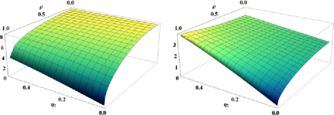
Figure 1: Asymptotic variances of LMM for volatility $\sigma_{1}^{2}$ (left) and co-volatility $\sigma_{12}$ (right) plotted against correlation $\rho$ and noise level $\eta_{2}$ (constant in time).

Figure 1 illustrates the asymptotic variance in the case of volatilities $\sigma^{2}_{1}=\sigma^{2}_{2}=1$ and co-volatility $\sigma_{12}=\rho$ (constant in time) and the first noise level given by $\eta_{1}=1$. The left plot shows the asymptotic variance of the estimator of $\sigma_{1}^{2}$ as a function of $\rho$ and $\eta_{2}$. It is shown that using observations from the other (correlated) process induces clear efficiency gains rising in $\rho$. If the noise level $\eta_{2}$ for the second process is small, the asymptotic variance can even approach zero. The plot on the right shows the same dependence for estimating the co-volatility $\sigma_{12}$. For comparable size of $\eta_{2}$ and $\eta_{1}$ the asymptotic variance increases in $\rho$, which is explained by the fact that also the value to be estimated increases. For small values of $\eta_{2}$, however, the efficiency gain by exploiting the correlation prevails.

For larger dimensions $d$, the variance can even be of order $\mathcal{O}(1/\sqrt{d})$: in the concrete case where all volatilities and noise levels equal $1$, the asymptotic variance for estimating $\sigma_{1}^{2}$ can be reduced from $8$ (using only observations from the first component or if $\Sigma$ is diagonal) down to $8/\sqrt{d}$ (in case of perfect correlation).

All the preceding examples can be worked out for different noise levels $\eta_{p}$. For a fixed entry $(p,q)$, generally all noise levels enter and can be only de-coupled in case of a diagonal covariation matrix $\Sigma=\operatorname{diag}(\sigma_{p}^{2})_{1\leq p\leq d}$. Then the covariance simplifies to

$$p\neq q\dvtx\qquad 2\int_{0}^{1}\bigl{(}\eta_{p}\sigma_{p}\sigma_{q}^{2}+\eta_{q}\sigma_{q}\sigma_{p}^{2}\bigr{)}(t)\,dt;\qquad p=q\dvtx\qquad 8\int_{0}^{1}\bigl{(}\eta_{p}\sigma_{p}^{3}\bigr{)}(t)\,dt.$$

Finally, we can also investigate the estimation of the entire quadratic covariation matrix $\int_{0}^{1}\Sigma(t)\,dt$ under homogeneous noise level and measure its loss by the squared ($d\times d$)-Hilbert–Schmidt norm. Summing up the variances for each entry, we obtain the asymptotic risk

$$\frac{4\eta}{\sqrt{n}}\int_{0}^{1}\bigl{(}\operatorname{trace}\bigl{(}\Sigma^{1/2}\bigr{)}\operatorname{trace}(\Sigma)+\operatorname{trace}\bigl{(}\Sigma^{3/2}\bigr{)}\bigr{)}(t)\,dt.$$

This can be compared with the corresponding Hilbert–Schmidt norm error $\frac{1}{n}(\operatorname{trace}(\Sigma)^{2}+\operatorname{trace}(\Sigma^{2}))$ for the empirical covariance matrix in the i.i.d. Gaussian $\mathbf{N}(0,\Sigma)$-setting.

3 From discrete to continuous-time observations

3.1 Setting

First, let us specify different regularity assumptions. For functions $f\dvtx[0,1]\to\mathbb{R}^{m}$, $m\geq 1$ or also $m=d\times d$ for matrix values, we introduce the $L^{2}$-Sobolev ball of order $\alpha\in(0,1]$ and radius $R>0$ given by

$$H^{\alpha}(R)=\bigl{\{}f\in H^{\alpha}\bigl{(}[0,1],\mathbb{R}^{m}\bigr{)}|\|f\|_{H^{\alpha}}\leq R\bigr{\}}$$

$$\eqntext{\mbox{where }\displaystyle\|f\|_{H^{\alpha}}\mathrel{\mathop{:}}=\max_{1\leq i\leq m}\|f_{i}\|_{H^{\alpha}},}$$ (7)

which for matrices means $\|f\|_{H^{\alpha}}\mathrel{\mathop{:}}=\max_{1\leq i,j\leq d}\|f_{ij}\|_{H^{\alpha}}$. We also consider Hölder spaces $C^{\alpha}([0,1])$ and Besov spaces $B^{\alpha}_{p,q}([0,1])$ of such functions. Canonically, for matrices we use the spectral norm $\|\cdot\|$ and we set $\|f\|_{\infty}\mathrel{\mathop{:}}=\sup_{t\in[0,1]}{\|f(t)\|}$.

In order to pursue asymptotic theory, we impose that the deterministic samplings in each component can be transferred to an equidistant scheme by respective quantile transformations independent of $n_{l},1\leq l\leq d$.

Assumption 3.1 (($\alpha$)).

Suppose that there exist differentiable distribution functions $F_{l}$ with $F_{l}^{\prime}\in C^{\alpha}([0,1])$, $F_{l}(0)=0$, $F_{l}(1)=1$ and $F_{l}^{\prime}>0$ such that the observation times in ($\mathcal{E}_{0}$) are generated by $t_{i}^{(l)}=F_{l}^{-1}(i/n_{l})$, $0\leq i\leq n_{l}$, $1\leq l\leq d$.

We gather all assertions on the instantaneous co-volatility matrix function $\Sigma(t)$, $t\in[0,1]$, which we shall require at some point.

Assumption 3.2.

Let $\Sigma\dvtx[0,1]\to\mathbb{R}^{d\times d}$ be a possibly random function with values in the class of symmetric, positive semi-definite matrices, independent of $X$ and the observational noise, satisfying: [(iii-$\underline{\Sigma}$)]

$\Sigma\in H^{\beta}([0,1])$ for $\beta>0$.

$\Sigma=\Sigma^{B}+\Sigma^{M}$ with $\Sigma^{B}\in B_{1,\infty}^{\alpha}([0,1])$ for $\alpha>0$ and $\Sigma^{M}$ a matrix-valued $L^{2}$-martingale.

$\Sigma(t)\geq\underline{\Sigma}$ for a strictly positive definite matrix $\underline{\Sigma}$ and all $t\in[0,1]$.

We briefly discuss the different function spaces; see, for example, Cohen Cohen , Section 3.2, for a survey. First, any $\alpha$-Hölder-continuous function lies in the $L^{2}$-Sobolev space $H^{\alpha}$ and any $H^{\alpha}$-function lies in the Besov space $B^{\alpha}_{1,\infty}$, where differentiability is measured in an $L^{1}$-sense. The important class of bounded variation functions (e.g., modeling jumps in the volatility) lies in $B^{1}_{1,\infty}$, but only in $H^{\alpha}$ for $\alpha<1/2$. In particular, part (ii-$\alpha$), $\alpha\leq 1$, covers $L^{2}$-semi-martingales by separate bounds on the drift (bounded variation) and martingale part. Beyond classical theory in this area is the fact that also nonsemi-martingales like fractional Brownian motion $B^{H}$ with hurst parameter $H>1/2$ give rise to feasible volatility functions in the results below, using $B^{H}\in C^{H-\varepsilon}\cap B^{H}_{1,\infty}$ for any $\varepsilon>0$ as in Ciesielski et al. Ciesielski .

In the sequel, the potential randomness of $\Sigma$ is often not discussed additionally because by independence we can always work conditionally on $\Sigma$. Finally, let us point out that we could weaken the Hölder-assumptions on $F_{1},\ldots,F_{d}$ toward Sobolev or Besov regularity at the cost of tightening the assumptions on $\Sigma$. For the sake of clarity, this is not pursued here.

Throughout the article, we write $Z_{n}=\mathcal{O}_{P}(\delta_{n})$ and $Z_{n}=\scriptstyle{\mathcal{O}}_{P}(\delta_{n})$ for a sequence of random variables $Z_{n}$ and a sequence $\delta_{n}$, to express that $\delta_{n}^{-1}Z_{n}$ is tight and tends to zero in probability, respectively. Analogously, $\mathcal{O}$ (or equivalently $\lesssim$) and $\scriptstyle{\mathcal{O}}$ refer to deterministic sequences. We write $Z_{n}\asymp Y_{n}$ if $Z_{n}=\mathcal{O}_{P}(Y_{n})$ and $Y_{n}=\mathcal{O}_{P}(Z_{n})$ and the same for deterministic quantities.

3.2 Continuous-time experiment

Definition 3.3.

Let $\mathcal{E}_{0}((n_{l})_{1\leq l\leq d},\beta,R)$ with $n_{l}\in\mathbb{N},\beta\in(0,1],R>0$, be the statistical experiment generated by observations from ($\mathcal{E}_{0}$) with $\Sigma\in H^{\beta}(R)$. Analogously, let $\mathcal{E}_{1}((n_{l})_{1\leq l\leq d},\beta,R)$ be the statistical experiment generated by observing ($\mathcal{E}_{1}$) with the same parameter class.

As we shall establish next, experiments ($\mathcal{E}_{0}$) and ($\mathcal{E}_{1}$) will be asymptotically equivalent as $n_{l}\to\infty,1\leq l\leq d$, at a comparable speed, denoting

$$n_{\mathrm{min}}=\min_{1\leq l\leq d}{n_{l}}\quad\mbox{and}\quad n_{\mathrm{max}}=\max_{1\leq l\leq d}{n_{l}}.$$

Theorem 3.4

Grant Assumption 3.1 with $\alpha=\beta$ on the design. The statistical experiments $\mathcal{E}_{0}((n_{l})_{1\leq l\leq d},\beta,R)$ and $\mathcal{E}_{1}((n_{l})_{1\leq l\leq d},\beta,R)$ are asymptotically equivalent for any $\beta\in(0,1/2]$ and $R>0$, provided $n_{\mathrm{min}}\rightarrow\infty$, $n_{\mathrm{max}}=\scriptstyle{\mathcal{O}}((n_{\mathrm{min}})^{1+\beta})$. More precisely, the Le Cam distance $\Delta$ is of order

$$\Delta\bigl{(}\mathcal{E}_{0}\bigl{(}(n_{l})_{1\leq l\leq d},\beta,R\bigr{)},\mathcal{E}_{1}\bigl{(}(n_{l})_{1\leq l\leq d},\beta,R\bigr{)}\bigr{)}=\mathcal{O}\Biggl{(}R^{2}\Biggl{(}\sum_{l=1}^{d}n_{l}/\eta_{l}^{2}\Biggr{)}n_{\mathrm{min}}^{-1-\beta}\Biggr{)}.$$

By inclusion, the result also applies for $\beta>1/2$ when in the remaining expressions $\beta$ is replaced by $\min(\beta,1/2)$. A standard Sobolev smoothness of $\Sigma$ is $\beta$ almost 1/2 for diffusions with finitely many or absolutely summable jumps. In that case, the asymptotic equivalence result holds if $n_{\mathrm{max}}$ grows more slowly than $n_{\mathrm{min}}^{3/2}$. Theorem 3.4 is proved in the Appendix in a constructive way by warped linear interpolation, which yields a readily implementable procedure; cf. Section 6 below.

4 Localisation and method of moments

4.1 Construction

We partition the interval $[0,1]$ in blocks $[kh,(k+1)h)$ of length $h$. On each block a parametric MLE for a constant model could be sought for. Its numerical determination, however, is difficult and unstable due to the nonconcavity of the ML objective function and its analysis is quite involved. Yet, the likelihood equation leads to spectral statistics whose empirical covariances estimate the quadratic covariation matrix. We therefore prefer a localised method of moments (LMM) for these spectral statistics where for an adaptive version the theoretically optimal weights are determined in a pre-estimation step, in analogy with the classical (multi-step) GMM (generalised method of moments) approach by Hansen Hansen .

As motivated in Section 2, let us consider the local spectral statistics $S_{jk}$ in (4) from the continuous-time experiment ($\mathcal{E}_{1}$). First, we consider a locally constant approximation.

Definition 4.1.

Set $\bar{f}_{h}(t):=h^{-1}\int_{kh}^{(k+1)h}f(s)\,ds$ for $t\in[kh,(k+1)h)$ and a function $f$ on $[0,1]$. Assume $h^{-1}\in\mathbb{N}$ and let $X_{t}^{h}=X_{0}+\int_{0}^{t}\bar{\Sigma}^{{1}/{2}}_{h}(s)\,d{B}_{s}$ with a $d$-dimensional standard Brownian motion ${B}$. Define the process

$$d\tilde{Y}_{t}=X_{t}^{h}\,dt+\operatorname{diag}\Bigl{(}\sqrt{\overline{H}^{2}_{n,l,h}(t)}\Bigr{)}_{1\leq l\leq d}\,d{W}_{t},\qquad t\in[0,1], \mathcal{E}_{2}$$ ()

where ${W}$ is a standard Brownian motion independent of ${B}$ and with noise level (1). The observations from ($\mathcal{E}_{2}$) for $\Sigma\in H^{\beta}(R)$ generate experiment $\mathcal{E}_{2}((n_{l})_{1\leq l\leq d},h,\beta,R)$.

In experiment ($\mathcal{E}_{2}$), we thus observe a process with a co-volatility matrix which is constant on each block $[kh,(k+1)h)$ and corrupted by noise of block-wise constant magnitude. Our approach is founded on the idea that for small block sizes $h$ and sufficient regularity this piecewise constant approximation is close to ($\mathcal{E}_{1}$).

The LMM estimator is built from the data in experiment $\mathcal{E}_{1}$, but designed for the block-wise parametric model ($\mathcal{E}_{2}$). In ($\mathcal{E}_{2}$), the $L^{2}$-orthogonality of $(\varphi_{jk})$ as well as that of $(\Phi_{jk})$ imply (cf. Reiss reiss )

$$S_{jk}\sim\mathbf{N}({0},C_{jk})\qquad\mbox{independent for all }(j,k)$$ (1)

with covariance matrix

$$C_{jk} = \Sigma^{kh}+\pi^{2}j^{2}h^{-2}\operatorname{diag}\bigl{(}H^{kh}_{n,l}\bigr{)}_{l}^{2},\qquad\Sigma^{kh}=\bar{\Sigma}_{h}(kh),$$

$$H^{kh}_{n,l} = \bigl{(}\overline{H}^{2}_{n,l,h}(kh)\bigr{)}^{1/2}.$$

Let us further introduce the Fisher information-type matrices

$$I_{jk}=C_{jk}^{-1}\otimes C_{jk}^{-1},\qquad I_{k}=\sum_{j=1}^{\infty}I_{jk},\qquad j\geq 1,k=0,\ldots,h^{-1}-1.$$

Our local method of moments estimator with oracle weights $\operatorname{LMM}_{\mathrm{or}}^{(n)}$ exploits that on each block a natural second moment estimator of $\Sigma^{kh}$ is given as a convex combination of the bias-corrected empirical covariances:

$$\qquad\operatorname{LMM}_{\mathrm{or}}^{(n)}:=\sum_{k=0}^{h^{-1}-1}h\sum_{j=1}^{\infty}W_{jk}\operatorname{vec}\biggl{(}S_{jk}S_{jk}^{\top}-\frac{\pi^{2}j^{2}}{h^{2}}\operatorname{diag}{\bigl{(}\bigl{(}H_{n,l}^{kh}\bigr{)}^{2}\bigr{)}}_{1\leq l\leq d}\biggr{)}.$$ (3)

The optimal weight matrices $W_{jk}$ in the oracle case are obtained as

$$W_{jk}:=I_{k}^{-1}I_{jk}\in\mathbb{R}^{d^{2}\times d^{2}}.$$ (4)

Note that $C_{jk},I_{jk},I_{k}$ and $W_{jk}$ all depend on $(n_{l})_{1\leq l\leq d}$ and $h$, which is omitted in the notation. Finally, observe that (4.1) and $\sum_{j}W_{jk}=E_{d^{2}}$ imply that $\operatorname{LMM}_{\mathrm{or}}^{(n)}$ is unbiased under model ($\mathcal{E}_{2}$).

4.2 Asymptotic properties of the estimators

We formulate the main result of this section that the oracle estimator (3) and also a fully adaptive version for the quadratic covariation matrix satisfy central limit theorems.

Theorem 4.2

Let Assumptions 3.1($\alpha$), 3.2(ii-$\alpha$) and 3.2(iii-$\underline{\Sigma}$) with $\alpha>1/2$ hold true for observations from model ($\mathcal{E}_{1}$). The oracle estimator (3) yields a consistent estimator for $\operatorname{vec}(\int_{0}^{1}\Sigma(s)\,ds)$ as $n_{\mathrm{min}}\rightarrow\infty$ and $h=h_{0}n_{\mathrm{min}}^{-1/2}$ with $h_{0}\to\infty$. Moreover, if $n_{\mathrm{max}}=\scriptstyle{\mathcal{O}}(n_{\mathrm{min}}^{2\alpha})$ and $h=\scriptstyle{\mathcal{O}}(n_{\mathrm{max}}^{-1/4})$, then a multi-variate central limit theorem holds:

$$\mathbf{I}_{n}^{1/2}\biggl{(}\operatorname{LMM}_{\mathrm{or}}^{(n)}-\operatorname{vec}\biggl{(}\int_{0}^{1}\Sigma(s)\,ds\biggr{)}\biggr{)}\stackrel{{\scriptstyle\mathcal{L}}}{{\longrightarrow}}\mathbf{N}(0,{\mathcal{Z}})\qquad\mbox{in }\mathcal{E}_{1}$$ (5)

with $\mathcal{Z}$ from (6) and $\mathbf{I}_{n}^{-1}=\sum_{k=0}^{h^{-1}-1}h^{2}I_{k}^{-1}$.

While the preceding result is most useful in applications, it is, of course, important to understand the asymptotic covariance structure of the estimator as well; cf. the discussion of efficiency above. Therefore, we consider comparable sample sizes and normalise with $n_{\mathrm{min}}^{1/4}$ in the following result.

Corollary 4.3.

Under the assumptions of Theorem 4.2 suppose$n_{\mathrm{min}}/n_{p}\to\nu_{p}\in(0,1]$ for $p=1,\ldots,d$ and introduce ${\mathcal{H}}(t)=\operatorname{diag}(\eta_{p}\nu_{p}^{1/2}\times F_{p}^{\prime}(t)^{-1/2})_{p}\in\mathbb{R}^{d\times d}$ and $\Sigma_{\mathcal{H}}^{1/2}:={\mathcal{H}}({\mathcal{H}}^{-1}\Sigma{\mathcal{H}}^{-1})^{1/2}{\mathcal{H}}$. Then

$$n_{\mathrm{min}}^{1/4}\biggl{(}\operatorname{LMM}_{\mathrm{or}}^{(n)}-\operatorname{vec}\biggl{(}\int_{0}^{1}\Sigma(s)\,ds\biggr{)}\biggr{)}\stackrel{{\scriptstyle\mathcal{L}}}{{\longrightarrow}}\mathbf{N}\bigl{(}0,\mathbf{I}^{-1}{\mathcal{Z}}\bigr{)}\qquad\mbox{in }\mathcal{E}_{1}$$ (6)

with $\mathbf{I}^{-1}=2\int_{0}^{1}(\Sigma\otimes\Sigma_{\mathcal{H}}^{1/2}+\Sigma_{\mathcal{H}}^{1/2}\otimes\Sigma)(t)\,dt$. In particular, the entries satisfy for $p,q=1,\ldots,d$

$$n_{\mathrm{min}}^{1/4}\biggl{(}\bigl{(}\operatorname{LMM}_{\mathrm{or}}^{(n)}\bigr{)}_{p(d-1)+q}-\int_{0}^{1}\Sigma_{pq}(s)\,ds\biggr{)}$$

$$\qquad\stackrel{{\scriptstyle\mathcal{L}}}{{\longrightarrow}}\mathbf{N}\biggl{(}0,2(1+\delta_{p,q})$$ (7)

$$\hskip 57.0pt{}\times\int_{0}^{1}\bigl{(}\Sigma_{pp}\bigl{(}\Sigma_{\mathcal{H}}^{1/2}\bigr{)}_{qq}+\Sigma_{qq}\bigl{(}\Sigma_{\mathcal{H}}^{1/2}\bigr{)}_{pp}+2\Sigma_{pq}\bigl{(}\Sigma_{\mathcal{H}}^{1/2}\bigr{)}_{pq}\bigr{)}(t)\,dt\biggr{)}.$$

The variance (4.3) will coincide with the lower bound obtained in Section 5 below. The local noise level in ${\mathcal{H}}(t)$ depends on the observational noise level $\eta_{p}$ and the local sample size $\nu_{p}^{-1}F_{p}^{\prime}(t)$, $p=1,\ldots,d$, after normalisation by $n_{\mathrm{min}}$. It is easy to see that in the case $n_{\mathrm{min}}/n_{p}\to 0$ the asymptotic variance vanishes for all entries $(p,q)$, $q=1,\ldots,d$. We infer the structure of the asymptotic covariance matrix using block-wise diagonalisation in Appendix B.

To obtain a feasible estimator, the optimal weight matrices $W_{jk}=W_{j}(\Sigma^{kh})$ and the information-type matrices $I_{jk}=I_{j}(\Sigma^{kh})$ are estimated in a preliminary step from the same data. To reduce variability in the estimate, a coarser grid of $r^{-1}$ equidistant intervals, $r/h\in\mathbb{N}$ is employed for $\hat{W}_{jk}$. As derived in Bibinger and Reiss bibingerreiss for supremum norm loss and extended to $L^{1}$-loss and Besov regularity using the $L^{1}$-modulus of continuity as in the case of wavelet estimators (Corollary 3.3.1 in Cohen Cohen ), a preliminary estimator $\hat{\Sigma}(t)$ of the instantaneous co-volatility matrix $\Sigma(t)$ exists with

$$\|\hat{\Sigma}-\Sigma\|_{L^{1}}=\mathcal{O}_{P}\bigl{(}n_{\mathrm{min}}^{-\alpha/(4\alpha+2)}\bigr{)}$$ (8)

for $\Sigma\in B^{\alpha}_{1,\infty}([0,1])$. For block $k$ with $kh\in[mr,(m+1)r)$, we set

$$\hat{W}_{jk}=W_{j}\bigl{(}\hat{\Sigma}^{mr}\bigr{)},\qquad\hat{I}_{jk}=I_{j}\bigl{(}\hat{\Sigma}^{kh}\bigr{)}\qquad\mbox{with }\hat{\Sigma}^{mr}=\overline{\hat{\Sigma}}_{r}(mr),\hat{\Sigma}^{kh}=\overline{\hat{\Sigma}}_{h}(kh).$$

The LMM estimator with adaptive weights is then given by

$$\qquad\operatorname{LMM}_{\mathrm{ad}}^{(n)}=\sum_{k=0}^{h^{-1}-1}h\sum_{j=1}^{\infty}\hat{W}_{jk}\operatorname{vec}\biggl{(}S_{jk}S_{jk}^{\top}-\frac{\pi^{2}j^{2}}{h^{2}}\operatorname{diag}{\bigl{(}\bigl{(}H_{n,l}^{kh}\bigr{)}^{2}\bigr{)}}_{1\leq l\leq d}\biggr{)}.$$ (9)

We estimate the total covariance matrix via

$$\hat{\mathbf{I}}_{n}^{-1}=\sum_{k=0}^{h^{-1}-1}h^{2}\Biggl{(}\sum_{j=1}^{\infty}\hat{I}_{jk}\Biggr{)}^{-1}.$$ (10)

As $j\to\infty$, the weights $W_{j}(\Sigma)$ and the matrices $I_{j}(\Sigma)$ decay like $j^{-4}$ in norm, compare Lemma C.1 below, such that in practice a finite sum over frequencies $j$ suffices. By a tight bound on the derivatives of $\Sigma\mapsto W_{j}(\Sigma)$, we show in Appendix C.4 the following general result.

Theorem 4.4

Suppose $\Sigma\in B^{\alpha}_{1,\infty}([0,1])$ for $\alpha\in(1/2,1]$ satisfying$\alpha/(2\alpha+1)>\log(n_{\mathrm{max}})/\log(n_{\mathrm{min}})-1.$ Choose $h,r\to 0$ such that $h_{0}=\break hn_{\mathrm{min}}^{1/2}\asymp\log(n_{\mathrm{min}})$ and $n_{\mathrm{min}}^{-\alpha/(2\alpha+1)}\lesssim r\lesssim(n_{\mathrm{min}}/n_{\mathrm{max}})^{1/2}$, $h^{-1},r^{-1},r/h\in\mathbb{N}$. If the pilot estimator $\hat{\Sigma}$ satisfies (8), then under the conditions of Theorem 4.2 the adaptive estimator (9) satisfies

$$\hat{\mathbf{I}}_{n}^{1/2}\biggl{(}\operatorname{LMM}_{\mathrm{ad}}^{(n)}-\operatorname{vec}\biggl{(}\int_{0}^{1}\Sigma(s)\,ds\biggr{)}\biggr{)}\stackrel{{\scriptstyle\mathcal{L}}}{{\longrightarrow}}\mathbf{N}(0,{\mathcal{Z}}),$$ (11)

with $\hat{\mathbf{I}}_{n}$ from (10).

Moreover, Corollary 4.3 applies equally to the adaptive estimator (9).

Since the estimated $\hat{\mathbf{I}}_{n}$ appears in the CLT, we have obtained a feasible limit theorem and (asymptotic) inference statements are immediate.

Some assumptions of Theorem 4.4 are tighter than for the oracle estimator. To some extent this is for the sake of clarity. Here, we have restricted Assumption 3.2(ii-$\alpha$) to the Besov-regular part. A generalisation of the pilot estimator to martingales seems feasible, but is nonstandard and might require additional conditions. We have also proposed a concrete order of $h$ and $r$, less restrictive bounds are used in the proof; see, for example, (27) below.

The lower bound for $\alpha$ in terms of the sample-size ratio $n_{\mathrm{max}}/n_{\mathrm{min}}$ is due to rough norm bounds for (estimated) information-type matrices. For $\alpha=1$ (bounded variation case), the restriction imposes $n_{\mathrm{max}}$ to be slightly smaller than $n_{\mathrm{min}}^{4/3}$. By the Sobolev embedding $B^{1}_{1,\infty}\subseteq H^{\beta}$ for all $\beta<1/2$, the restriction $n_{\mathrm{max}}=\scriptstyle{\mathcal{O}}(n_{\mathrm{min}}^{1+\beta})$ from Theorem 3.4 is clearly also satisfied in this case. It is not clear whether a more elaborate analysis can avoid these restrictions. Still, to the best of our knowledge, a feasible CLT for asymptotically separating sample sizes has not been obtained before.

5 Semi-parametric Cramér–Rao bound

We shall derive an efficiency bound for the following basic case of observation model ($\mathcal{E}_{1}$):

$$dY_{t}=X_{t}\,dt+\frac{1}{\sqrt{n}}\,dW_{t},\qquad X_{t}=\int_{0}^{t}\Sigma(s)^{1/2}\,dB_{s},\qquad t\in[0,1],$$ (12)

where

$$\Sigma(t)=\Sigma_{0}(t)+\varepsilon\mathbb{H}(t),\qquad\Sigma_{0}(t)^{1/2}=O(t)^{\top}\Lambda(t)O(t).$$ (13)

We assume $\Sigma_{0}(t)$ and $\mathbb{H}(t)$ to be known symmetric matrices, $O(t)$ orthogonal matrices, $\Lambda(t)=\operatorname{diag}(\lambda_{1}(t),\ldots,\lambda_{d}(t))$ diagonal and consider $\varepsilon\in[-1,1]$ as unknown parameter. Furthermore, we require Assumption 3.2(iii-$\underline{\Sigma}$) for all $\Sigma$. Finally, we impose throughout this section the regularity assumption that the matrix functions $O(t),\mathbb{H}(t),\Lambda(t)$ are continuously differentiable.

The key idea is to transform the observation of $dY_{t}$ in such a manner that the white noise part remains invariant in law while for the central parameter $\Sigma(t)=\Sigma_{0}(t)$ the process $X$ is transformed to a process with independent coordinates and constant volatility. It turns out that this can only be achieved at the cost of an additional drift in the signal. The construction first rotates the observations via $O(t)$, which diagonalises $\Sigma_{0}(t)$, and then applies a coordinate-wise time-transformation, corrected by a multiplication term to ensure $L^{2}$-isometry such that the white noise remains law-invariant. All proofs are delegated to the supplementary file supplement .

We introduce the coordinate-wise time changes by

$$r_{i}(t)=\frac{\int_{0}^{t}\lambda_{i}(s)\,ds}{\int_{0}^{1}\lambda_{i}(s)\,ds}\quad\mbox{and}\quad(T_{r}g)(t):=\bigl{(}g_{1}\bigl{(}r_{1}(t)\bigr{)},\ldots,g_{d}\bigl{(}r_{d}(t)\bigr{)}\bigr{)}^{\top}$$

for $g=(g_{1},\ldots,g_{d})\dvtx\mathbb{R}\to\mathbb{R}^{d}$. Moreover, we set

$$\bar{\Lambda}:=\int_{0}^{1}\Lambda(s)\,ds,\qquad R^{\prime}(t):=\bar{\Lambda}^{-1}\Lambda(t)=\operatorname{diag}\bigl{(}r_{1}^{\prime}(t),\ldots,r_{d}^{\prime}(t)\bigr{)}.$$

Lemma 5.1.

By transforming $d\bar{Y}=T_{r}^{-1}{\mathcal{M}}_{(R^{\prime})^{-1/2}O}\,dY$, the observation model (12), (13) is equivalent to observing

$$d\bar{Y}(t)=S(t)\,dt+\frac{1}{\sqrt{n}}\,d\bar{W}(t)$$ (14)

with

$$S(t) = T_{r}^{-1}\biggl{(}\bigl{(}R^{\prime}\bigr{)}^{-1}\biggl{(}\int_{0}^{\cdot}\bigl{(}\bigl{(}R^{\prime}\bigr{)}^{-1/2}O\bigr{)}^{\prime}(s)X(s)\,ds$$

$$\hskip 61.0pt{}+\int_{0}^{\cdot}\bigl{(}R^{\prime}(s)\bigr{)}^{-1/2}O(s)\,dX(s)\biggr{)}\biggr{)}(t)$$

for $t\in[0,1]$. At $\varepsilon=0$ the observation $d\bar{Y}(t)$ reduces to

$$\quad\biggl{(}\int_{0}^{t}T_{r}^{-1}\bigl{(}\bigl{(}R^{\prime}\bigr{)}^{-1}\bigl{(}\bigl{(}R^{\prime}\bigr{)}^{-1/2}O\bigr{)}^{\prime}X\bigr{)}(s)\,ds+\bar{\Lambda}\bar{B}(t)\biggr{)}\,dt+\frac{1}{\sqrt{n}}\,d\bar{W}(t).$$ (15)

Here $\bar{W}$ and $\bar{B}$ are Brownian motions obtained from $W$ and $B$, respectively, via rotation and time shift.

If we may forget in (15) the first term, which is a drift term with respect to the martingale part $\bar{\Lambda}\bar{B}(t)$, then the central observation is indeed a constant volatility model in white noise.

Let us introduce the multiplication operator ${\mathcal{M}}_{A}g:=Ag$ and the integration operator $Ig(t)=-\int_{t}^{1}g(s)\,ds$ and its adjoint $I^{\ast}g(t)=-\int_{0}^{t}g(s)\,ds$. The covariance operator $C_{n,\varepsilon}$ on $L^{2}([0,1],\mathbb{R}^{d})$ obtained from observing the differential in (14) is then given by

$$C_{n,\varepsilon}=T_{r}^{\ast}{\mathcal{M}}_{(R^{\prime})^{1/2}O}I^{\ast}{\mathcal{M}}_{\Sigma_{0}+\varepsilon\mathbb{H}}I{\mathcal{M}}_{O^{\top}(R^{\prime})^{1/2}}T_{r}+n^{-1}\mathrm{Id}.$$

The covariance operator $Q_{n,\varepsilon}$ when omitting the drift part is given by

$$Q_{n,\varepsilon}=Q_{n,0}+\varepsilon I^{\ast}T_{r}^{\ast}{\mathcal{M}}_{M}T_{r}I\qquad\mbox{with }M(t):=\bigl{(}\bigl{(}R^{\prime}\bigr{)}^{-1/2}O\mathbb{H}O^{\top}\bigl{(}R^{\prime}\bigr{)}^{-1/2}\bigr{)}(t),$$

where for $\varepsilon=0$ the one-dimensional Brownian motion covariance operator $C_{\mathrm{BM}}=I^{\ast}I$ appears in $Q_{n,0}=\operatorname{diag}(\bar{\lambda}_{ii}C_{\mathrm{BM}}+n^{-1}\mathrm{Id})_{1\leq i\leq d}$.

Standard calculations for the finite-dimensional Gaussian scale model, for example, LehmannCasella , Chapter 6.6, transfer one-to-one to the infinite-dimensional case of observing $\mathbf{N}(0,Q_{n,\varepsilon})$ and yield as Fisher information for the parameter $\varepsilon$ at $\varepsilon=0$ the value $I_{n}^{Q}=\frac{1}{2}\|Q_{n,0}^{-1/2}\dot{Q}_{0}Q_{n,0}^{-1/2}\|_{\mathrm{HS}}^{2}$ because $Q_{n,0}^{-1/2}Q_{n,\varepsilon}Q_{n,0}^{-1/2}$ is differentiable at $\varepsilon=0$ in Hilbert–Schmidt norm. We show by Hilbert–Schmidt calculus, the Feldman–Hajek theorem and the Girsanov theorem that the models with and without drift do not separate:

$$\limsup_{n\to\infty}\bigl{\|}Q_{n,0}^{-1/2}\dot{Q}_{0}Q_{n,0}^{-1/2}-C_{n,0}^{-1/2}\dot{C}_{0}C_{n,0}^{-1/2}\bigr{\|}_{\mathrm{HS}}<\infty.$$ (16)

Consequently, the drift only contributes the negligible order $\mathcal{O}(1)=\scriptstyle{\mathcal{O}}(\sqrt{n})$ to the Fisher information. Analysing $\mathbf{N}(0,Q_{n,\varepsilon})$, we thus establish a semi-parametric Cramér–Rao bound for estimating any linear functional of the co-volatility matrix.

Theorem 5.2

For a continuous matrix-valued function $A\dvtx[0,1]\to\mathbb{R}^{d\times d}$ consider the estimation of

$$\vartheta:=\int_{0}^{1}\bigl{\langle}A(t),\Sigma(t)\bigr{\rangle}_{\mathrm{HS}}\,dt=\int_{0}^{1}\sum_{i,j=1}^{d}A_{ij}(t)\Sigma_{ij}(t)\,dt\in\mathbb{R}.$$ (17)

Then a hardest parametric subproblem in model (12), (13) is obtained for the perturbation of $\Sigma_{0}$ by

$$\mathbb{H}^{\ast}(t)=\bigl{(}\Sigma_{0}\bigl{(}A+A^{\top}\bigr{)}\Sigma_{0}^{1/2}+\Sigma_{0}^{1/2}\bigl{(}A+A^{\top}\bigr{)}\Sigma_{0}\bigr{)}(t).$$

There any estimator $\hat{\vartheta}_{n}$ of $\vartheta$, which is asymptotically unbiased in the sense $\frac{d}{d\vartheta}(\mathbb{E}_{\vartheta}[\hat{\vartheta}_{n}]-\vartheta)\to 0$, satisfies as $n\to\infty$

$$\operatorname{\mathbb{V}ar}_{\varepsilon=0}(\hat{\vartheta}_{n})$$

$$\qquad\geq\frac{(2+\scriptstyle{\mathcal{O}}(1))}{\sqrt{n}}\int_{0}^{1}\bigl{\langle}\bigl{(}\Sigma_{0}\otimes\Sigma_{0}^{1/2}+\Sigma_{0}^{1/2}\otimes\Sigma_{0}\bigr{)}{\mathcal{Z}}\operatorname{vec}(A),{\mathcal{Z}}\operatorname{vec}(A)\bigr{\rangle}(t)\,dt.$$

Further classical efficiency statements like the local asymptotic minimax theorem would require the LAN-property of the parametric subproblem.

6 Implementation and numerical results

6.1 Discrete-time estimator

The construction to transfer discrete-time to continuous-time observations in the proof of Theorem 3.4 paves the way to the discrete approximation of the local spectral statistics (4). Using the interpolated process and integration by parts yields

$$\int\varphi_{jk}(t)\,dY^{(l)}(t)\asymp-\sum_{\nu=1}^{n_{l}}\int_{t_{\nu-1}^{(l)}}^{t_{\nu}^{(l)}}\Phi_{jk}(t)\frac{Y_{\nu}^{(l)}-Y_{\nu-1}^{(l)}}{t_{\nu}^{(l)}-t_{\nu-1}^{(l)}}\,dt.$$

Hence, for discrete-time observations from ($\mathcal{E}_{0}$) we use the local spectral statistics $S_{jk}$ in (2). The noise terms in (4.1) translate from $\mathcal{E}_{1}$ to $\mathcal{E}_{0}$ via substituting $n_{l}^{-1}\int_{kh}^{(k+1)h}(F_{l}^{\prime}(s))^{-1}\,ds$ by $\sum_{\nu:kh\leq t_{\nu}^{(l)}\leq(k+1)h}(t_{\nu}^{(l)}-t_{\nu-1}^{(l)})^{2}$. The discrete sum times $h^{-1}$ can be understood as a block-wise quadratic variation of time in the spirit of Zhang et al. zhangmykland . The bias is discretised analogously. In theory and practice, frequencies $j$ larger than $\log(\eta_{p}^{-1}n^{1/2})$ can be cut off as the size of the weights $W_{j}$ decays rapidly for $j\to\infty$. Different constants in the choice of the block size $h$ do not cause a finite-sample bias, unless the volatility oscillates rapidly over time (in a nonmartingale fashion).

For the adaptive estimator we are in need of local estimates of $n_{l}F_{l}^{\prime}$, $\Sigma$ and estimators for $\eta_{l}^{2},1\leq l\leq d$. It is well known how to estimate noise variances with faster $\sqrt{n_{l}}$-rates; see, for example, Zhang et al. zhangmykland . Local observation densities can be estimated with block-wise quadratic variation of time as above, which then yield estimates $\hat{H}_{n,l}^{kh}$ of $H_{n,l}$ around time $kh$. Uniformly consistent estimators for $\Sigma(t),t\in[0,1]$, are feasible, for example, averaging spectral statistics for $j=1,\ldots,J$ over a set ${\mathcal{K}}_{t}$ of $K$ adjacent blocks containing $t$:

$$\hat{\Sigma}(t)=K^{-1}\sum_{k\in{\mathcal{K}}_{t}}J^{-1}\sum_{j=1}^{J}\bigl{(}S_{jk}S_{jk}^{\top}-\pi^{2}j^{2}h^{-2}\operatorname{diag}\bigl{(}\bigl{(}\hat{H}_{n,l}^{kh}\bigr{)}_{l}^{2}\bigr{)}\bigr{)}.$$ (18)

We refer to Bibinger and Reiss bibingerreiss for details on the nonparametric pilot estimator with $J=1$.

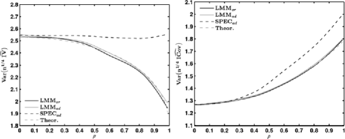
Figure 2: Variances of estimators of $\sigma_{1}^{2}$ (left) and $\sigma_{12}$ (right) in time-constant scenario.

6.2 Simulations

We examine the finite-sample properties of the LMM for the case $d=2$ in two scenarios. First, we compare the finite-sample variance with the asymptotic variances from Sections 3 and 4, for a parametric setup with $\eta_{1}^{2}=\eta_{2}^{2}=0.1$, $\sigma_{1}=\sigma_{2}=1$ and constant correlation $\rho$. We simulate $n_{1}=n_{2}=30\mbox{,}000$ synchronous observations on $[0,1]$. For estimating $\sigma_{1}^{2}$ and $\sigma_{12}=\rho$, Figure 2 displays the rescaled Monte-Carlo variance based on $20\mbox{,}000$ replications of the oracle and adaptive LMM (LMM_or and LMM_ad), as well as the adaptive spectral estimator (SPEC_ad) by Bibinger and Reiss bibingerreiss . The latter relies on the same spectral approach, but uses only scalar weighting instead of the full information matrix approach.

In practice, the pilot estimator from (18) for $J$ not too large performed well. As configuration we use $h^{-1}=10$, $J=30$ and $K=8$, which turned out to be an accurate choice, but the estimators are reasonably robust to alternative input choices. For the LMM of $\sigma_{1}^{2}$, we observe the variance reduction effect associated with a growing signal correlation $\rho$, while the simulation-based variances of both LMM_or and LMM_ad are close to their theoretical asymptotic counterpart (Theor.). The results for $\sigma_{12}$ underline the precision gains compared to SPEC_ad with univariate weights when $\rho$ increases.

Next, we consider a complex and realistic stochastic volatility setting that relies on an extension of the widely-used Heston model as, for example, employed by Aït-Sahalia et al. aitfanxiu2010 , accounting for both leverage effects and an intraday seasonality of volatility. The signal process for $l=1,2$ evolves as

$$dX^{(l)}_{t}=\varphi_{l}(t)\sigma_{l}(t)\,dZ_{t}^{(l)},\qquad d\sigma^{2}_{l}(t)=\alpha_{l}\bigl{(}\mu_{l}-\sigma^{2}_{l}(t)\bigr{)}\,dt+\psi_{l}\sigma_{l}(t)\,dV_{t}^{(l)},$$

where $Z_{t}^{(l)}$ and $V_{t}^{(l)}$ are standard Brownian motions with $dZ_{t}^{(1)}\,dZ_{t}^{(2)}=\rho\,dt$ and $dZ_{t}^{(l)}\,dV_{t}^{(m)}=\delta_{l,m}\gamma_{l}\,dt$. $\varphi_{l}(t)$ is a nonstochastic seasonal factor with $\int_{0}^{1}\varphi_{l}^{2}(t)\,dt=1$. The unit time interval can represent one trading day, for example, 6.5 hours or 23,400 seconds at NYSE.

We initialise the variance process $\sigma^{2}_{l}(t)$ by sampling from its stationary distribution $\Gamma(2\alpha_{l}\mu_{l}/\psi_{l}^{2},\psi_{l}^{2}/(2\alpha_{l}))$ and vary the value of the instantaneous signal correlation $\rho$, while setting $(\mu_{l},\alpha_{l},\psi_{l},\gamma_{l})=(1,6,0.3,-0.3)$, $l=1,2$, which under the stationary distribution, implies $\mathbb{E}[\int_{0}^{1}\varphi_{l}^{2}(t)\sigma^{2}_{l}(t)\,dt]=1$. The seasonal factor $\varphi_{l}(t)$ is specified in terms of intraday volatility functions estimated for S&P 500 equity data by the procedure in Andersen and Bollerslev andbol1997 . $\varphi_{1}(t)$ and $\varphi_{2}(t)$ are based on cross-sectional averages of the 50 most and 50 least liquid stocks, respectively, which yields a pronounced L-shape in both cases (see Figure 3). We add noise processes that are i.i.d. $\mathbf{N}(0,\eta_{l}^{2})$ and mutually independent with $\eta_{l}=0.1(\mathbb{E}[\int_{0}^{1}\varphi_{l}^{4}(t)\sigma^{4}_{l}(t)\,dt])^{1/4}$, computed under the stationary distribution of $\sigma^{2}_{l}(t)$. Finally, asynchronicity effects are introduced by drawing observation times $t_{i}^{(l)}$, $1\leq i\leq n_{l}$, $l=1,2$, from two independent Poisson processes with intensities $\lambda_{1}=1$ and $\lambda_{2}=2/3$ such that, on average, $n_{1}=23\mbox{,}400$ and $n_{2}=15\mbox{,}600$.

Figure 3: Nonstochastic volatility seasonality factors (left) and RMSE for estimators of $\int_{0}^{1}\varphi_{1}^{2}(t)\sigma^{2}_{1}(t)\,dt$ (right) in stochastic volatility scenario.

As a representative example, Figure 3  depicts the root mean-squared errors (RMSEs) based on $40\mbox{,}000$ replications of the following estimators of $\int_{0}^{1}\varphi_{1}^{2}(t)\sigma^{2}_{1}(t)\,dt$: the oracle and adaptive LMM using $h^{-1}=20$, $J=15$ and $K=8$, the quasi-maximum likelihood (QML) estimator by Aït-Sahalia et al. aitfanxiu2010 as well as an oracle version of the widely-used multivariate realised kernel (MRK_or) by Barndorff-Nielsen et al. bn2011 . For the latter, we employ the average univariate mean-squared error optimal bandwidth based on the true value of $\int_{0}^{1}\varphi_{l}^{4}(t)\sigma^{4}_{l}(t)\,dt$, $l=1,2$. Finally, we include the theoretical variance from the asymptotic theory (Theor.), which is computed as the variance (4.3) averaged across all replications.

Three major results emerge. First, the LMM offers considerable precision gains when compared to both benchmarks. Second, a rising instantaneous signal correlation $\rho$ is associated with a declining RMSE of the LMM, which is due to the decreasing variance, and thus confirms the findings from Section 3 in a realistic setting. Finally, the adaptive LMM closely tracks its oracle counterpart.

In summary, the simulation results show that the estimator has promising properties even in settings which are more general than those assumed in ($\mathcal{E}_{1}$), allowing, for instance, for random observation times, stochastic intraday volatility as well as leverage effects. Even if the latter effects are not yet covered by our theory, the proposed estimator seems to be quite robust to deviations from the idealised setting.

Appendix A From discrete to continuous experiments

Proof of Theorem 3.4 To establish Le Cam equivalence, we give a constructive proof to transfer observations in $\mathcal{E}_{0}$ to the continuous-time model $\mathcal{E}_{1}$ and the other way round. We bound the Le Cam distance by estimates for the squared Hellinger distance between Gaussian measures and refer to Section A.1 in reiss for information on Hellinger distances between Gaussian measures and bounds with the Hilbert–Schmidt norm. The crucial difference here is that linear interpolation is carried out for nonsynchronous irregular observation schemes. Consider the linear B-splines or hat functions

$$b_{i,n}(t)=\mathbh{1}_{[{(i-1)}/{n},{(i+1)}/{n}]}(t)\min{\biggl{(}1+n\biggl{(}t-\frac{i}{n}\biggr{)},1-n\biggl{(}t-\frac{i}{n}\biggr{)}\biggr{)}}.$$

Define $b_{i}^{l}(t):=b_{i,n_{l}}(F_{l}(t)),1\leq i\leq n_{l},1\leq l\leq d$, which are warped spline functions satisfying $b_{i_{1}}^{l}(t^{(l)}_{i_{2}})=\delta_{i_{1},i_{2}}$. A centered Gaussian process $\hat{Y}$ is derived from linearly interpolating each component of $Y$:

$$\hat{Y}_{t}^{(l)}=\sum_{i=1}^{n_{l}}{Y}_{i}^{(l)}b_{i}^{l}(t)=\sum_{i=1}^{n_{l}}X_{t_{i}^{(l)}}^{(l)}b_{i}^{l}(t)+\sum_{i=1}^{n_{l}}\mathbf{\varepsilon}^{(l)}_{i}b_{i}^{l}(t).$$ (19)

Setting $A(t)=(a_{lr}(t))_{l,r=1,\ldots,d}=\int_{0}^{t}\Sigma(s)\,ds$, the covariance matrix function $\mathbb{E}[\hat{Y}_{t}{\hat{Y}_{s}}^{\top}]$ of the interpolated process $\hat{Y}$ is determined by

$$\mathbb{E}\bigl{[}\hat{Y}^{(l)}_{t}{\hat{Y}^{(r)}_{s}}\bigr{]}=\sum_{i=1}^{n_{l}}\sum_{\nu=1}^{n_{r}}a_{lr}\bigl{(}t_{i}^{(l)}\wedge t_{\nu}^{(r)}\bigr{)}b_{i}^{l}(t)b_{\nu}^{r}(s)+\delta_{l,r}\eta_{l}^{2}\sum_{i=1}^{n_{l}}b_{i}^{l}(t)b_{i}^{l}(s).$$

For any $g=(g^{(1)},\ldots,g^{(d)})^{\top}\in L^{2}([0,1],\mathbb{R}^{d})$, we have in the $L^{2}$-scalar product

$$\mathbb{E}\bigl{[}\langle{g},\hat{Y}\rangle^{2}\bigr{]}=\sum_{l,r=1}^{d}\sum_{i=1}^{n_{l}}\sum_{\nu=1}^{n_{r}}a_{lr}\bigl{(}t_{i}^{(l)}\wedge t_{\nu}^{(r)}\bigr{)}\bigl{\langle}g^{(l)},b_{i}^{l}\bigr{\rangle}\bigl{\langle}g^{(r)},b_{\nu}^{r}\bigr{\rangle}+\sum_{l=1}^{d}\sum_{i=1}^{n_{l}}\bigl{\langle}g^{(l)},b_{i}^{l}\bigr{\rangle}^{2}\eta_{l}^{2}.$$

The sum of the addends induced by the observation noise in diagonal terms is bounded from above by $\sum_{l=1}^{d}\frac{\eta_{l}^{2}}{n_{l}}\|g^{(l)}/\sqrt{F_{l}^{\prime}}\|_{L^{2}}^{2}=\sum_{l=1}^{d}\|g^{(l)}H_{n,l}\|_{L^{2}}^{2}$ since by virtue of $0\leq\sum_{i}b_{i,n}\leq 1$, $\int b_{i,n}=1/n$ and Jensen’s inequality:

$$\sum_{i=1}^{n_{l}}\bigl{\langle}g^{(l)},b_{i}^{l}\bigr{\rangle}^{2} \leq \frac{1}{n_{l}}\sum_{i=1}^{n_{l}}\int_{0}^{1}\bigl{(}\bigl{(}g^{(l)}\circ F_{l}^{-1}\bigr{)}\cdot\bigl{(}F_{l}^{-1}\bigr{)}^{\prime}\bigr{)}^{2}b_{i,n_{l}}$$

$$\leq \frac{1}{n_{l}}\int_{0}^{1}\bigl{(}\bigl{(}g^{(l)}\circ F_{l}^{-1}\bigr{)}\cdot\bigl{(}F_{l}^{-1}\bigr{)}^{\prime}\bigr{)}^{2}=\frac{1}{n_{l}}\int_{0}^{1}\frac{(g^{(l)})^{2}}{F_{l}^{\prime}}.$$

On the other hand, we have $\mathbb{E}[\langle g,\operatorname{diag}(H_{n,l})_{l}\,dW\rangle]=\sum_{l=1}^{d}\|g^{(l)}H_{n,l}\|_{L^{2}}^{2}$ for a $d$-dimensional standard Brownian motion $W$. Consequently, a process $\bar{Y}$ with continuous-time white noise and the same signal part as $\hat{Y}$ can be obtained by adding uninformative noise. Introduce the process

$$d\bar{Y}=\Biggl{(}\sum_{i=1}^{n_{l}}X_{t_{i}^{(l)}}b_{i}^{l}(t)\Biggr{)}_{1\leq l\leq d}\,dt+\operatorname{diag}\bigl{(}H_{n,l}(t)\bigr{)}_{1\leq l\leq d}\,dW_{t},$$ (20)

and its associated covariance operator $\bar{C}\dvtx L^{2}\rightarrow L^{2}$, given by

$$\bar{C}g(t)=\Biggl{(}\sum_{r=1}^{d}\sum_{i=1}^{n_{l}}\sum_{\nu=1}^{n_{r}}a_{lr}\bigl{(}t_{i}^{(l)}\wedge t_{\nu}^{(r)}\bigr{)}\bigl{\langle}g^{(r)},b_{\nu}^{r}\bigr{\rangle}\Biggr{)}_{1\leq l\leq d}+\bigl{(}H_{n,l}(t)^{2}g^{(l)}(t)\bigr{)}_{1\leq l\leq d}.$$

In fact, it is possible to transfer observations from our original experiment $\mathcal{E}_{0}$ to observations of (20) by adding $\mathbf{N}(0,\bar{C}-\hat{C})$-noise, where $\hat{C}\dvtx L^{2}\rightarrow L^{2}$ is the covariance operator of $\hat{Y}$. Now, consider the covariance operator

$$Cg(t)=\int_{0}^{1}\int_{0}^{t\wedge u}A(s)\,ds\,g(u)\,du+\biggl{(}\frac{\eta_{l}^{2}}{n_{l}F_{l}^{\prime}(t)}g^{(l)}(t)\biggr{)}_{1\leq l\leq d},$$

associated with the continuous-time experiment $\mathcal{E}_{1}$.

We can bound $C^{-1/2}$ on $L^{2}([0,1],\mathbb{R}^{d})$ from below (by partial ordering of operators) by a simple matrix multiplication operator: $C^{-1/2}\leq{\mathcal{M}}_{\operatorname{diag}(H_{n,l}(t))_{l}}$. Denote the Hilbert–Schmidt or Frobenius norm by $\|\cdot\|_{\mathrm{HS}}$. The asymptotic equivalence of observing $\bar{Y}$ and $Y$ in $\mathcal{E}_{1}$ is ensured by the Hellinger distance bound

$$\operatorname{H}^{2}\bigl{(}\mathcal{L}(\bar{Y}),\mathcal{L}(Y)\bigr{)}$$

$$\qquad\leq 2\bigl{\|}C^{-{1}/{2}}(\bar{C}-C)C^{-{1}/{2}}\bigr{\|}^{2}_{\mathrm{HS}}$$

$$\qquad\leq 2\int_{0}^{1}\int_{0}^{1}\Biggl{(}\sum_{l=1}^{d}\sum_{r=1}^{d}H_{n,l}(t)^{-2}H_{n,r}(t)^{-2}$$

$$\quad\qquad\hskip 40.0pt{}\times\Biggl{(}\sum_{i=1}^{n_{l}}\sum_{\nu=1}^{n_{r}}a_{lr}\bigl{(}t_{i}^{(l)}\wedge t_{\nu}^{(r)}\bigr{)}b_{i}^{l}(t)b_{\nu}^{r}(s)-a_{lr}(t\wedge s)\Biggr{)}^{2}\Biggr{)}\,dt\,ds$$

$$\qquad=2\int_{0}^{1}\int_{0}^{1}\Biggl{(}\sum_{l=1}^{d}\sum_{r=1}^{d}\frac{n_{l}n_{r}}{\eta_{l}^{2}\eta_{r}^{2}}$$

$$\hskip 40.0pt\qquad\quad{}\times\Biggl{(}\sum_{i=1}^{n_{l}}\sum_{\nu=1}^{n_{r}}a_{lr}\bigl{(}t_{i}^{(l)}\wedge t_{\nu}^{(r)}\bigr{)}b_{i,n_{l}}(u)b_{\nu,n_{r}}(z)$$

$$\hskip 140.0pt{}-a_{lr}\bigl{(}F_{l}^{-1}(u)\wedge F_{r}^{-1}(z)\bigr{)}\Biggr{)}^{2}\Biggr{)}\,du\,dz$$

$$\qquad={\mathcal{O}}\Biggl{(}R^{4}\sum_{l=1}^{d}\sum_{r=1}^{d}\eta_{l}^{-2}\eta_{r}^{-2}n_{l}n_{r}n_{\mathrm{min}}^{-2-2\beta}\Biggr{)}.$$

The estimate for the $L^{2}$-distance between the function $(t,s)\mapsto A(F_{l}^{-1}(t)\wedge F_{r}^{-1}(s)),(l,r)\in\{1,\ldots,d\}^{2}$, and its coordinate-wise linear interpolation by $\mathcal{O}(n_{\mathrm{min}}^{-1-\beta}\vee n_{\mathrm{min}}^{-3/2})$ relies on a standard approximation result on a rectangular grid of maximal width $(n_{\mathrm{min}})^{-1}$ based on the fact that this function lies in the Sobolev class $H^{1+\beta}([0,1]^{2})$ with corresponding norm bounded by $2R^{4}$. This follows immediately by the product rule from $A^{\prime}=\Sigma\in H^{\beta}$ and $(F_{l}^{-1})^{\prime}\in C^{\beta}$, together with an $L^{2}$-error bound at the skewed diagonal $\{(t,s)\dvtx F_{l}(t)=F_{r}(s)\}$.

Next, we explicitly show that $\mathcal{E}_{1}$ is at least as informative as $\mathcal{E}_{0}$. To this end, we discretise in each component on the intervals $I_{i,l}=[\frac{i}{n_{l}}-\frac{1}{2n_{l}},\frac{i}{n_{l}}+\frac{1}{2n_{l}}]\cap[0,1]$ for $i=0,\ldots,n_{l}$. Define

$$\qquad\bigl{(}Y_{i}^{\prime}\bigr{)}^{(l)} = \frac{1}{|I_{i,l}|}\int_{F_{l}^{-1}(I_{i,l})}F_{l}^{\prime}(t)\,dY^{(l)}_{t}=\frac{1}{|I_{i,l}|}\int_{F_{l}^{-1}(I_{i,l})}X_{t}^{(l)}F_{l}^{\prime}(t)\,dt+\varepsilon_{i}^{(l)}$$

$$= \frac{1}{|I_{i,l}|}\int_{I_{i,l}}X_{F^{-1}(u)}^{(l)}\,du+\varepsilon_{i}^{(l)},$$

with i.i.d. $\mathbf{N}(0,\eta_{l}^{2})$-random variables $\varepsilon_{i}^{(l)}=\frac{1}{|I_{i,l}|}\int_{F_{l}^{-1}(I_{i,l})}\eta_{l}(F_{l}^{\prime}/n_{l})^{1/2}\,dW_{t}^{(l)}$. The covariances are calculated as

$$\mathbb{E}\bigl{[}\bigl{(}Y_{i}^{\prime}\bigr{)}^{(l)}\bigl{(}Y_{\nu}^{\prime}\bigr{)}^{(r)}\bigr{]}=\frac{1}{|I_{i,l}||I_{\nu,r}|}\int_{I_{i,l}}\int_{I_{\nu,r}}a_{lr}\bigl{(}F_{l}^{-1}(u)\wedge F_{r}^{-1}\bigl{(}u^{\prime}\bigr{)}\bigr{)}\,du\,du^{\prime}+\delta_{l,r}\delta_{i,\nu}\eta_{l}^{2}.$$

We obtain for the squared Hellinger distance between the laws of observation

$$\operatorname{H}^{2}\bigl{(}\mathcal{L}\bigl{(}\bigl{(}Y_{i}^{(l)}\bigr{)}_{l=1,\ldots,d;i=0,\ldots,n_{l}}\bigr{)},\mathcal{L}\bigl{(}\bigl{(}\bigl{(}Y_{i}^{\prime}\bigr{)}^{(l)}\bigr{)}_{l=1,\ldots,d;i=0,\ldots,n_{l}}\bigr{)}\bigr{)}$$

$$\qquad\leq\sum_{l,r=1}^{d}\eta_{l}^{-2}\eta_{r}^{-2}\sum_{i=0}^{n_{l}}\sum_{\nu=0}^{n_{r}}\biggl{(}\frac{1}{|I_{i,l}||I_{\nu,r}|}\int_{I_{i,l}}\int_{I_{\nu,r}}a_{lr}\bigl{(}F_{l}^{-1}(u)\wedge F_{r}^{-1}\bigl{(}u^{\prime}\bigr{)}\bigr{)}$$

$$\hskip 170.0pt{}-a_{lr}\bigl{(}F_{l}^{-1}(i/n_{l}\wedge\nu/n_{r})\bigr{)}\,du\,du^{\prime}\biggr{)}^{2}.$$

Write $A^{F}_{lr}(u,u^{\prime})=a_{lr}(F_{l}^{-1}(u)\wedge F_{r}^{-1}(u^{\prime}))$ and note $A^{F}_{lr}\in H^{1+\beta}([0,1]^{2})$ due to $A^{\prime}=\Sigma\in H^{\beta}$ and $F_{l}^{-1},F_{r}^{-1}\in C^{\beta}$. For $(i,\nu)\notin{\mathcal{C}}:=\{(0,0),(0,n_{r}),(n_{l},0),$ $(n_{l},n_{r})\}$ the rectangle $I_{i,l}\times I_{\nu,r}$ is symmetric around $(i/n_{l},\nu/n_{r})$ such that the integral in the preceding display equals ($\nabla$ denotes the gradient)

$$\int_{I_{i,l}\times I_{\nu,r}}\int_{0}^{1}\biggl{(}\biggl{\langle}\nabla A^{F}_{lr}\biggl{(}\frac{i}{n_{l}}+\vartheta\biggl{(}u-\frac{i}{n_{l}}\biggr{)},\frac{\nu}{n_{r}}+\vartheta\biggl{(}u^{\prime}-\frac{\nu}{n_{r}}\biggr{)}\biggr{)},$$

$$\hskip 160.0pt\qquad{}\biggl{(}u-\frac{i}{n_{l}},u^{\prime}-\frac{\nu}{n_{r}}\biggr{)}\biggr{\rangle}$$

$$\hskip 72.0pt\qquad{}-\biggl{\langle}\nabla A^{F}_{lr}\biggl{(}\frac{i}{n_{l}},\frac{\nu}{n_{r}}\biggr{)},\biggl{(}u-\frac{i}{n_{l}},u^{\prime}-\frac{\nu}{n_{r}}\biggr{)}\biggr{\rangle}\biggr{)}\,d\vartheta\,du\,du^{\prime}.$$

Using Jensen’s inequality, we thus obtain further the bound for the squared Hellinger distance:

$$\sum_{l,r=1}^{d}\eta_{l}^{-2}\eta_{r}^{-2}\sum_{i=0}^{n_{l}}\sum_{\nu=0}^{n_{r}}\frac{(n_{l}\vee n_{r})^{-2}}{|I_{i,l}||I_{\nu,r}|}$$

$$\qquad{}\times\int_{I_{i,l}\times I_{\nu,r}}\int_{0}^{1}\bigl{\|}\nabla A^{F}_{lr}\bigl{(}i/n_{l}+\vartheta(u-i/n_{l}),\nu/n_{r}+\vartheta\bigl{(}u^{\prime}-\nu/n_{r}\bigr{)}\bigr{)}$$

$$\hskip 153.0pt{}-\nabla A^{F}_{lr}(i/n_{l},\nu/n_{r})\mathbh{1}\bigl{(}(i,\nu)\notin{\mathcal{C}}\bigr{)}\bigr{\|}^{2}\,d\vartheta\,du\,du^{\prime}$$

$$\qquad=\sum_{l,r=1}^{d}\eta_{l}^{-2}\eta_{r}^{-2}\frac{n_{l}n_{r}}{(n_{l}\vee n_{r})^{2}}\mathcal{O}\bigl{(}R^{4}(n_{l}\wedge n_{r})^{-2\beta}\bigr{)}$$

$$\qquad=\mathcal{O}\Biggl{(}R^{4}\Biggl{(}\sum_{l=1}^{d}n_{l}/\eta_{l}^{2}\Biggr{)}^{2}n_{\mathrm{min}}^{-2-2\beta}\Biggr{)},$$

where the order estimate is due to $\|\nabla A^{F}_{lr}\|_{H^{\beta}}\leq R^{2}$ and a standard $L^{2}$-approximation result for Sobolev spaces, observing that for the four corner rectangles in $\mathcal{C}$ the boundedness of the respective integrals only adds the total order $4n_{\mathrm{min}}^{-2}<n_{l}n_{r}n_{\mathrm{min}}^{-2-2\beta}$.

Appendix B Asymptotics in the block-wise constant experiment

Proof of Theorem 4.2 As we have seen, the estimator is unbiased in $\mathcal{E}_{2}$. For the covariance structure we use the independence between blocks and frequencies and the commutativity with $\mathcal{Z}$ to infer

$$\operatorname{\mathbb{C}OV}_{\mathcal{E}_{2}}\bigl{(}{\mathbf{I}}_{n}^{1/2}\operatorname{LMM}_{\mathrm{or}}^{(n)}\bigr{)}$$

$$\qquad={\mathbf{I}}_{n}^{1/2}\sum_{k=0}^{h^{-1}-1}h^{2}\sum_{j=1}^{\infty}W_{jk}\operatorname{\mathbb{C}OV}_{\mathcal{E}_{2}}\bigl{(}\operatorname{vec}\bigl{(}S_{jk}S_{jk}^{\top}\bigr{)}\bigr{)}W_{jk}^{\top}{\mathbf{I}}_{n}^{1/2}$$ (22)

$$\qquad={\mathbf{I}}_{n}^{1/2}\sum_{k=0}^{h^{-1}-1}h^{2}I_{k}^{-1}{\mathbf{I}}_{n}^{1/2}{\mathcal{Z}}={\mathcal{Z}}.$$

Since the local Fisher-type information matrices are strictly positive definite, and thus invertible by Assumption 3.2(iii), the multivariate CLT (5) for the oracle estimator follows by applying a standard CLT for triangular schemes as Theorem 4.12 from kallenberg . The Lindeberg condition is implied by the stronger Lyapunov condition which is easily verified here by bounding moments of order $4$.

In Appendix C below, we prove that in experiment ${\mathcal{E}}_{1}$ the estimator $\operatorname{LMM}_{\mathrm{or}}^{(n)}$ has an additional bias of order $\mathcal{O}(n_{\mathrm{min}}^{-\alpha/2})+\mathcal{O}_{P}(h)$ and a difference in the covariance of order $\mathcal{O}(hn_{\mathrm{min}}^{-\alpha/2})+\mathcal{O}_{P}(h^{2})$ under our Assumption 3.2(ii-$\alpha$), (iii-$\underline{\Sigma}$), which by Slutsky’s lemma yields an asymptotically negligible term compared to the best attainable rate (in any entry) $n_{\mathrm{max}}^{-1/4}$; cf. Theorem 5.2.

Proof of Corollary 4.3 An important property of our oracle estimator is its equi-variance with respect to invertible linear transformations $A_{k}$ on each block $k$ in the sense that for observed statistics $\tilde{S}_{jk}:=A_{k}S_{jk}\sim\mathbf{N}(0,\tilde{C}_{jk})$ under $\mathcal{E}_{2}$ we obtain [$A^{-\top}:=(A^{\top})^{-1}$ for short]

$$C_{jk} = A_{k}^{-1}\tilde{C}_{jk}A_{k}^{-\top},\qquad I_{jk}=(A_{k}\otimes A_{k})^{\top}\tilde{I}_{jk}(A_{k}\otimes A_{k}),$$

$$I_{k} = (A_{k}\otimes A_{k})^{\top}\tilde{I}_{k}(A_{k}\otimes A_{k})$$

and hence with some (deterministic) bias correction terms $B_{jk},\tilde{B}_{jk}$

$$\operatorname{LMM}_{\mathrm{or}}^{(n)} = \sum_{k=0}^{h^{-1}-1}h(A_{k}\otimes A_{k})^{-1}\tilde{I}_{k}^{-1}\sum_{j\geq 0}\tilde{I}_{jk}(A_{k}\otimes A_{k})\operatorname{vec}\bigl{(}S_{jk}S_{jk}^{\top}-B_{jk}\bigr{)}$$

$$= \sum_{k=0}^{h^{-1}-1}(A_{k}\otimes A_{k})^{-1}\biggl{(}h\tilde{I}_{k}^{-1}\sum_{j\geq 0}\tilde{I}_{jk}\operatorname{vec}\bigl{(}\tilde{S}_{jk}\tilde{S}_{jk}^{\top}-\tilde{B}_{jk}\bigr{)}\biggr{)}.$$

For the covariance, we use commutativity with $\mathcal{Z}$ and obtain likewise

$$\operatorname{\mathbb{C}OV}_{\mathcal{E}_{2}}\bigl{(}\operatorname{LMM}_{\mathrm{or}}^{(n)}\bigr{)}=\sum_{k=0}^{h^{-1}-1}h^{2}(A_{k}\otimes A_{k})^{-1}\tilde{I}_{k}^{-1}(A_{k}\otimes A_{k})^{-\top}{\mathcal{Z}}.$$ (23)

We use this property to diagonalise the problem on each block. In terms of the noise level matrix ${\mathcal{H}}_{k}:=\operatorname{diag}(H_{l,n}^{k})_{l=1,\ldots,d}$, let $O_{k}$ be an orthogonal matrix such that

$$\Lambda^{kh}=O_{k}\mathcal{H}_{k}^{-1}\Sigma^{kh}\mathcal{H}_{k}^{-1}O_{k}^{\top}$$ (24)

is diagonal. Note that $\Lambda^{kh}$ grows with $n$, but we drop the dependence on $n$ in the notation for all matrices $\Lambda^{kh}$, $O_{k}$ and ${\mathcal{H}}_{k}$. Use $A_{k}=O_{k}\mathcal{H}_{k}^{-1}$ to obtain the spectral statistics (4) transformed:

$$\tilde{S}_{jk}=O_{k}\mathcal{H}_{k}^{-1}S_{jk}\sim\mathbf{N}(\mathbf{0},\tilde{C}_{jk})\qquad\mbox{independent for all }(j,k),$$

which yields a simple-structured diagonal covariance matrix:

$$\tilde{C}_{jk}=O_{k}\mathcal{H}_{k}^{-1}C_{jk}\mathcal{H}_{k}^{-1}O_{k}^{\top}=\Lambda^{kh}+\frac{\pi^{2}j^{2}}{h^{2}}E_{d}.$$

A key point is that the covariance structure (23) in $\mathbb{R}^{d^{2}\times d^{2}}$ is for independent components $\tilde{S}_{jk}$ also diagonal, up to symmetry in the co-volatilitymatrix entries. Summing $\tilde{I}_{jk}$ over $j$ is explicitly solvable and givesfor $p,q=1,\ldots,d$

$$\bigl{(}h\tilde{I}_{k}^{-1}\bigr{)}_{p,q} = \Biggl{(}h^{-1}\sum_{j=1}^{\infty}\bigl{(}\tilde{C}_{jk}^{-1}\otimes\tilde{C}_{jk}^{-1}\bigr{)}_{p,q}\Biggr{)}^{-1}$$

$$= \Biggl{(}h^{-1}\sum_{j=1}^{\infty}\bigl{(}\Lambda_{pp}^{kh}+\pi^{2}j^{2}h^{-2}\bigr{)}^{-1}\bigl{(}\Lambda_{qq}^{kh}+\pi^{2}j^{2}h^{-2}\bigr{)}^{-1}\Biggr{)}^{-1}$$

$$= \biggl{(}\frac{\sqrt{\Lambda_{qq}^{kh}}\coth(h\sqrt{\Lambda_{pp}^{kh}})-\sqrt{\Lambda_{pp}^{kh}}\coth(h\sqrt{\Lambda_{qq}^{kh}})}{2\sqrt{\Lambda_{pp}^{kh}\Lambda_{qq}^{kh}}(\Lambda_{qq}^{kh}-\Lambda_{pp}^{kh})}-\frac{1}{2h\Lambda_{pp}^{kh}\Lambda_{qq}^{kh}}\biggr{)}^{-1}$$

$$= 2\Bigl{(}\Lambda_{pp}^{kh}\sqrt{\Lambda_{qq}^{kh}}+\Lambda_{qq}^{kh}\sqrt{\Lambda_{pp}^{kh}}\Bigr{)}$$

$${}\times\bigl{(}1+\mathcal{O}\bigl{(}e^{-2h\sqrt{\Lambda_{pp}^{kh}\wedge\Lambda_{qq}^{kh}}}+h^{-1}\bigl{(}\Lambda_{pp}^{kh}\wedge\Lambda_{qq}^{kh}\bigr{)}^{-1/2}\bigr{)}\bigr{)},$$

using $\Lambda^{kh}\geq(\min_{l,t}n_{l}F_{l}^{\prime}(t)\eta_{l}^{-2})\underline{\Sigma}\gtrsim n_{\mathrm{min}}E_{d}$, $h^{2}n_{\mathrm{min}}\to\infty$ and $\coth(x)=1+\mathcal{O}(e^{-2x})$ for $x\to\infty$. We thus obtain uniformly over $k$

$$h\tilde{I}_{k}^{-1}=\bigl{(}2+\scriptstyle{\mathcal{O}}(1)\bigr{)}\bigl{(}\Lambda^{kh}\otimes\sqrt{\Lambda^{kh}}+\sqrt{\Lambda^{kh}}\otimes\Lambda^{kh}\bigr{)}.$$

By formula (23), we infer in terms of $(\Sigma_{\mathcal{H}}^{kh})^{1/2}:={\mathcal{H}}_{k}({\mathcal{H}}_{k}^{-1}\Sigma^{kh}{\mathcal{H}}_{k}^{-1})^{1/2}{\mathcal{H}}_{k}$

$$\operatorname{\mathbb{C}OV}_{\mathcal{E}_{2}}\bigl{(}\operatorname{LMM}_{\mathrm{or}}^{(n)}\bigr{)}=\bigl{(}2+\scriptstyle{\mathcal{O}}(1)\bigr{)}\sum_{k=0}^{h^{-1}-1}h\bigl{(}\Sigma^{kh}\otimes\bigl{(}\Sigma_{\mathcal{H}}^{kh}\bigr{)}^{1/2}+\bigl{(}\Sigma_{\mathcal{H}}^{kh}\bigr{)}^{1/2}\otimes\Sigma^{kh}\bigr{)}{\mathcal{Z}}.$$

The final step consists in combining $n_{\mathrm{min}}^{1/2}H_{n,l}(t)\to H_{l}(t)$ uniformly in $t$ together with a Riemann sum approximation to conclude

$$\lim_{n_{\mathrm{min}}\to\infty}n_{\mathrm{min}}^{1/2}\operatorname{\mathbb{C}OV}_{\mathcal{E}_{2}}\bigl{(}\operatorname{LMM}_{\mathrm{or}}^{(n)}\bigr{)}$$

$$\qquad=2\biggl{(}\int_{0}^{1}\bigl{(}\Sigma\otimes\bigl{(}{\mathcal{H}}\bigl{(}{\mathcal{H}}^{-1}\Sigma{\mathcal{H}}^{-1}\bigr{)}^{1/2}{\mathcal{H}}\bigr{)}$$

$$\hskip 59.0pt{}+\bigl{(}{\mathcal{H}}\bigl{(}{\mathcal{H}}^{-1}\Sigma{\mathcal{H}}^{-1}\bigr{)}^{1/2}{\mathcal{H}}\bigr{)}\otimes\Sigma\bigr{)}(t)\,dt\biggr{)}{\mathcal{Z}}.$$

Appendix C Proofs for continuous models

C.1 Weight matrix estimates

We shall often need general norm bounds on the weight matrices $W_{jk}$.

Lemma C.1.

The oracle weight matrices satisfy $\|W_{jk}\|\lesssim h_{0}^{-1}(1+j^{4}/h_{0}^{4})^{-1}$ uniformly over $(j,k)$ and matrices $\Sigma^{kh}$ with $\|\Sigma^{kh}\|_{\infty}+\|(\Sigma^{kh})^{-1}\|_{\infty}\lesssim 1$.

From the proof of Corollary 4.3, we infer

$$W_{jk}=\bigl{(}H_{k}O_{k}^{\top}\otimes H_{k}O_{k}^{\top}\bigr{)}\tilde{W}_{jk}\bigl{(}O_{k}H_{k}^{-1}\otimes O_{k}H_{k}^{-1}\bigr{)}$$

with

$$\tilde{W}_{jk}=\bigl{(}2+\scriptstyle{\mathcal{O}}(1)\bigr{)}h^{-1}\bigl{(}\bigl{(}\Lambda^{kh}\tilde{C}_{jk}^{-1}\bigr{)}\otimes\bigl{(}\sqrt{\Lambda^{kh}}\tilde{C}_{jk}^{-1}\bigr{)}+\bigl{(}\sqrt{\Lambda^{kh}}\tilde{C}_{jk}^{-1}\bigr{)}\otimes\bigl{(}\Lambda^{kh}\tilde{C}_{jk}^{-1}\bigr{)}\bigr{)}.$$

We evaluate one factor in $W_{jk}$ using

$$\bigl{\|}H_{k}O_{k}^{\top}\Lambda^{kh}\tilde{C}_{jk}^{-1}O_{k}H_{k}^{-1}\bigr{\|}=\bigl{\|}\Sigma^{kh}\bigl{(}\Sigma^{kh}+\pi^{2}j^{2}h^{-2}H_{k}^{2}\bigr{)}^{-1}\bigr{\|}\lesssim\bigl{(}1+j^{2}h^{-2}n_{\mathrm{min}}^{-2}\bigr{)}^{-1}.$$

By $\|A\otimes B\|\leq\|A\|\|B\|$ and $\sqrt{\Lambda^{kh}}\tilde{C}_{jk}^{-1}=(\Lambda^{kh}\tilde{C}_{jk}^{-1})(\Lambda^{kh})^{-1/2}$ (the matrices are diagonal), we infer $\|W_{jk}\|\lesssim h^{-1}(1+j^{2}h_{0}^{-2})^{-2}\|H_{k}O_{k}^{\top}(\Lambda^{kh})^{-1/2}O_{k}H_{k}^{-1}\|$. To evaluate the last norm, despite matrix multiplication is noncommutative, we note

$$\bigl{(}O_{k}^{\top}\bigl{(}\Lambda^{kh}\bigr{)}^{-1/2}O_{k}H_{k}^{-1}\bigr{)}^{\top}O_{k}^{\top}\bigl{(}\Lambda^{kh}\bigr{)}^{-1/2}O_{k}H_{k}^{-1} = H_{k}^{-1}O_{k}^{\top}\bigl{(}\Lambda^{kh}\bigr{)}^{-1}O_{k}H_{k}^{-1}$$

$$= \bigl{(}\Sigma^{kh}\bigr{)}^{-1},$$

whence by polar decomposition $|O_{k}^{\top}(\Lambda^{kh})^{-1/2}O_{k}H_{k}^{-1}|=(\Sigma^{kh})^{-1/2}$ implies

$$\bigl{\|}O_{k}^{\top}\bigl{(}\Lambda^{kh}\bigr{)}^{-1/2}O_{k}H_{k}^{-1}\bigr{\|}=\bigl{\|}\bigl{(}\Sigma^{kh}\bigr{)}^{-1/2}\bigr{\|}\lesssim 1.$$

Together with $\|H_{k}\|\lesssim n_{\mathrm{min}}^{-1/2}$ this yields $\|W_{jk}\|\lesssim h^{-1}(1+j^{2}h_{0}^{-2})^{-2}n_{\mathrm{min}}^{-1/2}$, which gives the result.

Moreover, for the adaptive estimator we have to control the dependence of the weight matrices $W_{jk}=W_{j}(\Sigma^{kh})$ on $\Sigma^{kh}$. We use the notion of matrix differentiation as introduced in fackler : define the derivative $dA/dB$ of a matrix-valued function $A(B)\in\mathbb{R}^{o\times p}$ with respect to $B\in\mathbb{R}^{q\times r}$ as the $\mathbb{R}^{op\times qr}$ matrix with row vectors $(d/dB_{ab})\operatorname{vec}(A),1\leq a\leq q,1\leq b\leq r$.

Lemma C.2.

For the derivatives of the oracle weight matrices $W_{j}(\Sigma^{kh})$, assuming $\|\Sigma^{kh}\|_{\infty}+\|(\Sigma^{kh})^{-1}\|_{\infty}\lesssim 1$, we have uniformly over $(j,k)$:

$$\biggl{\|}\frac{d}{d\Sigma^{kh}}W_{j}\bigl{(}\Sigma^{kh}\bigr{)}\biggr{\|}\lesssim h_{0}^{-1}\bigl{(}1+j^{4}h_{0}^{-4}\bigr{)}^{-1}.$$ (25)

Since the notion of matrix derivatives relies on vectorisation, the identities $\operatorname{vec}(I_{k}^{-1}I_{jk})=(E_{d^{2}}\otimes I_{k}^{-1})\operatorname{vec}(I_{jk})=(I_{jk}^{\top}\otimes E_{d^{2}})\operatorname{vec}(I_{k}^{-1})$ give rise to the matrix differentiation product rule

$$\frac{d}{d\Sigma^{kh}}W_{jk}=(I_{jk}\otimes E_{d^{2}})\frac{dI_{k}^{-1}}{d\Sigma^{kh}}+\bigl{(}E_{d^{2}}\otimes I_{k}^{-1}\bigr{)}\frac{dI_{jk}}{d\Sigma^{kh}}.$$ (26)

Applying the mixed product rule $(A\otimes B)(C\otimes D)=(AC\otimes BD)$ repeatedly, and the differentiation product rule and chain rule to $I_{jk}=C_{jk}^{-1}\otimes C_{jk}^{-1}$, we obtain

$$\frac{d}{dC_{jk}}\bigl{(}C_{jk}^{-1}\otimes C_{jk}^{-1}\bigr{)}$$

$$\qquad=-\bigl{(}\bigl{(}C_{jk}^{-1}\otimes C_{jk}^{-1}\bigr{)}\otimes\bigl{(}C_{jk}^{-1}\otimes C_{jk}^{-1}\bigr{)}\bigr{)}$$

$$\qquad\quad{}\times\bigl{(}\bigl{(}(C_{jk}\otimes E_{d}\otimes E_{d^{2}})+(E_{d^{2}}\otimes E_{d}\otimes C_{jk})\bigr{)}(E_{d}\otimes C_{d,d}\otimes E_{d})$$

$$\hskip 100.0pt\qquad\quad{}\times\bigl{(}\bigl{(}\operatorname{vec}(E_{d})\otimes E_{d^{2}}\bigr{)}+\bigl{(}E_{d^{2}}\otimes\operatorname{vec}(E_{d})\bigr{)}\bigr{)}\bigr{)},$$

with the so-called commutation matrix $C_{d,d}=\mathcal{Z}-E_{d^{2}}$. By orthogonality of the last factors in both addends, $\|A\otimes B\|=\|A\|\|B\|$, and the mixed product rule, we infer for the norm of the second addend in (26)

$$\biggl{\|}\bigl{(}E_{d^{2}}\otimes I_{k}^{-1}\bigr{)}\frac{dI_{jk}}{d\Sigma^{kh}}\biggr{\|} \leq 2\bigl{\|}\bigl{(}E_{d}\otimes C_{jk}^{-1}\bigr{)}\otimes\bigl{(}I_{k}^{-1}\bigl{(}C_{jk}^{-1}\otimes C_{jk}^{-1}\bigr{)}\bigr{)}\bigr{\|}$$

$$= 2\|W_{jk}\|\bigl{\|}C_{jk}^{-1}\bigr{\|}\lesssim\|W_{jk}\|.$$

By virtue of $(I_{k}^{-1}\otimes E_{d^{2}})\frac{dI_{k}}{d\Sigma^{kh}}=-(E_{d^{2}}\otimes I_{k})\frac{dI_{k}^{-1}}{d\Sigma^{kh}}$ it follows with the mixed product rule that $dI_{k}^{-1}/d\Sigma^{kh}=-(I_{k}^{-1}\otimes I_{k}^{-1})(dI_{k}/d\Sigma^{kh})$. This yields for the norm of the first addend in (26)

$$\biggl{\|}(I_{jk}\otimes E_{d^{2}})\frac{dI_{k}^{-1}}{d\Sigma^{kh}}\biggr{\|} = \biggl{\|}\bigl{(}W_{jk}^{\top}\otimes I_{k}^{-1}\bigr{)}\frac{dI_{k}}{d\Sigma^{kh}}\biggr{\|}\lesssim\|W_{jk}\|\biggl{\|}\bigl{(}E_{d^{2}}\otimes I_{k}^{-1}\bigr{)}\sum_{j^{\prime}}\frac{dI_{j^{\prime}k}}{d\Sigma^{kh}}\biggr{\|}$$

$$\lesssim \|W_{jk}\|\biggl{(}\sum_{j^{\prime}}\|W_{j^{\prime}k}\|\biggr{)}\lesssim\|W_{jk}\|$$

since we can differentiate inside the sum by the absolute convergence of $\sum_{j^{\prime}}\|W_{j^{\prime}k}\|$. This proves our claim by Lemma C.1.

C.2 Bias bound

Using the formula $1-2\sin^{2}(x)=\cos(2x)$ and Itô isometry, the $(d\times d)$-matrix of (negative) biases (in the signal) of the addends in (3) as an estimator of $\Sigma^{kh}$ in experiment $\mathcal{E}_{1}$ is given by

$$B_{j,k}:=2h^{-1}\int_{kh}^{(k+1)h}\Sigma(t)\cos\bigl{(}2j\pi h^{-1}(t-kh)\bigr{)}\,dt,$$

which has the structure of a $j$th Fourier cosine coefficient. We introduce the corresponding weighting function in the time domain:

$$G_{k}(u)=2\sum_{j=1}^{\infty}W_{jk}\cos(2j\pi u)\in\mathbb{R}^{d^{2}\times d^{2}},\qquad u\in[0,1].$$

Parseval’s identity then shows for the $d^{2}$-dimensional block-wise bias vector of (3):

$$\sum_{j=1}^{\infty}W_{jk}\operatorname{vec}(B_{j,k})=\int_{kh}^{(k+1)h}h^{-1}G_{k}\bigl{(}h^{-1}(t-kh)\bigr{)}\operatorname{vec}\bigl{(}\Sigma(t)\bigr{)}\,dt.$$

The vector of total biases of (3) is then the linear functional of $\Sigma$:

$$\sum_{k=0}^{h^{-1}-1}h\sum_{j=1}^{\infty}W_{jk}\operatorname{vec}(B_{jk})=\int_{0}^{1}G^{h}(t)\operatorname{vec}\bigl{(}\Sigma(t)\bigr{)}\,dt,$$

where for $t\in[kh,(k+1)h)$

$$G^{h}(t)=G_{k}\bigl{(}h^{-1}(t-kh)\bigr{)}=2\sum_{j=1}^{\infty}W_{jk}\cos\bigl{(}2\pi jh^{-1}t\bigr{)}.$$

For $\Sigma$ in the Besov space $B^{\alpha}_{1,\infty}([0,1])$, $0<\alpha\leq 1$, the $L^{1}$-modulus of continuity satisfies $\omega_{L^{1}([0,1])}(\Sigma,\delta)\leq\|\Sigma\|_{B^{\alpha}_{1,\infty}}\delta^{\alpha}$; see, for example, Cohen , Section 3.2. We have for $\delta\in(0,1)$ and $s\in[0,1-\delta]$

$${\biggl{|}\int_{0}^{\delta}\operatorname{vec}\bigl{(}\Sigma(t+s)\bigr{)}\cos\biggl{(}\frac{2\pi t}{\delta}\biggr{)}\,dt\biggr{|}}$$

$$\qquad=\frac{1}{\delta}\biggl{|}\int_{0}^{\delta}\int_{0}^{\delta}\operatorname{vec}\bigl{(}\Sigma(t+s)-\Sigma(u+s)\bigr{)}\,du\cos\biggl{(}\frac{2\pi t}{\delta}\biggr{)}\,dt\biggr{|}$$

$$\qquad\leq\sup_{0\leq v\leq\delta}\int_{0}^{\delta}\bigl{|}\operatorname{vec}\bigl{(}\Sigma(t+s)-\Sigma(t+v+s)\bigr{)}\bigr{|}\,dt\leq\omega_{L^{1}([s,s+\delta])}(\Sigma,\delta).$$

This shows for the total bias in estimation of the volatility in $X$ by the bound on $\|W_{jk}\|$ in Lemma C.1

$${\biggl{|}\int_{0}^{1}G^{h}(t)\operatorname{vec}\bigl{(}\Sigma(t)\bigr{)}\,dt\biggr{|}} \leq 2\sum_{k=0}^{h^{-1}-1}\sum_{j=1}^{\infty}\|W_{jk}\|\omega_{L^{1}([kh,(k+1)h])}(\Sigma,h/j)$$

$$\lesssim \sum_{j=1}^{\infty}h_{0}^{-1}\bigl{(}1+(h_{0}/j)^{4}\bigr{)}^{-1}(h/j)^{\alpha}\asymp(h/h_{0})^{\alpha}=n_{\mathrm{min}}^{-\alpha/2}.$$

We thus have a bias of order $\mathcal{O}(n_{\mathrm{min}}^{-\alpha/2})$. Remark that it is quite surprising that this bias bound is independent of $h$, which is also at the heart of the quasi-maximum likelihood method aitfanxiu2010 .

If $\operatorname{vec}(\Sigma)$ is a (vector-valued) square-integrable martingale, then we use that martingale differences are uncorrelated and write for the total bias

$$\int_{0}^{1}G^{h}(t)\operatorname{vec}\bigl{(}\Sigma(t)\bigr{)}\,dt=\int_{0}^{1}G^{h}(t)\operatorname{vec}\bigl{(}\Sigma(t)-\Sigma\bigl{(}\bigl{\lfloor}h^{-1}t\bigr{\rfloor}h\bigr{)}\bigr{)}\,dt,$$

using $\int G_{k}=0$. This expression is centred with covariance matrix

$$\sum_{k=0}^{h^{-1}-1}\int_{[kh,(k+1)h]^{2}}G_{k}\bigl{(}h^{-1}(t-kh)\bigr{)}\mathbb{E}\bigl{[}\operatorname{vec}\bigl{(}\Sigma(t)-\Sigma(kh)\bigr{)}\operatorname{vec}\bigl{(}\Sigma(s)-\Sigma(kh)\bigr{)}^{\top}\bigr{]}$$

$$\hskip 58.0pt\qquad{}\times G_{k}\bigl{(}h^{-1}(s-kh)\bigr{)}\,dt\,ds.$$

The expected value in the display is smaller than (in matrix ordering) $\mathbb{E}[\operatorname{vec}(\Sigma((k+1)h)-\Sigma(kh))\operatorname{vec}(\Sigma((k+1)h)-\Sigma(kh))^{\top}]$. Because of $\|G_{k}\|_{\infty}\lesssim 1$ the covariance matrix (in any norm) is of order $\mathcal{O}(h^{2}\mathbb{E}[\|\Sigma(1)-\Sigma(0)\|^{2}])=\mathcal{O}(h^{2})$.

If $\Sigma=\Sigma^{B}+\Sigma^{M}$ is the sum of a function $\Sigma^{B}$ in $B^{\alpha}_{1,\infty}([0,1])$ and a square-integrable martingale $\Sigma^{M}$, then the preceding estimations apply for each summand and the total bias has maximal order $\mathcal{O}(n_{\mathrm{min}}^{-\alpha/2})+\mathcal{O}_{P}(h)$.

C.3 Variance for general continuous-time model

The covariance for the estimator under model $\mathcal{E}_{1}$ can be calculated as under model $\mathcal{E}_{2}$, but we lose independence between different frequencies $j,j^{\prime}$ on the same block. For that, we use the formula for Gaussian random vectors $A,B$

$$\operatorname{\mathbb{C}OV}\bigl{(}\operatorname{vec}\bigl{(}AA^{\top}\bigr{)},\operatorname{vec}\bigl{(}BB^{\top}\bigr{)}\bigr{)}$$

$$\qquad=\bigl{(}\operatorname{\mathbb{C}OV}(B,B)\otimes\operatorname{\mathbb{C}OV}(A,B)+\operatorname{\mathbb{C}OV}(A,A)\otimes\operatorname{\mathbb{C}OV}(A,B)$$

$$\qquad\quad{}+\operatorname{\mathbb{C}OV}(A,B)\otimes\operatorname{\mathbb{C}OV}(A,A)+\operatorname{\mathbb{C}OV}(A,B)\otimes\operatorname{\mathbb{C}OV}(B,B)\bigr{)}{\mathcal{Z}}/4,$$

obtained by polarisation. This implies

$$\bigl{\|}\operatorname{\mathbb{C}OV}_{\mathcal{E}_{1}}\bigl{(}\operatorname{LMM}_{\mathrm{or}}^{(n)}\bigr{)}-\operatorname{\mathbb{C}OV}_{\mathcal{E}_{2}}\bigl{(}\operatorname{LMM}_{\mathrm{or}}^{(n)}\bigr{)}\bigr{\|}$$

$$\qquad\lesssim\sum_{k=0}^{h^{-1}-1}h^{2}\sum_{j,j^{\prime}=1}^{\infty}\|W_{j^{\prime}k}\|\bigl{\|}W_{jk}\bigl{(}\operatorname{\mathbb{C}OV}_{\mathcal{E}_{1}}(S_{jk},S_{jk})\otimes\operatorname{\mathbb{C}OV}_{\mathcal{E}_{1}}(S_{jk},S_{j^{\prime}k})\bigr{)}\bigr{\|}.$$

From Lemma C.1 and $\|A\otimes B\|\leq\|A\|\|B\|$ for matrices $A,B$, we infer that the series over $j,j^{\prime}$ is bounded in order by

$$\sum_{j,j^{\prime}=1}^{\infty}h_{0}^{-2}\bigl{(}1+j^{\prime}/h_{0}\bigr{)}^{-4}(1+j/h_{0})^{-2}$$

$$\qquad{}\times\biggl{(}\biggl{\|}\int_{0}^{1}(\Sigma-\bar{\Sigma}_{h})(t)\frac{\Phi_{jk}(t)\Phi_{j^{\prime}k}(t)}{\|\Phi_{jk}\|_{L^{2}}\|\Phi_{j^{\prime}k}\|_{L^{2}}}\,dt\biggr{\|}$$

$$\hskip 6.0pt\qquad\quad{}+\biggl{\|}\int_{0}^{1}\operatorname{diag}\bigl{(}H^{2}_{n,l}-\overline{H}^{2}_{n,l,h}\bigr{)}(t)\varphi_{jk}(t)\varphi_{j^{\prime}k}(t)\,dt\biggr{\|}\biggr{)}.$$

The identities $2\cos(a)\cos(b)=\cos(a+b)+\cos(a-b)$, $2\sin(a)\sin(b)=\cos(a-b)-\cos(a+b)$ and the same bound as in Section C.2 imply for $\Sigma,(F_{1}^{\prime})^{-1},\ldots,\break(F_{d}^{\prime})^{-1}\in B^{\alpha}_{1,\infty}([0,1])$ [note that even $(F_{l}^{\prime})^{-1}\in C^{\alpha}([0,1])$]

$$\biggl{\|}\int_{0}^{1}(\Sigma-\bar{\Sigma}_{h})(t)\frac{\Phi_{jk}(t)\Phi_{j^{\prime}k}(t)}{\|\Phi_{jk}\|_{L^{2}}\|\Phi_{j^{\prime}k}\|_{L^{2}}}\,dt\biggr{\|}$$

$$\qquad\lesssim h^{-1}\biggl{(}\frac{h}{j+j^{\prime}}+\frac{h(1-\delta_{j,j^{\prime}})}{|j-j^{\prime}|}\biggr{)}^{\alpha}\|\Sigma\|_{B^{\alpha}_{1,\infty}([kh,(k+1)h])}$$

and similarly the bound

$$h^{-1}\biggl{(}\frac{h}{j+j^{\prime}}+\frac{h(1-\delta_{j,j^{\prime}})}{|j-j^{\prime}|}\biggr{)}^{\alpha}jj^{\prime}h_{0}^{-2}\max_{l}\bigl{\|}\bigl{(}F_{l}^{\prime}\bigr{)}^{-1}\bigr{\|}_{B^{\alpha}_{1,\infty}([kh,(k+1)h])}$$

for the norm over $H^{2}_{n,l}$. Putting all estimates together gives

$$\bigl{\|}\operatorname{\mathbb{C}OV}_{\mathcal{E}_{1}}\bigl{(}\operatorname{LMM}_{\mathrm{or}}^{(n)}\bigr{)}-\operatorname{\mathbb{C}OV}_{\mathcal{E}_{2}}\bigl{(}\operatorname{LMM}_{\mathrm{or}}^{(n)}\bigr{)}\bigr{\|}$$

$$\qquad\lesssim h\sum_{j,j^{\prime}=1}^{\infty}h_{0}^{-2}\bigl{(}1+j^{\prime}/h_{0}\bigr{)}^{-4}(1+j/h_{0})^{-2}h^{\alpha}\bigl{(}1+\bigl{|}j-j^{\prime}\bigr{|}\bigr{)}^{-\alpha}\bigl{(}1+jj^{\prime}h_{0}^{-2}\bigr{)}.$$

By comparison with $\int_{0}^{\infty}\int_{0}^{\infty}(1+y)^{-4}(1+x)^{-2}|x-y|^{-\alpha}(1+xy)\,dx\,dy\lesssim 1$ (in terms of $x\approx j/h_{0}$, $y\approx j^{\prime}/h_{0}$) we conclude

$$\bigl{\|}\operatorname{\mathbb{C}OV}_{\mathcal{E}_{1}}\bigl{(}\operatorname{LMM}_{\mathrm{or}}^{(n)}\bigr{)}-\operatorname{\mathbb{C}OV}_{\mathcal{E}_{2}}\bigl{(}\operatorname{LMM}_{\mathrm{or}}^{(n)}\bigr{)}\bigr{\|}\lesssim hn_{\mathrm{min}}^{-\alpha/2}.$$

Arguing exactly as in Section C.2 for the case of $\Sigma$ being a sum of a $B^{\alpha}_{1,\infty}$-function and an $L^{2}$-martingale, the difference of covariances is in general of order $\mathcal{O}(hn_{\mathrm{min}}^{-\alpha/2})+\mathcal{O}_{P}(h^{2})$.

C.4 Proof of Theorem 4.4

Let us denote the rate of convergence of $\hat{\Sigma}$ by $\delta_{n}=n_{\mathrm{min}}^{-\alpha/(4\alpha+2)}$. For later use, we note the order bounds

$$\qquad\delta_{n}=\scriptstyle{\mathcal{O}}\bigl{(}r^{1/2}h_{0}^{-1/2}(n_{\mathrm{min}}/n_{\mathrm{max}})^{1/4}\bigr{)},\qquad\delta_{n}=\scriptstyle{\mathcal{O}}\bigl{(}h_{0}^{-1}(n_{\mathrm{min}}/n_{\mathrm{max}})^{1/2}\bigr{)}.$$ (27)

First, we show that

$$\bigl{\|}\operatorname{LMM}_{\mathrm{or}}^{(n)}-\operatorname{LMM}_{\mathrm{ad}}^{(n)}\bigr{\|}=\scriptstyle{\mathcal{O}}_{P}\bigl{(}n_{\mathrm{max}}^{-1/4}\bigr{)},$$ (28)

which by Slutsky’s lemma implies the CLT with normalisation matrix $\mathbf{I}_{n}$. This in turn is already sufficient for obtaining the result of Corollary 4.3 for $\operatorname{LMM}_{\mathrm{ad}}^{(n)}$. Let us start with proving that

$$T_{n}^{m}:=\Biggl{\|}\sum_{m=0}^{r^{-1}-1}h\sum_{k=mr/h}^{(m+1)r/h-1}\sum_{j=1}^{\infty}\bigl{(}W_{j}\bigl{(}\hat{\Sigma}^{mr}\bigr{)}-W_{j}\bigl{(}\Sigma^{mr}\bigr{)}\bigr{)}Z_{jk}\Biggr{\|}=\scriptstyle{\mathcal{O}}_{P}\bigl{(}n_{\mathrm{max}}^{-1/4}\bigr{)},$$

where the random variables

$$Z_{jk}=\operatorname{vec}\bigl{(}S_{jk}S_{jk}^{\top}-\pi^{2}j^{2}h^{-2}\operatorname{diag}{\bigl{(}\bigl{(}H_{n,l}^{kh}\bigr{)}^{2}\bigr{)}}_{1\leq l\leq d}-\Sigma^{kh}\bigr{)}$$

are independent, $\mathbb{E}_{\mathcal{E}_{2}}[Z_{jk}]=0$, $\operatorname{\mathbb{C}OV}_{\mathcal{E}_{2}}(Z_{jk})=I_{jk}^{-1}\mathcal{Z}$. We have

$$T_{n}^{m}\leq\sum_{m=0}^{r^{-1}-1}h\sum_{j=1}^{\infty}\bigl{\|}W_{j}\bigl{(}\hat{\Sigma}^{mr}\bigr{)}-W_{j}\bigl{(}\Sigma^{mr}\bigr{)}\bigr{\|}\Biggl{\|}\sum_{k=mr/h}^{(m+1)r/h-1}Z_{jk}\Biggr{\|},$$ (29)

since the weight matrices do not depend on $k$ on the same block of the coarse grid. Using Lemma C.2 and that $\|\hat{\Sigma}-\Sigma\|_{L^{1}}=\mathcal{O}_{P}(\delta_{n})$, we obtain

$$\bigl{\|}W_{j}\bigl{(}\hat{\Sigma}^{mr}\bigr{)}-W_{j}\bigl{(}\Sigma^{mr}\bigr{)}\bigr{\|} \leq \max_{k}\biggl{\|}\frac{dW_{j}(\Sigma^{kh})}{d\Sigma^{kh}}\biggr{\|}\bigl{\|}\hat{\Sigma}^{mr}-\Sigma^{mr}\bigr{\|}$$

$$= \mathcal{O}_{P}\bigl{(}\bigl{(}h_{0}^{-1}\wedge h_{0}^{3}j^{-4}\bigr{)}r^{-1}\|\hat{\Sigma}-\Sigma\|_{L^{1}([mr,(m+1)r])}\bigr{)}.$$

For the second factor in (29), we employ $\|\operatorname{\mathbb{C}OV}_{\mathcal{E}_{2}}(Z_{jk})\|=2\|C_{jk}\|^{2}$. Consequently, (27) implies for $T_{n}^{m}$ the bound

$$\sum_{m=0}^{r^{-1}-1}h\bigl{\|}\hat{\Sigma}^{mr}-\Sigma^{mr}\bigr{\|}\sum_{j=1}^{\infty}\mathcal{O}\bigl{(}\bigl{(}h_{0}^{-1}\wedge h_{0}^{3}j^{-4}\bigr{)}\bigl{(}1\vee j^{2}h_{0}^{-2}\bigr{)}\bigr{)}$$

$$\qquad=\|\hat{\Sigma}-\Sigma\|_{L^{1}([0,1])}\|\mathcal{O}\bigl{(}r^{-1/2}h^{1/2}\bigr{)}=\mathcal{O}_{P}\bigl{(}r^{-1/2}h^{1/2}\delta_{n}\bigr{)}=\scriptstyle{\mathcal{O}}_{P}\bigl{(}n_{\mathrm{max}}^{-1/4}\bigr{)}.$$

The asymptotics (28) follow if we can ensure that the coarse grid approximations of the weights induce a negligible error, that is, if also

$$\sum_{m=0}^{r^{-1}-1}\sum_{k=mr/h}^{(m+1)r/h-1}h\sum_{j=1}^{\infty}\bigl{(}W_{j}\bigl{(}\Sigma^{kh}\bigr{)}-W_{j}\bigl{(}\Sigma^{mr}\bigr{)}\bigr{)}Z_{jk}=\scriptstyle{\mathcal{O}}_{P}\bigl{(}n_{\mathrm{max}}^{-1/4}\bigr{)}$$

holds. The term is centred and its covariance matrix is bounded in norm by

$$\sum_{m=0}^{r^{-1}-1}\sum_{k=mr/h}^{(m+1)r/h-1}h^{2}\sum_{j=1}^{\infty}\bigl{\|}W_{j}\bigl{(}\Sigma^{kh}\bigr{)}-W_{j}\bigl{(}\Sigma^{mr}\bigr{)}\bigr{\|}^{2}\bigl{\|}I_{jk}^{-1}\bigr{\|}.$$

From Lemma C.2, $\|I_{jk}^{-1}\|=2\|C_{jk}\|^{2}\lesssim 1+j^{4}h_{0}^{-4}$ and $\Sigma\in B^{\alpha}_{1,\infty}([0,1])$ we derive the upper bound

$$\mathcal{O}\Biggl{(}\sum_{k=0}^{h^{-1}-1}h^{2}\sum_{j=1}^{\infty}r^{2}h_{0}^{-2}\bigl{(}1+j^{4}h_{0}^{-4}\bigr{)}^{-1}\Biggr{)}=\mathcal{O}\bigl{(}n_{\mathrm{min}}^{-1/2}r^{2\alpha}\bigr{)}=\scriptstyle{\mathcal{O}}\bigl{(}n_{\mathrm{max}}^{-1/2}\bigr{)}$$

by the choice of $r$ and $\alpha>1/2$.

Another application of Slutsky’s lemma yields the CLT with normalisation matrix $\hat{\mathbf{I}}_{n}$ provided $\mathbf{I}_{n}^{1/2}\hat{\mathbf{I}}_{n}^{-1/2}\to E_{d^{2}}$ in probability. The proof of Lemma C.2, more specifically the bound on the last term in (26), yields also

$${\biggl{\|}\frac{d}{d\Sigma^{kh}}I_{j}\bigl{(}\Sigma^{kh}\bigr{)}\biggr{\|}}\lesssim h_{0}^{-1}\bigl{(}1+j^{4}h_{0}^{-4}\bigr{)}^{-1}.$$

This implies $\sum_{k,j}\|\hat{I}_{jk}-I_{jk}\|=\mathcal{O}_{P}(h^{-1}\delta_{n})$. Using $\hat{A}^{-1}-A^{-1}=A^{-1}(\hat{A}-A)\hat{A}^{-1}$ and $\|I_{k}^{-1}\|\lesssim h_{0}^{-1}$, we infer

$$\bigl{\|}\hat{\mathbf{I}}_{n}^{-1}-\mathbf{I}_{n}^{-1}\bigr{\|}\leq\sum_{k=0}^{h^{-1}-1}h^{2}{\Biggl{\|}\Biggl{(}\sum_{j=1}^{\infty}\hat{I}_{jk}\Biggr{)}^{-1}-\Biggl{(}\sum_{j=1}^{\infty}I_{jk}\Biggr{)}^{-1}\Biggr{\|}}=\mathcal{O}_{P}\bigl{(}h\delta_{n}h_{0}^{-2}\bigr{)}.$$

The smallest eigenvalue of $\mathbf{I}_{n}^{-1}$ equals $\|\mathbf{I}_{n}\|^{-1}$ which has order at least $n_{\mathrm{max}}^{-1/2}$. The global Lipschitz constant $L_{n}$ of $f(x)=x^{1/2}$ for $x\geq\|\mathbf{I}_{n}\|^{-1}$ is therefore of order $n_{\mathrm{max}}^{1/4}$. The perturbation result from Kittaneh for functional calculus therefore implies

$$\bigl{\|}\mathbf{I}_{n}^{1/2}\hat{\mathbf{I}}_{n}^{-1/2}-E_{d}\bigr{\|}\leq L_{n}\bigl{\|}\mathbf{I}_{n}^{1/2}\bigr{\|}\bigl{\|}\mathbf{I}_{n}^{-1}-\hat{\mathbf{I}}_{n}^{-1}\bigr{\|}=\mathcal{O}_{P}\bigl{(}n_{\mathrm{max}}^{1/2}h\delta_{n}h_{0}^{-2}\bigr{)}.$$

The order is $(n_{\mathrm{max}}/n_{\mathrm{min}})^{1/2}h_{0}^{-1}\delta_{n}$ and tends to zero by (27).

[id=suppA] Lower bound proofs for estimating the quadratic covariation matrix from noisy observations [doi]10.1214/14-AOS1224SUPP .pdf aos1224_supp.pdf We provide detailed proofs for Section 5.

References

- (1) {barticle}[mr] \bauthor\bsnmAït-Sahalia, \bfnmYacine\binitsY., \bauthor\bsnmFan, \bfnmJianqing\binitsJ. and \bauthor\bsnmXiu, \bfnmDacheng\binitsD. (\byear2010). \btitleHigh-frequency covariance estimates with noisy and asynchronous financial data. \bjournalJ. Amer. Statist. Assoc. \bvolume105 \bpages1504–1517. \biddoi=10.1198/jasa.2010.tm10163, issn=0162-1459, mr=2796567 \bptokimsref\endbibitem
- (2) {bmisc}[auto:STB—2014/02/12—14:17:21] \bauthor\bsnmAltmeyer, \bfnmR.\binitsR. and \bauthor\bsnmBibinger, \bfnmM.\binitsM. (\byear2014). \bhowpublishedFunctional stable limit theorems for efficient spectral covolatility estimators. Preprint. Available at \arxivurlarXiv:1401.2272. \bptokimsref\endbibitem
- (3) {barticle}[auto:STB—2014/02/12—14:17:21] \bauthor\bsnmAndersen, \bfnmT.\binitsT. and \bauthor\bsnmBollerslev, \bfnmT.\binitsT. (\byear1997). \btitleIntraday perdiodicity and volatility persistence in financial markets. \bjournalJ. Empir. Financ. \bvolume4 \bpages115–158. \bptokimsref\endbibitem
- (4) {bincollection}[auto:STB—2014/02/12—14:17:21] \bauthor\bsnmAndersen, \bfnmT. G.\binitsT. G., \bauthor\bsnmBollerslev, \bfnmT.\binitsT. and \bauthor\bsnmDiebold, \bfnmF. X.\binitsF. X. (\byear2010). \btitleParametric and nonparametric volatility measurement. In \bbooktitleHandbook of Financial Econometrics (\beditor\binitsY.\bfnmY. \bsnmAït-Sahalia and \beditor\binitsL. P.\bfnmL. P. \bsnmHansen, eds.) \bpages67–137. \bpublisherElsevier, \blocationAmsterdam. \bptokimsref\endbibitem
- (5) {barticle}[mr] \bauthor\bsnmBarndorff-Nielsen, \bfnmOle E.\binitsO. E., \bauthor\bsnmHansen, \bfnmPeter Reinhard\binitsP. R., \bauthor\bsnmLunde, \bfnmAsger\binitsA. and \bauthor\bsnmShephard, \bfnmNeil\binitsN. (\byear2011). \btitleMultivariate realised kernels: Consistent positive semi-definite estimators of the covariation of equity prices with noise and nonsynchronous trading. \bjournalJ. Econometrics \bvolume162 \bpages149–169. \biddoi=10.1016/j.jeconom.2010.07.009, issn=0304-4076, mr=2795610 \bptokimsref\endbibitem
- (6) {barticle}[mr] \bauthor\bsnmBarndorff-Nielsen, \bfnmOle E.\binitsO. E. and \bauthor\bsnmShephard, \bfnmNeil\binitsN. (\byear2004). \btitleEconometric analysis of realized covariation: High frequency based covariance, regression, and correlation in financial economics. \bjournalEconometrica \bvolume72 \bpages885–925. \biddoi=10.1111/j.1468-0262.2004.00515.x, issn=0012-9682, mr=2051439 \bptokimsref\endbibitem
- (7) {bmisc}[author] \bauthor\bsnmBibinger, \bfnmM.\binitsM., \bauthor\bsnmHautsch, \bfnmN.\binitsN., \bauthor\bsnmMalec, \bfnmP.\binitsP. and \bauthor\bsnmReiß, \bfnmM.\binitsM. (\byear2014). \bhowpublishedSupplement to “Estimating the quadratic covariation matrix from noisy observations: Local method of moments and efficiency.” DOI:\doiurl10.1214/14-AOS1224SUPP. \bptokimsref \endbibitem
- (8) {barticle}[auto:STB—2014/02/12—14:17:21] \bauthor\bsnmBibinger, \bfnmM.\binitsM. and \bauthor\bsnmReiß, \bfnmM.\binitsM. (\byear2014). \btitleSpectral estimation of covolatility from noisy observations using local weights. \bjournalScand. J. Stat. \bvolume41 \bpages23–50. \bptokimsref\endbibitem
- (9) {barticle}[mr] \bauthor\bsnmChristensen, \bfnmKim\binitsK., \bauthor\bsnmPodolskij, \bfnmMark\binitsM. and \bauthor\bsnmVetter, \bfnmMathias\binitsM. (\byear2013). \btitleOn covariation estimation for multivariate continuous Itô semimartingales with noise in nonsynchronous observation schemes. \bjournalJ. Multivariate Anal. \bvolume120 \bpages59–84. \biddoi=10.1016/j.jmva.2013.05.002, issn=0047-259X, mr=3072718 \bptokimsref\endbibitem
- (10) {barticle}[mr] \bauthor\bsnmCiesielski, \bfnmZ.\binitsZ., \bauthor\bsnmKerkyacharian, \bfnmG.\binitsG. and \bauthor\bsnmRoynette, \bfnmB.\binitsB. (\byear1993). \btitleQuelques espaces fonctionnels associés à des processus gaussiens. \bjournalStudia Math. \bvolume107 \bpages171–204. \bidissn=0039-3223, mr=1244574 \bptokimsref\endbibitem
- (11) {bbook}[mr] \bauthor\bsnmCohen, \bfnmAlbert\binitsA. (\byear2003). \btitleNumerical Analysis of Wavelet Methods. \bseriesStudies in Mathematics and Its Applications \bvolume32. \bpublisherNorth-Holland, \blocationAmsterdam. \bidmr=1990555 \bptokimsref\endbibitem
- (12) {bmisc}[auto:STB—2014/02/12—14:17:21] \bauthor\bsnmFackler, \bfnmP. L.\binitsP. L. (\byear2005). \bhowpublishedNotes on matrix calculus. Lecture notes, North Carolina State Univ. Available at http://www4.ncsu.edu/~pfackler/MatCalc.pdf. \bptokimsref\endbibitem
- (13) {barticle}[mr] \bauthor\bsnmHansen, \bfnmLars Peter\binitsL. P. (\byear1982). \btitleLarge sample properties of generalized method of moments estimators. \bjournalEconometrica \bvolume50 \bpages1029–1054. \biddoi=10.2307/1912775, issn=0012-9682, mr=0666123 \bptokimsref\endbibitem
- (14) {barticle}[mr] \bauthor\bsnmHayashi, \bfnmTakaki\binitsT. and \bauthor\bsnmYoshida, \bfnmNakahiro\binitsN. (\byear2011). \btitleNonsynchronous covariation process and limit theorems. \bjournalStochastic Process. Appl. \bvolume121 \bpages2416–2454. \biddoi=10.1016/j.spa.2010.12.005, issn=0304-4149, mr=2822782 \bptokimsref\endbibitem
- (15) {barticle}[mr] \bauthor\bsnmJacod, \bfnmJean\binitsJ. and \bauthor\bsnmRosenbaum, \bfnmMathieu\binitsM. (\byear2013). \btitleQuarticity and other functionals of volatility: Efficient estimation. \bjournalAnn. Statist. \bvolume41 \bpages1462–1484. \biddoi=10.1214/13-AOS1115, issn=0090-5364, mr=3113818 \bptokimsref\endbibitem
- (16) {bbook}[mr] \bauthor\bsnmKallenberg, \bfnmOlav\binitsO. (\byear2002). \btitleFoundations of Modern Probability, \bedition2nd ed. \bseriesProbability and Its Applications (New York). \bpublisherSpringer, \blocationNew York. \biddoi=10.1007/978-1-4757-4015-8, mr=1876169 \bptokimsref\endbibitem
- (17) {barticle}[mr] \bauthor\bsnmKittaneh, \bfnmFuad\binitsF. (\byear1985). \btitleOn Lipschitz functions of normal operators. \bjournalProc. Amer. Math. Soc. \bvolume94 \bpages416–418. \biddoi=10.2307/2045225, issn=0002-9939, mr=0787884 \bptokimsref\endbibitem
- (18) {bbook}[mr] \bauthor\bsnmLehmann, \bfnmE. L.\binitsE. L. and \bauthor\bsnmCasella, \bfnmGeorge\binitsG. (\byear1998). \btitleTheory of Point Estimation, \bedition2nd ed. \bpublisherSpringer, \blocationNew York. \bidmr=1639875 \bptokimsref\endbibitem
- (19) {bbook}[mr] \bauthor\bsnmLe Cam, \bfnmLucien\binitsL. and \bauthor\bsnmYang, \bfnmGrace Lo\binitsG. L. (\byear2000). \btitleAsymptotics in Statistics: Some Basic Concepts, \bedition2nd ed. \bpublisherSpringer, \blocationNew York. \biddoi=10.1007/978-1-4612-1166-2, mr=1784901 \bptokimsref\endbibitem
- (20) {barticle}[mr] \bauthor\bsnmLi, \bfnmYingying\binitsY., \bauthor\bsnmMykland, \bfnmPer A.\binitsP. A., \bauthor\bsnmRenault, \bfnmEric\binitsE., \bauthor\bsnmZhang, \bfnmLan\binitsL. and \bauthor\bsnmZheng, \bfnmXinghua\binitsX. (\byear2014). \btitleRealized volatility when sampling times are possibly endogenous. \bjournalEconometric Theory \bvolume30 \bpages580–605. \biddoi=10.1017/S0266466613000418, issn=0266-4666, mr=3205607 \bptokimsref\endbibitem
- (21) {barticle}[mr] \bauthor\bsnmLiu, \bfnmCheng\binitsC. and \bauthor\bsnmTang, \bfnmCheng Yong\binitsC. Y. (\byear2014). \btitleA quasi-maximum likelihood approach for integrated covariance matrix estimation with high frequency data. \bjournalJ. Econometrics \bvolume180 \bpages217–232. \biddoi=10.1016/j.jeconom.2014.01.008, issn=0304-4076, mr=3197794 \bptokimsref\endbibitem
- (22) {barticle}[mr] \bauthor\bsnmReiß, \bfnmMarkus\binitsM. (\byear2011). \btitleAsymptotic equivalence for inference on the volatility from noisy observations. \bjournalAnn. Statist. \bvolume39 \bpages772–802. \biddoi=10.1214/10-AOS855, issn=0090-5364, mr=2816338 \bptokimsref\endbibitem
- (23) {bmisc}[auto:STB—2014/02/12—14:17:21] \bauthor\bsnmShephard, \bfnmN.\binitsN. and \bauthor\bsnmXiu, \bfnmD.\binitsD. (\byear2012). \bhowpublishedEconometric analysis of multivariate realised QML: Efficient positive semi-definite estimators of the covariation of equity prices. Preprint. \bptokimsref\endbibitem
- (24) {barticle}[mr] \bauthor\bsnmZhang, \bfnmLan\binitsL. (\byear2011). \btitleEstimating covariation: Epps effect, microstructure noise. \bjournalJ. Econometrics \bvolume160 \bpages33–47. \biddoi=10.1016/j.jeconom.2010.03.012, issn=0304-4076, mr=2745865 \bptokimsref\endbibitem
- (25) {barticle}[mr] \bauthor\bsnmZhang, \bfnmLan\binitsL., \bauthor\bsnmMykland, \bfnmPer A.\binitsP. A. and \bauthor\bsnmAït-Sahalia, \bfnmYacine\binitsY. (\byear2005). \btitleA tale of two time scales: Determining integrated volatility with noisy high-frequency data. \bjournalJ. Amer. Statist. Assoc. \bvolume100 \bpages1394–1411. \biddoi=10.1198/016214505000000169, issn=0162-1459, mr=2236450 \bptokimsref\endbibitem