Trajectory Grouping Structure

Abstract

The collective motion of a set of moving entities like people, birds, or other animals, is characterized by groups arising, merging, splitting, and ending. Given the trajectories of these entities, we define and model a structure that captures all of such changes using the Reeb graph, a concept from topology. The trajectory grouping structure has three natural parameters that allow more global views of the data in group size, group duration, and entity inter-distance. We prove complexity bounds on the maximum number of maximal groups that can be present, and give algorithms to compute the grouping structure efficiently. We also study how the trajectory grouping structure can be made robust, that is, how brief interruptions of groups can be disregarded in the global structure, adding a notion of persistence to the structure. Furthermore, we showcase the results of experiments using data generated by the NetLogo flocking model and from the Starkey project. The Starkey data describe the movement of elk, deer, and cattle. Although there is no ground truth for the grouping structure in this data, the experiments show that the trajectory grouping structure is plausible and has the desired effects when changing the essential parameters. Our research provides the first complete study of trajectory group evolvement, including combinatorial, algorithmic, and experimental results.

1 Introduction

In recent years there has been an increase in location-aware devices and wireless communication networks. This has led to a large amount of trajectory data capturing the movement of animals, vehicles, and people. The increase in trajectory data goes hand in hand with an increasing demand for techniques and tools to analyze them, for example, in transportation sciences, sports, ecology, and social services.

An important task is the analysis of movement patterns. In particular, given a set of moving entities we wish to determine when and which subsets of entities travel together. When a sufficiently large set of entities travels together for a sufficiently long time, we call such a set a group (we give a more formal definition later). Groups may start, end, split and merge with other groups. Apart from the question what the current groups are, we also want to know which splits and merges led to the current groups, when they happened, and which groups they involved. We wish to capture this group change information in a model that we call the trajectory grouping structure.

The informal definition above suggests that three parameters are needed to define groups: (i) a spatial parameter for the distance between entities; (ii) a temporal parameter for the duration of a group; (iii) a count for the number of entities in a group. We will design our grouping structure definition to incorporate these parameters so that we can study grouping at different scales. We use the three parameters as follows: a small spatial parameter implies we are interested only in spatially close groups, a large temporal parameter implies we are interested only in long-lasting groups, and a large count implies we are interested only in large groups. By adjusting the parameters suitably, we can obtain more detailed or more generalized views of the trajectory grouping structure.

The use of scale parameters and the fact that the grouping structure changes at discrete events suggest the use of computational topology [4]. In particular, we use Reeb graphs to capture the grouping structure. Reeb graphs have been used extensively in shape analysis and the visualization of scientific data (see e.g. [2, 6, 8]). A Reeb graph captures the structure of a two- or higher-dimensional scalar function, by considering the evolution of the connected components of the level sets. The computation of Reeb graphs has received considerable attention in computational geometry and topology; an overview is given in [3]. Recently, a deterministic $O(n\log n)$ time algorithm was presented for constructing the Reeb graph of a 2-skeleton of size $n$ [18]. Edelsbrunner et al. [6] discuss time-varying Reeb graphs for continuous space-time data. Although we also analyze continuous space-time data (2D-space in our case), our Reeb graphs are not time-varying, but time is the parameter that defines the Reeb graph. Ge et al. [9] use the Reeb graph to compute a one-dimensional “skeleton” from unorganized data. In contrast to our setting, in their applications the data comes without a time component. They use a proximity graph on the input points to build a simplicial complex from which they compute the Reeb graph.

Our research is motivated by and related to previous research on flocks [1, 10, 11, 21], herds [12], convoys [14], moving clusters [15], mobile groups [13, 22] and swarms [16]. These concepts differ from each other in the way in which space and time are used to test if entities form a group: do the entities stay in a single disc or are they density-connected [7], should they stay together during consecutive time steps or not, can the group members change over time, etc. Only the herds concept [12] includes the splitting and merging of groups.

Contributions

We present the first complete study of trajectory group evolvement, including combinatorial, algorithmic, and experimental results. Our research differs from and improves on previous research in the following ways: Firstly, our model is simpler than herds and thus more intuitive. Secondly, we consider the grouping structure at continuous times instead of at discrete steps (which was done only for flocks). Thirdly, we analyze the algorithmic and combinatorial aspects of groups and their changes. Fourthly, we implemented our algorithms and provide evidence that our model captures the grouping structure well and can be computed efficiently. Fifthly, we extend the model to incorporate persistence.

We created videos based on our implementation showing the maximal groups we found in simulated NetLogo flocking data [23, 24] and in real-world data from the Starkey project [17].

A Definition for a Group

Let $\mathcal{X}$ be a set of entities of which we have locations during some time span. The $\varepsilon$-disc of an entity $x$ (at time $t$) is a disc of radius $\varepsilon$ centered at $x$ at time $t$. Two entities are directly connected at time $t$ if their $\varepsilon$-discs overlap. Two entities $x$ and $y$ are $\varepsilon$-connected at time $t$ if there is a sequence $x=x_{0},..,x_{k}=y$ of entities such that for all $i$, $x_{i}$ and $x_{i+1}$ are directly connected.

A subset $S\subseteq\mathcal{X}$ of entities is $\varepsilon$-connected at time $t$ if all entities in $S$ are pairwise $\varepsilon$-connected at time $t$. This means that the union of the $\varepsilon$-discs of entities in $S$ forms a single connected region. The set $S$ forms a component at time $t$ if and only if $S$ is $\varepsilon$-connected, and $S$ is maximal with respect to this property. The set of components $\mathcal{C}(t)$ at time $t$ forms a partition of the entities in $\mathcal{X}$ at time $t$.

Let the spatial parameter of a group be $\varepsilon$, the temporal parameter $\delta$, and the size parameter $m$. A set $G$ of $k$ entities forms a group during time interval $I$ if and only if the following three conditions hold: (i) $G$ contains at least $m$ entities, so $k\geq m$, (ii) the interval $I$ has length at least $\delta$, and (iii) at all times $t\in I$, there is a component $C\in\mathcal{C}(t)$ such that $G\subseteq C$.

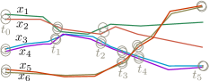
Figure 1: For $m=2$ and $\delta>t_{4}-t_{3}$ there are four maximal groups: $\{x_{1},x_{2}\}$, $\{x_{3},x_{4}\}$, $\{x_{5},x_{6}\}$, and $\{x_{1},..,x_{4}\}$.

We denote the interval $I=[t_{s},t_{e}]$ of group $G$ with $I_{G}$. Group $H$ covers group $G$ if $G\subseteq H$ and $I_{G}\subseteq I_{H}$. If there are no groups that cover $G$, we say $G$ is maximal (on $I_{G}$). In Fig. 1, groups $\{x_{1},x_{2}\}$, $\tilde{G}=\{x_{3},x_{4}\}$, $\hat{G}=\{x_{5},x_{6}\}$, and $G$ $=\{x_{1},..,x_{4}\}$ are maximal: $\tilde{G}$ and $\hat{G}$ on $[t_{0},t_{5}]$, $G$ on $[t_{1},t_{2}]$. Group $\{x_{1},x_{3}\}$ is covered by $G$ and hence not maximal.

Note that entities can be in multiple maximal groups at the same time. For example, entities $\{y_{1},y_{2},y_{3}\}$ can travel together for a while, then $y_{4},y_{5}$ may become $\varepsilon$-connected, and shortly thereafter $y_{1},y_{4},y_{5}$ separate and travel together for a while. Then $y_{1}$ may be in two otherwise disjoint maximal groups for a short time. An entity can also be in two maximal groups where one is a subset of the other. In that case the group with fewer entities must last longer. That an entity is in more groups simultaneously may seem counterintuitive at first, but it is necessary to capture all grouping information. We will show that the total number of maximal groups is $O(\tau n^{3})$, where $n$ is the number of entities in $\mathcal{X}$ and $\tau$ is the number of edges of each input trajectory. This bound is tight in the worst case.

Our maximal group definition uses three parameters, which all allow a more global view of the grouping structure. In particular, we observe that there is monotonicity in the group size and the duration: If $G$ is a group during interval $I$, and we decrease the minimum required group size $m$ or decrease the minimum required duration $\delta$, then $G$ is still a group on time interval $I$. Also, if $G$ is a maximal group on $I$, then it is also a maximal group for a smaller $m$ or smaller $\delta$. For the spatial parameter $\varepsilon$ we observe monotonicity in a slightly different manner: if $G$ is a group for a given $\varepsilon$, then for a larger value of $\varepsilon$ there exists a group $G^{\prime}\supseteq G$. The monotonicity property is important when we want to have a more detailed view of the data: we do not lose maximal groups in a more detailed view. The group may, however, be extended in size and/or duration.

We capture the grouping structure using a Reeb graph of the $\varepsilon$-connected components together with the set of all maximal groups. Parts of the Reeb graph that do not support a maximal group can be omitted. The grouping structure can help us in answering various questions. For example:

What is the largest/longest maximal group at time $t$?

How many entities are currently (not) in any maximal group?

What is the first maximal group that starts/ends after time $t$?

What is the total time that an entity was part of any maximal group?

Which entity has shared maximal groups with the most other entities? Furthermore, the grouping structure can be used to partition the trajectories in independent data sets, to visualize grouping aspects of the trajectories, and to compare grouping across different data sets.

We also discuss robustness of the grouping structure in the following sense. If an entity $x$ leaves a group $G$ and almost immediately returns, we would like to ignore the small interval on which $x$ and $G$ were separate, and just consider $G\cup\{x\}$ as one group. The maximal group definition given above is not robust, but later in the paper we will study an extension that is. Note that robustness requires an additional parameter that captures how short any interruption in a group may last to be ignored.

Results and Organization

We discuss how to represent the grouping structure in Section 2, and prove that there are always $O(\tau n^{3})$ maximal groups, which is tight in the worst case. Here $n$ is the number of trajectories (entities) and $\tau$ the number of edges in each trajectory. We present an algorithm to compute the trajectory grouping structure and all maximal groups in Section 3. This algorithm runs in $O(\tau n^{3}+N)$ time, where $N$ is the total output size. In Section 4 we make our definitions more robust, and extend our algorithms to this case. In Section 5 we evaluate our methods on synthetic and real-world data.

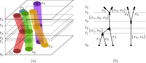
Figure 2: The manifold for the entities $\mathcal{X}=\{x_{1},..,x_{5}\}$ (a), and the corresponding Reeb graph (b).

2 Representing the Grouping Structure

Let $\mathcal{X}$ be a set of $n$ entities, where each entity travels along a path of $\tau$ edges. To compute the grouping structure we consider a manifold $\mathcal{M}$ in $\mathbb{R}^{3}$, where the $z$-axis corresponds to time. The manifold $\mathcal{M}$ is the union of $n$ “tubes” (see Fig. 2(a)). Each tube consists of $\tau$ skewed cylinders with horizontal radius $\varepsilon$ that we obtain by tracing the $\varepsilon$-disc of an entity $x$ over its trajectory.

Let $H_{t}$ denote the horizontal plane at height $t$, then the set $\mathcal{M}\cap H_{t}$ is the level set of $t$. The connected components in the level set of $t$ correspond to the components (maximal sets of $\varepsilon$-connected entities) at time $t$. We will assume for simplicity that all trajectories have their known positions at the same times $t_{0},..,t_{\tau}$ and that no three entities become $\varepsilon$-(dis)connected at the same time, but most of our theory does not depend on these assumptions.

2.1 The Reeb Graph

We start out with a possibly disconnected solid that is the union of a collection of tube-like regions: a 3-manifold with boundary. Note that this manifold is not explicitly defined. We are interested in horizontal cross-sections, and the evolution of the connected components of these cross-sections defines the Reeb graph. Note that this is different from the usual Reeb graph that is obtained from the 2-manifold that is the boundary of our 3-manifold, using the level sets of the height function (the function whose level sets we follow is the height function above a horizontal plane below the manifold), see [4] for a background on these topics.

To describe how the components change over time, we consider the Reeb graph $\mathcal{R}$ of $\mathcal{M}$ (Fig. 2(b)). The Reeb graph has a vertex $v$ at every time $t_{v}$ where the components change. The vertex times are usually not at any of the given times $t_{0},..,t_{\tau}$, but in between two consecutive time steps. The vertices of the Reeb graph can be classified in four groups. There is a start vertex for every component at $t_{0}$ and an end vertex at $t_{\tau}$. A start vertex has in-degree zero and out-degree one, and an end vertex has in-degree one and out-degree zero. The remaining vertices are either merge vertices or split vertices. Since we assume that no three entities become $\varepsilon$-(dis)connected at exactly the same time there are no simultaneous splits and merges. This means merge vertices have in-degree two and out-degree one, and split vertices have in-degree one and out-degree two. A directed edge $e=(u,v)$ connecting vertices $u$ and $v$, with $t_{u}<t_{v}$, corresponds to a set $C_{e}$ of entities that form a component at any time $t\in I_{e}=[t_{u},t_{v}]$. The Reeb graph is this directed graph. Note that the Reeb graph depends on the spatial parameter $\varepsilon$, but not on the other two parameters of maximal groups.

Lemma 2.1

The Reeb graph $\mathcal{R}$ for a set $\mathcal{X}$ of $n$ entities, each of which travels along a trajectory of $\tau$ edges, can have $\Omega(\tau n^{2})$ vertices and $\Omega(\tau n^{2})$ edges.

Proof 2.2

We construct $n$ trajectory edges on which the entities travel in between two consecutive time stamps, say $t_{i}$ and $t_{i+1}$, such that the Reeb graph for $\varepsilon=0$ has $\Omega(n^{2})$ vertices $v$ with $t_{v}\in[t_{i},t_{i+1}]$. We use this construction in between all times $t_{2i}$ and $t_{2i+1}$, and move the entities back to their starting position in between $t_{2i+1}$ and $t_{2i+2}$. Therefore, the total number of vertices is $\Omega(\tau n^{2})$. Since each vertex has degree one or three it follows that the number of edges is also $\Omega(\tau n^{2})$.

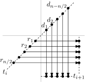
Figure 3: Every pair of entities $r_{j}$ and $d_{\ell}$ are at the same point at time $t_{i}+j+\ell$. This yields $\Omega(n^{2})$ vertices in the interval $[t_{i},t_{i+1}]$.

Let $\mathcal{X}=R\cup D$, with $R=r_{1},..,r_{n/2}$ and $D=d_{1},..,d_{n-n/2}$. At the start (time $t_{i}$) all entities start at the line $y=x$. In particular, we place $r_{j}$ on $(-j,-j)$ and $d_{\ell}$ on $(\ell,\ell)$. All entities move with speed one. The entities in $R$ move to the right, and the entities in $D$ move downwards (see Fig. 3). It follows that each entity $r_{j}$ and $d_{\ell}$ are both at the same point at time $t_{i}+j+\ell$. Hence, we get a vertex in the Reeb graph. There are $\Omega(n^{2})$ such intersections, and thus $\Omega(n^{2})$ vertices. The lemma follows.

Theorem 2.3

Given a set $\mathcal{X}$ of $n$ entities, in which each entity travels along a trajectory of $\tau$ edges, the Reeb graph $\mathcal{R}=(V,E)$ has $O(\tau n^{2})$ vertices and edges. These bounds are tight in the worst case.

Proof 2.4

Lemma 2.1 gives a simple construction that shows that the Reeb graph may have $\Omega(\tau n^{2})$ vertices and edges. For the upper bound, consider a trajectory edge $(v_{i},v_{i+1})$ of (the trajectory of) entity $x\in\mathcal{X}$. An other entity $y\in\mathcal{X}$ is directly connected to $x$ during at most one interval $I\subseteq[t_{i},t_{i+1}]$. This interval yields at most two vertices in $\mathcal{R}$. The trajectory of $x$ consists of $\tau$ edges, hence a pair $x,y$ produces $O(\tau)$ vertices in $\mathcal{R}$. This gives a total of $O(\tau n^{2})$ vertices. Each vertex has constant degree, so there are $O(\tau n^{2})$ edges.

The Trajectory Grouping Structure

The trajectories of entities are associated with the edges of the Reeb graph in a natural way. Each entity follows a directed path in the Reeb graph from a start vertex to an end vertex. Similarly, (maximal) groups follow a directed path from a start or merge vertex to a split or end vertex. If $m>0$ or $\delta>0$, there may be edges in the Reeb graph with which no group is associated. These edges do not contribute to the grouping structure, so we can discard them. The remainder of the Reeb graph we call the reduced Reeb graph, which, together with all maximal groups associated with its edges, forms the trajectory grouping structure.

2.2 Bounding the Number of Maximal Groups

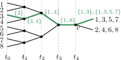
Figure 4: The maximal groups containing entity $3$ (green). Vertex $v$ creates six new groups, including $\{1,3\}$ and $\{1,3,5,7\}$.

To bound the total number of maximal groups, we study the case where $m=1$ and $\delta=0$, because larger values can only reduce the number of maximal groups. It may seem as if each vertex in the Reeb graph simply creates as many maximal groups as it has outgoing edges. However, consider for example Fig. 4. Split vertex $v$ creates not only the maximal groups $\{1,3,5,7\}$ and $\{2,4,6,8\}$, but also $\{1,3\}$, $\{5,7\}$, $\{2,4\}$, and $\{6,8\}$. These last four groups are all maximal on $[t_{2},t]$, for $t>t_{4}$. Notice that all six newly discovered groups start strictly before $t_{v}$, but only at $t_{v}$ do we realize that these groups are maximal, which is the meaning that should be understood with “creating maximal groups”. This example can be extended to arbitrary size. Hence a vertex $v$ may create many new maximal groups, some of which start before $t_{v}$. We continue to show that we may obtain $\Omega(\tau n^{3})$ maximal groups, and that it cannot get worse than that, that is, the number of maximal groups is at most $O(\tau n^{3})$ as well.

Lemma 2.5

For a set $\mathcal{X}$ of $n$ entities, in which each entity travels along a trajectory of $\tau$ edges, there can be $\Omega(n^{3}\tau)$ maximal groups.

Proof 2.6

Similar to Lemma 2.1 we construct $n$ trajectory edges on which the entities travel in between $t_{i}$ and $t_{i+1}$, and repeat this construction in $O(\tau)$ time steps. Our construction yields $\Omega(n^{3})$ maximal groups $G$ with $I_{G}\subseteq[t_{i},t_{i+1}]$, resulting in $\Omega(\tau n^{3})$ maximal groups overall as claimed.

For ease of notation we assume that $n$ is divisible by four, and we write $x$ to denote both the entity $x$ and the $\varepsilon$-disc of entity $x$. We partition our set of entities $\mathcal{X}$ into two sets $S$ and $D$. The entities in $S=\{s_{1},..,s_{3n/4}\}$ are stationary. They all lie on the line $y=0$, ordered from left to right, with a distance $r<2\varepsilon$ in between two consecutive entities. Hence $S$ is $\varepsilon$-connected.

The remaining entities $D$ will move on a horizontal line $y=\nu$, for some $\varepsilon<\nu<2\varepsilon$. At time $t_{i}$, the discs $D=\{d_{1},..,d_{n/4}\}$, ordered from right to left, all lie to the left of the discs in $S$. They all move to the right with the same speed. The distance $h_{i}$ between $d_{i}$ and $d_{i+1}$ is $r+(n/4-i)\mu$, for some small $\mu>0$. Hence, the distances get smaller the further the discs are to the left. See Fig. 5 for an illustration of this construction.

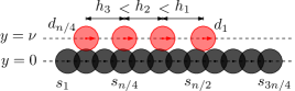
Figure 5: The lower bound construction for $n=16$. The black discs correspond to the stationary entities in $S$. The red (grey) discs correspond the entities in $D$.

We can choose the exact values for $r$ and $\nu$ such that the sequence of events can be partitioned into rounds. Round $i$ consists of a series of $k_{i}$ merge events followed by a series of $k_{i}$ split events. In a series $J_{1},..,J_{k}$ of merges the discs $d_{1},..,d_{k}$ become directly connected with discs in $S$. Merge $J_{i}$ will start a new maximal group $G_{1i}$, where $G_{ij}=S\cup\bigcup_{\ell=i}^{j}d_{\ell}$. Hence after the $k$ merges, $k$ maximal groups have started. In the subsequent series $P_{1},..,P_{k}$ of split events, the discs $d_{1},..,d_{k}$ stop being directly connected with a disc in $S$. When $d_{i}$ leaves, the sets of entities $G_{ii},..,G_{ik}$ end as maximal groups. However, when $d_{i}$ leaves $G_{ij}$, it creates $G_{(i+1)j}$ as a new maximal group that started on $J_{(i+1)}$ (see Fig. 6). This means $P_{i}$ creates $k-i$ new maximal groups.

Figure 6: The time intervals on which $G_{ij}$ is a maximal group in a given round.

We now show that, for any $m\leq 3n/4$ and any $\delta$, this construction yields $\Omega(n^{3})$ maximal groups. Since we can choose the speed of the discs in $D$, we can choose it such that all groups have a minimum duration of at least $\delta$. Now consider the rounds $n/2,..,3n/4$. In each of these rounds we have $k=n/4$ merges followed by $n/4$ splits. The splits in each round create a total of $\sum_{i=1}^{n/4}(n/4-i)=\Omega(n^{2})$ new maximal groups. Each of these groups contains $S$, hence its size is at least $3n/4$. It follows that the total number of maximal groups in those $n/4$ rounds is $\Omega(n^{3})$.

Theorem 2.7

Let $\mathcal{X}$ be a set of $n$ entities, in which each entity travels along a trajectory of $\tau$ edges. There are at most $O(\tau n^{3})$ maximal groups, and this is tight in the worst case.

Proof 2.8

Lemma 2.5 gives a construction that shows that there may be $\Omega(\tau n^{3})$ maximal groups.

We proceed with the upper bound. Every maximal group starts either at a start vertex, or a merge vertex. We will show that the number of maximal groups starting at a start or merge vertex is $O(n)$. Since there are $O(\tau n^{2})$ start and merge vertices the lemma follows. We will discuss only the merge vertex case; the proof for a start vertex is the same.

Let $v$ be a merge vertex, let $S\subset\mathcal{X}$ and $T\subset\mathcal{X}$ be the components that merge at $v$, and let $p_{x}$ denote the path of entity $x\in S\cup T$ through $\mathcal{R}$, starting at $v$. The union over all $x$ of these paths $p_{x}$ forms a directed acyclic graph (DAG) $\mathcal{R}^{\prime}_{v}$, which is a subgraph of $\mathcal{R}$ (see Fig. 7 (a)). Consider “unraveling” $\mathcal{R}^{\prime}_{v}$ into a tree $\mathcal{T}_{v}$ as follows. If $p_{x}$ and $p_{y}$ split in some vertex $u$ and merge again in vertex $w$, with $t_{w}>t_{u}$ we duplicate the subpath starting at $w$. This yields a tree $\mathcal{T}_{v}$ with root $v$ and at most $|S|+|T|\leq n$ leaves. Furthermore, all nodes in $\mathcal{T}_{v}$ have degree at most three (see Fig. 7 (b)).

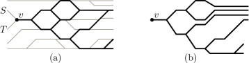
Figure 7: DAG $\mathcal{R}^{\prime}_{v}$ (black) as a subgraph of $\mathcal{R}$ (grey) (a), and the tree $\mathcal{T}_{v}$ obtained by unfolding $\mathcal{R}^{\prime}_{v}$ (b).

Since all maximal groups end at either a split or an end vertex, all maximal groups $G_{1},..,G_{k}$ that start at $v$ can now be represented by subpaths in $\mathcal{T}_{v}$ starting at the root. The path corresponding to a maximal group $G$ ends at the first node where two entities $x,y\in G$ split, or at a leaf if no such node exists. Clearly, paths $p_{x}$ and $p_{y}$ can split only at a degree three node. Since $\mathcal{T}_{v}$ has at most $n$ leaves it follows there are at most $O(n)$ degree three nodes.

Finally, we show that there is at most one maximal group that ends at a given leaf or degree three node of $\mathcal{T}_{v}$. Assume by contradiction that $G_{i}$ and $G_{j}$, with $i\neq j$, both end at node $u$. Both maximal groups share the same path from the root of $\mathcal{T}_{v}$ to $u$, so all entities in $G_{i}$ and $G_{j}$ are in the same component at all times $t\in I=[t_{v},t_{u}]$. Hence $G_{i}\cup G_{j}$ is a maximal group on $I$, contradicting that $G_{i}$ and $G_{j}$ were maximal. We conclude that the number of maximal groups $k$ that start at $v$ is at most the number of leaves plus the number of degree three nodes in $\mathcal{T}_{v}$. Hence $k=O(n)$. Summing over all $O(\tau n^{2})$ start and merge vertices gives $O(\tau n^{3})$ maximal groups in total.

3 Computing the Grouping Structure

To compute the grouping structure we need to compute the reduced Reeb graph and the maximal groups. We now show how to do this efficiently. Removing the edges of the Reeb graph that are not used is an easy post-processing step which we do not discuss further.

3.1 Computing the Reeb Graph

We can compute the Reeb graph $\mathcal{R}=(V,E)$ as follows. We first compute all times where two entities $x$ and $y$ are at distance $2\varepsilon$ from each other. We distinguish two types of events, connect events at which $x$ and $y$ become directly connected, and disconnect events at which $x$ and $y$ stop being directly connected.

We now process the events on increasing time while maintaining the current components. We do this by maintaining a graph $G=(\mathcal{X},Z)$ representing the directly-connected relation, and the connected components in this graph. The set of vertices in $G$ is the set of entities. The graph $G$ changes over time: at connect events we insert new edges into $G$, and at disconnect events we remove edges.

At any given time $t$, $G$ contains an edge $(x,y)$ if and only if $x$ and $y$ are directly connected at time $t$. Hence the components at $t$ (the maximal sets of $\varepsilon$-connected entities) correspond to the connected components in $G$ at time $t$. Since we know all times at which $G$ changes in advance, we can use the same approach as Parsa [18] to maintain the connected components: we assign a weight to each edge in $G$ and we represent the connected components using a maximum weight spanning forest. The weight of edge $(x,y)$ is equal to the time at which we remove it from $G$, that is, the time at which $x$ and $y$ become directly disconnected. We store the maximum weight spanning forest $F$ as an ST-tree [19], which allows connectivity queries, inserts, and deletes, in $O(\log n)$ time.

We spend $O(n^{2})$ time to initialize the graph $G$ at $t_{0}$ in a brute-force manner. For each component we create a start vertex in $\mathcal{R}$. We also initialize a one-to-one mapping $M$ from the current components in $G$ to the corresponding vertices in $\mathcal{R}$. When we handle a connect event of entities $x$ and $y$ at time $t$, we query $F$ to get the components $C_{x}$ and $C_{y}$ containing $x$ and $y$, respectively. Using $M$ we locate the corresponding vertices $v_{x}$ and $v_{y}$ in $\mathcal{R}$. If $C_{x}\neq C_{y}$ we create a new merge vertex $v$ in $\mathcal{R}$ with time $t_{v}=t$, add edges $(v_{x},v)$ and $(v_{y},v)$ to $\mathcal{R}$ labeled $C_{x}$ and $C_{y}$, respectively. If $C_{x}=C_{y}$ we do not change $\mathcal{R}$. Finally, we add the edge $(x,y)$ to $G$ (which may cause an update to $F$), and update the mapping $M$.

At a disconnect event we first query $F$ to find the component $C$ currently containing $x$ and $y$. Using $M$ we locate the vertex $u$ corresponding to $C$. Next, we delete the edge $(x,y)$ from $G$, and again query $F$. Let $C_{x}$ and $C_{y}$ denote the components containing $x$ and $y$, respectively. If $C_{x}=C_{y}$ we are done, meaning $x$ and $y$ are still $\varepsilon$-connected. Otherwise we add a new split vertex $v$ to $\mathcal{R}$ with time $t_{v}=t$, and an edge $e=(u,v)$ with $C_{e}=C$ as its component. We update $M$ accordingly.

Finally, we add an end vertex $v$ for each component $C$ in $F$ with $t_{v}=t_{\tau}$. We connect the vertex $u=M(C)$ to $v$ by an edge $e=(u,v)$ and let $C_{e}=C$ be its component.

Analysis

We need $O(\tau n^{2}\log n)$ time to compute all $O(\tau n^{2})$ events and sort them according to increasing time. To handle an event we query $F$ a constant number of times, and we insert or delete an edge in $F$. These operations all take $O(\log n)$ time. So the total time required for building $\mathcal{R}$ is $O(\tau n^{2}\log n)$.

Theorem 3.1

Given a set $\mathcal{X}$ of $n$ entities, in which each entity travels along a trajectory of $\tau$ edges, the Reeb graph $\mathcal{R}=(V,E)$ has $O(\tau n^{2})$ vertices and edges, and can be computed in $O(\tau n^{2}\log n)$ time.

3.2 Computing the Maximal Groups

We now show how to compute all maximal groups using the Reeb graph $\mathcal{R}=(V,E)$. We will ignore the requirements that each maximal group should contain at least $m$ entities and have a minimal duration of $\delta$. That is, we assume $m=1$ and $\delta=0$. It is easy to adapt the algorithm for larger values.

Labeling the Edges

Our algorithm labels each edge $e=(u,v)$ in the Reeb graph with a set of maximal groups $\mathcal{G}_{e}$. The groups $G\in\mathcal{G}_{e}$ are those groups for which we have discovered that $G$ is a maximal group at a time $t\leq t_{u}$. Each maximal group $G$ becomes maximal at a vertex, either because a merge vertex created $G$ as a new group that is maximal, or because $G$ is now a maximal set of entities that is still together after a split vertex. This means we can compute all maximal groups as follows.

We traverse the set of vertices of $\mathcal{R}$ in topological order. For every vertex $v$ we compute the maximal groups on its outgoing edge(s) using the information on its incoming edge(s).

If $v$ is a start vertex it has one outgoing edge $e=(v,u)$. We set $\mathcal{G}_{e}$ to $\{(C_{e},t_{v})\}$ where $t_{v}=t_{0}$. If $v$ is a merge vertex it has two incoming edges, $e_{1}$ and $e_{2}$. We propagate the maximal groups from $e_{1}$ and $e_{2}$ on to the outgoing edge $e$, and we discover $(C_{e},t_{v})$ as a new maximal group. Hence $\mathcal{G}_{e}=\mathcal{G}_{e_{1}}\cup\mathcal{G}_{e_{2}}\cup\{(C_{e},t_{v})\}$.

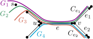
Figure 8: After split vertex $v$, $\mathcal{G}_{e_{1}}$ contains the groups $C_{e_{1}}=G_{1}\cup G_{2}$ (with starting time $t_{s}$), $G_{1}$, and $G_{2}$. Maximal groups $C_{e_{2}}=G_{3}\cup G_{4}$ (with starting time $t_{u}$), $G_{3}$, and $G_{4}$ go to $e_{2}$. The maximal groups $C_{e}$ and $G_{1}\cup G_{2}\cup G_{3}$ end at $v$.

If $v$ is a split vertex it has one incoming edge $e$, and two outgoing edges $e_{1}$ and $e_{2}$. A maximal group $G$ on $e$ may end at $v$, continue on $e_{1}$ or $e_{2}$, or spawn a new maximal group $G^{\prime}\subset G$ on either $e_{1}$ or $e_{2}$. In particular, for any group $G^{\prime}$ in $\mathcal{G}_{e_{i}}$, there is a group $G$ in $\mathcal{G}_{e}$ such that $G^{\prime}=G\cap C_{i}\neq\emptyset$. The starting time of $G^{\prime}$ is $t^{\prime}=\min\{t\mid(G,t)\in\mathcal{G}_{e}\land G^{\prime}\subseteq G\}$. Thus, $t^{\prime}$ is the first time $G^{\prime}$ was part of a maximal group on $e$. Stated differently, $t^{\prime}$ is the first time $G^{\prime}$ was in a component on a path to $v$. Fig. 8 illustrates this case. If $v$ is an end vertex it has no outgoing edges. So there is nothing to be done.

Fig. 9 shows a complete example of a Reeb graph after labeling the edges with their maximal groups.

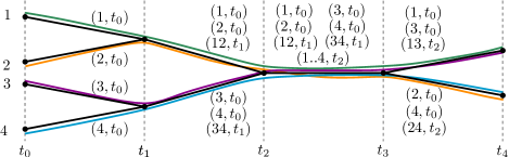
Figure 9: The maximal groups as computed by our algorithm (a set $\{i,j,k\}$ is denoted by $ijk$).

Storing the Maximal Groups

We need a way to store the maximal groups $\mathcal{G}_{e}$ on an edge $e=(u,v)$ in such a way that we can efficiently compute the set(s) of maximal groups on the outgoing edge(s) of a vertex $v$. We now show that we can use a tree $\mathcal{T}_{e}$ to represent $\mathcal{G}_{e}$, with which we can handle a merge vertex in $O(1)$ time, and a split vertex in $O(k)$ time, where $k$ is the number of entities involved. The tree uses $O(k)$ storage.

We say a group $G$ is a subgroup of a group $H$ if and only if $G\subseteq H$ and $I_{H}\subseteq I_{G}$. For example, in Fig. 1 $\{x_{1},x_{2}\}$ is a subgroup of $\{x_{1},..,x_{4}\}$. Note that both $G$ and $H$ could be maximal.

Lemma 3.2

Let $e$ be an edge of $\mathcal{R}$, and let $S$ and $T$ be maximal groups in $\mathcal{G}_{e}$ with starting times $t_{S}$ and $t_{T}$, respectively. There is also a maximal group $G\supseteq S\cup T$ on $e$ with starting time $t_{G}\geq\max(t_{S},t_{T})$, and if $S\cap T\neq\emptyset$ then $S$ is a subgroup of $T$ or vice versa.

Proof 3.3

The first statement is almost trivial. Clearly, $S,T\subseteq C_{e}$ and hence $S\cup T\subseteq C_{e}$. Component $C_{e}$ itself is also a maximal group on $e$. By construction $C_{e}$ must have the largest starting time $t$ of the groups in $\mathcal{G}_{e}$. Hence $t_{G}\geq\max(t_{S},t_{T})$.

We prove the second statement by contradiction: assume $S\cap T\neq\emptyset$, and $S\not\subseteq T$ or vice versa. Assume w.l.o.g. that $t_{S}\leq t_{T}$. So the entities in $S$ are all in a single component at all times $t\geq t_{T}\geq t_{S}$. At any time $t\geq t_{T}$ all entities in $T$ are also in a single component. Since $S\cap T\neq\emptyset$ this must be the same component that contains $S$. Hence $S\subseteq T$, which together with $t_{S}\leq t_{T}$ proves the statement.

We represent the groups $\mathcal{G}_{e}$ on an edge $e\in E$ by a tree $\mathcal{T}_{e}$ (see Fig. 10). We call this the grouping tree. Each node $v$ represents a group $G_{v}\in\mathcal{G}_{e}$. The children of a node $v$ are the largest subgroups of $G_{v}$. From Lemma 3.2 it follows that any two children of $v$ are disjoint. Hence an entity $x\in G_{v}$ occurs in only one child of $v$. Furthermore, note that the starting times are monotonically decreasing on the path from the root to a leaf: smaller groups started earlier. A leaf corresponds to a smallest maximal group on $e$: a singleton set with an entity $x\in C_{e}$. It follows that $\mathcal{T}_{e}$ has $O(n)$ leaves, and therefore has size $O(n)$. Note, however, that the summed sizes of all maximal groups can be quadratic.

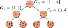
Figure 10: The grouping tree for the edge between $t_{2}$ and $t_{3}$ in Fig. 9.

Analysis

We analyze the time required to label each edge $e$ with a tree $\mathcal{T}_{e}$ for a given Reeb graph $\mathcal{R}=(V,E)$. Topologically sorting the vertices takes linear time. So the running time is determined by the processing time in each vertex, that is, computing the tree(s) $\mathcal{T}_{e}$ on the outgoing edge(s) $e$ of each vertex. Start, end, and merge vertices can be handled in $O(1)$ time: start and end vertices are trivial, and at a merge vertex $v$ the tree $\mathcal{T}_{e}$ is simply a new root node with time $t_{v}$ and as children the (roots of the) trees of the incoming edges. At a split vertex we have to split the tree $\mathcal{T}=\mathcal{T}_{(u,v)}$ of the incoming edge $(u,v)$ into two trees for the outgoing edges of $v$. For this, we traverse $\mathcal{T}$ in a bottom-up fashion, and for each node, check whether it induces a vertex in one or both of the trees after splitting. This algorithm runs in $O(|\mathcal{T}|)$ time. Since $|\mathcal{T}|=O(n)$ the total running time of our algorithm is $O(n|V|)=O(\tau n^{3})$.

Reporting the Groups

We can augment our algorithm to report all maximal groups at split and end vertices. The main observation is that a maximal group ending at a split vertex $v$, corresponds exactly to a node in the tree $\mathcal{T}_{(u,v)}$ (before the split) that has entities in leaves below it that separate at $v$. The procedures for handling split and end vertices can easily be extended to report the maximal groups of size at least $m$ and duration at least $\delta$ by simply checking this for each maximal group. Although the number of maximal groups is $O(\tau n^{3})$ (Theorem 2.7), the summed size of all maximal groups can be $\Omega(\tau n^{4})$. The running time of our algorithm is $O(\tau n^{3}+N)$, where $N$ is the total output size.

Theorem 3.4

Given a set $\mathcal{X}$ of $n$ entities, in which each entity travels along a trajectory of $\tau$ edges, we can compute all maximal groups in $O(\tau n^{3}+N)$ time, where $N$ is the output size.

4 Robustness

The grouping structure definition we have given and analyzed has a number of good properties. It fulfills monotonicity, and in the previous sections we showed that there are only polynomially many maximal groups, which can be computed in polynomial time as well. In this section we study the property of robustness, which our definition of grouping structure does not have yet. Intuitively, a robust grouping structure ignores short interruptions of groups, as these interruptions may be insignificant at the temporal scale at which we are studying the data. For example, if we are interested in groups that have a duration of one hour or more, we may want to consider interruptions of a minute or less insignificant.

We introduce a new temporal parameter $\alpha$, which is related to the temporal scale at which the data is studied. Our robust grouping structure should ignore interruptions of duration at most $\alpha$. We realize this by letting the precise moment of events be irrelevant beyond a value depending on $\alpha$. Events that happen within $\alpha$ time of each other may cancel out, or their order may be exchanged. The objective is to incorporate $\alpha$ into our definitions while maintaining the properties that we have for the (non-robust) grouping structure. Note that $\alpha$ is another parameter that allows us to obtain more generalized views of the grouping structure by increasing its value. Obtaining generalized views in this way is related to the concept of persistence in computational topology [4, 5].

A possible definition of a robust grouping structure is based on the following intuition: A set of entities forms a robust group on $I$ as long as every interval $I^{\prime}\subset I$ on which its entities are not in the same component has length at most $\alpha$. More formally: we say $G$ is a robust group on time interval $I$ if and only if: (i) $G$ contains at least $m$ entities, (ii) $I$ has length at least $\delta$, and (iii) for any time $t\in I$ there is a time $t^{\prime}\in[t-\alpha/2,\;t+\alpha/2]$ and a component $C\in\mathcal{C}(t^{\prime})$ such that $G\subseteq C$. Unfortunately, we can show that even determining whether there is a robust group of size $k$ is NP-complete (see Appendix A).

We consider a second definition for a robust group, which we will use from now on. Two entities are $\alpha$-relaxed directly connected at time $t$ if and only if they are directly connected at some time $t^{\prime}\in[t-\alpha/2,\;t+\alpha/2]$. Two entities $x$ and $y$ are $\alpha$-relaxed $\varepsilon$-connected at time $t$ if there is a sequence $x=x_{0},..,x_{j}=y$ such that $x_{i}$ and $x_{i+1}$ are $\alpha$-relaxed directly connected. Note that the precise times may be different for different pairs $x_{i}$ and $x_{i+1}$, as long as each time is in the interval $[t-\alpha/2,\;t+\alpha/2]$. A maximal set of $\alpha$-relaxed $\varepsilon$-connected entities at time $t$ is an $\alpha$-relaxed component, or $\alpha$-component for short. An $\alpha$-component at time $t$ corresponds to connected $3D$-component in a horizontal slice of $\mathcal{M}$ with thickness $\alpha$ and centered at $t$ (see Fig. 11).

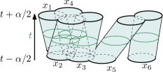
Figure 11: An $\alpha$-component at time $t$.

A subset $G$ of $k$ entities is a robust group if and only if it is a group by the definition in the introduction, but where “component” is replaced by “$\alpha$-component” in condition (iii). This immediately leads to the definition of maximal robust groups and a robust grouping structure. The robust grouping structure has the property of monotonicity in the new parameter $\alpha$ as well. Note that every group which is a robust group according to the first definition, is also a robust group according to the second definition. For instance, in Fig. 11, entities $x_{1},..,x_{6}$ form a component by the second definition, but not by the first.

4.1 Computation of Maximal Robust Groups

We can compute all maximal robust groups according to the (second) definition. The idea is to modify the Reeb graph to a version that is parametrized by $\alpha$ and captures exactly the robust grouping structure for parameter $\alpha$.

Let $\mathcal{R}$ be the Reeb graph that we used for the grouping structure without considering robustness. Note that this is the same as assuming $\alpha=0$ in the definition of the robust grouping structure, and we let $\mathcal{R}_{0}=\mathcal{R}$. For $\alpha>0$ we define the Reeb graph parametrized in $\gamma$ as $\mathcal{R}_{\gamma}$ by imagining a process that changes the Reeb graph for a growing parameter $\gamma$, starting with $\mathcal{R}_{0}$ and ending with $\mathcal{R}_{\alpha/2}$.

We observe that a new $\alpha$-component starts at time $\alpha/2$ before two regular components merge and form a new component. Symmetrically, an $\alpha$-component ends due to a split at time $\alpha/2$ after a regular component splits. Both facts follow from the new definition of $\alpha$-relaxed directly connected. It implies that in the process that maintains $\mathcal{R}_{\gamma}$ for growing $\gamma$, the split nodes move forward in time, zippering together the outgoing edges, and the merge nodes move backward in time, zippering together the incoming edges. All nodes move at the same rate in $\gamma$, which implies that in the process, the only event where the Reeb graph changes structurally is when an (earlier) split node encounters a (later) merge node. This can happen only if they are endpoints of the same edge of the Reeb graph. The encounter is either a passing or a collapse (see Fig. 12).

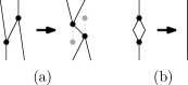
Figure 12: Passing encounter, before and after (a). Collapse encounter, before and after (b).

Both encounters lead to new edges in the Reeb graph and can thus give rise to new encounters when growing $\gamma$ further. The collapse encounter reduces the complexity of the Reeb graph: two nodes of degree $3$ disappear and four edges become a single edge. The collapse event is exactly the situation where a component splits and merges again, so by removing a split-merge pair involving the same entities we ignore the temporary split of a component (or group).

A passing encounter maintains the complexity of the Reeb graph. Before the passing encounter, a part of one group splits and merges with a different group. After the passing encounter, the two groups merge (for a short time) and then split again. This situation is also captured in Fig. 11.

Next, we show that there are $O(\tau n^{3})$ encounter events in the Reeb graph of the robust version of the trajectory grouping structure, and this bound is tight in the worst case.

Lemma 4.1

For some set $\mathcal{X}$ of $n$ entities, in which each entity travels along a trajectory of $\tau$ edges, the structure of the Reeb graph $\mathcal{R}_{\gamma}$ of $\mathcal{X}$ changes $\Omega(\tau n^{3})$ times when increasing $\gamma$ from zero to infinity.

Proof 4.2

We show that there is a set of $n$ trajectories, each consisting of $\tau$ edges, for which there are $\Omega(\tau n^{3})$ encounter events. The lemma then follows.

We use the same construction as in Lemma 2.5. So in all time intervals $[t_{2i},t_{2i+1}]$ we have a set $S$ of $3n/4$ stationary entities/discs and a set $D=\{d_{1},..,d_{n/4}\}$ entities, ordered from right to left, that move to the right in such a way that $d_{i}$ becomes directly (dis)connected with $S$ before $d_{i+1}$ (see Fig. 5). Let $t_{a}$ be the first time at which $d_{n/4}$ becomes directly connected with $S$, and let $t_{b}$ denote the last time $d_{1}$ becomes directly disconnected with $S$. We now show that the part of Reeb-graph $\mathcal{R}^{\prime}$ corresponding to the interval $(t_{a},t_{b})$ already yields $\Omega(n^{3})$ encounter events. We note that no other encounter events involving other parts of the Reeb-graph can interfere with the encounter events in $\mathcal{R}^{\prime}$.

In between $t_{a}$ and $t_{b}$ every disc $d_{i}$ becomes directly (dis)connected with $S$ $\Omega(n)$ times. So $\mathcal{R}^{\prime}_{\gamma}$ initially contains of a path $P$ of $\Omega(n^{2})$ edges. Each edge has at least the set of entities $S$ associated with it, and possibly other entities as well. The vertices on $P$ can be grouped in $\Omega(n)$ sequences of $k=n/4$ split vertices $u_{1},..,u_{k}$ followed by $k$ merge vertices $v_{1},..,v_{k}$. At vertex $u_{i}$ entity $x_{i}$ splits from $S$ and at $v_{i}$ entity $x_{i}$ merges with $S$. See Fig. 13.

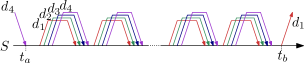
Figure 13: The part of the Reeb-graph that yields $\Omega(n^{3})$ encounter events (for $n=16$).

By increasing $\gamma$ each split vertex $u_{i}$ will have a passing encounter with the merge vertices $v_{1},..,v_{i-1}$ before it collapses with $v_{i}$. Hence each sequence involves $\sum_{i=1}^{k}(i-1)=\Omega(n^{2})$ encounter events. Since there are $\Omega(n)$ such sequences this gives $\Omega(n^{3})$ encounter events in a single timestep, and hence $\Omega(\tau n^{3})$ in total.

Theorem 4.3

Let $\mathcal{X}$ be a set of $n$ entities, in which each entity travels along a trajectory of $\tau$ edges. The structure of the Reeb graph $\mathcal{R}_{\gamma}$ of $\mathcal{X}$ changes at most $O(\tau n^{3})$ times when increasing $\gamma$ from zero to infinity. This bound is tight in the worst case.

Proof 4.4

Lemma 4.1 gives a construction that shows that there may be $\Omega(\tau n^{3})$ encounters.

Since each collapse event decreases the number of edges by three it follows the number of collapse events is at most $O(\tau n^{2})$. What remains is to prove that the number of passing events is $O(\tau n^{3})$. Each passing event involves a split vertex $u$ and a merge vertex $v$. We now show that there are at most $n$ passing events involving a given split vertex $u$. Since there are $O(\tau n^{2})$ split vertices this means the number of passing events is $O(\tau n^{3})$.

Assume by contradiction that there are $k>n$ passing events involving split vertex $u$. Let $\gamma_{1},..,\gamma_{k}$ be the values for $\gamma$ for which these passing events occur in non-decreasing order, and let $v_{1},..,v_{k}$ be the corresponding merge vertices. Just before $u$ passes $v_{i}$ the edge $e=(u,v_{i})$ is an incoming edge of $v_{i}$. Let $X_{i}$ denote the set of entities on the other incoming edge of $v_{i}$, that is the set of entities that merges with $C_{e}$ at vertex $v_{i}$ (see Fig. 14(a)).

Since $k>n$ there must be an entity $x$ that $u$ “passes” at least twice. That is, $u$ passes $v_{i}$ and $v_{j}$, with $i<j$, and $x\in X_{i}$ and $x\in X_{j}$. Now consider the Reeb-graph $\mathcal{R}_{\gamma}$ just after $u$ passes $v_{i}$ (which means $\gamma>\gamma_{i}$). Since $u$ still has to pass $v_{j}$ there is a path $Q$ connecting $u$ to $v_{j}$. By further increasing $\gamma$ this path will eventually become a single edge $(u,v_{j})$, which will flip to $(v_{j},u)$ when $u$ passes $v_{j}$ at $\gamma=\gamma_{j}$.

Entity $x$ is present at the first vertex of $Q$ (vertex $u$), and it merges again with path $Q$ at $v_{j}$. Clearly, this means that $Q$ contains a split vertex $w$ at which $x$ splits from path $Q$ before it can return to $Q$ in vertex $v_{j}$ (see Fig. 14 (b)).

Figure 14: The part of $\mathcal{R}_{\gamma}$ before $u$ encounters $v_{i}$. The set $X_{i}$ merges with $C_{e}$ at vertex $v_{i}$ (a). If $x$ merges at both $v_{i}$ and $v_{j}$ it has to leave (split) at a vertex $w$ in between (b).

We now have two paths connecting $w$ to $v_{j}$: the path that $x$ follows and the subpath of $Q$. We again have that by increasing $\gamma$ both paths will become singleton edges connecting $w$ to $v_{j}$. Eventually both these edges are removed in a collapse event for some $\hat{\gamma}$. If $w=u$ this means $(u,v_{j})$ is actually a collapse event instead of a passing event. Contradiction. If $w\neq u$ we have that $t_{w}>t_{u}$, and therefore $\hat{\gamma}<\gamma_{j}$. The collapse event at $\hat{\gamma}$ will consume both $w$ and $v_{j}$, which means $u$ can no longer pass $v_{j}$. Contradiction. Since both cases yield a contradiction we conclude that the number of passing events involving $u$ is at most $n$. With $O(\tau n^{2})$ vertices this yields the desired bound of $O(\tau n^{3})$ passing events.

Algorithmically, we start with the Reeb graph $\mathcal{R}_{0}$ and examine each edge. Any edge that leads from a split node to a merge node and whose duration is at most $\alpha$ is inserted in a priority queue, where the duration of the edge is the priority. We handle the encounter events in the correct order, changing the Reeb graph and possibly inserting new encounter events in the priority queue. Each event is handled in $O(\log n)$ time since it involves at most $O(1)$ priority queue operations. Since there are $O(\tau n^{3})$ events (Theorem 4.3) this takes $O(\tau n^{3}\log n)$ time in total. Once we have the Reeb graph $\mathcal{R}_{\alpha/2}$, we can associate the trajectories with its edges as before. The computation of the maximal robust groups is done in the same way as computing the maximal groups on the normal Reeb graph $\mathcal{R}$. We conclude:

Theorem 4.5

Given a set $\mathcal{X}$ of $n$ entities, in which each entity travels along a trajectory of $\tau$ edges, we can compute all robust maximal groups in $O(\tau n^{3}\log n+N)$ time, where $N$ is the output size.

5 Evaluation

To see if our model of the grouping structure is practical and indeed captures the grouping behavior of entities we implemented and evaluated our algorithms. We would like to visually inspect the maximal groups identified by our algorithm, and compare this to our intuition of groups. For a small number of (short) trajectories we can still show this in a figure, see for example Fig. 15, which shows the monotonicity of the maximal groups in size and duration. However, for a larger number of trajectories the resulting figures become too cluttered to analyze. So instead we generated short videos.

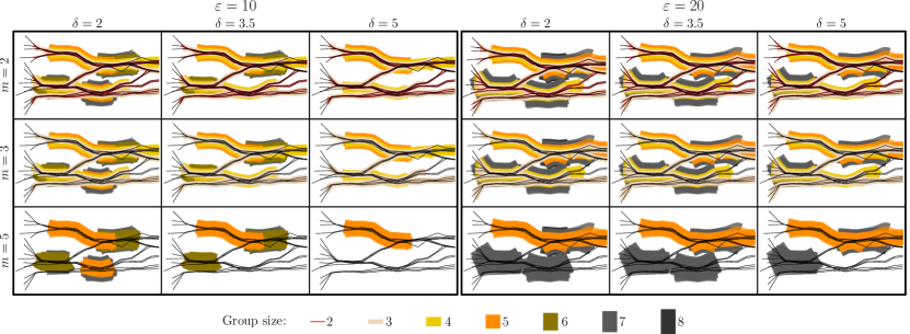
Figure 15: The maximal groups for varying parameter values. The time associated with each trajectory vertex is proportional to its $x$-coordinate.

We use two types of data sets to evaluate our method: a synthetic data set generated using a slightly modified version of the NetLogo Flocking model [23, 24], and a real-world data set consisting of deer, elk, and cattle, tracked in the Starkey project [17].

NetLogo

We generated several data sets using an adapted version of the NetLogo Flocking model [23]. In our adapted model the entities no longer wrap around the world border, but instead start to turn when they approach the border. Furthermore, we allow small random direction changes for the entities. The data set that we consider here contains 400 trajectories, with 818 edges each. Similar to Fig. 15, our videos show all maximal groups for varying parameter values.

The videos show that our model indeed captures the crucial properties of grouping behavior well. We notice that the choice of parameter values is important. In particular, if we make $\varepsilon$ too large we see that the entities are loosely coupled, and too many groups are found. Similarly, for large values of $m$ virtually no groups are found. However, for reasonable parameter settings, for example $\varepsilon=5.25$, $m=4$, and $\delta=100$, we can clearly see that our algorithm identified virtually all sets of entities that travel together. Furthermore, if we see a set of entities traveling together that is not identified as group, we indeed see that they disperse quickly after they have come together. The coloring of the line-segments also nicely shows how smaller groups merge into larger ones, and how the larger groups break up into smaller subgroups. This is further evidence that our model captures the grouping behavior well.

Starkey

We also ran our algorithms on a real-world data set, namely on tracking data obtained in the Starkey project [17]. This data set captures the movement of deer, elk, and cattle in Starkey, a large forest area in Oregon (US), over three years. Not all animals are tracked during the entire period, and positions are not reported synchronously for all entities. Thus, we consider only a subset of the data, and resample the data such that all trajectories have vertices at the same (regularly spaced) times. We chose a period of 30 days for which we have the locations of most of the animals. This yields a data set containing 126 trajectories with 1264 vertices each. In the Starkey video we can see that a large group of entities quickly forms in the center, and then slowly splits into multiple smaller groups. We notice that some entities (groups) move closely together, whereas others often stay stationary, or travel separately.

Running Times

Since we are mainly interested in how well our model captures the grouping behavior, we do not extensively evaluate the running times of our algorithms. On our desktop system with a AMD Phenom II X2 CPU running at 3.2Ghz our algorithm, implemented in Haskell, computes the grouping structure for our data sets in a few seconds. Even for 160 trajectories with roughly 20 thousand vertices each we can compute and report all maximal groups in three minutes. Most of the time is spent on computing the Reeb graph, in particular on computing the connect/disconnect events. Since our implementation uses a slightly easier, yet slower, data structure to represent the maximum weight spanning forest during the construction of the Reeb graph, we expect that some speedup is still possible.

6 Concluding Remarks

We introduced a trajectory grouping structure which uses Reeb graphs and a notion of persistence for robustness. We showed how to characterize and efficiently compute the maximal groups and group changes in a set of trajectories, and bounded their maximal number. Our paper demonstrates that computational topology provides a mathematically sound way to define grouping of moving entities. The complexity bounds, algorithms and implementation together form the first comprehensive study of grouping. Our videos show that our methods produce results that correspond to human intuition.

Further work includes more extensive experiments together with domain specialists, such as behavioral biologists, to ensure further that the grouping structure captures groups and events in a natural, expected way, and changes in the parameters have the desired effect. At the same time, our research may be linked to behavioral models of collective motion [20] and provide a (quantifiable) comparison of these.

We expect that for realistic inputs the size of the grouping structure is much smaller than the worst-case bound that we proved. We plan to confirm this in experiments, and to provide faster algorithms under realistic input models. We will also work on improving the visualization of the maximal groups and the grouping structure, based on the reduced Reeb graph.

Videos accompanying this paper can be found on www.staff.science.uu.nl/~staal006/grouping.

Appendix A NP-completeness of robust grouping by the first definition

Theorem A.1

Determining whether there is a robust group of size $k$ is NP-complete using the first definition of robust groups.

Proof A.2

We prove this by a reduction from

References

- Benkert et al. [2008] M. Benkert, J. Gudmundsson, F. Hübner, and T. Wolle. Reporting flock patterns. Computational Geometry, 41(3):111 – 125, 2008.
- Biasotti et al. [2008] S. Biasotti, D. Giorgi, M. Spagnuolo, and B. Falcidieno. Reeb graphs for shape analysis and applications. Theor. Comput. Sci., 392(1-3):5–22, 2008.
- Dey and Wang [2011] T. K. Dey and Y. Wang. Reeb graphs: approximation and persistence. In Proc. 27th ACM Symposium on Computational Geometry, SoCG ’11, pages 226–235, 2011.
- Edelsbrunner and Harer [2010] H. Edelsbrunner and J. L. Harer. Computational Topology – an introduction. American Mathematical Society, 2010.
- Edelsbrunner et al. [2002] H. Edelsbrunner, D. Letscher, and A. Zomorodian. Topological persistence and simplification. Discrete & Computational Geometry, 28:511–533, 2002.
- Edelsbrunner et al. [2008] H. Edelsbrunner, J. Harer, A. Mascarenhas, V. Pascucci, and J. Snoeyink. Time-varying Reeb graphs for continuous space-time data. Computational Geometry, 41(3):149–166, 2008.
- Ester et al. [1996] M. Ester, H. Kriegel, J. Sander, and X. Xu. A density-based algorithm for discovering clusters in large spatial databases with noise. In Proc. 2nd International Conference on Knowledge Discovery and Data mining, volume 1996, pages 226–231. AAAI Press, 1996.
- Fomenko and Kunii [1997] A. Fomenko and T. Kunii, editors. Topological Methods for Visualization. Springer, Tokyo, Japan, 1997.
- Ge et al. [2011] X. Ge, I. Safa, M. Belkin, and Y. Wang. Data skeletonization via Reeb graphs. In Proc. 25th Annual Conference on Neural Information Processing Systems, NIPS ’11, pages 837–845, 2011.
- Gudmundsson and van Kreveld [2006] J. Gudmundsson and M. van Kreveld. Computing longest duration flocks in trajectory data. In Proc. 14th ACM International Symposium on Advances in Geographic Information Systems, GIS ’06, pages 35–42. ACM, 2006.
- Gudmundsson et al. [2007] J. Gudmundsson, M. van Kreveld, and B. Speckmann. Efficient detection of patterns in 2d trajectories of moving points. GeoInformatica, 11:195–215, 2007.
- Huang et al. [2008] Y. Huang, C. Chen, and P. Dong. Modeling herds and their evolvements from trajectory data. In Geographic Information Science, volume 5266 of LNCS, pages 90–105. Springer, 2008.
- Hwang et al. [2005] S.-Y. Hwang, Y.-H. Liu, J.-K. Chiu, and E.-P. Lim. Mining mobile group patterns: A trajectory-based approach. In Advances in Knowledge Discovery and Data Mining, volume 3518 of LNCS, pages 145–146. Springer, 2005.
- Jeung et al. [2008] H. Jeung, M. L. Yiu, X. Zhou, C. S. Jensen, and H. T. Shen. Discovery of convoys in trajectory databases. PVLDB, 1:1068–1080, 2008.
- Kalnis et al. [2005] P. Kalnis, N. Mamoulis, and S. Bakiras. On discovering moving clusters in spatio-temporal data. In Advances in Spatial and Temporal Databases, volume 3633 of LNCS, pages 364–381. Springer, 2005.
- Li et al. [2010] Z. Li, B. Ding, J. Han, and R. Kays. Swarm: Mining relaxed temporal moving object clusters. PVLDB, 3(1):723–734, 2010.
- Oregon Department of Fish and Wildlife and the USDA Forest Service [2004] Oregon Department of Fish and Wildlife and the USDA Forest Service. The Starkey project, 2004. URL http://www.fs.fed.us/pnw/starkey.
- Parsa [2012] S. Parsa. A deterministic time algorithm for the Reeb graph. In Proc. 28th ACM Symposium on Computational Geometry, pages 269–276, 2012.
- Sleator and Tarjan [1983] D. D. Sleator and R. E. Tarjan. A data structure for dynamic trees. Journal of Computer and System Sciences, 26(3):362 – 391, 1983.
- Sumpter [2010] D. Sumpter. Collective Animal Behavior. Princeton University Press, Princeton, 2010.
- Vieira et al. [2009] M. R. Vieira, P. Bakalov, and V. J. Tsotras. On-line discovery of flock patterns in spatio-temporal data. In Proc. 17th ACM International Conference on Advances in Geographic Information Systems, GIS ’09, pages 286–295. ACM, 2009.
- Wang et al. [2008] Y. Wang, E.-P. Lim, and S.-Y. Hwang. Efficient algorithms for mining maximal valid groups. The VLDB Journal, 17(3):515–535, May 2008.
- Wilensky [1998] U. Wilensky. NetLogo flocking model. Center for Connected Learning and Computer-Based Modeling, Northwestern University, Evanston, IL, 1998. URL http://ccl.northwestern.edu/netlogo/models/Flocking.
- Wilensky [1999] U. Wilensky. NetLogo. Center for Connected Learning and Computer-Based Modeling, Northwestern University, Evanston, IL, 1999. URL http://ccl.northwestern.edu/netlogo/.