Impact of commuting on disease persistence in heterogeneous metapopulations

Abstract

We use a stochastic metapopulation model to study the combined effects of seasonality and spatial heterogeneity on disease persistence. We find a pronounced effect of enhanced persistence associated with strong heterogeneity, intermediate coupling strength and moderate seasonal forcing. Analytic calculations show that this effect is not related with the phase lag between epidemic bursts in different patches, but rather with the linear stability properties of the attractor that describes the steady state of the system in the large population limit.

1 Introduction

Demographic stochasticity due to the probabilistic nature of events such as births, deaths, mating and disease transmission, plays a major role in the dynamics of small populations. Its impact was acknowledged more than fifty years ago by Bartlett [2], who introduced the concept of critical community size. Originally defined as the population size above which the expected time to fade out after an epidemic exceeds a certain period, it is usually taken in more general terms as the threshold population for (a given definition of) disease persistence. It became a central concept in epidemiology, much revisited in several attempts to provide less arbitrary definitions and to reconcile theoretical estimates with data [19, 25]. Threshold levels of host abundance are equally important in ecology, a context in which the idea of the stochastic Allee effect was introduced [21] to represent demographic stochasticity.

The fact that many natural populations experience annual abundance troughs establishes an obvious connection between average population size and extinction probability, on one hand, and seasonality, on the other [33]. Indeed, the annual and multiannual incidence patterns of many infectious diseases show that seasonality is a key ingredient in the overall dynamics of these diseases. Despite the mathematical difficulties involved, theoretical studies have therefore tried to take seasonality into account ever since the earliest efforts [29]. The complex interplay between seasonal forcing and the system’s nonlinearities is nowadays reasonably well understood, setting the stage for the additional layer of complexity that arises from demographic stochasticity [30, 5, 24].

Another key ingredient for population persistence is spatial structure and heterogeneity. Spatial structure was first addressed using reaction-diffusion equations that successfully modelled the spread of the epizootic in animal borne diseases [16]. In these models, inspired by physical systems, the interactions are local and the population is distributed on a plane. More recently, developments that explore the role of individual mobility and long range interactions have come up in the form of metapopulation models, where a number of typically weakly interacting units represent well mixed homogeneous population patches [11, 13, 22, 23, 26, 1]. A long standing idea associated with the concept of metapopulation is that persistence is favoured in a fragmented population, provided that movement between patches accompanies spatial dispersion [4, 14]. This idea has recently been shown to be less straightforward than previously thought [12, 15].

Among many aspects treated in these studies on spatially extended systems, the degree of synchrony of population abundance oscillations has received special attention as it has been considered the main determinant of persistence [10, 3, 8]. With few exceptions associated with chaotic oscillations, it has been found that a small amount of coupling between population patches is enough to induce synchrony [6, 32, 9, 23]. Although they are usually called spatially heterogeneous, the metapopulation models in these studies assume the same, or very similar, parameter values for the different population patches, and we will refer to them as ’uniform’, keeping the term ’heterogeneous’ for extended systems that include significant parameter variation across different patches. In line with available data for large urban populations [32, 24], the synchronized oscillations in uniform systems are moreover found to be in phase between patches, or, in the case of the 2-year cycle typical of measles, in phase opposition. This is in contrast with the results for heterogeneous systems, where synchronous states may correspond to intermediate phase lags [3, 28].

In this paper we present an extensive computational study of the combined influence of seasonality and heterogeneity on disease persistence. The basic unit of our model, which we will call a ’city’, is formed by a number of individuals undergoing well-mixed stochastic infection dynamics whose parameters are specific to that city and may present seasonal variation. The number of individuals that interact in this way may comprise commuters from another city, as well as the residents of that city. Disease persistence is measured over sets of stochastic simulations of the model. We find that it depends in a nonintuitive way both on the level of seasonality and on the magnitude of the flow of commuters, with a pronounced enhancement of persistence induced by strong heterogeneity at intermediate coupling strengths. We also find that the epidemic phase lags generated by city heterogeneity have no significant effect on disease persistence.

For the unforced case, an analytic description of the incidence fluctuations based on van Kampen’s expansion was shown to give good quantitative results for moderate system sizes [27, 28]. Using this approximation, summarized in the Supplementary Material (SM), it can be seen that this increase in persistence is instead related with the stability properties of the attractor that describes the steady state of the system in the large population limit.

2 Methods

2.1 Model

In this section, we briefly present the metapopulation susceptible-infectious-recovered (SIR) stochastic model introduced in [27, 28] to describe several interacting cities, which are population patches where interactions between individuals are taken to be well mixed.

The SIR model consists of three classes of individuals: susceptibles, infected and recovered. We denote their number among the residents of city $k$ by $S_{k}$, $I_{k}$, $R_{k}$, respectively. These numbers change due to birth, death, infection and recovery, which in the stochastic version of the model are taken as stochastic events with certain rates. As usual when working with time scales for which there are no major demographic changes, we assume that the number of individuals that reside in city $k$, $N_{k}$, is fixed, so that $S_{k}$ and $I_{k}$ together completely determine the state of city $k$. The birth/death rate $\mu$ is taken to be constant, and infected individuals recover also at a constant rate $\gamma$. When a given disease spreads in a city, the rate of infection is proportional to the number of encounters between susceptibles and infected that take place in that city, which in turn, assuming that in the city the population is well mixed, is proportional to the product of the number of susceptibles and the number of infected in that city. Now these numbers should take into account the flow of commuters from and to that city. In the simplest version of the model, we will assume that the coupling between cities 1 and 2 may be described by a single parameter, $f$, which is the fraction of the number of residents of each class of city 1 (respectively, 2) that are present in city 2 (respectively, 1) at any given time. The parameter $f$ must be interpreted as the overall fraction of time that an individual from one city spends in the other city, averaged over all types of stays with their typical frequencies and durations. In general, $f$ should be taken class and city dependent (see SM), but we will explore here only the simplest case.

The usual SIR rate of infection then becomes, for susceptible residents of city 1 while in city 1,

$$\beta_{1}(1-f)S_{1}\left[(1-f)I_{1}+fI_{2}\right]/M_{1},$$

where $\beta_{1}$ is a parameter that reflects the urban characteristics of city 1 through the rate of encounters they elicit, and $M_{1}=(1-f)N_{1}+fN_{2}$ is the number of individuals present in city 1 at any given time. The rate of infection of susceptible residents of city 1 while in city 2 will be given by

$$\beta_{2}fS_{1}\left[(1-f)I_{2}+fI_{1}\right]/M_{2},$$

with $M_{2}=(1-f)N_{2}+fN_{1}$. Similar expressions hold for the rates of infections taking place in city 2.

Our mechanistic model thus leads to represent the interaction between population patches as a weighted distribution of their respective forces of infection. Along with other metapopulation models based on a description of the underlying mobility patterns [20, 17], it extends the traditional phenomenological modelling of interacting population patches by means of a single coupling parameter [23], with the important difference that the parameters $\beta_{k}$ are allowed to differ from patch to patch, so that spatial heterogeneity does not come from ’patchiness’ of the population only.

The parameter $\beta_{k}$ may be time dependent to represent seasonal variability of social intercourse, or of other ingredients such as for instance weather conditions that influence the rate of infectious contacts. We will consider a time dependence of the form $\beta_{k}(t)=\beta_{k}^{0}(1+\epsilon\cos 2\pi t),$ where $t$ is the time measured in years and $\epsilon$ represents the amplitude of seasonal forcing. More realistic forcing terms that include a representation of school term calendars are commonly found in the literature on childhood infectious diseases (e.g. [19]), but we expect the overall picture revealed by varying $\beta_{k}^{0}$ and $\epsilon$ to be largely independent of the particular form of the periodic forcing.

With these assumptions, the stochastic process is governed by the master equation for the time evolution of $P_{{\bf n}}(t)$, the probability distribution for finding the system in state ${\bf n}$ at time $t$ [31]:

$$\frac{dP_{{\bf n}}(t)}{dt}=\sum_{{\bf n}^{\prime}\neq{\bf n}}\sum_{\alpha}\left[T_{\alpha}({\bf n}|{\bf n}^{\prime})P_{{\bf n}^{\prime}}(t)-T_{\alpha}({\bf n}^{\prime}|{\bf n})P_{{\bf n}}(t)\right],$$ (1)

where ${\bf n}$ denotes the state of the system given by the numbers of infected and susceptibles in each city and $T_{\alpha}({\bf n}|{\bf n}^{\prime})$, are the (possibly time dependent) transition rates from the state ${\bf n}^{\prime}$ to the state ${\bf n}$ that result from the birth-death, recovery and infection processes. These rates are given explicitly in the SM.

2.2 Theoretical Analysis and Simulations

A deterministic description of the model leads to a set of ordinary differential equations (ODEs) for the evolution of the fractions $s_{k}=S_{k}/N_{k}$, $i_{k}=I_{k}/N_{k}$ of susceptible and infected individuals in each city. The behaviour of the stochastic system approaches this description in the limit of infinite population sizes where fluctuations can be neglected. Otherwise, for large but finite systems $s_{k}$ and $i_{k}$ will fluctuate around the solutions of the deterministic ODEs. Using van Kampen’s system size expansion [31], these fluctuations are approximately described by Langevin equations, which for two cities can be written in compact form as

$$\dfrac{dz_{J}}{dt} = \sum_{K=1}^{4}{\cal J}_{JK}z_{K}+\eta_{J}(t),\;J=1,...,4,$$ (2)

where ${\bf z}=(z_{1},z_{2},z_{3},z_{4})=(x_{1},x_{2},y_{1},y_{2})$, $x_{k}$ and $y_{k}$ are the relative fluctuations of the number of susceptible and infected in city $k$, and $\eta_{J}(t)$ are zero mean Gaussian noise terms. The derivation of these analytic approximations, as well as explicit expressions for its coefficients and for the noise correlation function, are given in the SM.

Neither the full stochastic system, Eq. (1), nor the deterministic ODEs can be solved analytically. The latter are however amenable to qualitative analysis, which we will use, together with numerical integration, to study their attractors and their stability. As to the former, Eq. (2) can be used to compute the state variables fluctuation power spectrum and phase spectrum [28], which determine the amplification (the overall power of the fluctuation spectrum), the coherence (the fraction of the total power in a small frequency range around the dominant frequency), and the phase lag between cities. Details are given in the SM.

The simulations implement the stochastic process described in the preceding section on the state variables $(S_{k},I_{k})$, using Gillespie’s algorithm adapted to account for time dependent reaction rates [7]. We compute the average extinction time (AET) for a metapopulation as the average over $10^{3}$ simulations of the time it takes for the system to reach a state with no infectives, starting from different initial conditions near the equilibrium of the deterministic counterpart of the model. The simulation time was taken long enough for all runs to eventually become extinct.

The crucial epidemiological parameter $R_{0}$ of the unforced single city deterministic SIR model, the basic reproductive ratio, is given by $R_{0}=\beta/(\gamma+\mu)$, where $\beta$ is defined as usual through the infection rate $\beta SI$ in that isolated city. It is well known that $R_{0}=1$ is the critical value that separates the trivial regime, where the disease dies out, from the endemic regime, where the disease persists for ever. We will take $R_{0}$, $\epsilon$ and $f$ as the free parameters in this study. The parameters $\mu$ and $\gamma$ are kept fixed at $1/50$ yr and $1/13$ d.

3 Results

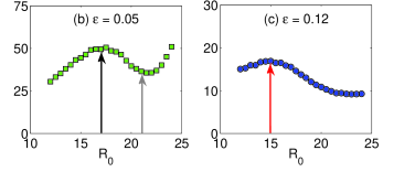
Figure 1: AET (measured in years) from simulations for the 1-city SIR model with $N=4\times 10^{5}$ (results for other population sizes are given in the SM, Figure S1). The arrows highlight the parameter regions where the attractor of the forced system changes from annual to biennial (black and red arrows), and from biennial to annual (grey arrow).

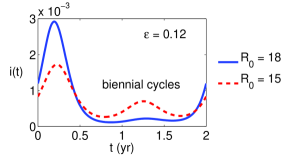
Figure 2: Fraction of infected as a function of time on the deterministic biennial attractor for the 1-city SIR model.

To illustrate the nontrivial interplay between disease transmissibility and amplitude of seasonal forcing we start in this section by studying the stochastic SIR model in a single city. The results are shown in Figure 1. For $\epsilon=0$, the AET increases exponentially with $R_{0}$, but a more complex dependence on $R_{0}$ is found when $\epsilon>0$. More specifically, for $\epsilon=0.05$ the AET gets larger as we increase $R_{0}$ from 12 to 17 where it attains a maximum. A further increase of $R_{0}$ reduces the AET, which reaches a minimum at $R_{0}\approx 21$ and starts to increase again from then on. For stronger seasonality, $\epsilon=0.12$, the curve describing the dependence of the AET on $R_{0}$ has only one maximum at about $R_{0}=15$. A similar effect was found in [5] for the dependence of persistence on birth rate. The dependence of the AET on $R_{0}$ is even more pronounced for larger population sizes, while it becomes less significant for smaller population sizes where frequent extinctions dominate all regimes (see Section 4 of Supplementary Material).

As in [24], a simple qualitative explanation of the behavior seen in Figure 1 can be given in terms of attractors of the deterministic model and their stability properties. For the unforced case, the attractor is a stable fixed point with nonzero densities of susceptible and infective individuals. As $R_{0}$ increases, the infective density associated with this attractor increases, as well as its stability. As a consequence, in the stochastic model the relative amplitude of the oscillations of the number of infected around their average value gets smaller, causing the AET to increase with $R_{0}$. In the presence of seasonality, $\epsilon>0$, the attractors of the system are limit cycles with periods multiples of 1 year. Depending on the values of $R_{0}$, only annual or biennial cycles are observed in the parameter ranges we explored. Specifically, for $\epsilon=0.12$ and $R_{0}\in[12,14.5]$ or $R_{0}\in[15,24]$, the cycles are annual or biennial, respectively. The period doubling bifurcation occurs in the interval $14.5\leq R_{0}\leq 15$ that separates the regions of increasing and decreasing extinction times. As shown in Figure 2, the deterministic biennial cycle changes with increasing $R_{0}$ so that the infective density stays low for a longer fraction of the period. Due to this, in the biennial regime the AET decreases with $R_{0}$. In the annual regime, the stability of the cycle and the infective density averaged over the cycle increase with $R_{0}$, explaining the increasing AET for $R_{0}\in[12,14.5]$ as in the unforced case. A similar analysis holds for $\epsilon=0.05$.

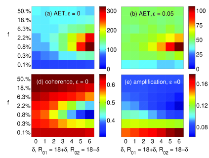
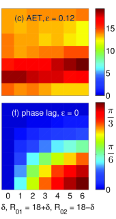
Figure 3: Results for the 2-city SIR model with $N_{1}=N_{2}=2\times 10^{5}$. In all panels, the x-axis represents the heterogeneity in terms of $\delta=(R_{01}-R_{02})/2$ and the why axis the coupling in terms of $f$. (a)-(c) AET (measured in years) as a function of the heterogeneity parameter $\delta$ and the coupling coefficient $f$ obtained from simulations for different levels of seasonality $\epsilon$ (notice the logarithmic scale in the $f$ axis). (d)-(f) Analytical results for the amplification and coherence in one of the cities (similar results for the other city are shown in the SM, Figure S2) and phase lag between cities for $\epsilon=0$.

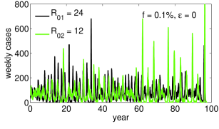
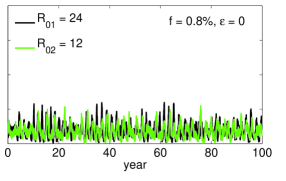
Figure 4: Typical time series of new disease cases per week for the 2-city SIR model with $N_{1}=N_{2}=2\times 10^{5}$ and $\epsilon=0$.

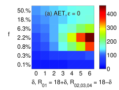
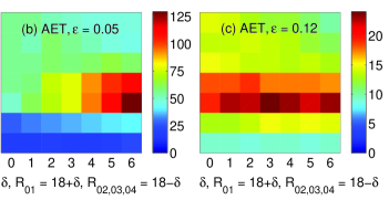
Figure 5: AET (measured in years) from simulations for the 4-city SIR model in which a central city with $N_{1}=2.1\times 10^{5}$ is surrounded by 3 non-interacting satellite cities with $N_{2}=N_{3}=N_{4}=N_{1}/3$. Fraction of commuters from each of the suburban cities to the central city, $f$, is 10 times larger than that from the central city to that suburban city. In all panels, the x-axis represents the heterogeneity in terms of $\delta=(R_{01}-R_{02})/2$. Analytical results for the amplification, coherence and phase lag of the fluctuations are given in the SM, Figure S3.

We now explore the situation where different population patches represent very different urban environments, as may be the case of an active city centre and its suburban satellite towns. We will therefore consider our model for two cities with different values of $R_{0}$, taking for simplicity equal population sizes and the symmetric coupling described in Section 2.1. The two values $R_{01}$ and $R_{02}$ that characterize SIR dynamics in each patch are given in terms of a single parameter $\delta$ as $18\pm\delta$, thus ensuring that the average disease infectiousness is kept constant as the spatial heterogeneity increases with $\delta$. The qualitative results are independent of this assumption (results not shown), which however reduces the number of free parameters and is consistent with the fact that estimates of $R_{0}$ come from coarse grained data. We will study the three levels of seasonality $\epsilon=0$, $0.05$, $0.12$ considered in the study of one city, and the free parameters for each value of $\epsilon$ are $\delta$ and the coupling strength $f$, the latter ranging from $f=0$ to the maximum meaningful value of $f=1/2$.

The results found for the AET (measured in years) are shown in Figure 3, top row. For the highest level of forcing, $\epsilon=0.12$, AETs are very short and the dependence on $f$ and $\delta$ is weak, with only a slight increase in persistence for small coupling strengths, independently of heterogeneity. This is in line with results reported in the literature for uniform systems [14], and can be understood as temporal heterogeneity superseding spatial heterogeneity for this level of seasonality, bringing the system close to extinction for a large part of the year.

The picture that emerges for $\epsilon=0$ and $\epsilon=0.05$ is significantly different. Extinction events are rare, and when spatial heterogeneity, measured by $\delta$, is small, the AET increases with the coupling strength $f$. This is to be expected, because disease that goes extinct in one of the identical patches is more likely to be reignited by surviving infectives in the other patch as $f$ increases. More surprisingly, a second and dominant effect of persistence enhancement shows up for intermediate coupling strengths when the degree of spatial heterogeneity is high.

In order to understand the causes of this remarkable increase in persistence, we have analyzed the amplification, the coherence and the phase difference for $\epsilon=0$ and all the parameter values used to compute the AETs. We have used the analytic approximations derived in the SM, which for the population sizes under consideration provide very good quantitative agreement with simulations. The results are shown in Figure 3, bottom row. In the left and middle panels, it can be seen that the enhanced persistence effect is associated with a reduction of the overall power of the infective number fluctuations and, more evidently, with a pronounced reduction of their coherence. In the right panel, we see that the phase lag between patches introduced by spatial heterogeneity, which would seem a good candidate to explain the observed effect, has no significant bearing on persistence.

In Figure 4 we plot two typical time series taken for $\delta=6$ and values of $f$ that correspond to extreme values of amplification and coherence in Figure 3. These plots illustrate how the amplification and coherence measures translate into the amplitude and structure of the fluctuations of the infective time series, and therefore into persistence as well. It can be seen that in the right panel the overall amplification is more evenly distributed over frequencies, so that large amplitude fluctuations are absent and local persistence is increased. Using the theory developed in [28], we show in the SM how this effect is associated with the dependence on $f$ and $\delta$ of the real part of one of the eigenvalue pairs of the linear approximation of the deterministic system at the endemic equilibrium.

Finally, in Figure 5 we show a plot of AETs similar to that of Figure 3, but in this case for a configuration of four population patches, one central city connected to three non-interacting satellite suburban areas with equal population sizes. The results shown correspond to the central city and to one of the suburban areas for the case when the fraction of commuters from each of the suburban cities to the central city, $f$, is 10 times larger than that from the central city to that suburban city. Both the phenomenological description and the theoretical interpretation given above for two cities hold in this case as well. The overall larger AETs in this case are due to the assymetric coupling, which increases the effective population size of the central city.

4 Discussion

Using a stochastic SIR metapopulation model with one population patch connected to one or several non-interacting patches, we have explored the combined effects on disease persistence of seasonality and spatial heterogeneity. The parameters in this analysis are the level of seasonality, the strength of the coupling, and the degree of heterogeneity measured by the difference between patches in the rates of potentially infectious contacts. We have considered only the simplest metapopulation structures and couplings. Results in more general settings (not shown) indicate that the effects described in this paper are robust with respect to different choices of these interaction parameters, and also to changes in the average $R_{0}$. In order to understand the mechanisms at play, we have compared for a large set of parameter choices the AETs found in the simulations with three main properties of the infective fluctuations: the amplitude, that measures the overall power, the coherence, that measures their regularity, and the phase lag between cities. These were computed for the unforced system using an analytic approximation developed in [28].

In contrast with spatially structured systems formed by similar patches [23], the inherent heterogeneity of the model has been shown to induce well defined phase lags in the epidemic bursts that take place in different patches [28], suggesting a simple mechanism through which heterogeneity might contribute to an increase in disease persistence. Indeed, in-phase abundance oscillations in different patches are often associated with global extinction [10, 3, 8].

However, we have found no clear evidence of such relation. This negative result can be understood because epidemic bursts come in short spikes, after which the system remains for a relatively long time close to extinction. The overall duration of the regime characterized by very low population numbers in two interacting patches is only slightly reduced by the phase lag. We speculate that in systems where the population fluctuations are smoother a relation between persistence and the phase lags due to spatial heterogeneity would be apparent.

We find instead a remarkable effect of enhanced persistence associated with strong spatial heterogeneity, intermediate coupling strength and moderate seasonal forcing. We should point out that the figures illustrating this effect are shown in logarithmic scale for the coupling strength $f$, and that therefore the range of values of $f$ that produce enhanced persistence is quite small. For these values however the extinction times raise very significantly, both for the unforced and the seasonally forced system, provided the forcing amplitude is not too large.

Enhanced persistence for intermediate coupling strengths has been reported for uniform metapopulation models [18, 15]. In these systems, the parameter values are the same in different patches, and spatial heterogeneity, instead of being built in the model, shows up only when the coupling strength is small enough for the dynamics in different patches to be practically uncorrelated. The increase of persistence at intermediate coupling expresses the trade-off between heterogeneity due to patch structure, which is lost at high coupling, and rescue events, which become negligible at low coupling.

One may try to carry this simple explanation over to the two patch model considered here. When the parameter values are similar in the two patches, the AET increases with the coupling strength and there is no phase lag between patches, suggesting that rescue effects are dominant in this regime. For highly heterogeneous patches, a phase lag shows up that decreases with coupling strength, while the number of rescue events increases, and the balance of these effects would explain the increase of persistence at intermediate coupling.

In this interpretation, the increase in persistence is a consequence of the patch structure, and not of a change in the properties of the fluctuations in each patch. However, comparison of the AETs with the properties of the fluctuation spectrum shows that, for the unforced system, enhanced global persistence is associated with a decrease in the coherence of the fluctuations in both patches and therefore with enhanced local persistence. As detailed in the SM, the analytic approximation can be used to show that this effect is related with an increase in the stability of the attractor that describes the system for very large population sizes. This analysis was carried out for the unforced case only, but we found the effect of enhanced persistence to be relatively insensitive to seasonal forcing, provided the forcing amplitude is not so strong that it drives the system close to extinction for a large period of the year [8]. We conclude that the effect of enhanced persistence documented here has to be traced back to the dependence of the stability of the attractor of the system on the coupling strength. Rather than being the result of rescue effects between population patches, it reflects an increase in local persistence induced by the coupling.

Financial support from the Portuguese Foundation for Science and Technology (FCT) under Contracts POCTI/ISFL/2/261 and (G.R.) SFRH/BPD/69137/2010 is gratefully acknowledged.

References

- [1] D. Balcan, V. Colizza, B. Goncalves, H. Hu, J. J. Ramasco, and A. Vespignani. Multiscale mobility networks and the spatial spreading of infectious diseases. Proc. Natl. Acad. Sci. USA, 106:21484–21489, 2009.
- [2] M. S. Bartlett. Measles periodicity and community size. J. R. Stat. Soc. A, 120:48–70, 1957.
- [3] B. Blasius, A. Huppert, and L. Stone. Complex dynamics and phase synchronization in spatially extended ecological systems. Nature, 399:354–359, 1999.
- [4] B. Bolker and B. T. Grenfell. Space, persistence and dynamics of measles epidemics. Phil. Trans. R. Soc. B, 348:309–320, 1995.
- [5] A. J. K. Conlan and B. T. Grenfell. Seasonality and the persistence and invasion of measles. Proc. R. Soc. B, 274:1133–1141, 2007.
- [6] D. J. D. Earn, P. Rohani, and B. T. Grenfell. Persistence, chaos and synchrony in ecology and epidemiology. Proc. R. Soc. B, 265:7–10, 1998.
- [7] D. Gillespie. A general method for numerically simulating the stochastic time evolution of coupled chemical reactions. J. Comp. Phys., 22:403–434, 1976.
- [8] N. C. Grassly and C. Fraser. Seasonal infectious disease epidemiology. Proc. R. Soc. B, 273:2541–2550, 2006.
- [9] B. T. Grenfell, O. N. Bjørnstad, and J. Kappey. Travelling waves and spatial hierarchies in measles epidemics. Nature, 414:716–723, 2001.
- [10] B. T. Grenfell, B. M. Bolker, and A. Kleczkowski. Seasonality and extinction in chaotic metapopulations. Proc. R. Soc. B, 259:97–103, 1995.
- [11] B. T. Grenfell and J. Harwood. (Meta)population dynamics of infectious diseases. TREE, 12:395–399, 1997.
- [12] T. J. Hagenaars, C. A. Donnelly, and N. M. Ferguson. Spatial heterogeneity and the persistence of infectious diseases. J. Theor. Biol., 229:349–359, 2004.
- [13] I. Hanski. Metapopulation dynamics. Nature, 396:41–49, 1998.
- [14] I. Hanski. Metapopulation Ecology. Oxford University Press, Oxford, 1999.
- [15] M. Jesse and H. Heesterbeek. Divide and conquer? Persistence of infectious agents in spatial metapopulations of hosts. J. Theor. Biol., 275:12–20, 2011.
- [16] A. Källén, P. Arcuri, and J. D. Murray J. A simple model for the spatial spread and control of rabies. J. Theor. Biol., 116:377–393, 1985.
- [17] M. J. Keeling, L. Danon, M. C. Vernon, and T. A. House. Individual identity and movement networks for disease metapopulations. Proc. Natl. Acad. Sci. USA, 107:8866–8870, 2010.
- [18] M. J. Keeling Metapopulation moments: Coupling, stochasticity and persistence. J. Anim. Ecol., 69:725–736, 2000.
- [19] M. J. Keeling and B. T. Grenfell. Understanding the persistence of measles: reconciling theory, simulation and observation. Proc. R. Soc. B, 269:335–343, 2002.
- [20] M. J. Keeling and P. Rohani. Estimating spatial coupling in epidemiological systems: a mechanistic approach. Ecol. Lett., 5:20–29, 2002.
- [21] R. Lande. Demographic stochasticity and Allee effect on a scale with isotropic noise. Oikos, 83:353–358, 1998.
- [22] R. Levins. Some demographic and genetic consequences of environmental heterogeneity for biological control. Bull. Entom. Soc. Am., 15:237–240, 1969.
- [23] A. L. Lloyd and R. M. May. Spatial heterogeneity in epidemic models. J. Theor. Biol., 179:1–11, 1996.
- [24] N. B. Mantilla-Beniers, O. N. Bjørnstad, B. T. Grenfell, and P. Rohani. Decreasing stochasticity through enhanced seasonality in measles epidemics. J. R. Soc. Interface, 7:727–739, 2010.
- [25] I. Nåsell. A new look at the critical community size for childhood infections. Theor. Pop. Biol., 67:203–216, 2004.
- [26] S. Riley. Large-scale spatial-transmission models of infectious disease. Science, 316:1298–1301, 2007.
- [27] G. Rozhnova, A. Nunes, and A. J. McKane. Stochastic oscillations in models of epidemics on a network of cities. Phys. Rev. E, 84:051919, 2011.
- [28] G. Rozhnova, A. Nunes, and A. J. McKane. Phase lag in epidemics on a network of cities. Phys. Rev. E, 85:051912, 2012.
- [29] H. E. Soper. The interpretation of periodicity in disease prevalence. J. R. Stat. Soc. A, 92:34–61, 1929.
- [30] L. Stone, R. Olinky, and A. Huppert. Seasonal dynamics of recurrent epidemics. Nature, 446:533–536, 2007.
- [31] N. G. van Kampen. Stochastic Processes in Physics and Chemistry. Elsevier, Amsterdam, 1981.
- [32] C. Viboud, O. N. Bjørnstad, D. L. Smith, L. Simonsen, M. A. Miller, and B. T. Grenfell. Synchrony, waves, and spatial hierarchies in the spread of influenza. Science, 312:447–451, 2006.
- [33] J. A. Yorke, N. Nathanson, G. Pianigiani, and J. Martin. Seasonality and the requirements for perpetuation and eradication of viruses in populations. Am. J. Epidemiol., 109:103–123, 1979.