A Polyhedral Approximation Framework for
Convex and Robust Distributed Optimization

Abstract

In this paper we consider a general problem set-up for a wide class of convex and robust distributed optimization problems in peer-to-peer networks. In this set-up convex constraint sets are distributed to the network processors who have to compute the optimizer of a linear cost function subject to the constraints. We propose a novel fully distributed algorithm, named cutting-plane consensus, to solve the problem, based on an outer polyhedral approximation of the constraint sets. Processors running the algorithm compute and exchange linear approximations of their locally feasible sets. Independently of the number of processors in the network, each processor stores only a small number of linear constraints, making the algorithm scalable to large networks. The cutting-plane consensus algorithm is presented and analyzed for the general framework. Specifically, we prove that all processors running the algorithm agree on an optimizer of the global problem, and that the algorithm is tolerant to node and link failures as long as network connectivity is preserved. Then, the cutting plane consensus algorithm is specified to three different classes of distributed optimization problems, namely (i) inequality constrained problems, (ii) robust optimization problems, and (iii) almost separable optimization problems with separable objective functions and coupling constraints. For each one of these problem classes we solve a concrete problem that can be expressed in that framework and present computational results. That is, we show how to solve: position estimation in wireless sensor networks, a distributed robust linear program and, a distributed microgrid control problem.

I Introduction

The ability to solve optimization problems by local data exchange between identical processors with small computation and communication capabilities is a fundamental prerequisite for numerous decision and control systems. Algorithms for such distributed systems have to work within the following specifications [1]. All processors running the algorithm are exactly identical and each processor has only a small memory available. The data assigned by the algorithm to a processor should be independent of the overall network size or only slowly growing with the degree of the processor node in the network. None of the processors has global information or can solve the problem independently.

This paper addresses a class of optimization problems in distributed processor networks with asynchronous communication. Distributed, or peer-to-peer, optimization is related to parallel [2] or large-scale optimization [3], but has to meet further requirements, such as asynchronous communication and lack of shared memory or coordination units. Distributed optimization has gained significant attention in the last years. Initially major attention was given to asynchronous distributed subgradient methods [4], [5]. Asynchronous distributed primal and dual subgradient algorithms are important tools in network utility maximization and have been intensively studied from a communication networks perspective, see [6], [7].

Combined with projection operations, subgradient methods can also solve constrained optimization problems [8], [6]. In the last years, the research scope has been widened and now several different distributed algorithms are explored, each suited for particular optimization problems. Distributed Newton methods are proposed for Network Utility Maximization [9], [10], or unconstrained strongly convex problems [11]. Distributed variants of Alternating Direction Method of Multipliers (ADMM) have been proposed for distributed estimation [12], and in the wider context of machine learning [13]. The ADMM shows often a good convergence rate. However, one structural difference between ADMM and distributed algorithms such as subgradient methods or the novel method proposed in this paper has to be emphasized. In a centralized implementation ADMM requires a coordination step. Distributed ADMM replaces this central coordination with a consensus algorithm. However, this requires a synchronization between all processors in the network, i.e., all processors have to switch synchronously between local computations and the consensus algorithm. Fully distributed algorithms, as the one proposed here, work asynchronously and every processor can switch between local computations and communications at its own pace.

An alternative research direction was established in [14] and [15], where distributed abstract optimization problems were considered. A similar approach was explored in [16], [17] for a distributed simplex algorithm that solves degenerate linear programs and multi-agent assignment problems. Some results on the use of distributed cutting-plane methods for robust optimization have been presented in [18]. The results of [18] are presented in the present paper in the wider context of general distributed optimization using cutting-plane methods.

The contributions of this paper are as follows. Motivated by several important applications, we consider a general distributed optimization framework in which each processor has knowledge of a convex constraint set and a linear cost function has to be optimized over the intersection of these constraint sets. It is worth noting that linearity of the cost function is not a limitation and that strict convexity of the optimization problem is not required. A novel fully distributed algorithm named cutting plane consensus is proposed to solve this class of distributed problems. The algorithm uses a polyhedral outer-approximation of the constraint set. Processors performing the algorithm generate and exchange a small and fixed number of linear constraints, which provide a polyhedral approximation of the original optimization problem. Then, each processor updates its local estimate of the globally optimal solution as the minimal 2-norm solution of the approximate optimization problem. We prove the correctness of the algorithm in the sense that all processor asymptotically agree on a globally optimal solution. We show that the proposed algorithm satisfies all requirements of peer-to-peer processor networks. In particular, it requires only a strictly bounded local memory and the communication is allowed to be asynchronous. We also prove that the algorithm has an inherent tolerance against the failure of single processors.

To highlight the generality of the proposed polyhedral approximation method, we show how it can solve three different representations of the general distributed convex program. First, we consider constraint sets defined by nominal convex inequality constraints. Second, we discuss the method for a class of uncertain or semi-infinite constraints. We show that the novel algorithm is capable of computing robust solutions to uncertain problems in peer-to-peer networks. Finally, we show that almost separable convex programs, i.e., convex optimization problems with separable objective functions and coupling constraints, can be formulated in the general framework when their dual representation is considered. Applied to this problem class the Cutting-Plane Consensus algorithm can be seen as a fully distributed version of the classical Dantzig-Wolfe decomposition, or column generation method, with no central coordinating master program.

The general algorithm derived in the paper applies directly to each of the three problem classes, and all convergence guarantees remain valid. We present for each problem class a relevant decision problem, which can be solved by the novel algorithm. In particular, it is shown that localization in sensor networks, robust linear programming and distributed control of microgrids can be solved by the algorithm. Additionally, computational studies are presented which show that the novel algorithm has an advantageous time complexity.

Relation to other optimization methods: The general problem formulation of this paper is similar to the formulation considered in [8]. However, while the approach in [8] requires a projection operation, which might be computationally expensive for some constraint classes, our approach requires only the knowledge of a polyhedral approximation. Additionally, our method works on general time-varying directed graphs, and does not require a balanced communication.

The almost separable optimization problem setup studied in Section VII is the classical setup for large scale optimization. Dual decomposition methods decompose these problems into a master program and several subproblems. Cutting-plane methods can be used to solve the master program, leading to algorithms that originate in the classical Dantzig-Wolfe decomposition [19], [3]. The algorithm we propose differs significantly from classical decomposition methods. Indeed, our algorithm performs in asynchronous peer-to-peer networks with identical processors, without any central or coordinating master program.

A distributed ADMM implementation [13] uses an average consensus algorithm to replace the update of the central master program. While this allows to perform all computations decentralized, it requires a synchronization between the processors. Additionally, preforming a consensus algorithm repeatedly might require many communication steps between the processors. In contrast, our method requires neither synchronized communication nor a repeated averaging.

The remainder of the paper is organized as follows. The optimization problem and the processor network model are introduced in Section II. In Section III the ideas of polyhedral outer-approximation and minimal norm linear programming are reviewed. The main contribution of this paper, the Cutting-Plane Consensus algorithm, is presented in a general form in Section IV, where also the correctness of the algorithm and its fault-tolerance are proven. The application of the algorithm to inequality constrained problems and to a localization problem in sensor networks is presented in Section V. In Section VI it is shown how the algorithm can be used to solve distributed robust optimization problems, and a computational study is presented, which compares the completion time of the novel algorithm to an ADMM algorithm. The application of the Cutting-Plane Consensus algorithm to almost separable convex optimization problems and to distributed microgrid control is discussed in Section VII. Finally, a concluding discussion is given in Section VIII.

II Problem Formulation and Network Model

We consider a set of processors $V=\{1,\ldots,n\}$, each equipped with communication and computation capabilities. Each processor $i$ has knowledge of a convex and closed constraint set $\mathcal{Z}_{i}\subset\mathbb{R}^{d}$. The processors have to agree on a decision vector $z\in\mathbb{R}^{d}$ maximizing a linear objective over the intersection of all sets $\mathcal{Z}_{i}$. That is, the processors have to solve the distributed convex optimization problem

$$\begin{split}\text{maximize}&\quad c^{T}z\\ \text{subject to}&\quad z\in\bigcap_{i=1}^{n}\mathcal{Z}_{i}.\end{split}$$ (1)

We denote the feasible set in the following as $\mathcal{Z}:=\bigcap_{i=1}^{n}\mathcal{Z}_{i}$. We assume that $\mathcal{Z}$ is non-empty and that (1) has a finite optimal solution.

The communication between the processors is modeled by a directed graph (digraph) $\mathcal{G}_{c}=(V,E)$, named communication graph. The node set $V=\{1,\ldots,n\}$ is the set of processor identifiers, and the edge set $E\subset\{1,\ldots,n\}^{2}$ characterizes the communication among the processors. If the edge-set does not change over time, the graph is called static otherwise it is called time-varying. We model the communication with time-varying digraphs of the form $\mathcal{G}_{c}(t)=(V,E(t))$, where $t\in\mathbb{N}$ represents a slotted universal time. A graph $\mathcal{G}_{c}(t)$ models the communication in the sense that at time $t$ there is an edge from node $i$ to node $j$ if and only if processor $i$ transmits information to processor $j$ at time $t$. The time-varying set of outgoing (incoming) neighbors of node $i$ at time $t$, i.e., the set of nodes to (from) which there are edges from (to) $i$ at time $t$, is denoted by $\mathcal{N}_{O}(i,t)$ ($\mathcal{N}_{I}(i,t)$). In a static directed graph, the minimum number of edges between node $i$ and $j$ is called the distance from $i$ to $j$ and is denoted by $\operatorname{dist}(i,j)$. The maximum $\operatorname{dist}(i,j)$ taken over all pairs $(i,j)$ is the diameter of the graph $\mathcal{G}_{c}$ and is denoted by $\operatorname{diam}(\mathcal{G}_{c})$. A static digraph is said to be strongly connected if for every pair of nodes $(i,j)$ there exists a path of directed edges that goes from $i$ to $j$. For the time-varying communication graph we rely on the concept of a jointly strongly connected graph.

Assumption II.1 (Joint Strong Connectivity)

For every time instant $t\in\mathbb{N}$, the union digraph $\mathcal{G}_{c}^{\infty}(t):=\cup_{\tau=t}^{\infty}\mathcal{G}_{c}(\tau)$ is strongly connected. $\square$

In this paper we develop a distributed, asynchronous algorithm solving problem (1) according to the network model described above. Each processor stores a small set of data and transmits at each time instant these data to its out-neighbors $\mathcal{N}_{O}(i,t)$. It is worth noting that in general it is impossible to encode the convex set $\mathcal{Z}_{i}$ with finite data. Thus, the information about the sets $\mathcal{Z}_{i}$ cannot be explicitly exchanged among the processors.

III Polyhedral Approximation and Minimal Norm Linear Programming

We start recalling some important concepts form convex and linear optimization. We will work in the following with half-spaces of the form $\mathit{h}:=\{z:a^{T}z-b\leq 0\},$ where $a\in\mathbb{R}^{d}$ and $b\in\mathbb{R}$. A half-space is called a cutting-plane if it satisfies the following properties. Given a closed convex set $\mathcal{S}\subset\mathbb{R}^{d}$ and a query point $z_{q}\notin\mathcal{S}$, a cutting-plane $h(z_{q})$ separates $z_{q}$ from $\mathcal{S}$, i.e., $a(z_{q})\neq 0$ and

$$a^{T}(z_{q})z\leq b(z_{q})\quad\mbox{for\;all}\;z\in\mathcal{S},\quad\mbox{and}\quad a^{T}(z_{q})z_{q}-b(z_{q})=s(z_{q})>0.$$ (2)

The concept of cutting-planes leads to the first algorithmic primitive, the cutting-plane oracle.

Cutting-Plane Oracle $\operatorname{ORC}(z_{q},\mathcal{S})$: queried at $z_{q}\in\mathbb{R}^{d}$ for the set $\mathcal{S}$. If (i) $z_{q}\notin\mathcal{S}$ then it returns a cutting-plane $\mathit{h}(z_{q})$, separating $z_{q}$ and $\mathcal{S}$, otherwise (ii) it asserts that $z_{q}\in\mathcal{S}$ and returns an empty $\mathit{h}$.

We make the following assumption on the cutting plane oracle, following the general cutting-plane framework of [20].

Assumption III.1

The cutting-plane oracle $\operatorname{ORC}(z_{q},\mathcal{S})$ is such that (i) $\|a(z_{q})\|_{2}<\infty$ and (ii) $z_{q}(t)\rightarrow\bar{z}$ and $s(z_{q}(t))\rightarrow 0$ implies that $\bar{z}\in\mathcal{S}.$

Note that this assumption is not very restrictive and holds for many important problem formulations. In fact, we discuss three important problem classes for which the assumption holds.

Given a collection of cutting-planes $H=\cup_{k=1}^{m}\mathit{h}_{k}$, the polyhedron induced by these cutting-planes is $\mathcal{H}=\{z:A_{H}^{T}z\leq b_{H}\}$, with the matrix $A_{H}\in\mathbb{R}^{d\times m}$ as $A_{H}=[a_{1},\ldots,a_{m}]$, and the vector $b_{H}=[b_{1},\ldots,b_{m}]^{T}$.

Remark III.2 (Cutting plane notation)

We refer to both a half-space $h$ and the data inducing the half space with a small italic letter. A collection of cutting-planes is denoted with italic capital letters, e.g., $H=\bigcup_{k=1}^{m}h_{k}$. For a collection of cutting-planes, we denote the induced polyhedron with capital calligraphic letters, e.g., $\mathcal{H}$. Please note the following notational aspect. A collection of cutting-planes $B$ that is a subset of the cutting-planes contained in $H$ is denoted as $B\subset H$, while the induced polyhedra satisfy $\mathcal{B}\supseteq\mathcal{H}$. $\square$

Assume that each cutting-plane $h_{i}$ is generated as a separating hyperplane for some set $\mathcal{Z}_{j}$, and let $H$ be a collection of cutting-planes. The linear approximate program

$$\begin{split}\max_{z}&\quad c^{T}z\quad\mathrm{s.t.}\;A_{H}^{T}z\leq b_{H}\end{split}$$ (3)

is then a relaxation of the original optimization problem (1) since the polyhedron $\mathcal{H}=\{z:A_{H}^{T}z\leq b_{H}\}$ is an outer approximation of the original constraint set $\mathcal{Z}=\bigcap_{i=1}^{n}\mathcal{Z}_{i}$. We denote in the following the optimal value of (3) as $\gamma_{H}$, i.e., $\gamma_{H}:=\max_{z\in\mathcal{H}}c^{T}z$. The linear program (3) has in general several optimizers, and we denote the set of all optimizers of (3) with

$$\Gamma_{H}:=\{z\in\mathcal{H}:\;c^{T}z\geq c^{T}v,\forall v\in\mathcal{H}\}.$$ (4)

It is a standard result in linear programming that $\Gamma_{H}$ is always a polyhedral set. We consider throughout the paper the unique optimal solution to (3) which has the minimal 2-norm, i.e., we aim to compute

$$z_{H}^{*}=\mathrm{arg}\min_{z\in\Gamma_{H}}\|z\|_{2}.$$ (5)

Finding a minimal norm solution to a linear program is a classical problem and various solution methods are proposed in the literature. Starting from the early reference [21] research on this topic is still actively pursued [22]. The minimal 2-norm solution can be efficiently computed as the solution of a quadratic program.

Proposition III.3

Let $u^{*}\in\mathbb{R}^{|H|},\alpha^{*}\in\mathbb{R},l^{*}\in\mathbb{R}^{d}$ be the optimal solution to

$$\begin{split}\min_{u,\alpha,l}\quad&\frac{1}{2}(A_{H}u+\alpha c)^{T}(A_{H}u+\alpha c)+b_{H}^{T}u+c^{T}l\\ \mathrm{s.t.}\quad&A_{H}^{T}l-\alpha b\geq 0,\;u\geq 0\end{split}$$ (6)

then $z^{*}_{H}=-A_{H}u^{*}-\alpha^{*}c$ solves (5). $\square$

The proof of this result is presented in Appendix A. The minimal 2-norm solution has the important property that it always maximizes a strongly concave cost function.

Lemma III.4

Let a set of cutting-planes define the polyhedron $\mathcal{H}$ and let $z^{*}_{H}$ be the minimal 2-norm solution to (3). Consider the quadratically perturbed linear objective

$$J_{\epsilon}(z)=c^{T}z-\frac{\epsilon}{2}\|z\|^{2}_{2}$$

parametrized with a constant $\epsilon>0$. Then there exists a $\bar{\epsilon}>0$ such that for any $\epsilon\in[0,\bar{\epsilon}]$

$$z^{*}_{H}=\mathrm{arg}\max_{z\in\mathcal{H}}\;J_{\epsilon}(z).$$ (7)

$\square$

The proof of this result is very similar to the classical proof presented in [23]. However, since the considered set-up is slightly different and the result is fundamental for the methodologies developed in the paper, we present the proof in Appendix B.

Any solution to a (feasible) linear program of the form (3) is fully determined by at most $d$ constraints. This is naturally also true for the minimal 2-norm solution of a linear program. We formalize this property with the notion of basis. Given a collection of cutting-planes $H$, we say that a subset $B\subseteq H$ is a basis of $H$ if the minimal 2-norm solution to the linear program defined with the constraint set $B$, say $z_{B}^{*}$, is identical to the minimal 2-norm solution of the linear program defined with the constraint set $H$, say $z_{H}^{*}$, i.e., $z_{B}^{*}=z_{H}^{*}$, while for any strict subset of cutting-planes $B^{\prime}\subset B$, it holds that $z_{B^{\prime}}^{*}\neq z_{B}^{*}$. For a feasible problem, the cardinality of a basis is bounded by the dimension of the problem, i.e., $|B|\leq d$. Throughout this paper, a basis is always considered to be a basis with respect to the 2-norm solution of the linear program and a basis computation requires to compute the solution to problem (6). Note, however, that the active constraints at an optimal point $z_{H}^{*}$ are always a superset of a basis at this point and are exactly a basis if the problem is not degenerate. Therefore, in most cases it will be sufficient to find the active constraints, which are easy to detect.

IV The Cutting-Plane Consensus Algorithm

For a network of processors, we propose and analyze the Cutting-Plane Consensus algorithm to solve distributed convex optimization problems of the form (1).

The Distributed Cutting-Plane Consensus Algorithm

The algorithm to solve general distributed optimization problems (1) is as follows.

Cutting-Plane Consensus: Processors store and update collections of cutting-planes. The cutting-planes stored by agent $i$ at iteration $t$ are always a basis of a corresponding linear approximate program (3), and are denoted by $B^{[i]}(t)$. A processor initializes its local collection of cutting-planes $B^{[i]}_{0}$ with a set of cutting-planes chosen such that $\mathcal{B}^{[i]}_{0}\supset\mathcal{Z}_{i}$ and $\max_{z\in\mathcal{B}^{[i]}_{0}}c^{T}z<\infty$.

Each processor repeats then the following steps:

1. it transmits its current basis $B^{[i]}(t)$ to all its out-neighbors $\mathcal{N}_{O}(i,t)$ and receives the basis of its in-neighbors $Y^{[i]}(t)=\bigcup_{j\in\mathcal{N}_{I}(i,t)}B^{[j]}(t)$;

2. it defines $H_{tmp}^{[i]}(t)=B^{[i]}(t)\cup Y^{[i]}(t)$, and computes (i) a query point $z^{[i]}(t)$ as the minimal 2-norm solution to the approximate program (3), i.e.,

   $$z^{[i]}(t)=\mathrm{arg}\min_{z\in\Gamma_{H_{tmp}^{[i]}(t)}}\|z\|_{2}$$

   and (ii) a minimal set of active constraints $B_{tmp}^{[i]}(t)$;

3. it calls the cutting-plane oracle for the constraint set $\mathcal{Z}_{i}$ at the query point $z^{[i]}(t)$,

   $$h(z^{[i]}(t))=\operatorname{ORC}(z^{[i]}(t),\mathcal{Z}_{i});$$

4. it updates its collection of cutting planes as follows: if $z^{[i]}(t)\in\mathcal{Z}_{i}$ then $B^{[i]}(t+1)=B_{tmp}^{[i]}(t)$, otherwise $B^{[i]}(t+1)$ is set to the minimal basis of $B_{tmp}^{[i]}(t)\cup h(z^{[i]}(t))$.
   

The four steps of the algorithm can be summarized as communication (S1), computation of the query point (S2), generation of cutting-plane (S3) and dropping of all inactive constraints (S4). The Cutting-Plane Consensus algorithm is explicitly designed for the use in processor networks. We want to emphasize here the following four aspects of the algorithm.

Each processor can initialize the local constraint sets as a basis of the artificial constraint set $\{z\in\mathbb{R}^{d}:-M\boldsymbol{1}\leq z\leq M\boldsymbol{1}\}$ for some $M\gg 1$. If $M\in\mathbb{R}_{>0}$ is chosen sufficiently large, the artificial constraints will be dropped during the evolution of the algorithm.

Each processor stores and transmits at most $(d+1)d$ numbers at a time. In particular, processors exchange bases of (3), which are defined by not more than $d$ cutting-planes. Each cutting-plane is fully defined by $d+1$ numbers.

Each processor has to compute locally the 2-norm solution to a linear program with $d(|\mathcal{N}_{I}(i,t)|+1)$ constraints.

The Cutting-Plane Consensus algorithm does not require a time-synchronization. Each processor can perform its local computations at any speed and update its local state whenever it receives data from some of its in-neighbors.

Due to these properties, the Cutting-Plane Consensus algorithm is particularly well suited for optimization in large networks of identical processors.

Technical Analysis of the Cutting-Plane Consensus Algorithm

Before starting the proof of the algorithm correctness, we point out three important technical properties related to its evolution:

• The linear constraints stored by a processor form always a polyhedral outer-approximation of the globally feasible set $\mathcal{Z}$.

• The cost-function of each processor is monotonically non-increasing over the evolution of the algorithm.

• If the communication graph $\mathcal{G}_{c}$ is a strongly connected static graph, then after $\operatorname{diam}(\mathcal{G}_{c})$ communication rounds, all processors in the network compute a query-point with a cost not worse than the best processor at the initial iteration.

These properties provide an intuition about the functionality of the algorithm and the line we will follow to prove its correctness. They are formalized and proven rigorously in Lemma I.1 in Appendix I-B. We are ready to establish the correctness of the Cutting-Plane Consensus algorithm. We start by formalizing two auxiliary results which are also interesting on their own. The first result states the convergence of the query points to the locally feasible sets.

Lemma IV.1 (Convergence)

Assume Assumption III.1 holds. Let $z^{[i]}(t)$ be the query point generated by processor $i$ performing the Cutting-Plane Consensus algorithm. Then, the sequence $\{z^{[i]}(t)\}_{t\geq 0}$ has a limit point in the set $\mathcal{Z}_{i}$, i.e., there exists $\bar{z}^{[i]}\in\mathcal{Z}_{i}$ such that

$$\lim_{t\rightarrow\infty}\;\|z^{[i]}(t)-\bar{z}^{[i]}\|_{2}\rightarrow 0. \square$$

The second result shows that all processors in the network will reach an agreement.

Lemma IV.2 (Agreement)

Assume the communication network $\mathcal{G}_{c}(t)$ is jointly strongly connected. Let $z^{[i]}(t)$ be query points generated by the Cutting-Plane Consensus algorithm, then

$$\lim_{t\rightarrow\infty}\;\|z^{[i]}(t)-z^{[j]}(t)\|_{2}\rightarrow 0,\quad\mbox{for\; all\;}i,j\in\{1,\ldots,n\}. \square$$

The correctness of the algorithm is summarized in the following theorem.

Theorem IV.3 (Correctness)

Let $\mathcal{G}_{c}(t)$ be a jointly strongly connected communication network with processors performing the Cutting-Plane Consensus algorithm, and let Assumption III.1 hold. Let $z^{*}$ be the unique optimizer to (1) with minimal 2-norm, then

$$\lim_{t\rightarrow\infty}\|z^{[i]}(t)-z^{*}\|_{2}\rightarrow 0\quad\mbox{for\;all}\;i\in\{1,\ldots,n\}. \square$$

For the clarity of presentation, the technical proofs of Lemma IV.1, Lemma IV.2, and Theorem IV.3 are presented in Appendix I-B.

A major advantage for using the Cutting-Plane Consensus algorithm in distributed systems is its inherent fault-tolerance. The requirements on the communication network are very weak and the algorithm can well handle disturbances in the communication like, e.g., packet-losses or delays. Additionally, the algorithm has an inherent tolerance against processor failures. We say that a processor fails if it stops at some time $t_{f}$ to communicate with other processors.

Theorem IV.4 (Fault-Tolerance)

Suppose that processor $l$ fails at time $t_{f}$, and that the communication network remains jointly strongly connected after the failure of processor $l$. Let $z^{[l]}(t_{f})$ be the last query point computed by processor $l$ and define $\gamma^{[l]}(t_{f})=c^{T}z^{[l]}(t_{f})$. Then the query-points computed by all processors converge, i.e., $\lim_{t\rightarrow\infty}\|z^{[i]}(t)-\bar{z}_{-l}\|\rightarrow 0,$ with $\bar{z}_{-l}$ satisfying

$$\bar{z}_{-l}\in\left(\bigcap_{i\neq l}\mathcal{Z}_{i}\right)\quad\mbox{and}\quad c^{T}\bar{z}_{-l}\leq\gamma^{[l]}(t_{f}).$$

Proof:

Consider the evolution of the algorithm starting at time $t_{f}$. With Lemma IV.1 and Lemma IV.2 one can conclude that for all processors $i\neq l$, the query points will converge to the set $\left(\bigcap_{i\neq l}\mathcal{Z}_{i}\right)$. Additionally, the out-neighbors of the failing processor $l$ have received a basis $B^{[l]}(t_{f})$ such that the optimal value of the linear approximate program (3) is $\gamma^{[l]}(t_{f})$. Any query point $z^{[i]}(t),t\geq t_{f}$, subsequently computed by the out-neighbors of processor $l$ as the solution to (3) must therefore be such that $c^{T}z^{[i]}(t)\leq\gamma^{[l]}(t_{f})$ for all $t\geq t_{f}$. ∎

This last result provides directly a paradigm for the design of fault-tolerant systems.

Corollary IV.5

Suppose that for all $l\in V$, $\bigcap_{i=1,i\neq l}^{n}\mathcal{Z}_{i}=\mathcal{Z}$. Then for all $l\in V$, $\bar{z}_{-l}=z^{*}$ with $z^{*}$ the optimal solution to (1). $\square$

The abstract problem formulation (1) and the Cutting-Plane Consensus algorithm provide a general framework for distributed convex optimization. We show in the following that a variety of important representations of the constraint sets are covered by this set-up. Depending on the formulation of the local constraint sets $\mathcal{Z}_{i}$ different cutting-plane oracles must be defined, leading to different realizations of the algorithm. We specify in the following the Cutting-Plane Consensus algorithm to three important problem classes. We want to stress that the correctness proofs established here for the general set-up will hold directly for the three specific problem formulations discussed in the remainder of the paper.

V Convex Optimization with Distributed Inequality Constraints

As first concrete setup, we consider the most natural realization of the general problem formulation (1) with the local constraint set defined by a convex inequality, i.e.,

$$\mathcal{Z}_{i}=\{z:f_{i}(z)\leq 0\}.$$ (8)

The functions $f_{i}:\mathbb{R}^{d}\mapsto\mathbb{R}$ are assumed to be convex, but not necessarily differentiable. Thus, the set-up (8) includes also the case in which processor $i$ is assigned more that one constraint, say $\mathcal{Z}_{i}=\{z:f_{i1}(z)\leq 0,f_{i2}(z)\leq 0,\ldots,f_{ik}(z)\leq 0\}$. In fact, one can define $f_{i}(z):=\max_{j\in\{1,\ldots k\}}f_{ij}(z)$ and directly obtain the formulation (8).

To define a cutting-plane oracle for constraints of the form (8), we use the concept of subdifferential. Given a query-point $z_{q}\in\mathbb{R}^{d}$, the subdifferential of $f_{i}$ at $z_{q}$ is

$$\partial f_{i}(z_{q})=\{g_{i}\in\mathbb{R}^{d}:f_{i}(z)-f_{i}(z_{q})\geq g_{i}^{T}(z-z_{q}),\;\forall z\in\mathbb{R}^{d}\}.$$

An element $g_{i}\in\partial f_{i}(z_{q})$ is called a subgradient of $f_{i}$ at $z_{q}$. If the function $f_{i}$ is differentiable, then its gradient $\nabla f_{i}(z_{q})$ is a subgradient. A cutting-plane oracle for constraints of the form (8) is now as follows, see, e.g., [24].

Cutting-plane Oracle: If a query point $z_{q}$ is such that $f_{i}(z_{q})>0$, then

$$f_{i}(z_{q})+g_{i}^{T}(z-z_{q})\leq 0,$$ (9)

for some $g_{i}\in\partial f_{i}(z)$, is returned, .

Note also that Assumption III.1 is satisfied, since $s(z_{q})=f_{i}(z_{q})+g_{i}^{T}(z_{q}-z_{q})=f(z_{q})$, and $f(z_{q})=0$ implies $z_{q}\in\mathcal{Z}_{i}$. If $f_{i}(z):=\max_{j\in\{1,\ldots k\}}f_{ij}(z)$, then $\partial f_{i}(z_{q})=\mathbf{Co}\cup\{\partial f_{ij}(z_{q}):f_{ij}(z_{q})=f_{i}(z_{q})\}$, where $\mathbf{Co}$ denotes the convex hull. Thus, the method is applicable for constraints where subgradients can be obtained.

Remark V.1

An important class of constraints are semi-definite constraints of the form $\mathcal{Z}_{i}=\{z:F_{i}(z):=F_{i0}+z_{1}F_{i1}+\cdots+z_{d}F_{id}\leq 0\},$ where $F_{ij}$ are real symmetric matrices, and ${}^{\prime}\leq 0^{\prime}$ denotes negative semi-definite. The semi-definite constraint can be formulated as inequality constraint

$$f_{i}(z):=\lambda_{\max}(F_{i}(z))\leq 0,$$

with $\lambda_{\max}$ the largest eigenvalue of $F(z)$. It is discussed, e.g., in [25], that given a query point $z_{q}$ and a normalized eigenvector $v_{q}^{*}$ of $F_{i}(z_{q})$ corresponding to $\lambda_{\max}(F_{i}(z_{q}))$, then the vector $g_{i}=[v_{q}^{*T}F_{1}v_{q}^{*},\ldots,v_{q}^{*T}F_{d}v_{q}^{*}]^{T}$ is a subgradient of $f_{i}(z)$. The Cutting-Plane Consensus algorithm can thus handle semi-definite constraints and has to be seen in the context of the recent work on cutting-plane methods for semi-definite programming [26], [27]. $\square$

The Cutting-Plane Consensus algorithm is directly applicable to problems where processors are assigned convex, possibly non-differentiable, inequality constraints. Such distributed problems appear in various important application. For example, the distributed position estimation problem in wireless sensor networks can be formulated in the form (1) with convex inequality and semi-definite constraints available only locally to (some of) the sensor nodes.

Application Example: Convex Position Estimation in Wireless Sensor Networks

Wide-area networks of cheap sensors with wireless communication are envisioned to be key elements of modern infrastructure systems. In most applications, only few sensors are equipped with localization tools, and it is necessary to estimate the position of the other sensors, see [28].

In [29] the sensor localization problem is formulated as a convex optimization problem, which is then solved by a central unit using semidefinite programming. The semi-definite formulation proposed in [29] has been later extended in the literature. We formulate the distributed position estimation problem given in [29] in the general distributed convex optimization framework (1) and show that the general Cutting-Plane Consensus algorithm can be used for a fully distributed solution, using only local message passing between the sensors.

Let in the following $\mathbf{v}_{i}\in\mathbb{R}^{2}$ denote the known position of sensor $i\in\{1,\ldots,n\}$. We want to estimate the unknown position of an additional sensor $z\in\mathbb{R}^{2}$. In [29], two different estimation mechanisms are considered: (i) laser transmitters at nodes which scan through some angle, leading to a cone set, which can be expressed by three linear constraints of the form $f(z):=a_{i}^{T}z-b_{i}\leq 0,$ $a_{i}\in\mathbb{R}^{2\times 1}$ and $b_{i}\in\mathbb{R}$, two bounding the angle and one bounding the distance and (ii) the range of the RF transmitter, leading to circular constraints of the form $\|z-\mathbf{v}_{i}\|_{2}^{2}\leq r_{i}^{2}$. Using the Schur-complement, the quadratic constraint can be formulated as a semi-definite constraint of the form

$$F_{i}(z):=(-1)\begin{bmatrix}r_{i}I_{2}&(z-\mathbf{v}_{i})\\ (z-\mathbf{v}_{i})^{T}&r_{i}\end{bmatrix}\leq 0,$$

where $I_{2}$ is the $2\times 2$ identity matrix.

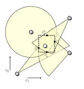
Figure 1: Localization of the white node by set estimates of the four gray nodes. The set estimate is given by the bounding box which determined by the four point $z_{x}^{l},z_{x}^{u},z_{y}^{l},z_{y}^{u}$. The four extreme points can be found with the Cutting-Plane Consensus algorithm.

Each sensor $i$ can bound the position of the unknown sensor to be contained in the convex set $\mathcal{Z}_{i}$, which is, depending on the available sensing mechanism, a disk represented by a semi-definite constraint $\mathcal{Z}_{i}=\{z:F_{i}(z)\leq 0\}$, a cone $\mathcal{Z}_{i}=\{z:f_{ij}(z)\leq 0,j=1,2,3\}$, or a quadrant, $\mathcal{Z}_{i}=\{z:F_{ij}(z)\leq 0,f_{ij}\leq 0,j=1,2,3\}$.

The sensing nodes can now compute the smallest box $\{z\in\mathbb{R}^{2}:[z^{l}_{x},z^{l}_{x}]^{T}\leq z\leq[z^{u}_{x},z^{u}_{y}]^{T}\}$ that is guaranteed to contain the unknown position using the Cutting-Plane Consensus algorithm. As proposed in [29], the minimal bounding box can be computed by solving four optimization problems with linear objectives. To compute, for example, $z^{u}_{x}$ one defines the objective $c_{x}=[1,0]^{T}$ and solves $z^{u}_{x}:=\max\;c_{x}^{T}z,\;\mbox{s.t.}\;z\in\bigcap_{i=1}^{n}\mathcal{Z}_{i}.$ In the same way $z^{l}_{x},z^{l}_{y},z^{u}_{y}$ can be determined. Figure 1 illustrates a configuration where four nodes estimate the position of one node. A linear version of such a distributed estimation problem, i.e., with all constraints being linear inequalities, has been considered in the previous work [15].

VI Robust Optimization with Uncertain Constraints

The general formulation (1) covers also distributed robust optimization problems with uncertain constraints. The Cutting-Plane Consensus algorithm can therefore be used to solve a class of robust optimization problems in peer-to-peer processor networks.

In particular, we consider constraint sets with parametric uncertainties of the form

$$\mathcal{Z}_{i}=\{z:\;f_{i}(z,\theta)\leq 0,\;\mbox{for\; all\;}\theta\in\Omega_{i}\}$$ (10)

where $\theta_{i}$ is an uncertain parameter, taking values in the compact convex set $\Omega_{i}$. We assume that $f_{i}$ is convex in $z$ for any fixed $\theta$. If additionally $f_{i}$ is concave in $\theta$ and $\Omega_{i}$ is a convex set, we say that the resulting optimization problem (1) is convex [30]. As we will see later on, the first condition is cruicial for the application of the algorithm. The second condition will ensure that the problem can be solved exactly by our algorithm.

The problem (1) with constraints of the form (10) is a distributed deterministic robust [31] or distributed semi-infinite optimization problem [30]. Each processor has knowledge of an infinite number of constraints, determined by the parameter $\theta$ and the uncertainty set $\Omega_{i}$. Obviously, uncertain constraints as (10) appear frequently in distributed decision problems. Here we focus on a deterministic worst-case optimization problem, where a solution that is feasible for any possible representation of the uncertainty is sought. A comprehensive theory for robust optimization in centralized systems has been developed and is presented, e.g., in [31].

Nowadays, mainly two different approaches are pursued in robust optimization. In one research direction infinite, uncertain constraints are replaced by a finite number of “sampled” constraints. Sampling methods select a finite number of parameter values and provide bounds for the expected violation of the uncertain constraints [32]. In a distributed setup, a sampling approach has been explored in [33]. The other research direction aims at formulating robust counterparts of the uncertain constraints (10), leading often to nominal semi-definite problems (see, e.g., [31]). Handling the uncertain constraint from a semi-infinite optimization point of view (10), allows also to apply exchange methods [34], where the sampling point is chosen as the solution of a finite approximation of the optimization problem. Recently, cutting-plane methods have been considered in the context of centralized robust optimization [35]. Robust optimization in processor networks is a relatively new problem. Robust optimization for communication networks using dual decomposition is considered in [36]. We connect the robust optimization problem with uncertain constraints (10) to our general distributed optimization framework, and show that the Cutting-Plane Consensus algorithm can solve the problem in processor networks. In fact, the novel Cutting-Plane Consensus algorithm is related to the exchange and cutting-plane methods [34], [35]. We define the cutting-plane oracle for the distributed robust optimization problem (10) as follows.

Pessimizing Cutting-Plane Oracle: Given a query point $z_{q}$, the worst-case parameter value $\theta_{q}^{*}$ is the maximizer of the optimization problem

$$\max_{\theta} \;f_{i}(z_{q},\theta)\;\quad\mathrm{s.t.}\;\theta\in\Omega_{i}.$$ (11)

The query point $z_{q}$ is contained in $\mathcal{Z}_{i}$ if and only if the value of (11) is smaller or equal to zero. If $z_{q}\notin\mathcal{Z}_{i}$, then cutting-plane is generated as

$$f_{i}(z_{q},\theta_{q}^{*})+g_{i}^{T}(z-z_{q})\leq 0$$ (12)

where $g_{i}^{T}\in\partial f_{i}(z_{q},\theta_{q}^{*})$ is a subgradient of $f_{i}$.

To see that (12) is a cutting-plane, note that a query point $z_{q}\notin\mathcal{Z}_{i}$ is cut off, since $f_{i}(z_{q},\theta_{q}^{*})+g_{i}^{T}(z_{q}-z_{q})=f_{i}(z_{q},\theta_{q}^{*})>0$. Additionally, for any point $z\in\mathcal{Z}_{i}$, we have $0\geq f_{i}(z_{i},\theta)$ for all $\theta\in\Omega_{i}$, and in particular $0\geq f_{i}(z_{i},\theta_{q}^{*})\geq f_{i}(z_{q},\theta_{q}^{*})+g_{i}^{T}(z-z_{q})$. Note that Assumption III.1 is satisfied since $f_{i}(z_{q},\theta_{q}^{*})=0$ implies that $z_{q}\in\mathcal{Z}_{i}$.

The oracle of the robust optimization problem requires to solve an additional optimization problem for determining the worst case parameter (11). Following [35], we call this the pessimizing step. For the practical applicability of our algorithm it is important to stress that the pessimizing steps are performed in parallel on different processors.

The pessimizing step can in general be performed by numerical tools. It can be solved exactly if the problem is convex, i.e., $f_{i}$ is concave in the uncertain parameter.

However, even if the convexity condition is not satisfied it might still be possible to find an exact solution. Reference [35] provides a formal discussion about when the pessimizing step can be solved exactly or even analytically. We review here parts of the discussion. Assume, e.g., that $f_{i}$ is convex in $\theta_{i}$ for all $z$, and $\Omega_{i}$ is a bounded polyhedron, with the extreme points $\{\theta_{i}^{1},\ldots,\theta_{i}^{k}\}$. The maximum of $f_{i}(z,u)$ is then the maximum of $f_{i}(z,\theta_{i}^{1}),\ldots,f_{i}(z,\theta_{i}^{k})$, and (11) can be solved exactly by evaluating and comparing a finite number of functions. Furthermore, if $f_{i}(z,\theta_{i})$ is an affine function in $\theta_{i}$, i.e., $f_{i}(z,\theta_{i})=\alpha_{i}(z)\theta_{i}+\beta_{i}(z)$ and the uncertainty set is an ellipsoid, i.e., $\Omega_{i}=\{\theta:\theta=\bar{\theta}_{i}+P_{i}u,\;\|u\|_{2}\leq 1\}$ for some nominal parameter value $\bar{\theta}_{i}$ and a positive definite matrix $P_{i}$, then the worst-case parameter value can be computed analytically as

$$\theta_{i}^{*}=\bar{\theta}_{i}+\frac{P_{i}P_{i}^{T}\alpha_{i}(z)}{\|P_{i}\alpha_{i}(z)\|_{2}}.$$ (13)

Finally, if $f_{i}$ is affine in the uncertain parameter and the uncertainty set is a polyhedron, the pessimizing step (11) becomes a linear program.

Computational Study: Robust Linear Programming

We evaluate in the following the time complexity of the algorithm in a computational study for distributed robust linear programming. We follow here [37] and consider robust linear programs in the form (10) with linear uncertain constraints

$$a_{i}^{T}z\leq b_{i},\quad a_{i}\in\mathcal{A}_{i},\quad i\in\{1,\ldots,n\}.$$ (14)

The data of the constraints is only known to be contained in a set, i.e., $a_{i}\in\mathcal{A}_{i}$. Although our algorithm can in principle handle any convex uncertainty set $\mathcal{A}_{i}$, we restrict us for this computational study to the important class of ellipsoidal uncertainties $\mathcal{A}_{i}=\{a_{i}:a_{i}=\bar{a}_{i}+P_{i}u_{i},\|u_{i}\|_{2}\leq 1\}.$ The uncertainty ellipsoids are centered at the points $\bar{a}_{i}$ and their shapes are determined by the matrices $P_{i}\in\mathbb{R}^{d\times d}$. It is known in the literature that the centralized problem can be solved as a nonlinear conic quadratic program [37]

$$\begin{split}\max&\;c^{T}z,\quad\mbox{s.t.}\quad\bar{a}_{i}^{T}z+\|P_{i}z\|_{2}\leq b_{i},\quad i\in\{1,\ldots,n\}.\end{split}$$ (15)

We will apply our algorithm directly to the uncertain problem model and use the nonlinear problem formulation (15) only as a reference for the computational study. For the particular problem (14) the pessimizing step can be performed analytically. Note that $\sup_{a_{i}\in\mathcal{A}_{i}}a_{i}^{T}z_{q}=\bar{a}_{i}^{T}z_{q}+\sup_{\|u\|_{2}\leq 1}\{u^{T}P_{i}^{T}z_{q}\}=\bar{a}_{i}^{T}z_{q}+\|P_{i}^{T}z_{q}\|_{2}.$ The worst-case parameter is therefore given by

$$a^{*}_{i}=\bar{a}_{i}+\frac{P_{i}P_{i}^{T}z_{q}}{\|P_{i}z_{q}\|_{2}}.$$ (16)

A cutting-plane defined according to (12) takes simply the form $a_{i}^{*}z\leq b_{i},$ i.e., the linear constraint with the worst case parameter value.

For the computational study, we generate random linear programs in the following way. The nominal problem data $a_{i}\in\mathbb{R}^{d}$ and $c\in\mathbb{R}^{d}$ are independently drawn from a Gaussian distribution with mean $0$ and standard deviation $10$. The coefficients of the vector $b$ are then computed as $b_{i}=\left(a_{i}^{T}a_{i}\right)^{1/2}$. This random linear program model has been originally proposed in [38]. The matrices $P_{i}$ are generated as $P_{i}=M_{i}^{T}M_{i}$ with the coefficients of $M_{i}\in\mathbb{R}^{d\times d}$ chosen randomly according to a normal distribution with mean $0$ and standard deviation $1$. All simulations are done with dimension $d=10$. We consider the number of communication rounds required until the query points of all processors are close to the optimal solution $z^{*}$, i.e., we stop the algorithm centrally if for all $i\in V$, $\|z^{[i]}(t)-z^{*}\|_{2}\leq 0.1$. In Figure 2, the completion time for two different communication graphs is illustrated. We compare random Erdős-Rényi graphs, with edge probability $p=1.2\frac{\log(n)}{n}$, and circulant graphs with $5$ out-neighbors for each processor. It can be seen in Figure 2 that the number of communication rounds grows with the network size for the circulant graph, which have a growing diameter, but remains almost constant for the random Erdős-Rény graphs, which have always a small diameter. The simulations suggests, that the completion time depends primarily on the diameter of the communication graph.

Figure 2: Average number of communication rounds and 95% confidence interval required to compute the optimal solution to randomly generated robust linear programs with a precision of $\epsilon<0.1$ for Erdős-Rényi graphs (blue) and circulant graphs (red) with the Cutting-Plane Consensus (CPC) algorithm. The dashed line shows for comparison the number of iterations of the ADMM algorithm with dual decomposition (dashed line).

We consider for a comparison the ADMM algorithm combined with a dual-decomposition, as described, e.g., in [13, pp. 48], to solve the nominal conic quadratic problem representation (15) of the robust optimization problem. In one iteration of the ADMM algorithm, all processors must update their local variables synchronously and then compute the average of all decision variables. Figure 2 (right axis) shows the number of iterations of the ADMM to compute the solution to the random linear programs with the same precision as the Cutting-Plane Consensus algorithm. Note that the ADMM algorithm requires almost three times more iterations than the Cutting-Plane Consensus algorithm requires communication rounds. Note also that the ADMM algorithm requires for each iteration an averaging of the local solutions, which can be done by a consensus algorithm. Taking into account that the number of communication rounds required to compute an average by a consensus algorithm is lower bounded by $\Omega\left(n^{2}\log(\frac{1}{\delta})\right)$, where $\delta$ is the desired precision [39], it is obvious that processors running the ADMM algorithm need to communicate significantly more often than processors running the Cutting-Plane Consensus algorithm. Although the simulations do not compare the time-complexity of the algorithms in terms of computation units, they clearly suggest that the Cutting-Plane Consensus algorithm is advantageous for applications where communication is costly or time consuming.

VII Separable Cost Optimization with Distributed Column Generation

The general convex problem set-up (1) covers also the very important class of almost separable optimization problems, i.e., problems where each processor is assigned local decision variables with a local objective function and the local variables are coupled by a coupling constraint. We sketch here the application of the Cutting-Plane Consensus algorithm to convex problems with separable costs and linear coupling constraints of the form

$$\begin{split}\min&\quad\sum_{i=1}^{n}f_{i}(x_{i})\\ \mathrm{s.t.}&\quad\sum_{i=1}^{n}G_{i}x_{i}=\mathbf{h},\quad x_{i}\in\mathcal{X}_{i},\end{split}$$ (17)

where $x_{i}\in\mathbb{R}^{m_{i}}$ is the decision vector assigned to processor $i$, $f_{i}:\mathbb{R}^{m_{i}}\mapsto\mathbb{R}$ is a convex objective function processor $i$ aims to minimize, and $\mathcal{X}_{i}\subset\mathbb{R}^{m_{i}}$ is a convex set, defining the feasible region for the decision vector $x_{i}$. For the clarity of presentation, we assume here that all sets $\mathcal{X}_{i}$ are bounded, although this assumption can be relaxed. The local decision variables $x_{i}$ are all coupled by a linear separable constraint with a right-hand side vector $\mathbf{h}\in\mathbb{R}^{r}$. The coupling linear constraint is of dimension $r$, and we assume here that $r$ is small compared to the number of decision variables, i.e., $r\ll\sum_{i=1}^{n}m_{i}$.

The problem formulation (17) is the standard formulation considered for large scale optimization with decomposition methods [3]. Standard large-scale optimization methods for (17) exploit the separable structure of the dual problem, and define a coordinating master program and several sub-problems, leading to a structure as shown in Figure 3(a). In contrast, we are seeking an optimization method without a master problem using only asynchronous message-passing between neighboring processors, as visualized in Figure 3(b).

The method we propose here is strongly related to the classical Dantzig-Wolfe (DW) decomposition or column generation [19], [3]. The DW decomposition is dual to the cutting-plane method, see e.g., [20]. We exploit this duality relation here. Once again we want to stress that the DW decomposition requires a coordinating master problem, which is not required for our algorithm. In [17] we proposed a similar algorithm for purely linear programs taking only the primal perspective on the problem.

The problem (17) can be formulated in the general framework (1), when its dual is considered. Let $\pi\in\mathbb{R}^{r}$ be the dual variable corresponding to the coupling constraint. The dual problem to (17) can then be written as

$$\begin{split}\max_{\pi}\;-\mathbf{h}^{T}\pi+\sum_{i=1}^{n}\left\{\min_{x_{i}\in\mathcal{X}_{i}}f_{i}(x_{i})+\pi^{T}G_{i}x_{i}\right\}.\end{split}$$

One can now define a new variable $u_{i}:=\min_{x_{i}\in\mathcal{X}_{i}}f_{i}(x_{i})+\pi^{T}G_{i}x_{i},$ leading to the alternative representation of the dual as

$$\begin{split}\max_{\pi,u_{i}}\;&-\mathbf{h}^{T}\pi+\sum_{i=1}^{n}u_{i}\\ &(\pi,u)\in\{(\pi,u):u_{i}\leq f_{i}(x_{i})+\pi^{T}G_{i}x_{i},\;\forall x_{i}\in\mathcal{X}_{i}\}.\end{split}$$ (18)

This problem is explicitly in the form (1) with $z=[\pi^{T},u_{1},\ldots,u_{n}]^{T}\in\mathbb{R}^{r+n}$, $c=[-\mathbf{h}^{T},\boldsymbol{1}^{T}_{n}]^{T}$ and $\mathcal{Z}_{i}:=\{(\pi,u_{i}):u_{i}\leq f_{i}(x_{i})+\pi^{T}G_{i}x_{i},\forall x_{i}\in\mathcal{X}_{i}\}.$ The cutting-plane oracle can now be defined as follows. A query point is denoted as $z_{q}=[\pi_{q}^{T},u_{q,1},\ldots,u_{q,n}]^{T}$ and is contained in the set $\mathcal{Z}_{i}$ if and only if

$$u_{q,i}\leq f_{i}(x_{i})+\pi_{q}^{T}G_{i}x_{i},\quad\forall x_{i}\in\mathcal{X}_{i}.$$

Constraint Generating Oracle: Let $\bar{x}_{i}$ denote the optimal solution vector to

$$\min_{x_{i}}\;f_{i}(x_{i})+\pi_{q}^{T}G_{i}x_{i},\quad\mathrm{s.t.\;}x_{i}\in\mathcal{X}_{i}$$ (19)

and let $\gamma_{i}^{*}$ be the optimal value of (19). If $u_{q,i}>\gamma_{i}^{*}$ then $z_{q}\notin\mathcal{Z}_{i}$. A cutting plane separating $z_{q}$ and $\mathcal{Z}_{i}$ is then

$$u_{i}-f_{i}(\bar{x}_{i})-\pi^{T}G_{i}\bar{x}_{i}\leq 0.$$ (20)

Clearly, $u_{q,i}-f_{i}(\bar{x}_{i})-\pi_{q}^{T}G_{i}\bar{x}_{i}>0$ for $(\pi_{q},u_{q})\notin\mathcal{Z}_{i}$ and $u_{q,i}-f_{i}(\bar{x}_{i})-\pi_{q}^{T}A_{i}\bar{x}_{i}\leq 0$ for all $(\pi,u)\in\mathcal{Z}_{i}$. Also, Assumption III.1 holds since $s(z_{q})=u_{q,i}-f_{i}(\bar{x}_{i})-\pi_{q}^{T}G_{i}\bar{x}_{i}$ and $s(z_{q})\rightarrow 0$ implies $(\pi_{q},u_{q})\in\mathcal{Z}_{i}$.

The proposed procedure of constructing a constraint is known as “constraint generation” or, taking the primal perspective, as “column generation”. We name (19) the local subproblem $SP_{i}$, since it corresponds to the subproblem of the DW decomposition. The approximate linear program formed by each processor is called here local master problem $MP_{i}$, since it is a local version of the master program of the DW-decomposition.

It is worth noting that here $z=[\pi^{T},u_{1},\ldots,u_{n}]^{T}$ and thus the dimension of the problem, $d=r+n$, is no longer independent of the number of processors. Additionally, the set-up considered in this section requires a unique identifier to be assigned to each processor. These two additional restrictions have to be taken into account for an implementation of the algorithm.

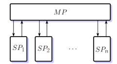
(a) Structure of the classical Dantzig-Wolfe decomposition.

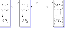
(b) Structure of the Cutting-Plane Consensus algorithm for separable problems.

Figure 3: Comparison of the classical master / subproblem structure of the DW decomposition and the peer-to-peer structure of the Cutting-Plane Consensus algorithm.

The Cutting-Plane Consensus algorithm is applied here to the dual problem and will compute the dual solution to (17), i.e.,

$$\lim_{t\rightarrow\infty}\|\pi^{[i]}(t)-\pi^{*}\|_{2}\rightarrow 0.$$

If all $f_{i}(\cdot)$ in (17) are strictly convex, the solutions of the local subproblems (19) of each processor will converge to the optimal solution, i.e., $\lim_{t\rightarrow\infty}\|\bar{x}_{i}^{[i]}(t)-x_{i}^{*}\|\rightarrow 0,\;\mbox{for\;all\;}i\in V,$ where $x^{*}=[x_{1}^{*},\ldots,x_{n}^{*}]$ is the optimal primal solution to (17), and $\bar{x}_{i}^{[i]}(t)$ is the solution to (19) computed by processor $i$ at time $t$. However, this is not true if some $f_{i}(\cdot)$ are only convex but not strongly convex. Then recovering a primal optimal solution from the dual solution can be done using the method known from DW decomposition. We assume that each processor stores the points at which a constraint is generated, $\bar{x}^{[i]}(\tau)$, where the index $i$ indicates which processor computed at time $\tau$ the point $\bar{x}_{i}(\tau)$ as solution to (19). Define $\bar{G}_{i\tau}:=G_{i}\bar{x}_{i}(\tau)$ and $\bar{f}_{i\tau}:=f_{i}(\bar{x}_{i}(\tau))$. The scalar inequalities of the approximate linear program are all of the form

$$u_{i}-\bar{G}_{i\tau}^{T}\pi\leq\bar{f}_{i\tau}.$$ (21)

One can now formulate the linear programming dual to the approximate program (3). Let $\lambda_{j\tau}\in\mathbb{R}_{\geq 0}$ be the Lagrange multiplier to the constraint (21), the linear programming dual to (3) is a linear program with the following structure:

$$\begin{split}\min_{\lambda_{i\tau}\geq 0}\;&\sum_{i=1}^{n}\sum_{\tau}\bar{f}_{i\tau}\lambda_{i\tau}\\ &\sum_{i=1}^{n}\sum_{\tau}\bar{G}_{i\tau}\lambda_{i\tau}=\mathbf{h},\quad\sum_{\tau}\lambda_{i\tau}=1,\;i\in\{1,\ldots,n\}.\end{split}$$ (22)

We assume in the following that all processors have the same set of constraints (21) as their basis. Please note that this can be achieved by halting the algorithm at some time and running a suitable agreement mechanism, such as the one proposed in [15]. A processor can now reconstruct its component of the solution vector as the convex combination $x_{i}^{*}=\sum_{\tau}\bar{x}_{i}(\tau)\lambda_{i\tau}^{*},$ where $\lambda_{i\tau}^{*}$ solves (22). The resulting solution vector $x^{*}=[x_{1}^{*},\ldots,x_{n}^{*}]$ is globally feasible since $\sum_{i=1}^{n}\sum_{\tau}\bar{G}_{i\tau}\lambda_{i\tau}^{*}=\sum_{i=1}^{n}G_{i}\left(\sum_{\tau}\bar{x}_{i}(\tau)\lambda_{i\tau}^{*}\right)=\sum_{i=1}^{n}G_{i}x_{i}^{*}=\mathbf{h}.$ Additionally, if all processors have computed the globally optimal solution to (18), then the recovered $x_{i}^{*}=\sum_{k}\bar{x}_{i}(\tau)\lambda_{i\tau}$ is also the optimal primal solution to (17). To see this note that strong duality implies that the optimal value of (22) is equivalent to the value of the linear approximate problem (3), which we denote with $f^{*}$. Thus, $f^{*}=\sum_{i=1}^{n}\sum_{\tau=1}f_{i}(\bar{x}_{i}(\tau))\lambda_{i\tau}^{*}$. Convexity of $f_{i}(\cdot)$ and $\sum_{\tau}\lambda_{i\tau}=1$ implies that $f^{*}=\sum_{i=1}^{n}\sum_{\tau}f_{i}(\bar{x}_{i}(\tau))\lambda_{i\tau}^{*}\geq\sum_{i=1}^{n}f_{i}(\sum_{\tau}\bar{x}_{i}(\tau)\lambda_{i\tau}^{*})=:\sum_{i=1}^{n}f_{i}(x_{i}^{*}).$ Since $x^{*}=[x_{1}^{*},\ldots,x_{n}^{*}]$ is a feasible solution it must hold that $\sum_{i=1}^{n}f_{i}(x_{i}^{*})=f^{*}$. Please note that the proposed method requires each processor to store its own local solutions $\bar{x}_{i}^{[i]}(t)$ to (19) generated during the evolution of the algorithm, but does not require that the processors exchange those solutions. For a more explicit discussion on the reconstruction of the feasible solution, we refer the reader to the literature on nonlinear DW-decomposition [3] or our recent paper [17].

Application Example: Distributed Microgrid Control

The previous discussion shows that the Cutting-Plane Consensus algorithm is applicable for many important control problems, such as for example distributed microgrid control. Microgrids are local collections of distributed energy sources, energy storage devices and controllable loads. Most existing control strategies still use a central controller to optimize the operation [40], while for several reasons, detailed, e.g., in [40], distributed control strategies, which do not require to collect all data at a central coordinator, are desirable.

We consider the following optimization model of the microgrid, described recently in [41]. A microgrid consists of several generators, controllable loads, storage devices and a connection to the main grid over which power can be bought or sold. In the following, we use the notational convention that energy generation corresponds to positive variables, while energy consumption corresponds to negative variables. A generator generates power $p_{gen}(t),t\in[0,T]$ within the absolute bounds $\underline{p}(t)\leq p_{gen}(t)\leq\bar{p}(t)$ and the rate constraints $\underline{r}(t)\leq p_{gen}(t+1)-p_{gen}(t)\leq\bar{r}(t)$. The cost to produce power by a generator is modeled as a quadratic function $f_{gen}(t)=\alpha p_{gen}(t)+\beta p^{2}_{gen}(t)$. A storage device can store or release power $p_{st}(t),t\in[0,T]$ within the bounds $-d_{st}\leq p_{st}(t)\leq c_{st}$. The charge level of the storage device is then $q_{st}(t)=q_{st,init}+\sum_{\tau=0}^{t}p_{st}(\tau)$ and must be maintained between $0\leq q_{st}(t)\leq q_{max}$. Note that $p_{st}(t)$ takes negative values if the storage device is charged and positive values if it is discharged. A controllable load has a desired load profile $l_{cl}(t)$ and incorporates a cost if the load is not satisfied, i.e., $f_{cl}(t)=\alpha(l_{cl}(t)-p_{cl}(t))_{+}$, where $(z)_{+}=\max\{0,z\}$. Finally, the microgrid has a single control unit, which coordinates the connection to the main grid and can trade energy. The maximal energy that can be traded is $|p_{tr}|\leq E$. The cost to sell or buy energy is modeled as $f_{tr}=-c^{T}p_{tr}+\gamma^{T}|p_{tr}|$ where $c$ is the price vector and $\gamma$ is a general transaction cost.

The power demand $D(t)$ in the microgrid is predicted over a horizon $T$. The control objective is to minimize the cost of power generation while satisfying the overall demand. This control problem can be directly formulated as in the form (17), with the local objective functions $f_{i}=\sum_{t=0}^{T}f_{i}(t)$, the right-hand side vector of the coupling constraint as the predicted demand $\mathbf{h}=[D(1),\ldots,D(T)]^{T}$ and $\mathcal{X}_{i}$ as the local constraints of each unit.

The Cutting-Plane Consensus algorithm can solve this problem in a distributed way. Note that the objective functions $f_{i}$ considered here are all convex, but not strictly convex. If all objective functions were strictly convex, one could use the distributed Newtons method [9], which has locally a quadratic convergence rate. However, the distributed Newton method does not apply to this problem formulation. The Cutting-Plane Consensus algorithm does not require strict convexity of the cost functions.

We present simulation results for an example set-up with $n=101$ decision units, i.e., 60 generators, 20 storage devices, 20 controllable loads and one connection to the main grid. A random demand is predicted for 15 minute time intervals over a horizon of three hours, based on a constant off-set, a sinusoidal growth and a random component. The algorithm is initialized with each processor computing a basis out of the box-constraint set $\{z:-10^{5}\cdot\boldsymbol{1}\leq z\leq 10^{5}\cdot\boldsymbol{1}\}$, leading to a very high initial objective value.

Figure 4: Trajectories of the scaled maximal optimal value of the linear approximate programs for different $k$-regular communication graphs $\mathcal{G}_{c}$.

Figure 4 shows the largest objective value over all processors, relative to the best solution found as the algorithm is continued to perform. The evolution of the objective value is shown for three different $k$-regular graphs. It can be clearly seen that the convergence speed depends strongly on the structure of the communication graph. The convergence for a network with a 2-regular communication structure is significantly slower than for a network with a higher regular graph. We also want to emphasize the observation that the difference in the convergence speed between $k=8$ and $k=32$ is not as big as the increased communication would let one expect. This shows that the improvement obtained from more communication between the processors becomes smaller with more communication. A good performance of the algorithm can also be obtained with little communication between the processors. Please note that for all communication graphs the Cutting-Plane Consensus algorithm requires only few communication rounds to converge to a fairly good solution. Although the convergence to an exact optimal solution might take more iterations, a good sub-optimal solution can be found after very few communication rounds. This property makes the Cutting-Plane Consensus attractive for control and decision applications.

VIII Discussion and Conclusions

We proposed a framework for distributed convex and robust optimization using a polyhedral approximation method. As a general problem formulation, we consider problems where convex constraint sets are distributed to processors, and the processors have to compute the optimizer of a linear objective function over the intersection of the constraint sets. We proposed the novel Cutting-Plane Consensus algorithm as an asynchronous algorithm performing in peer-to-peer networks. The algorithm is well scalable to large networks in the sense that the amount of data each processor has to store and process is small and independent of the network size.

The appealing property of the considered outer-approximation method lies in the fact that it imposes very little requirements on the structure of the constraint sets. Merely the only requirement is that a cutting-plane oracle exists. We have presented oracles for various formulations of the constraint sets, in particular, inequality and convex uncertain or semi-infinite constraints. Also, we showed that, as the dual problem formulation is considered, also almost separable convex optimization problems can be formulated in the proposed framework. We showed for each of the proposed problem formulations how the cutting-plane oracle can be defined.

Finally, we illustrated that the proposed set-up is of interest for various decision and control problems. These include the localization problem in sensor networks. They include also less obvious problems as, e.g., distributed microgrid control, where the novel algorithm can be applied to the dual problem formulation. In this context we showed that the application of the algorithm to the dual problem has the major advantage that a feasible solution can be found in a fully distributed way even before the algorithm has converged to an optimal solution.

I-A Proofs of Section III

I-A1 Proof of Proposition III.3

The minimal 2-norm solution is the solution to

$$\min_{z,y}\frac{1}{2}z^{T}z,\;\mbox{s.t.}\;A_{H}^{T}z\leq b_{H},\;A_{H}y=c,\;c^{T}z-b_{H}^{T}y=0,\;y\geq 0,$$ (23)

where the constraints represent the linear programming optimality conditions (KKT-conditions). The Lagrangian of (23) can be directly determined to be

$$\mathcal{L}(z,y,u,l,\alpha)=\frac{1}{2}z^{T}z+u^{T}(A_{H}^{T}z-b_{H})+l^{T}(A_{H}y-c)+\alpha(c^{T}z-b_{H}^{T}y),\;y,u\geq 0.$$ (24)

It follows now that $y^{*}=\mbox{arg}\min_{y\geq 0}\;\mathcal{L}(z,y,u,l,\alpha)=0$ if $A_{H}^{T}l-\alpha b_{H}\geq 0.$ From $z^{*}=\mbox{arg}\min_{z}\;,\mathcal{L}(z,y,u,l,\alpha)$ follows that $z^{*}=-A_{H}u-\alpha c.$ The problem (6) stated in the proposition is now $\min_{u\geq 0,l,\alpha}\;-\mathcal{L}(z^{*},y^{*},u,l,\alpha)$. $\hfill\blacksquare$

I-A2 Proof of Lemma III.4

The minimal 2-norm solution $z_{H}^{*}$ is the unique minimizer of

$$\begin{split}\min_{z}\;&\frac{1}{2}\|z\|^{2},\quad\mathrm{s.t.}\;c^{T}z\geq\gamma_{H},\;A_{H}^{T}z\leq b_{H}.\end{split}$$

and satisfies therefore the feasibility conditions $c^{T}z^{*}_{H}=\gamma_{H}$ and $A_{H}^{T}z^{*}_{H}\leq b_{H}.$ Since $z_{H}^{*}$ is an optimal solution, there exist multipliers $\mu^{*}\in\mathbb{R}$ and $\lambda^{*}\in\mathbb{R}^{|H|}_{\geq 0}$, such that the KKT conditions are satisfied, i.e.,

$$z^{*}_{H}-\mu^{*}c+A_{H}\lambda^{*} =0$$ (25)

$$\lambda^{*T}A_{H}^{T}z^{*}_{H}-\lambda^{*T}b_{H} =0.$$ (26)

Since $z^{*}_{H}$ is also a solution to the original linear program (3), there also exists a multiplier vector $y^{*}\in\mathbb{R}^{|H|}_{\geq 0}$ satisfying the linear programming optimality conditions

$$-c+A_{H}y^{*} =0$$ (27)

$$y^{*T}A_{H}^{T}z^{*}_{H}-b^{T}_{H}y^{*} =0.$$ (28)

We have to show now that the existence of $z^{*}_{H},\mu^{*},\lambda^{*}$ and $y^{*}$ imply, for a sufficiently small $\epsilon$, the existence of a multiplier vector $\pi^{*}$ satisfying the optimality conditions of (7), which are

$$\begin{split}-c+\epsilon z^{*}_{H}+A_{H}\pi^{*}&=0\quad\mbox{and}\quad\pi^{*T}A_{H}^{T}z^{*}_{H}-\pi^{*}b_{H}=0.\end{split}$$ (29)

We distinguish now the two cases $\mu^{*}>0$ and $\mu^{*}=0$. First, assume $\mu^{*}>0$. We can multiply (27) with $\frac{t}{\mu^{*}}$, for arbitrary $t\in(0,1]$, and add to this (27), multiplied by $(1-t)$ to obtain

$$\frac{t}{\mu^{*}}z^{*}_{H}-c+A_{H}(\frac{t}{\mu^{*}}\lambda^{*}+(1-t)y^{*})=0.$$ (30)

The same steps can be repeated with (26) and (28) to obtain

$$(\frac{t}{\mu^{*}}\lambda^{*T}+(1-t)y^{*T})(A_{H}^{T}z^{*}_{H}-b_{H})=0.$$ (31)

With (30) and (31), for any $\epsilon\leq\frac{1}{\mu^{*}}$, one can define $t_{\epsilon}=\epsilon\mu^{*}$. Then $\pi^{*}=\frac{t_{\epsilon}}{\mu^{*}}\lambda^{*T}+(1-t_{\epsilon})y^{*T}$ solves (29). In the second case $\mu^{*}=0$, one can pick an arbitrary $\epsilon>0$, multiply (25) (and (26), respectively) with $\epsilon$ and add (27) (or (28), respectively) to obtain $\epsilon z^{*}_{H}-c+A_{H}(\epsilon\lambda^{*}+y^{*})=0$ and $(\epsilon\lambda^{*}+y^{*})(A_{H}^{T}z^{*}_{H}-b_{H})=0.$ Now, $\pi^{*}:=(\epsilon\lambda^{*}+y^{*})$ solves (29). $\hfill\blacksquare$

I-B Proofs of Section IV: Correctness of the Algorithm

Some technical properties of the algorithm are formalized in the following result.

Lemma I.1

Let $z^{[i]}(t)$ be the query point and $B^{[i]}(t)$ the corresponding basis. Let $\mathcal{B}^{[i]}(t)\subset\mathbb{R}^{d}$ be the feasible set induced by $B^{[i]}(t)$. Then,

1. $\mathcal{B}^{[i]}(t)\supset\mathcal{Z}$ for all $i\in\{1\ldots,n\}$ and $t\geq 0$;

2. $\lim_{t\rightarrow\infty}z^{[i]}(t)=\bar{z}$ and $\bar{z}\in\mathcal{Z}$ implies $\bar{z}$ is a minimizer of (1);

3. there exists $\underline{\epsilon}>0$ such that for all $i\in\{1,\ldots,n\}$ and all $t\geq 0$, the query points $z^{[i]}(t)$ maximize the objective function

   $$J_{\epsilon}(z):=c^{T}z-\frac{\epsilon}{2}\|z\|^{2}_{2}$$

   over the set of constraints $B^{[i]}(t)\cup Y^{[i]}(t)$ (as defined in (S2)) for all $\epsilon\in[0,\underline{\epsilon}]$;

4. $J_{\underline{\epsilon}}(z^{[i]}(t+1))\leq J_{\underline{\epsilon}}(z^{[i]}(t))$ for all $i\in\{1,\ldots,n\}$ and all $t\geq 0$;

5. if $\mathcal{G}_{c}$ is a strongly connected static graph, then $J_{\underline{\epsilon}}(z^{[j]}(t+\operatorname{diam}(\mathcal{G}_{c})))\leq J_{\underline{\epsilon}}(z^{[i]}(t))$ for all $i,j\in\{1,\ldots,n\}$ and all $t\geq 0$.

Proof:

To see (i), note that any cut $h_{k}$ generated by the oracle of processor $i$, $\operatorname{ORC}(\cdot,\mathcal{Z}_{i})$ is such that the half-space $h_{k}$ contains $\mathcal{Z}_{i}$, and in particular $h_{k}$ contains $\mathcal{Z}=\bigcap_{i=1}^{n}\mathcal{Z}_{i}$. Thus any collection of cuts $H=\bigcup_{k}h_{k}$, generated by arbitrary processors is such that $\mathcal{H}\supset\bigcap_{i=1}^{n}\mathcal{Z}_{i}=\mathcal{Z}$, and in particular $\mathcal{B}^{[i]}(t)\supset\mathcal{Z}$. The claim (ii) follows since $z^{[i]}(t)$ is computed as a maximizer of the linear cost $c^{T}z$ over the collection of cutting-planes $H^{[i]}_{tmp}(t)$. The induced polyhedron is such that $\mathcal{H}_{tmp}^{[i]}(t)\supset\mathcal{Z}$. Therefore, we can conclude that $c^{T}z^{[i]}(t)\geq c^{T}z^{*}$, where $z^{*}$ is an optimizer of (1). By continuity of the linear objective function, we have that $c^{T}\bar{z}\geq c^{T}z^{*}$ On the other hand, $c^{T}z\leq c^{T}z^{*}$ for all $z\in\mathcal{Z}$. This proves the statement. The statement (iii) follows from Lemma III.4. For any approximate program defined by processor $i$ at time $t$, there exists a constant $\bar{\epsilon}_{it}>0$ such that $z^{[i]}(t)$ is the unique maximizer of the family of strictly concave objective functions $J_{\epsilon}(z):=c^{T}z-\frac{\epsilon}{2}\|z\|^{2},\quad\epsilon\in[0,\bar{\epsilon}_{it}],$ over the set of constraints $B^{[i]}(t)\cup Y^{[i]}(t)$. One can now always find $\underline{\epsilon}>0$ such that $\underline{\epsilon}\leq\bar{\epsilon}_{it}$ for all $i\in\{1,\ldots,n\}$ and $t\geq 0$. To see claim (iv), note that adding cutting-planes, either by receiving them from neighbors (S2) or by generating them with the oracle (S3), can only decrease the value of the strictly concave objective function $J_{\underline{\epsilon}}(\cdot)$ and the basis computation in (S4) keeps, by its definition, the value of $J_{\underline{\epsilon}}(\cdot)$ constant. Finally, (v) can be seen as follows. Starting at any time $t$ at some processor $i$, at time $t+1$ all processors in $l\in\mathcal{N}_{I}(i,t)$ received the basis of processor $i$, and compute a query point that satisfies $J_{\underline{\epsilon}}(z^{[l]}(t+1))\leq J_{\underline{\epsilon}}(z^{[i]}(t))$ for all $l\in\mathcal{N}_{I}(i,t)$. This argument can be repeatedly applied to see that, in the static, strongly connected communication graph $\mathcal{G}_{c}$, at least after $\operatorname{diam}(\mathcal{G}_{c})$ iterations, all processors in the network have an objective value smaller than $J_{\underline{\epsilon}}(z^{[i]}(t))$. ∎

Next we present the proof of Lemma IV.1, Lemma IV.2, and Theorem IV.3. The following proofs use the parameterized cost function $J_{\underline{\epsilon}}(\cdot)$. However, for the clarity of presentation we will simplify our notation in the following proofs and write simply $J(\cdot)$ instead of $J_{\underline{\epsilon}}(\cdot)$.

I-B1 Proof of Lemma IV.1

All $z^{[i]}(t)$ are computed as maximizers of the common strictly concave objective function $J(\cdot)$ (Lemma I.1 (iii)) and $J(\cdot)$ is monotonically non-increasing over the sequence of query points computed by a processor (Lemma I.1 (iv)). Any sequence $\{J(z^{[i]}(t))\}_{t\geq 0}$, $i\in\{1,\ldots,n\}$, has therefore a limit point, i.e., $\lim_{t\rightarrow\infty}J(z^{[i]}(t))\rightarrow\bar{J}^{[i]}$. Since the sequence is convergent, it holds that $\lim_{t\rightarrow\infty}\left(J(z^{[i]}(t))-J(z^{[i]}(t+1))\right)\rightarrow 0.$ By strict concavity of $J(\cdot)$ follows that $J(z^{[i]}(t))-J(z^{[i]}(t+1))>\sigma\|z^{[i]}(t)-z^{[i]}(t+1)\|^{2}_{2}$ for some $\sigma>0$. Consequently, $\lim_{t\rightarrow\infty}\|z^{[i]}(t)-z^{[i]}(t+1)\|_{2}\rightarrow 0$ and the sequence of query points has a limit point, i.e., $\lim_{t\rightarrow\infty}\|z^{[i]}(t)-\bar{z}^{[i]}\|_{2}\rightarrow 0$. Suppose now, to get a contradiction, that $\bar{z}^{[i]}\notin\mathcal{Z}_{i}$. Then there exists $\delta>0$ such that all $z$ satisfying $\|z-\bar{z}^{[i]}\|_{2}<\delta$ are not contained in $\mathcal{Z}_{i}$. Since $\lim_{t\rightarrow\infty}\|z^{[i]}(t)-\bar{z}^{[i]}\|_{2}\rightarrow 0$, there exists a time instant $T_{\delta}$ such that $\|z^{[i]}(t)-\bar{z}^{[i]}\|_{2}<\delta$ for all $t\geq T_{\delta}$, and thus $z^{[i]}(t)\notin\mathcal{Z}_{i}$ for $t\geq T_{\delta}$. But now, for all $t\geq T_{\delta}$ the oracle $\operatorname{ORC}(z^{[i]}(t),\mathcal{Z}_{i})$ will generate a cutting-plane according to (2), cutting off $z^{[i]}(t)$. According to (2), it must hold that $a^{T}(z^{[i]}(t))z^{[i]}(t)-b(z^{[i]})=s(z^{[i]}(t))>0$ and $a^{T}(z^{[i]}(t))z^{[i]}(t+1)-b(z^{[i]})\leq 0$. This implies that $a^{T}(z^{[i]}(t))\left(z^{[i]}(t)-z^{[i]}(t+1)\right)\geq s(z^{[i]}(t))$ and consequently $\|z^{[i]}(t)-z^{[i]}(t+1)\|_{2}\geq(\|a(z^{[i]}(t))\|_{2})^{-1}s(z^{[i]}(t)).$ By Assumption III.1 (i) holds $\|a(z^{[i]}(t))\|_{2}<\infty$ and thus $\lim_{t\rightarrow\infty}s(z^{[i]}(t))\rightarrow 0$. As a consequence of Ass. III.1 (ii) follows directly that $\bar{z}^{[i]}\in\mathcal{Z}_{i}$, providing the contradiction. $\hfill\blacksquare$

I-B2 Proof of Lemma IV.2:

Let $\bar{J}^{[i]}:=J(\bar{z}^{[i]})$ be the objective value of the limit point $\bar{z}^{[i]}$ of the sequence $\{z^{[i]}(t)\}_{t\geq 0}$ computed by processor $i$. We show first that the limiting objective values $\bar{J}^{[i]}$ are identical for all processors. Suppose by contradiction that there exist two processors, say $i$ and $j$, such that $\bar{J}^{[i]}<\bar{J}^{[j]}.$ Pick now $\delta_{0}>0$ such that $\bar{J}^{[j]}-\bar{J}^{[i]}>\delta_{0}.$ The sequences $\{J(z^{[i]}(t))\}_{t\geq 0}$ and $\{J(z^{[j]}(t))\}_{t\geq 0}$ are monotonically increasing and convergent. Thus, for every $\delta>0$ there exists a time $T_{\delta}$ such that for all $t\geq T_{\delta}$, $J(z^{[i]}(t))-\bar{J}^{[i]}\leq\delta$ and $J(z^{[j]}(t))-\bar{J}^{[j]}\leq\delta.$ This implies that there exists $T_{\delta_{0}}$ such that for all $t\geq T_{\delta_{0}}$,

$$J(z^{[i]}(t))\leq\delta_{0}+\bar{J}^{[i]}<\bar{J}^{[j]}.$$

Additionally, since the objective functions are non-increasing, it follows that for any time instant $t^{\prime}\geq 0$, $J(z^{[j]}(t^{\prime}))\geq\bar{J}^{[j]}$. Thus, for all $t\geq T_{\delta_{0}}$ and all $t^{\prime}\geq 0$,

$$J(z^{[i]}(t))<J(z^{[j]}(t^{\prime})).$$ (32)

Pick now $t_{0}\geq T_{\delta_{0}}$. For all $\tau\geq 0$ define now an index set $I_{\tau}$ as follows: Set $I_{0}=\{i\}$ and for any $\tau\geq 0$ define $I_{\tau}$ by adding to $I_{\tau-1}$ all indices $k$ for which there exist some $l\in I_{\tau-1}$ such that $(k,l)\in E(t_{0}+\tau)$. Since, by assumption $\mathcal{G}_{c}^{\infty}(t_{0})$ is strongly connected, the set $I_{\tau}$ will eventually include all indices $1,\ldots,n$, and in particular there is $\tau^{*}$ such that $j\in I_{\tau^{*}}$. The algorithm is such that for all $l\in I_{\tau}$, $J(z^{[l]}(t_{0}+\tau))\leq J(z^{[i]}(t_{0}))$ and thus

$$J(z^{[j]}(t_{0}+\tau^{*}))\leq J(z^{[i]}(t_{0})).$$ (33)

But (33) contradicts (32), proving that $\bar{J}^{[i]}=\bar{J}^{[2]}=\cdots=\bar{J}^{[n]}=:\bar{J}.$ Thus, it must hold that for all $i,j\in\{1,\ldots,n\}$, $\lim_{t\rightarrow\infty}|J(z^{[i]}(t))-J(z^{j}(t))|\rightarrow 0$. From the strict concavity of $J(\cdot)$ follows that $|J(z^{[i]}(t))-J(z^{[j]}(t))|>\sigma\|z^{[i]}(t)-z^{[j]}(t)\|_{2}^{2},$ for some $\sigma>0$. Therefore, $\lim_{t\rightarrow\infty}\|z^{[i]}(t)-z^{[j]}(t)\|_{2}\rightarrow\infty$, which proves the theorem. $\hfill\blacksquare$

I-B3 Proof of Theorem IV.3

It follows from Lemma IV.2 that the query points of all processors converge to the same query point, i.e., $\bar{z}^{[i]}=\bar{z}$ for all processors $i$. Now, we can conclude from Lemma IV.1 that $\bar{z}\in\mathcal{Z}_{i}$ for all $i$ and thus $\bar{z}\in\mathcal{Z}$. It follows now from Lemma I.1, part (ii), that $\bar{z}$ is an optimal solution to (1). It remains to show that $\bar{z}$ is the optimal solution with minimal 2-norm. Let $z^{*}$ be the optimal solution with minimal 2-norm. Then there exists an $\epsilon>0$ such that the parameterized objective function satisfies $J_{\epsilon}(z^{*})>J_{\epsilon}(z)$ for all $z\in\mathcal{Z}$ and $J_{\epsilon}(z^{[i]}(t))\geq J_{\epsilon}(z^{*})$ for all $t$. With the same argumentation used for Lemma I.1, part (ii), we conclude that $\bar{z}$ is the unique solution maximizing $J_{\epsilon}(\cdot)$ over $\mathcal{Z}$, i.e., $\bar{z}$ is the optimal solution to (1) with minimal 2-norm. $\hfill\blacksquare$

References

- [1] F. Bullo, J. Cortés, and S. Martínez, Distributed Control of Robotic Networks, ser. Applied Mathematics Series. Princeton University Press, 2009. [Online]. Available: http://coordinationbook.info
- [2] D. P. Bertsekas and J. N. Tsitsiklis, Parallel and Distributed Computations: Numerical Methods. Belmont, Massachusetts: Athena Scientific, 1997.
- [3] L. S. Lasdon, Optimization Theory for Large Scale Systems. Courier Dover Publications, 2002.
- [4] J. Tsitsiklis, D. Bertsekas, and M. Athans, “Distributed asynchronous deterministic and stochastic gradient optimization algorithms,” IEEE Transactions on Automatic Control, vol. 31, no. 9, pp. 803–812, 1986.
- [5] A. Nedic and A. Ozdaglar, “Distributed subgradient methods for multi-agent optimization,” IEEE Transactions on Automatic Control, vol. 54, no. 1, pp. 48–61, 2009.
- [6] S. H. Low and D. E. Lapsley, “Optimization flow control - i: Basic algorithm and convergence,” IEEE/ACM Transactions on Networking, vol. 7, no. 6, pp. 861–874, 1999.
- [7] S. H. Low, F. Paganini, and J. C. Doyle, “Internet congestion control,” IEEE Control Systems Magazine, vol. 22, no. 1, pp. 28 – 43, 2002.
- [8] A. Nedic, A. Ozdaglar, and P. A. Parrilo, “Constrained consensus and optimization in multi-agent networks,” IEEE Transactions on Automatic Control, vol. 55, no. 4, pp. 922–938, 2010.
- [9] M. Zargham, A. Ribeiro, A. Jadbabaie, and A. Ozdaglar, “Accelerated dual descent for network optimization,” IEEE Transactions on Automatic Control, 2011, submitted (Nov. 2011).
- [10] M. Zargham, A. Ribeiro, A. Ozdaglar, and A. Jadbabaie, “Accelerated dual descent for network optimization,” in Proc. American Control Conference, San Francisco, CA, June 2011, pp. 266–2668.
- [11] F. Zanella, D. Varagnolo, A. Cenedese, P. Gianluigi, and L. Scenato, “Newton-raphson consensus for distributed convex optimization,” in Proc. 50th IEEE Conf. on Decision and Control, Orlando, Florida, December 2011, pp. 5917 – 5922.
- [12] I. D. Schizas, A. Ribeiro, and G. B. Giannakis, “Consensus in ad hoc WSNs with noisy links - part I: Distributed estimation of deterministic signals,” IEEE Transactions on Signal Processing, vol. 56, no. 1, pp. 350 – 364, 2008.
- [13] S. Boyd, N. Parikh, E. Chu, B. Peleato, and J. Eckstein, “Distributed optimization and statistical learning via alternating direction method of multipliers,” Foundations and Trends in Machine Learning, vol. 3, no. 1, pp. 1 – 122, 2010.
- [14] G. Notarstefano and F. Bullo, “Network abstract linear programming with application to minimum-time formation control,” in IEEE Conference on Decision and Control, New Orleans, USA, 2007, pp. 927–932.
- [15] ——, “Distributed abstract optimization via constraints consensus: Theory and applications,” IEEE Transactions on Automatic Control, vol. 56, no. 10, pp. 2247–2261, 2011.
- [16] M. Bürger, G. Notarstefano, F. Bullo, and F. Allgöwer, “A distributed simplex algorithm for degenerate linear programs and multi-agent assignments,” Automatica, vol. 48, no. 9, pp. 2298 – 2304, 2012.
- [17] M. Bürger, G. Notarstefano, and F. Allgöwer, “Locally constrained decision making via two-stage distributed simplex,” in Proc. IEEE Conference on Decision and Control, European Control Conference, Orlando, Dec. 2011, pp. 5911 – 5916.
- [18] ——, “Distributed robust optimization via cutting-plane consensus,” in Proc. IEEE Conference on Decision and Control, Maui, Hawaii, Dec. 2012.
- [19] G. Dantzig and P. Wolfe, “The decomposition algorithm for linear programs,” Econometrica, vol. 29, no. 4, pp. 767 – 778, 1961.
- [20] B. C. Eaves and W. I. Zangwill, “Generalized cutting plane algorithms,” SIAM Journal of Control and Optimization, vol. 9, no. 4, pp. 529 – 542, 1971.
- [21] O. L. Mangasarian, “Least-norm linear programming solution as an unconstrained optimization problem,” Journal of Mathematical Analysis and Applications, vol. 92, pp. 240 – 251, 1983.
- [22] Y.-B. Zhao and D. Li, “Locating the least 2-norm solution of linear programs via a path-following method,” SIAM Journal on Optimization, vol. 12, no. 4, pp. 893 – 912, 2002.
- [23] O. L. Mangasarian and R. R. Meyer, “Nonlinear perturbation of linear programs,” SIAM Journal on Optimization, vol. 17, no. 6, pp. 745 – 752, 1979.
- [24] J. E. Kelley, “The cutting plane method for solving convex programs,” SIAM Journal on Applied Mathematics, vol. 8, pp. 703 – 712, 1960.
- [25] C. Scherer and S. Weiland, “Linear matrix inequalities in control,” Delft Center for Systems and Control, Delft University of Technology, The Netherlands, Tech. Rep., 2004.
- [26] K. Krishnan and J. Mitchell, “A unifying framework for several cutting plane methods for semidefinite programming,” Optimization Methods and Software, vol. 21, pp. 57 – 74, 2006.
- [27] H. Konno, N. Kawadai, and H. Tuy, “Cutting-plane algorithms for nonlinear semi-definite programming problems with applications,” Journal of Global Optimization, vol. 25, pp. 141 – 155, 2003.
- [28] J. Bachrach and C. Taylor, Handbook of sensor networks. John Wiley and Sons, Inc., 2005, ch. Localization in Sensor Networks, pp. 277–310.
- [29] L. Doherty, K. Pister, and L. E. Ghaoui, “Convex position estimation in wireless sensor networks,” in 20th IEEE Conference on Computer Communications Societies, vol. 3, 2001, pp. 1655 –1663.
- [30] M. Lopez and G. Still, “Semi-infinite programming,” European Journal of Operational Research, vol. 180, pp. 491–518, 2007.
- [31] A. Ben-Tal, L. E. Ghaoui, and A. Nemirovski, Robust Optimization. Princeton University Press, 2009.
- [32] G. Calafiore, “Random convex programs,” SIAM Journal on Optimization, vol. 20, no. 6, pp. 3427 – 3464, 2010.
- [33] L. Carlone, V. Srivastava, F. Bullo, and G. C. Calafiore, “Distributed random convex programming via constraints consensus,” SIAM Journal of Control and Optimization, Jul. 2012, submitted.
- [34] R. Reemtsen, “Some outer approximation methods for semi-infinite optimization problems,” Journal of Computational and Applied Mathematics, vol. 53, pp. 87 – 108, 1994.
- [35] A. Mutapcic and S. Boyd, “Cutting-set methods for robust convex optimization with pessimizing oracles,” Optimization Methods and Software, vol. 24, pp. 381– 406, 2009.
- [36] K. Yang, Y. Wu, J. Huang, X. Wang, and S. Verdu, “Distributed robust optimization for communication networks,” in INFOCOM 2008. The 27th Conference on Computer Communications. IEEE, 2008, pp. 1157–1165.
- [37] A. Ben-Tal and A. Nemirovski, “Robust solutions of uncertain linear programs,” Operations Research Letters, vol. 25, pp. 1–13, 1999.
- [38] J. R. Dunham, D. G. Kelly, and J. W. Tolle, “Some experimental results concerning the expected number of pivots for solving randomly generated linear programs,” University of North Carolina and Chapel Hill, Tech. Rep. 77-16, 1977.
- [39] A. Olshevsky and J. Tsistiklis, “Convergence speed in distributed consensus and averaging,” SIAM Journal of Control and Optimization, vol. 48, no. 1, pp. 33–55, 2009.
- [40] R. Zamora and A. K. Srivastava, “Controls for microgrids with storage: Review, challenges and research needs,” Renewable and Sustainable Energy Reviews, vol. 14, pp. 2009–2018, 2010.
- [41] M. Kraning, E. Chu, J. Lavaei, and S. Boyd, “Message passing for dynamic network energy management,” Stanford University, Tech. Rep., 2012. [Online]. Available: http://www.stanford.edu/ boyd/papers/pdf/decen_dyn_opt.pdf