A Truncated partial wave analysis of a complete experiment for photoproduction of two pseudoscalar mesons on a nucleon

Abstract

A truncated partial wave analysis for the photoproduction of two pseudoscalar mesons on a nucleon is discussed with respect to the determination of a complete set of observables. For the selection of such a set we have applied a criterion previously developed for photo- and electrodisintegration of a deuteron, which allows one to find a ’minimal’ set of observables for determining the partial wave amplitudes up to possible discrete ambiguities. The question of resolving the remaining ambiguities by invoking additional observables is discussed for the simplest case, when the partial wave expansion is truncated at the lowest total angular momentum of the final state $J_{max}=1/2$. The resulting ’fully’ complete set, allowing an unambiguous determination of the partial wave amplitudes, is presented.

I Introduction

Photoproduction of two pseudoscalars on nucleons have been studied rather intensively during the last two decades. At present a large amount of experimental data, in particular for $\pi^{0}\pi^{0}$ and $\pi^{0}\eta$ channels, have been collected and some new experiments on polarization observables for these reactions are planned. The interpretation of the data within different models has allowed one to qualitatively understand the major mechanisms of these processes. At the same time, although the general agreement of the various calculations with the measured cross sections is reasonable, significant qualitative differences between these models exist. Some of them were already discussed, for example in Ref. Kashev2pi0 .

One reason for these differences between theoretical results is that the standard approach, based on the isobar model, appears to have reached certain limitations. Probably its weakest point is that the corresponding formalism depends on a specific assumption about the dynamics of the production process. Within the isobar model approach one assumes that the two-body discontinuity in the reaction matrix coming from the interaction in the two-body subsystems in the final state may be approximated by resonance terms (usually taken in the Breit-Wigner form). In other words, it is assumed that the final three-particle state is produced via intermediate formation of quasi two-body states containing meson-nucleon and meson-meson isobars.

In order to achieve a significant improvement of present theoretical models one has to eliminate as much as possible the mentioned model dependencies from the formal description of these reactions. In this respect, an ideal tool for the investigation of the reaction dynamics is an analysis of a complete experiment within a given model, based on the fundamental principles of rotation and parity invariance. It is clear that for the photoproduction of two mesons this task is considerably more complicated in comparison to the photoproduction of a single meson. Firstly, in the case of three particles in the final state, the amplitudes depend on five kinematical variables, so that for their determination accurate measurements of five-dimensional distributions are needed. Secondly, contrary to the single meson case, a complete set contains a considerably larger number of observables. Indeed, if two mesons are produced, the property of parity conservation does not allow one to reduce the number of independent amplitudes. Therefore, in order to determine all eight complex amplitudes up to an overall phase one needs at least 15 observables. As was shown by Roberts and Oed Roberts , a complete set includes not only single and double but also triple polarization observables. The latter is especially disappointing since it requires the implementation of complicated measurements at a high level of accuracy.

At the same time, as was noted in Refs. Workman and Tiat , arbitrariness in the overall phase at each point of the phase space does not allow one to find the multipole amplitudes, which are obviously needed for a nucleon resonance analysis. Therefore, if one searches for resonances or, more generally, for states with definite spin and parity $J^{P}$, it is more reasonable (and probably less complicated) to adopt a truncated partial wave expansion up to a maximal total angular momentum $J_{max}$ and to study instead of the spin or helicity amplitudes the partial wave amplitudes. In this case, as a rule, a lower number of polarization observables is needed. As is discussed in Refs. Tiat ; Grush ; Omel for $\gamma N\to\pi^{0}N$, in order to determine (up to an overall phase) the multipoles $E_{0+}$, $E_{1+}$, and $M_{1\pm}$ which are important in the first resonance region, already a set of single polarization observables with an additional measurement of only one of the double polarization observables (for example, $F$- or $G$-asymmetry) is sufficient.

For a partial wave analysis we firstly need a convenient and model independent form of the partial wave decomposition of the reaction amplitude. As already noted above, the isobar model does not meet this requirement, since it depends on specific assumptions about the reaction dynamics. Therefore, we adopt in the present paper the formalism developed in Ref. FiA12 . Here a special coordinate frame is used in which the $z$-axis is chosen along the normal to the plane spanned by the momenta of the final particles in the overall center-of-mass frame. In this case one can choose as independent kinematical variables the energies of two of the three final particles and three angles, determining the orientation of the final state plane with respect to the photon beam (one of the angles corresponds to the rotation around the normal). Then the amplitude for a given total angular momentum $J$ of the final state and its projection $M$ on the $z$-axis is obtained by an expansion of the helicity amplitudes over a set of Wigner functions. In Ref. Kashev2pi0 this approach was applied successfully to the analysis of the unpolarized differential cross section for the photoproduction of $\pi^{0}\pi^{0}$ pairs.

The second important question is what is an optimal choice of the observables needed for the determination of the partial wave amplitudes. While for the determination of $n$ complex quantities (up to an overall phase factor) only $2n-1$ real parameters are needed, the total number of linearly independent observables (or, more generally, the number of bilinear hermitian forms of the amplitudes) is $n^{2}$. This means that there exist also nonlinear dependencies between the observables, so that not any subset of $2n-1$ observables may form a complete set from which the $2n-1$ real parameters can be deduced.

Thus the question is how to select out of this set of $n^{2}$ observables a subset of $2n-1$ independent observables. In the present paper we describe a method which may be used to single out a minimal set of independent observables. The criterion, which underlies the method, was originally developed for deuteron photo- and electrodisintegration in Refs. ArLeiTom ; ArLeiTomFBS . An additional very important question concerns possible discrete ambiguities, which naturally can appear since the extraction of the amplitudes implies a solution of a set of quadratic equations. To resolve these ambiguities we adopt for our truncated partial wave analysis an additional criterion, which was used in Ref. Tabakin for the spin amplitude analysis of single meson photoproduction.

First, we present in the next section a brief review of the formalism developed in Ref. FiA12 . Then we give in Sec. III an example of the method of how to find a complete set of observables for the simplest case, when only partial waves with $J=1/2$ and both parities are included. In Sect. IV we summarize our results and give an outlook on future developments. Some details are collected in two appendices.

II Formal developments

For the theoretical description we choose the overall c.m. system. The four-momenta of incoming photon, outgoing mesons, and final nucleon are denoted by $(\omega_{\gamma},\vec{k}\,)$, $(\omega_{1},\vec{q}_{1}\,)$, $(\omega_{2},\vec{q}_{2}\,)$, and $(E,\vec{p}\,)$, respectively. We consider within this system two right-handed orthogonal coordinate systems: (i) one associated with the incoming photon called $K_{\gamma}$ with $z$-axis along the photon momentum and $x$-axis arbitrary, and (ii) the so-called “rigid body” system $K_{fs}$, associated with the final state plane spanned by the final three particles, in which the $z$-axis is taken to be the normal to this plane and parallel to $\vec{p}\times\vec{q}_{1}$. Thus the $x$- and $y$-axes are in the final scattering plane (see Fig. 1). The transformation from $K_{fs}$ to $K_{\gamma}$ is given by a rotation through Euler angles $(\phi,\theta,0)$. Thus relative to $K_{fs}$ the photon momentum $\vec{k}$ has the spherical angles $\Omega_{\gamma}=(\theta_{\gamma},\phi_{\gamma})$.

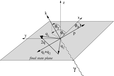
Figure 1: Definition of the coordinate system in the c.m. system.

For the $T$-matrix we had derived in Ref. FiA12 the following expression expanding the final state into partial waves

$$T_{\nu\lambda\mu}(\phi_{p},\omega_{1},\omega_{2},\Omega_{\gamma}) = e^{-i\nu\phi_{p}}\sum\limits_{JM_{J}}t^{JM_{J}}_{\nu\lambda\mu}(\omega_{1},\omega_{2})\,D^{J}_{M_{J}\,\lambda-\mu}(R_{\gamma p})\,,$$ (1)

where $J$ and $M_{J}$ denote respectively the total angular momentum of the partial wave and its projection on the normal to the final state plane. The rotation matrix $D^{J}_{M^{\prime}M}$ is taken in the convention of Rose Ros57 with argument $R_{\gamma p}=(\phi_{\gamma p},\theta_{\gamma},-\phi_{\gamma})$ and $\phi_{\gamma p}=\phi_{\gamma}-\phi_{p}$. The helicities of photon and initial and final nucleons are denoted by $\lambda$, $\mu$, and $\nu$, respectively. As independent variables we had chosen besides the photon angles $\Omega_{\gamma}=(\theta_{\gamma},\phi_{\gamma})$ and the proton angle $\phi_{p}$ in the final state plane, the energies of the two final mesons $\omega_{1}$ and $\omega_{2}$. The latter two determine the relative angle $\phi_{qp}=\phi_{q}-\phi_{p}$ between the momentum of the final proton and the relative momentum $\vec{q}=(\vec{q}_{1}-\vec{q}_{2})/2$ of the two mesons according to

$$\cos\phi_{qp}=\frac{1}{2qp}(\omega_{2}^{2}-\omega_{1}^{2}-M_{2}^{2}+M_{1}^{2})\,,$$ (2)

with the final nucleon momentum

$$p=|\vec{p}\,|=\sqrt{(W-\omega_{1}-\omega_{2})^{2}-M_{N}^{2}}\,,$$ (3)

where $W$ denotes the invariant total energy, and the relative momentum $q$ of the two mesons is determined by

$$q^{2}=\frac{1}{2}(\omega_{1}^{2}+\omega_{2}^{2}-M_{1}^{2}-M_{2}^{2})-\frac{p^{2}}{4}\,.$$ (4)

In the foregoing equations the masses of the nucleon and the two mesons are denoted by $M_{N}$, $M_{1}$ and $M_{2}$, respectively.

The expression in Eq. (1) is obtained by making use of rotation and inversion invariance (that is angular momentum and parity conservation) and is therefore completely general. The final partial wave is taken in the form $|qp;\,((l_{p}\frac{1}{2})j_{p}l_{q})JM_{J}\rangle^{(-)}$ where $l_{p}$ and $l_{q}$ denote the angular momenta of nucleon and meson pair, respectively.

The contribution of the final partial wave to the reaction amplitude is given by

$$t^{JM_{J}}_{\nu\lambda\mu}(\omega_{1},\omega_{2}) = t^{JM_{J}}_{\nu\lambda\mu}(\phi_{qp})$$ (9)

$$= \sum_{l_{p}j_{p}m_{p}L}\left(\begin{array}[]{ccc}l_{p}&\frac{1}{2}&j_{p}\cr 0&\nu&-\nu\cr\end{array}\right)\left(\begin{array}[]{ccc}J&L&\frac{1}{2}\cr\mu-\lambda&\lambda&-\mu\cr\end{array}\right)d^{j_{p}}_{\nu\,m_{p}}(\pi/2)\,e^{i(M_{J}-m_{p})\phi_{qp}}\,{\cal O}^{\lambda LJ}_{M_{J}}(l_{p}j_{p}m_{p})\,,$$

with

$${\cal O}^{\lambda LJ}_{M_{J}}(l_{p}j_{p}m_{p}) = \frac{(-1)^{1+J}\widehat{J}}{2\sqrt{2\pi}}\sum_{l_{q}m_{q}}i^{L}(-1)^{l_{p}+j_{p}+l_{q}}\,\widehat{l}_{p}\,\widehat{j}_{p}\,\widehat{l}_{q}\,\widehat{L}\,d^{l_{q}}_{0\,m_{q}}(\pi/2)$$ (10)

$$\times\left(\begin{matrix}j_{p}&l_{q}&J\cr m_{p}&m_{q}&-M_{J}\cr\end{matrix}\right)\langle p\,q;\big{(}(l_{p}\frac{1}{2})j_{p}l_{q}\big{)}J||{\cal O}^{\lambda L}||\frac{1}{2}\rangle\,,$$

where $\hat{l}=\sqrt{2l+1}$ and ${\cal O}^{\lambda L}$ denotes the electromagnetic multipole operator with electric and magnetic contributions

$${\cal O}^{\lambda L}_{M} = E_{M}^{L}+\lambda M_{M}^{L}\,.$$ (11)

The amplitudes $t_{\nu\lambda\mu}^{JM_{J}}$ obey the following symmetry property which follows from parity conservation (see Ref. FiA12 , one should note a misprint in the phase)

$$t_{-\nu-\lambda-\mu}^{JM_{J}}(\phi_{qp})=(-1)^{\nu-M_{J}}t_{\nu\lambda\mu}^{J-M_{J}}(-\phi_{qp})\,.$$ (12)

The interchange $\phi_{qp}\leftrightarrow-\phi_{qp}$ corresponds to the interchange $(\omega_{1},M_{1})\leftrightarrow(\omega_{2},M_{2})$, see Eq. (2) through (4). Therefore, parity conservation does not reduce the number of independent amplitudes in this case in contrast to single meson production as already noted in Ref. Roberts . However, in a more general sense this relation allows one to reduce the number of independent amplitudes. Namely, provided that the amplitude $t_{\nu\lambda\mu}^{JM_{J}}$ is known in the whole region of the Dalitz plot $(\omega_{1},\omega_{2})$ the amplitude $t_{-\nu-\lambda-\mu}^{J-M_{J}}$ can be obtained using the symmetry relation of Eq. (12). Thus in this more general sense one has $4(2J+1)$ independent amplitudes for a given $J$, except for $J=1/2$ for which this number is reduced to $2(2J+1)=4$ because of an additional requirement $\lambda-\mu\leq J$, coming from angular momentum conservation.

As shown in Appendix A, one can separate the contributions of those final states with positive parity from those of negative one according to

$$t^{JM_{J}}_{\nu\lambda\mu}=(-)^{\delta_{\nu-\frac{1}{2}}(\frac{1}{2}+M)}(t^{JM_{J}\,+}_{\lambda\mu}+2\nu\,t^{JM_{J}\,-}_{\lambda\mu})\,,$$ (13)

where

$$t^{JM_{J}\,\pm}_{\lambda\mu}=\frac{1}{2}\Big{(}t^{JM_{J}}_{1/2\lambda\mu}\pm(-)^{\frac{1}{2}+M_{J}}t^{JM_{J}}_{-1/2\lambda\mu}\Big{)}\,.$$ (14)

An interesting consequence of Eq. (13) is that the bilinear expression $t^{J^{\prime}M^{\prime}_{J}*}_{\nu^{\prime}\lambda^{\prime}\mu^{\prime}}t^{JM_{J}}_{\nu\lambda\mu}$ with $\nu^{\prime}=\nu$ is invariant under the transformation (parity exchange)

$$t_{\lambda\mu}^{JM_{J}+}\leftrightarrow t_{\lambda\mu}^{JM_{J}-}\,,$$ (15)

which, as follows from Eq. (14), is equivalent to the transformation of the matrices $t^{JM_{J}}_{\nu\lambda\mu}$

$$t^{JM_{J}}_{\nu\lambda\mu}\rightarrow 2\nu\,t^{JM_{J}}_{\nu\lambda\mu}\,.$$ (16)

Indeed, one finds successively (note $2\nu=\pm 1$)

$$t^{J^{\prime}M^{\prime}_{J}*}_{\nu\lambda^{\prime}\mu^{\prime}}t^{JM_{J}}_{\nu\lambda\mu} = (t^{J^{\prime}M_{J}^{\prime}\,+}_{\lambda^{\prime}\mu^{\prime}}+2\nu\,t^{J^{\prime}M^{\prime}_{J}\,-}_{\lambda^{\prime}\mu^{\prime}})^{*}(t^{JM_{J}\,+}_{\lambda\mu}+2\nu\,t^{JM_{J}\,-}_{\lambda\mu})$$ (17)

$$= (2\nu\,t^{J^{\prime}M_{J}^{\prime}\,+}_{\lambda^{\prime}\mu^{\prime}}+t^{J^{\prime}M^{\prime}_{J}\,-}_{\lambda^{\prime}\mu^{\prime}})^{*}(2\nu\,t^{JM_{J}\,+}_{\lambda\mu}+t^{JM_{J}\,-}_{\lambda\mu})$$

$$\Rightarrow (2\nu\,t^{J^{\prime}M^{\prime}_{J}\,-}_{\lambda^{\prime}\mu^{\prime}}+t^{J^{\prime}M_{J}^{\prime}\,+}_{\lambda^{\prime}\mu^{\prime}})^{*}(2\nu\,t^{JM_{J}\,-}_{\lambda\mu}+t^{JM_{J}\,+}_{\lambda\mu})=t^{J^{\prime}M^{\prime}_{J}*}_{\nu\lambda^{\prime}\mu^{\prime}}t^{JM_{J}}_{\nu\lambda\mu}\,.$$

Therefore, in order to distinguish between the contributions of states with different parities one has to measure recoil polarization along the $x$ or $y$ axes which are governed by such bilinear expressions with $\nu^{\prime}\neq\nu$.

As observables we will consider the differential cross section and the recoil polarization for unpolarized and circularly polarized photons. As shown in Ref. ArF13 the differential cross section with circular beam asymmetry is given by

$$\frac{d^{5}\sigma(P^{\gamma}_{c})}{d\phi_{p}d\omega_{1}d\omega_{2}d\Omega_{\gamma}}=\frac{d\sigma_{0}}{d\phi_{p}d\omega_{1}d\omega_{2}d\Omega_{\gamma}}\Big{(}1+P^{\gamma}_{c}\,\Sigma^{c}\Big{)}\,,$$ (18)

where $P^{\gamma}_{c}$ denotes the degree of circular polarization. The unpolarized differential cross section is

$$\frac{d\sigma_{0}}{d\phi_{p}d\omega_{1}d\omega_{2}d\Omega_{\gamma}}=T^{0}_{00}\,,$$ (19)

and the beam asymmetry for circular photon polarization

$$\Sigma^{c}\,T^{0}_{00}=T^{c}_{00}\,,$$ (20)

where

$$T^{0/c}_{00}=c(W)\,\mathrm{Re}\,v_{00;00}^{0/c}\,$$ (21)

with $c(W)=M_{N}^{2}/(4(2\pi)^{4}(W^{2}-M_{N}^{2}))$ as a kinematical factor. Here the quantities $v^{\alpha}_{I^{\prime}M^{\prime};IM}$ with $\alpha\in\{0,c\}$ are defined by

$$v^{0}_{I^{\prime}M^{\prime};IM} = \frac{1}{1+\delta_{M0}}\,\sum_{\lambda}u_{I^{\prime}M^{\prime};IM}^{\lambda\lambda}\,,$$ (22)

$$v^{c}_{I^{\prime}M^{\prime};IM} = \frac{1}{1+\delta_{M0}}\,\sum_{\lambda}\lambda\,u_{I^{\prime}M^{\prime};IM}^{\lambda\lambda}\,,$$ (23)

where the $u_{I^{\prime}M^{\prime};IM}^{\lambda^{\prime}\lambda}$ contain bilinear combinations of the partial wave amplitudes $t^{JM_{J}}_{\nu\lambda\mu}$, given in Eq. (9), according to

$$u_{I^{\prime}M^{\prime};IM}^{\lambda^{\prime}\lambda} = (-)^{M}\,\widehat{I^{\prime}}\widehat{I}\,\sum_{jm^{\prime}m}(2j+1)\,D^{j}_{m^{\prime}m}(R_{\gamma p})$$ (24)

$$\hskip 14.22636pt\times\sum_{\nu^{\prime}\nu\mu^{\prime}\mu}(-1)^{\nu^{\prime}}\left(\begin{matrix}\frac{1}{2}&\frac{1}{2}&I^{\prime}\cr\nu&-\nu^{\prime}&M^{\prime}\cr\end{matrix}\right)\left(\begin{matrix}\frac{1}{2}&\frac{1}{2}&I\cr\mu&-\mu^{\prime}&-M\cr\end{matrix}\right)$$

$$\hskip 14.22636pt\times\sum_{J^{\prime}M_{J}^{\prime}JM_{J}}(-1)^{-M_{J}}\left(\begin{matrix}J^{\prime}&J&j\cr M_{J}^{\prime}&-M_{J}&m^{\prime}\cr\end{matrix}\right)\left(\begin{matrix}J^{\prime}&J&j\cr\lambda^{\prime}-\mu^{\prime}&\mu-\lambda&m\cr\end{matrix}\right)$$

$$\hskip 56.9055pt\times\,t^{J^{\prime}M_{J}^{\prime}}_{\nu^{\prime}\lambda^{\prime}\mu^{\prime}}(\omega_{1},\omega_{2})^{*}\,t^{JM_{J}}_{\nu\lambda\mu}(\omega_{1},\omega_{2})\,,$$

with $R_{\gamma p}=(\phi_{\gamma p},\theta_{\gamma},-\phi_{\gamma})$. These quantities have the following symmetry property:

$$u_{I^{\prime}M^{\prime};IM}^{\lambda\lambda^{\prime}}=(-1)^{M^{\prime}+M}(u_{I^{\prime}-M^{\prime};I-M}^{\lambda^{\prime}\lambda})^{*}\,.$$ (25)

One should note that in Eqs. (22) and (23) only $u_{I^{\prime}M^{\prime};IM}^{\lambda^{\prime}\lambda}$ with $\lambda^{\prime}=\lambda$ appear. For the recoil polarization component $P_{x_{i}}$ of the outgoing nucleon one has

$$P_{x_{i}}\frac{d^{5}\sigma(P^{\gamma}_{c})}{d\phi_{p}d\omega_{1}d\omega_{2}d\Omega_{\gamma}}=\frac{d\sigma_{0}}{d\phi_{p}d\omega_{1}d\omega_{2}d\Omega_{\gamma}}\Big{(}P^{0}_{x_{i}}+P^{\gamma}_{c}\,P^{c}_{x_{i}}\Big{)}$$ (26)

with recoil polarizations for unpolarized beam and target

$$P^{0}_{x_{i}}\,T^{0}_{00}=P^{x_{i},0}_{00}\,,$$ (27)

as well as beam asymmetries for circularly polarized photons

$$P^{c}_{x_{i}}\,T^{0}_{00}=P^{x_{i},c}_{00}\,,\\$$ (28)

where for $\alpha\in\{0,c\}$

$$(P/Q)^{x,\alpha}_{00} = -\sqrt{2}\,c(W)\,\mathrm{Re/Im}\,w_{11;00}^{\alpha,+}\,,$$ (29)

$$(P/Q)^{y,\alpha}_{00} = \mp\sqrt{2}\,c(W)\,\mathrm{Im/Re}\,w_{11;00}^{\alpha,-}\,,$$ (30)

$$(P/Q)^{z,\alpha}_{00} = c(W)\,\mathrm{Re/Im}\,w_{10;00}^{\alpha,+}\,,$$ (31)

with

$$w^{\alpha,\pm}_{I^{\prime}M^{\prime};IM}=\frac{1}{2}\,(e^{iM^{\prime}\phi_{p}}\,v^{\alpha}_{I^{\prime}M^{\prime};IM}\pm(-)^{M^{\prime}}\,e^{-iM^{\prime}\phi_{p}}\,\,v^{\alpha}_{I^{\prime}-M^{\prime};IM})\,.$$ (32)

This completes the formal part.

III A Truncated partial wave analysis

In this section we consider a method which allows one to find for a reaction with $n$ independent complex amplitudes a complete subset of $2n-1$ independent observables. It was developed in Refs. ArLeiTom ; ArLeiTomFBS and applied to the analysis of deuteron electro- and photodisintegration, and we refer the reader to this paper for more details. At first, in order to explain the key points of the method, we consider a very simple mathematical example. Given a 2-dimensional real vector $\vec{x}=\{x_{1},x_{2}\}$, whose components are called “amplitudes”, and two real quadratic forms $f_{k}$, called “observables”,

$$f_{k}(\vec{x}\,)=\frac{1}{2}\sum_{ij=1}^{2}x_{i}A^{k}_{ij}x_{j}\,,\quad k=1,2\,,$$ (33)

where the two matrices $A^{k}$ are symmetric, then the question is under which conditions for the matrices one can determine the amplitudes $\{x_{1},x_{2}\}$ from given values $\{f_{1},f_{2}\}$ of the observables. In other words, what is the criterion, that the set of quadratic equations (33) can be inverted (apart from possible quadratic ambiguities).

For the moment being, let us assume that $\vec{x}^{\,0}=\{x^{0}_{1},x^{0}_{2}\}$ is the required solution of Eq. (33) for given values $\{f_{1},f_{2}\}$. A necessary condition for the inversion is that in the neighborhood of $\vec{x}^{\,0}$ the Jacobian of the transition $\{x_{1},x_{2}\}\to\{f_{1},f_{2}\}$ is nonvanishing, i.e. using Eq. (33)

$$\det\left(\frac{\partial f_{k}}{\partial x_{i}}\right) = \det\left(\begin{array}[]{cc}A^{1}_{11}x_{1}+A^{1}_{12}x_{2}&A^{2}_{11}x_{1}+A^{2}_{12}x_{2}\\ &\\ A^{1}_{21}x_{1}+A^{1}_{22}x_{2}&A^{2}_{21}x_{1}+A^{2}_{22}x_{2}\end{array}\right)$$ (37)

$$= x_{1}^{2}\det(\widetilde{A}^{1})+x_{1}x_{2}\det(\widetilde{A}^{2})+x_{2}x_{1}\det(\widetilde{A}^{3})+x_{2}^{2}\det(\widetilde{A}^{4})\neq 0\,.$$ (38)

Here the new matrices $\widetilde{A}^{i}$ ($i=1,\dots,4$) are constructed as all possible combinations of the columns of the initial matrices ${A}^{k}$.

The condition in Eq. (37) now reads: if the Jacobian $\det(\frac{\partial f_{k}}{\partial x_{i}})$ is nonvanishing, then at least one of the determinants $\det\widetilde{A}_{i}$ ($i=1,\dots,4$) is nonvanishing. This statement can be reformulated as a sufficient condition for the degeneracy of the transition $\{x_{1},x_{2}\}\to\{f_{1},f_{2}\}$. Namely, if all determinants $\det\widetilde{A}^{i}$ ($i=1,\dots,4$) vanish, than the set of quadratic equations (33) cannot be inverted.

Now we would like to apply the above criterion to the reaction with two pseudoscalar mesons in the final state. As already mentioned, we perform a truncated partial wave analysis, where the amplitude is decomposed over the partial wave amplitudes up to some maximum value of the total angular momentum $J_{max}$. As a set of observables for the truncated partial wave analysis it is convenient to choose real and imaginary parts of the coefficients appearing in the expansion of the the functions $u_{IM,I^{\prime}M^{\prime}}^{\lambda^{\prime}\lambda}$, defined in Eq. (24) over the Wigner functions. Rewriting Eq. (24) as

$$u_{I^{\prime}M^{\prime};IM}^{\lambda^{\prime}\lambda}=\sum_{j=0}^{2J_{max}}\sum_{m^{\prime}m}U_{jm^{\prime}m}^{I^{\prime}M^{\prime}IM,\lambda^{\prime}\lambda}(\omega_{1},\omega_{2})D_{m^{\prime}m}^{j}(R_{\gamma p})\,,$$ (39)

one obtains the observables $U_{jm^{\prime}m}^{I^{\prime}M^{\prime}IM,\lambda^{\prime}\lambda}$ in terms of bilinear combinations of the partial wave amplitudes $t_{\nu\lambda\mu}^{JM_{J}}$

$$U_{jm^{\prime}m}^{I^{\prime}M^{\prime}IM,\lambda^{\prime}\lambda}(\omega_{1},\omega_{2}) = (-1)^{M}\,\widehat{I^{\prime}}\widehat{I}\,(2j+1)\sum_{\nu^{\prime}\nu\mu^{\prime}\mu}(-1)^{\nu^{\prime}}\left(\begin{matrix}\frac{1}{2}&\frac{1}{2}&I^{\prime}\cr\nu&-\nu^{\prime}&M^{\prime}\cr\end{matrix}\right)\left(\begin{matrix}\frac{1}{2}&\frac{1}{2}&I\cr\mu&-\mu^{\prime}&-M\cr\end{matrix}\right)$$ (40)

$$\times \sum_{J^{\prime}M_{J}^{\prime}JM_{J}}(-1)^{-M_{J}}\left(\begin{matrix}J^{\prime}&J&j\cr M_{J}^{\prime}&-M_{J}&m^{\prime}\cr\end{matrix}\right)\left(\begin{matrix}J^{\prime}&J&j\cr\lambda^{\prime}-\mu^{\prime}&\mu-\lambda&m\cr\end{matrix}\right)$$

$$\times \,t^{J^{\prime}M_{J}^{\prime}}_{\nu^{\prime}\lambda^{\prime}\mu^{\prime}}(\omega_{1},\omega_{2})^{*}\,t^{JM_{J}}_{\nu\lambda\mu}(\omega_{1},\omega_{2})\,.$$

The symmetry property of Eq. (25) leads to the following symmetry of the observables for the interchange $\lambda\leftrightarrow\lambda^{\prime}$

$$U_{jm^{\prime}m}^{I^{\prime}M^{\prime}IM,\lambda\lambda^{\prime}}=(-1)^{M^{\prime}+M+m^{\prime}+m}(U_{j-m^{\prime}-m}^{I^{\prime}-M^{\prime}I-M,\lambda^{\prime}\lambda})^{*}.$$ (41)

For the discussion to follow it is convenient to introduce a matrix notation by writing

$$U_{jm^{\prime}m}^{I^{\prime}M^{\prime}IM,\lambda^{\prime}\lambda}=\sum_{k^{\prime}k=1}^{n}t^{*}_{k^{\prime}}U^{(\beta,\lambda^{\prime}\lambda)}_{k^{\prime}k}t_{k}\,,$$ (42)

where $\beta=(I^{\prime}M^{\prime};IM;jm^{\prime}m)$ and $k^{(\prime)}=(J^{(\prime)},M^{(\prime)}_{J},\nu^{(\prime)},\mu^{(\prime)})$ enumerates the amplitudes. The maximum value $n$ of the indices $k^{\prime}$ and $k$ is equal to the total number of amplitudes $t^{JM_{J}}_{\nu\lambda\mu}$ for a given value of $\lambda$. The symmetry relation in Eq. (41) leads to the matrix relation

$$U^{(I^{\prime}M^{\prime};IM;jm^{\prime}m,\lambda^{\prime}\lambda)}=(-1)^{M^{\prime}+M+m^{\prime}+m}(U^{(I^{\prime}-M^{\prime};I-M;j-m^{\prime}-m,\lambda\lambda^{\prime})})^{T}\,.$$ (43)

Furthermore, using the property

$$\sum_{m}(-1)^{j-m}\left(\begin{matrix}j&j&J\cr m&-m&0\cr\end{matrix}\right)=\sqrt{2j+1}\,\delta_{J0}\,,$$ (44)

one obtains for the trace

$$\sum_{k}U^{(\beta,\lambda^{\prime}\lambda)}_{kk} = \delta_{M^{\prime}0}\delta_{M0}\delta_{m^{\prime}0}\delta_{m,\lambda-\lambda^{\prime}}\widehat{I^{\prime}}\widehat{I}\,(2j+1)\sum_{JM_{J}}(-1)^{-M_{J}}\left(\begin{matrix}J&J&j\cr M_{J}&-M_{J}&0\cr\end{matrix}\right)$$ (45)

$$\times\sum_{\nu}(-1)^{\nu}\left(\begin{matrix}\frac{1}{2}&\frac{1}{2}&I^{\prime}\cr\nu&-\nu&0\cr\end{matrix}\right)\sum_{\mu}\left(\begin{matrix}\frac{1}{2}&\frac{1}{2}&I\cr\mu&-\mu&0\cr\end{matrix}\right)\left(\begin{matrix}J&J&j\cr\lambda^{\prime}-\mu&\mu-\lambda&\lambda-\lambda^{\prime}\cr\end{matrix}\right)$$

$$= (2J_{max}+1)\delta_{I^{\prime}0}\delta_{M^{\prime}0}\delta_{I0}\delta_{M0}\delta_{j0}\delta_{m^{\prime}0}\delta_{m0}\delta_{\lambda^{\prime}\lambda}\,,$$

which means that all matrices $U^{(I^{\prime}M^{\prime};IM;jm^{\prime}m,\lambda^{\prime}\lambda)}$ have a vanishing trace except for the diagonal matrix $U^{(00;00;000;\lambda\lambda)}$.

The real and imaginary parts of the coefficients $U_{jm^{\prime}m}^{I^{\prime}M^{\prime}IM,\lambda^{\prime}\lambda}=f^{(\beta,\lambda^{\prime}\lambda)}+i\,g^{(\beta,\lambda^{\prime}\lambda)}$ may now be treated as observables for the truncated partial wave analysis. Again we introduce a matrix representation by

$$f^{(\beta,\lambda^{\prime}\lambda)} = \mathrm{Re}\,U_{jm^{\prime}m}^{I^{\prime}M^{\prime}IM,\lambda^{\prime}\lambda}=\frac{1}{2}\sum_{k^{\prime}k=1}^{n}t^{*}_{k^{\prime}}F^{(\beta,\lambda^{\prime}\lambda)}_{k^{\prime}k}t_{k}\,,$$ (46)

$$g^{(\beta,\lambda^{\prime}\lambda)} = \mathrm{Im}\,U_{jm^{\prime}m}^{I^{\prime}M^{\prime}IM,\lambda^{\prime}\lambda}=\frac{1}{2i}\sum_{k^{\prime}k=1}^{n}t^{*}_{k^{\prime}}G^{(\beta,\lambda^{\prime}\lambda)}_{k^{\prime}k}t_{k}\,,$$ (47)

where the matrices $F^{(\beta,\lambda^{\prime}\lambda)}$ and $G^{(\beta,\lambda^{\prime}\lambda)}$ are respectively the hermitean and antihermitean parts of the matrix $U^{(\beta,\lambda^{\prime}\lambda)}$ (symmetric and antisymmetric parts, respectively, in case of a real matrix )

$$F^{(\beta,\lambda^{\prime}\lambda)} = U^{(\beta,\lambda^{\prime}\lambda)}+U^{(\beta,\lambda^{\prime}\lambda)\,\dagger}\,,$$ (48)

$$G^{(\beta,\lambda^{\prime}\lambda)} = U^{(\beta,\lambda^{\prime}\lambda)}-U^{(\beta,\lambda^{\prime}\lambda)\,\dagger}\,.$$ (49)

For the application of the criterion of Eq. (37) we introduce real and imaginary parts of the amplitudes by

$$t_{j}=x_{j}+i\,y_{j},\quad j=1,...,n\,.$$ (50)

Since an overall phase is arbitrary, we can take one of $x_{j}$ or $y_{j}$ as zero. For definiteness we set $y_{n}=0$, so that the amplitude $t_{n}$ is real. Then introducing the $2n-1$ dimension real vector $\vec{z}=\{x_{1},x_{2},...,x_{n},y_{1},y_{2},...,y_{n-1}\}$, the observables $f^{(\beta,\lambda^{\prime}\lambda)}$ and $g^{(\beta,\lambda^{\prime}\lambda)}$ can be represented by the following real quadratic forms

$$f^{(\beta,\lambda^{\prime}\lambda)} = \sum_{ij=1}^{2n-1}z_{i}A^{(\beta,\lambda^{\prime}\lambda)}_{ij}z_{j}\,,$$ (51)

$$g^{(\beta,\lambda^{\prime}\lambda)} = \sum_{ij=1}^{2n-1}z_{i}B^{(\beta,\lambda^{\prime}\lambda)}_{ij}z_{j}\,,$$ (52)

where the $(2n-1)\times(2n-1)$ matrices $A^{(\beta,\lambda^{\prime}\lambda)}$ and $B^{(\beta,\lambda^{\prime}\lambda)}$ are determined as

$$A^{(\beta,\lambda^{\prime}\lambda)} = \left(\begin{array}[]{cc}F^{(\beta,\lambda^{\prime}\lambda)}&0\\ 0&\widehat{F}^{(\beta,\lambda^{\prime}\lambda)}\\ \end{array}\right)\,,$$ (55)

$$B^{(\beta,\lambda^{\prime}\lambda)} = \left(\begin{array}[]{cc}0&\widehat{G}^{(\beta,\lambda^{\prime}\lambda)}\\ -\widehat{G}^{(\beta,\lambda^{\prime}\lambda)T}&0\\ \end{array}\right)\,.$$ (58)

Here, the matrix $\widehat{F}^{(\beta,\lambda^{\prime}\lambda)}$ is obtained from $F^{(\beta,\lambda^{\prime}\lambda)}$ by canceling the $n$th row and the $n$th column whereas the matrix $\widehat{G}^{(\beta,\lambda^{\prime}\lambda)}$ is obtained from $G^{(\beta,\lambda^{\prime}\lambda)}$ by canceling the $n$th column. Using the exact expressions of the matrices $F/G^{(\beta,\lambda^{\prime}\lambda)}$ one can easily construct the matrices $A^{(\beta,\lambda^{\prime}\lambda)}$ and $B^{(\beta,\lambda^{\prime}\lambda)}$ of Eqs. (55) and (58), respectively.

Now we study in detail only the simplest case, when the partial wave expansion of Eq. (1) is truncated at $J_{max}=1/2$. Because of angular momentum conservation, requiring $|\lambda-\mu|=1/2$ (or $\mu=\lambda/2$), the total number of amplitudes $t_{\nu\lambda\mu}^{1/2M}$ for each $\lambda=\pm 1$ is reduced to four. Furthermore, since we exclude from the present consideration linear photon polarization, only the coefficients with $\lambda=\lambda^{\prime}$ appear in the observables in Eqs. (18) and (26) according to Eqs. (22), (23) and (32). Then the subsets of the amplitudes $t_{\nu\lambda\mu}^{1/2M}$ corresponding to $\lambda=1$ and $\lambda=-1$ can be considered separately. This is obvious from the fact that in this case the observables are combinations either of the functions $f/g^{(\beta,11)}$ or $f/g^{(\beta,-1-1)}$. Thus we list in Table 1 for both cases the quantum numbers $M$ and $\nu$ of the amplitudes $t_{k}\equiv t_{\nu\lambda\mu}^{1/2M}$ and their enumeration $k=1,\dots,4$.

Table 1: Enumeration $k$ of the amplitudes $t_{k}\equiv t^{1/2M}_{\nu\lambda\mu}$ for both $\lambda$-values. The initial nucleon helicity $\mu$ is fixed by the angular momentum conservation as $\mu=\lambda/2$.

$k$	1	2	3	4
$M$	$-1/2$	$-1/2$	$1/2$	$1/2$
$\nu$	$-1/2$	$1/2$	$-1/2$	$1/2$

For the case $J_{max}=1/2$ one finds ten values for $\beta=(I^{\prime}M^{\prime};00;jm^{\prime}m)$ which are listed and enumerated by $n_{\beta}$ from one to ten in Table 2. One should note that in the absence of target orientation one always has $(IM)=(00)$. The corresponding linearly independent $4\times 4$ matrices $F^{(n_{\beta},\lambda\lambda)}$ and $G^{(n_{\beta},\lambda\lambda)}$ are listed in Eqs. (B48) and (B76) of Appendix B. Those matrices $G^{(n_{\beta},\lambda\lambda)}$ which are absent in this listing are either zero or depend linearly on the matrices in Eqs. (B48) and (B76) according to the symmetry of Eq. (43). For each $\lambda=\pm 1$ the set $\{F^{(n_{\beta},\lambda\lambda)},n_{\beta}=1,\dots,10\}$ forms a basis in the space of symmetric real $4\times 4$ matrices as does the set $\{G^{(n_{\beta},\lambda\lambda)},n_{\beta}=2,5,7,8,9,10\}$ in the space of antisymmetric real $4\times 4$ matrices. Except for $F^{(1,\lambda\lambda)}$, all matrices have a vanishing trace.

Table 2: Enumeration $n_{\beta}$ of the observables $f/g^{(n_{\beta},\lambda\lambda)}$ for $\beta=(I^{\prime}M^{\prime};00;jm^{\prime}m)$ and $J=1/2$.

$n_{\beta}$	1	2	3	4	5	6	7	8	9	10
$I^{\prime}M^{\prime}$	00	00	00	10	10	10	11	11	11	11
$jm^{\prime}m$	000	110	100	000	110	100	000	110	100	1-10

Now, in order to find a complete set of observables (up to already mentioned possible discrete ambiguities), we have to construct at least one nonsingular $7\times 7$ matrix using the columns of the matrices $A^{(n_{\beta},\lambda\lambda)}$ of Eq. (55) and $B^{(n_{\beta},\lambda\lambda)}$ of Eq. (58). Because of a rather simple form of the constituent matrices $F^{(n_{\beta},\lambda\lambda)}$ and $G^{(n_{\beta},\lambda\lambda)}$ (see Appendix B), it is not difficult to find different combinations of columns which constitute nonsingular matrices. In fact one can select almost any set of eight matrices $A^{(n_{\beta},\lambda\lambda)}$ and $B^{(n_{\beta},\lambda\lambda)}$. For example, one may take the columns in the following combination

$$1_{A(1,\lambda)},4_{A(2,\lambda)},3_{A(3,\lambda)},4_{A(4,\lambda)},3_{B(2,\lambda)},4_{A(5,\lambda)},1_{B(5,\lambda)},4_{A(6,\lambda)}\,,$$ (59)

where the notation $k_{A/B(n_{\beta},\lambda)}$ means that one selects the $k$th column from the matrix $A/B^{(n_{\beta},\lambda\lambda)}$. Now using for the differential cross section the expressions in Eqs. (19) and (20) for $\sigma^{0}$ and $\Sigma^{c}$, respectively, and for the $z$-component of the recoil polarization $P^{0}_{z}$ and $P^{c}_{z}$ in Eqs. (27) and (28), respectively, in terms of $f^{(n_{\beta},\lambda\lambda)}$ and $g^{(n_{\beta},\lambda\lambda)}$, one finds the following set of 16 observables (see Table 2 for the enumeration $f/g^{(n_{\beta},\lambda\lambda)}$)

$$\sigma^{0},\Sigma^{c} : f^{(1,\lambda\lambda)},\,f^{(2,\lambda\lambda)},\,f^{(3,\lambda\lambda)},\,g^{(2,\lambda\lambda)},\quad\lambda=\pm 1\,,$$

$$P^{0}_{z},P^{c}_{z} : f^{(4,\lambda\lambda)},\,f^{(5,\lambda\lambda)},\,f^{(6,\lambda\lambda)},\,g^{(5,\lambda\lambda)},\quad\lambda=\pm 1\,,$$ (60)

where the quantities $f/g^{(n_{\beta},\lambda\lambda)}$ are determined by the Eqs. (46) and (47). Out of this set one may select any 15 observables for a complete set. As noted, such a set is only a ’minimal’ complete set of observables in the sense, that it generally determines the required amplitudes up to possible discrete ambiguities, only. In other words, if one solves the corresponding system of 15 bilinear equations, one finds in general more than one solution.

In order to resolve the remaining ambiguities and thus to find a proper unique solution, additional information on other observables is needed. For a proper selection of additional observables we now apply the criterion formulated in Ref. Tabakin . Given a linear transformation of the amplitudes $t_{k}$

$$t_{k}\to t^{\prime}_{k}=\sum_{k^{\prime}k}U_{kk^{\prime}}t_{k^{\prime}}\,,$$ (61)

the criterion of Ref. Tabakin reads as follows: if there exists a nontrivial transformation $U$ with the property

$$U^{\dagger}{\cal O}U={\cal O}$$ (62)

for all matrices ${\cal O}\in\{F^{(n_{\beta},\lambda^{\prime}\lambda)},G^{(n_{\beta},\lambda^{\prime}\lambda)}\}$ of the set of selected observables, than for any solution $\{t_{k}\}$ of this set of observables, the amplitudes $\{t^{\prime}_{k}\}$ form another solution of the same set, since

$${\cal O}=\sum_{k^{\prime}k}t_{k^{\prime}}^{*}{\cal O}_{k^{\prime}k}t_{k}=\sum_{k^{\prime}k}t_{k^{\prime}}^{*}(U^{\dagger}{\cal O}U)_{k^{\prime}k}t_{k}=\sum_{k^{\prime}k}t^{\prime*}_{k^{\prime}}{\cal O}_{k^{\prime}k}t^{\prime}_{k}\,,$$ (63)

and thus there is a discrete ambiguity. As is mentioned in Ref. Tabakin this criterion is in general not sufficient since it covers only linear transformations $t_{k}\to t^{\prime}_{k}$. Nevertheless, using this criterion one can resolve at least some of the possible discrete ambiguities, thus making the general problem easier to solve.

Since our minimal set includes the observable $f^{(1,\lambda\lambda)}$ which is proportional to the scalar product

$$f^{(1,\lambda\lambda)}=\sum_{k^{\prime}k}t^{*}_{k^{\prime}}F^{(1,\lambda\lambda)}_{k^{\prime}k}t_{k}=\frac{1}{2}\sum_{k}\left|t_{k}\right|^{2}\,,$$ (64)

the transformations $U$ should preserve the moduli of the amplitudes. It is therefore natural to consider primarily unitary $n\times n$ matrices. The property of Eq. (62) is then equivalent to the commutativity of the matrix $U$ with all matrices ${\cal O}$ of the selected set. Application of the criterion in the present case means, that we have to find a nontrivial transformation $U$ in the space of unitary $4\times 4$ matrices which commutes with all matrices $F^{(n_{\beta},\lambda^{\prime}\lambda)}$ and $G^{(n_{\beta},\lambda^{\prime}\lambda)}$ of the set listed in Eq. (III).

Such a matrix $U$ is easily found among the diagonal unitary matrices:

$$U=\left(\begin{array}[]{cccc}-1&\cdot&\cdot&\cdot\\ \cdot&1&\cdot&\cdot\\ \cdot&\cdot&-1&\cdot\\ \cdot&\cdot&\cdot&1\\ \end{array}\right)\,.$$ (65)

At the same time, it does not commute with any one of the matrices $F/G^{(n_{\beta},\lambda\lambda)}$ for $n_{\beta}=7,\dots,10$ (see Table 2). This means that in order to resolve the ambiguity under discussion, the minimal set in Eq. (III) should be enlarged by any of the observables $f/g^{(n_{\beta},\lambda\lambda)}$ belonging to the recoil polarization components $P^{0}_{x}$ and $P^{c}_{x}$ (or $P^{0}_{y}$ and $P^{c}_{y}$).

It is interesting to note that according to Table 1 the matrix of Eq. (65) corresponds to the transformation of Eq. (16) which in turn is equivalent to the parity exchange of Eq. (15). Therefore, the existence of the ambiguity determined by the transformation $U$ in Eq. (65) is directly related to our previous conclusion about the necessity of measuring the recoil polarization $P_{x}$ or $P_{y}$ in order to separate contributions from states with different parities. In order to resolve this ambiguity it is sufficient to enlarge the set of observables in Eq. (III), for example, by $f^{(8,\lambda\lambda)}$. However, there exists another ambiguity related to another nontrivial diagonal unitary transformation commuting with this enlarged set, namely

$$\widetilde{U}=\left(\begin{array}[]{cccc}e^{2i\phi_{23}}&\cdot&\cdot&\cdot\\ \cdot&1&\cdot&\cdot\\ \cdot&\cdot&e^{2i\phi_{23}}&\cdot\\ \cdot&\cdot&\cdot&1\\ \end{array}\right)\,,$$ (70)

where $\phi_{23}=\phi_{2}-\phi_{3}$ is the relative phase of $t_{2}$ and $t_{3}$.

For the elimination of this last ambiguity one can supplement the existing set by the observable $g^{(8,\lambda\lambda)}$. It is easy to prove that in the case of $J_{max}=1/2$ the resulting set of observables turns out to be ’fully’ complete. To show this we firstly note that the magnitudes of all four amplitudes for $\lambda=1$ is determined by the set of linear equations, corresponding to the four diagonal matrices $F^{(n_{\beta},11)}$ with $n_{\beta}=1,3,4,6$ (see Table 2 and Eq. (B48)). Obviously, the determination of the absolute squares $|t_{i}|^{2}$ from this set does not involve any discrete ambiguity. Once the magnitudes are known, the relative phases $\phi_{13}=\phi_{3}-\phi_{1}$ and $\phi_{24}=\phi_{4}-\phi_{2}$ may be unambiguously determined using the four matrices $F/G^{(2,11)}$ and $F/G^{(5,11)}$. This is the only information which may be obtained from the minimal complete set. For an unambiguous determination of all four amplitudes we only need one of the remaining phases $\phi_{23}$ or $\phi_{14}$, since the second one may always be found from the identity

$$\phi_{13}-\phi_{23}+\phi_{24}-\phi_{14}=0\,.$$ (71)

As may be seen from Eq. (B48), the relative phase $\phi_{23}$ can be extracted from $F/G^{(8,11)}$. Obviously, the same procedure can be applied to the subset $\lambda=-1$. Thus, in order to unambiguously determine the amplitudes $t^{1/2M_{J}}_{\nu\lambda\mu}$ the following set of single and double polarization observables is sufficient

$$\sigma^{0}(I_{0})\,,\Sigma^{c}(I^{\odot})\,,P^{0/c}_{z}(P_{z^{\prime}},P^{\odot}_{z^{\prime}})\,,P_{x_{i}}^{0/c}(P_{x_{i}^{\prime}},P^{\odot}_{x_{i}^{\prime}})\,,$$ (72)

where for $x_{i}$ one can take either $x$ or $y$. In Eq. (72) we display in parentheses the corresponding notation of Ref. Roberts for the observables.

One comment with respect to this result is in order. It is clear that all matrix elements $t_{k}$ may be unambiguously determined (apart from an overall phase) if the modulus of one amplitude, say, for example, $|t_{1}|^{2}$, and all interference terms $t^{*}_{1}t_{i}$ are known either directly or through a chain $t^{*}_{1}t_{k},t_{k}^{*}t_{l},\dots,t_{m}^{*}t_{i}$, because such interference terms can be expressed as linear combinations of observables. Such a strategy has been discussed and employed in Ref. ArLeiTomFBS . In this respect one should note that our set, containing the absolute values of all amplitudes is overdetermined. The knowledge of $|t_{i}|^{2}$ for $i>1$ is not needed in this case, since these can be obtained from the obvious identity

$$|t_{i}|^{2}=\frac{t^{*}_{i}t_{j}\,t^{*}_{k}t_{i}}{t^{*}_{k}t_{j}}\,,$$ (73)

for any $j$. However the structure of our set of equations does not allow the determination of the magnitude of just only one partial wave amplitude.

IV Conclusion

The present paper is only the first step towards a systematic approach to a model independent partial wave analysis of a complete experiment for the photoproduction of two pseudoscalar mesons on a nucleon. The scheme, presented here, is based on a model independent formalism of a partial wave expansion developed in Ref. FiA12 .

The procedure for finding a complete set is based on two criteria. The first one, originally developed for deuteron photo- and electrodisintegration in Refs. ArLeiTom ; ArLeiTomFBS allows the elimination of a set of $2n-1$ independent observables. To partially resolve possible remaining discrete ambiguities a second criterion from Ref. Tabakin is used. In the simplest case of truncating the partial wave expansion at $J_{max}=1/2$ these two criteria turn out to be sufficient for an unambiguous determination of the eight amplitudes $t^{1/2M_{J}}_{\nu\lambda\mu}$. The corresponding complete set includes beyond the unpolarized cross section, helicity beam asymmetry, as well as recoil nucleon polarization along the $z$ and one of the $x$ or $y$ axes with and without circular polarization of the photon beam. It is rather interesting, that the complete set of observables for the reactions discussed here necessarily includes recoil polarization in the plane orthogonal to the quantization axis. Otherwise, the contributions of the partial waves with the same total angular momentum $J$ but different parity cannot be separated. This property distinguishes the present reaction from those with a single pseudoscalar meson in the final state, where one can avoid to measure recoil polarization as demonstrated in Refs. Omel ; Tiat .

We are aware of the fact that the practical use of the present results for $J_{max}=1/2$ is very limited, since waves with $J=3/2$ appear to be important in both $\pi\pi$ and $\pi\eta$ channels even in the low energy region. Furthermore, in the case of truncation at $J_{max}=1/2$ the matrices $F/G^{(n_{\beta},\lambda\lambda)}$ are very simple and an increase of $J_{max}$ to $3/2$ will probably require not only quantitative but also some qualitative modifications of the approach. Therefore, the generalization of this method to higher partial waves will be considered in a forthcoming paper.

There is, however, an important conclusion, coming from the present study. Namely, whereas a complete experiment for a determination of the spin amplitudes of the reactions considered here is quite complicated, because according to the analysis of Ref. Roberts it requires the measurement of a triple polarization observable, the truncated partial wave analysis seems to be doable, and thus further developments in this direction may be very promising.

Appendix A Parity separation

In order to separate the final states of positive parity from those of negative parity corresponding to the parities of the intermediate nucleon resonances in the two-step process, we split ${\cal O}^{\lambda LJ}_{M}(l_{p}j_{p}m_{p})$

$${\cal O}^{\lambda LJ}_{M}(l_{p}j_{p}m_{p})={\cal O}^{\lambda LJ\,+}_{M}(l_{p}j_{p}m_{p})+{\cal O}^{\lambda LJ\,-}_{M}(l_{p}j_{p}m_{p})$$ (A1)

according to the parity $(-1)^{l_{p}+l_{q}}$ of the final partial wave $|p\,q;\big{(}(l_{p}\frac{1}{2})j_{p}l_{q}\big{)}JM\rangle$. Explicitly one finds

$${\cal O}^{\lambda LJ\,\pm}_{M}(l_{p}j_{p}m_{p}) = \frac{(-1)^{1+J}\widehat{J}}{4\sqrt{2\pi}}\sum_{l_{q}m_{q}}((-1)^{l_{p}+l_{q}}\pm 1)i^{L}(-1)^{j_{p}}\,\widehat{l}_{p}\,\widehat{j}_{p}\,\widehat{l}_{q}\,\widehat{L}\,d^{l_{q}}_{0\,m_{q}}(\pi/2)$$ (A2)

$$\times\left(\begin{matrix}j_{p}&l_{q}&J\cr m_{p}&m_{q}&-M\cr\end{matrix}\right)\langle p\,q;\big{(}(l_{p}\frac{1}{2})j_{p}l_{q}\big{)}J||{\cal O}^{\lambda L}||\frac{1}{2}\rangle\,.$$

In the same way we split for $\nu=1/2$ the small $t$-matrix

$$t^{JM}_{1/2\lambda\mu}=t^{JM\,+}_{\lambda\mu}+t^{JM\,-}_{\lambda\mu}\,,$$ (A3)

where the $t^{JM\,\pm}_{\lambda\mu}$ are defined as in eq. (9) with $\nu=1/2$ and ${\cal O}^{\lambda LJ\,\pm}_{M}$ in place of ${\cal O}^{\lambda LJ}_{M}$.

For $\nu=-1/2$ one obtains

$$t^{JM}_{-1/2\lambda\mu}(\omega_{1},\omega_{2}) = (-1)^{\frac{1}{2}}\,\sum_{l_{p}j_{p}m_{p}L}\left(\begin{array}[]{ccc}l_{p}&\frac{1}{2}&j_{p}\cr 0&\frac{1}{2}&-\frac{1}{2}\cr\end{array}\right)\left(\begin{array}[]{ccc}J&L&\frac{1}{2}\cr\mu-\lambda&\lambda&-\mu\cr\end{array}\right)d^{j_{p}}_{\frac{1}{2}\,m_{p}}(\pi/2)\,e^{i(M-m_{p})\phi_{qp}}\,$$ (A9)

$$\hskip 56.9055pt(-1)^{l_{p}+m_{p}}\,{\cal O}^{\lambda LJ}_{M}(l_{p}j_{p}m_{p})\,,$$

where we have used the symmetry property of the 3j-symbol and the property of the small $d$-matrices

$$d^{j}_{m^{\prime}m}(\pi-\beta)=(-1)^{j-m}d^{j}_{-m^{\prime}m}(\beta)$$ (A10)

yielding for $\beta=\pi/2$

$$d^{j_{p}}_{-\frac{1}{2}m_{p}}(\pi/2)=(-1)^{j_{p}-m_{p}}d^{j_{p}}_{\frac{1}{2}m_{p}}(\pi/2)\,.$$ (A11)

From the same property follows

$$(-1)^{m_{q}}d^{l_{q}}_{0m_{q}}(\pi/2)=(-1)^{l_{q}}d^{l_{q}}_{0m_{q}}(\pi/2)\,,$$ (A12)

and thus one obtains

$$(-1)^{m_{p}}d^{l_{q}}_{0m_{q}}(\pi/2)\left(\begin{matrix}j_{p}&l_{q}&J\cr m_{p}&m_{q}&-M\cr\end{matrix}\right)=(-1)^{l_{q}+M}d^{l_{q}}_{0m_{q}}(\pi/2)\left(\begin{matrix}j_{p}&l_{q}&J\cr m_{p}&m_{q}&-M\cr\end{matrix}\right)\,.$$ (A13)

This leads to the relation

$$(-1)^{l_{p}+m_{p}}{\cal O}^{\lambda LJ}_{M}(l_{p}j_{p}m_{p})=(-1)^{M}\Big{(}{\cal O}^{\lambda LJ\,+}_{M}(l_{p}j_{p}m_{p})-{\cal O}^{\lambda LJ\,-}_{M}(l_{p}j_{p}m_{p})\Big{)}\,.$$ (A14)

Inserting this into eq. (A9) leads finally to

$$t^{JM}_{-1/2\lambda\mu}=(-1)^{\frac{1}{2}+M}\Big{(}t^{JM\,+}_{\lambda\mu}-t^{JM\,-}_{\lambda\mu}\Big{)}\,.$$ (A15)

Therefore, the separate parity contributions are given by

$$t^{JM\,\pm}_{\lambda\mu}=\frac{1}{2}\Big{(}t^{JM}_{1/2\lambda\mu}\pm(-1)^{\frac{1}{2}+M}t^{JM}_{-1/2\lambda\mu}\Big{)}\,.$$ (A16)

Appendix B Listing of the Matrices $F/G^{(n_{\beta},\lambda\lambda)}$

Here we list the ten symmetric and linearly independent matrices $\{F^{(n_{\beta},\lambda\lambda)},n_{\beta}=1,\dots,10\}$ and the six asymmetric matrices $\{G^{(n_{\beta},\lambda\lambda)},n_{\beta}=2,5,7,8,9,10\}$ for $\lambda=1$. One should consult Table 2 for the correspondence between $\beta=(I^{\prime}M^{\prime};00;jm^{\prime}m)$ and the enumeration $n_{\beta}$.

$$\begin{array}[]{lll}F^{(1,11)}=\frac{1}{2}\left(\begin{array}[]{rrrr}1&\cdot&\cdot&\cdot\\ \cdot&1&\cdot&\cdot\\ \cdot&\cdot&1&\cdot\\ \cdot&\cdot&\cdot&1\\ \end{array}\right)\,,&F^{(2,11)}=-\frac{1}{2\sqrt{2}}\left(\begin{array}[]{rrrr}\cdot&\cdot&1&\cdot\\ \cdot&\cdot&\cdot&1\\ 1&\cdot&\cdot&\cdot\\ \cdot&1&\cdot&\cdot\\ \end{array}\right)\,,&F^{(3,11)}=\frac{1}{2}\left(\begin{array}[]{rrrr}-1&\cdot&\cdot&\cdot\\ \cdot&-1&\cdot&\cdot\\ \cdot&\cdot&1&\cdot\\ \cdot&\cdot&\cdot&1\\ \end{array}\right)\,,\\ &&\\ F^{(4,11)}=\frac{1}{2}\left(\begin{array}[]{rrrr}-1&\cdot&\cdot&\cdot\\ \cdot&1&\cdot&\cdot\\ \cdot&\cdot&-1&\cdot\\ \cdot&\cdot&\cdot&1\\ \end{array}\right)\,,&F^{(5,11)}=\frac{1}{2\sqrt{2}}\left(\begin{array}[]{rrrr}\cdot&\cdot&1&\cdot\\ \cdot&\cdot&\cdot&-1\\ 1&\cdot&\cdot&\cdot\\ \cdot&-1&\cdot&\cdot\\ \end{array}\right)\,,&F^{(6,11)}=\frac{1}{2}\left(\begin{array}[]{rrrr}1&\cdot&\cdot&\cdot\\ \cdot&-1&\cdot&\cdot\\ \cdot&\cdot&-1&\cdot\\ \cdot&\cdot&\cdot&1\\ \end{array}\right)\,,\\ &&\\ F^{(7,11)}=-\frac{1}{2\sqrt{2}}\left(\begin{array}[]{rrrr}\cdot&1&\cdot&\cdot\\ 1&\cdot&\cdot&\cdot\\ \cdot&\cdot&\cdot&1\\ \cdot&\cdot&1&\cdot\\ \end{array}\right)\,,&F^{(8,11)}=\frac{1}{2}\left(\begin{array}[]{rrrr}\cdot&\cdot&\cdot&\cdot\\ \cdot&\cdot&1&\cdot\\ \cdot&1&\cdot&\cdot\\ \cdot&\cdot&\cdot&\cdot\\ \end{array}\right)\,,&F^{(9,11)}=\frac{1}{2\sqrt{2}}\left(\begin{array}[]{rrrr}\cdot&1&\cdot&\cdot\\ 1&\cdot&\cdot&\cdot\\ \cdot&\cdot&\cdot&-1\\ \cdot&\cdot&-1&\cdot\\ \end{array}\right)\,,\\ &&\\ F^{(10,11)}=-\frac{1}{2}\left(\begin{array}[]{rrrr}\cdot&\cdot&\cdot&1\\ \cdot&\cdot&\cdot&\cdot\\ \cdot&\cdot&\cdot&\cdot\\ 1&\cdot&\cdot&\cdot\\ \end{array}\right)\,\cdot&&\\ \end{array}$$ (B48)

The linearly independent matrices $G^{(n_{\gamma},11)}$ are

$$\begin{array}[]{lll}G^{(2,11)}=\frac{1}{2\sqrt{2}}\left(\begin{array}[]{rrrr}\cdot&\cdot&1&\cdot\\ \cdot&\cdot&\cdot&1\\ -1&\cdot&\cdot&\cdot\\ \cdot&-1&\cdot&\cdot\\ \end{array}\right)\,,&G^{(5,11)}=\frac{1}{2\sqrt{2}}\left(\begin{array}[]{rrrr}\cdot&\cdot&-1&\cdot\\ \cdot&\cdot&\cdot&1\\ 1&\cdot&\cdot&\cdot\\ \cdot&-1&\cdot&\cdot\\ \end{array}\right)\,,&G^{(7,11)}=\frac{1}{2\sqrt{2}}\left(\begin{array}[]{rrrr}\cdot&-1&\cdot&\cdot\\ 1&\cdot&\cdot&\cdot\\ \cdot&\cdot&\cdot&-1\\ \cdot&\cdot&1&\cdot\\ \end{array}\right)\,,\\ &&\\ G^{(8,11)}=\frac{1}{2}\left(\begin{array}[]{rrrr}\cdot&\cdot&\cdot&\cdot\\ \cdot&\cdot&-1&\cdot\\ \cdot&1&\cdot&\cdot\\ \cdot&\cdot&\cdot&\cdot\\ \end{array}\right)\,,&G^{(9,11)}=\frac{1}{2\sqrt{2}}\left(\begin{array}[]{rrrr}\cdot&1&\cdot&\cdot\\ -1&\cdot&\cdot&\cdot\\ \cdot&\cdot&\cdot&-1\\ \cdot&\cdot&1&\cdot\\ \end{array}\right)\,,&G^{(10,11)}=\frac{1}{2}\left(\begin{array}[]{rrrr}\cdot&\cdot&\cdot&-1\\ \cdot&\cdot&\cdot&\cdot\\ \cdot&\cdot&\cdot&\cdot\\ 1&\cdot&\cdot&\cdot\\ \end{array}\right)\,.\\ \end{array}$$ (B76)

For $\lambda=-1$ and $I=M=0$ the matrices are related to the above ones by

$$F/G^{(I^{\prime}M^{\prime};00;jm^{\prime}m,-1-1)} = (-1)^{j}\,F/G^{(I^{\prime}M^{\prime};00;jm^{\prime}m,11)}\,.$$ (B77)

References

• (1) V. Kashevarov, et al., Phys. Rev. C 85, 064610 (2012).
• (2) W. Roberts and T. Oed, Phys. Rev. C 71, 055201 (2005).
• (3) R. L. Workman, Phys. Rev. C 83, 035201 (2011).
• (4) L. Tiator, AIP Conf. Proc.  1432, 162 (2012) [arXiv:1109.0608 [nucl-th]].
• (5) V. F. Grushin, in Photoproduction of Pions on Nucleons and Nuclei, edited by A. A. Komar, (Nova Science, New York, 1989), p. 1ff.
• (6) A. S. Omelaenko, Sov. J. Nucl. Phys. 34, 406 (1981).
• (7) A. Fix and H. Arenhövel, Phys. Rev. C 85, 035502 (2012).
• (8) H. Arenhövel, W. Leidemann and E. L. Tomusiak, Nucl. Phys. A 641, 517 (1998).
• (9) H. Arenhövel, W. Leidemann and E. L. Tomusiak, Few Body Syst.  28, 147 (2000)
• (10) W.-T. Chiang, and F. Tabakin, Phys. Rev. C 55, 2054 (1997).
• (11) E. M. Rose, Elementary Theory of Angular Momentum, Wiley New York 1957.
• (12) H. Arenhövel and A. Fix, to be published.