Dissipative particle dynamics study of solvent mediated transitions in pores decorated with tethered polymer brushes in the form of stripes

Abstract

We study self-assembly of a binary mixture of components A and B confined in a slit-like pore with the walls modified by the stripes of tethered brushes made of beads of a sort A. The emphasis is on solvent mediated transitions between morphologies when the composition of the mixture varies. For certain limiting cases of the pore geometry we found that an effective reduction of the dimensionality may lead to a quasi one- and two-dimensional demixing. The change of the environment for the chains upon changing the composition of the mixture from polymer melt to a good solvent conditions provides explanation for the mechanism of development of several solvent mediated morphologies and, in some cases, for switching between them. We found solvent mediated lamellar, meander and in-lined cylinder phases. Quantitative analysis of morphology structure is performed considering brush overlap integrals and gyration tensor components.

Key words: dissipative particle dynamics, mixtures, pores, nanostructures

PACS: 62.23.St, 36.20.Ey, 61.20.Ja

Abstract

Розглянуто процес самоформування фаз у порi iз стiнками декорованими полосками полiмерної щiтки (з мономерiв сорту А), яка заповнена бiнарною сумiшшю iз компонент А i В. Акцент зроблено на дослiдженнi ролi розчинника при фазових переходах спричинених змiною складу сумiшi. Знайдено граничнi випадки квазиодновимiрного та квазидвовимiрного незмiшування. Показано, що механiзм формування морфологiй (та, в деяких випадках, переключення мiж ними) при змiнi складу сумiшi полягає у змiнi локального середовища для ланцюжкiв полiмерних щiток. Знайдено сформованi за посередництва розчинника ламеларнi, меандро-подiбнi та порядковi цилiндричнi фази. Структури вивчено за допомогою аналiзу iнтегралiв перекриття щiток та величин компонент тензора гiрацiї.

Ключовi слова: дисипативна динамiка, сумiшi, пори, наноструктури

1 Introduction

In recent years investigations of polymer films on solid surfaces have become one of the most rapidly growing research area in physics, chemistry, and material science. The reason for such sustained growth is due to the availability of a wealth of fundamentally interesting information in thermodynamics and kinetics, such as long and short range forces, interfacial interactions, flow, and instability phenomena [1, 2, 3, 4, 5, 6, 7, 8]. Moreover, polymer thin films are widely used as an industrial commodity in coatings and lubricants and have become an integral part of the development process in modern hi-tech applications such as optoelectronics, biotechnology, nanolithography, novel sensors and actuators [9, 10, 11, 12, 13, 14, 15, 16]. Most of these applications have been connected with an intrinsic property of polymer films to exhibit a variety of surface morphologies, the size of which ranges from a few tens of nanometers to hundreds of micrometers. Since many of the modern technologically relevant phenomena occur at the nanoscale, the behavior of polymer thin films deposited on a flat surface that exhibit morphologies at the nanoscale has been one of major focuses in recent years [6, 8, 17, 18, 19, 20, 21, 22].

The development of several new techniques [23] in material science permits now the productions of solid substrates whose surface is ‘‘decorated’’ with precisely characterized surface structures on the length scales ranging from nanometers to microns. In particular, advances in nanotechnology have permitted the establishment of methods for obtaining functional polymeric films on solid surfaces exhibiting quite complex topographic nanostructures. Such chemically decorated substrates allow for manipulation of fluid at very short length scales and can play an important role in a variety of contexts [24, 25, 26, 27, 28, 29, 30].

The importance of systems involving brushes tethered at structured surfaces urged the development of methods for theoretical description of such systems. Theoretical studies of fluids in contact with brushes on patterned surfaces have been mainly based on different simulation methods. They include Monte Carlo [31, 32, 33, 34, 35] and molecular dynamics [36, 37], as well as dissipative particle dynamics (DPD) simulations [17, 38, 39, 40, 41, 42, 43]. The studies performed so far indicated that heterogeneity of tethered layers has a great impact on the structure of the confined fluid and on thermodynamic and dynamic properties of the systems.

In numerous previous studies [38, 39, 40, 41, 42, 43], including our work [44], the simulations have been carried out assuming constant composition in the confined system. However, the demixing phenomena and the formation of different morphologies strongly depend on the composition [45]. Thus, the aim of this work is to determine the effect of the change in the fluid composition on the structure of a confined system. Similarly to the previous work [44], we use DPD to investigate the behavior of a binary mixture composed of beads A and B confined in slit-like pores with walls modified by the stripes of tethered chains made of beads A. The stripes at the opposing pore walls are placed ‘‘in-phase’’ (face-to-face), or ‘‘out-of-phase’’. Species A and B are assumed to exhibit a demixing in a bulk phase. Simulations are carried out for different compositions of the fluid. Our interest is to determine possible morphologies that can be formed inside the pore depending on the fluid composition as well as on the geometrical parameters characterizing the system (the size of the pore and the width of the stripes, the arrangement of the stripes). In particular, we analyze special limiting cases, where geometry of the pore leads to the reduction of the effective dimensionality. Special emphasis is made on the cases of stripes between which the separation distance, either within the pore wall or across the pore, is small. The crossover for the polymer chains from the regime of polymer melt to the regime of a good solution provides a basis for solvent mediated morphology formation and morphology switching. We performed complementary simulations where the solvent in a form of a binary mixture is replaced by a one-component solvent of variable quality. Moreover, we also consider how the arrangement of the stripes (‘‘in-’’ versus ‘‘out-of-phase’’) effects the observed phenomena. Quantitative analysis of morphologies is performed by means of overlap integrals of polymer chains belonging to different stripes or surfaces. Conformational properties of chains are studied via gyration tensor components. The simulation method was described in our previous work [44] and for the sake of brevity is omitted here.

The paper is organized as follows. In the next section we will briefly recall the model and the simulation method. A number of limiting cases for the pore geometry that show the effects of a reduced effective dimensionality are considered in section 3. Quantitative analysis of solvent mediated morphologies for the case of weakly separated stripes is performed in section 4. The summary of the results is presented in section 5.

2 The model

To simulate the pore, we use the box of the dimensions $L_{x}$, $L_{y}$ and $L_{z}$. All the dimensions are in reduced units measured with respect to the cutoff distance $r_{\mathrm{c}}$ for the repulsive interaction, which is set to $r_{\mathrm{c}}=1$. The planes $z=0$ and $z=L_{z}\equiv d$ are impenetrable walls. Periodic boundary conditions are applied in both $X$ and $Y$ directions. Each wall is divided into stripes of equal width, $w$, alternating those with and without polymers attached. The stripes at the opposite walls can be placed either in- or out-of-phase, see figure 1. The width of the stripes with attached polymers is the same as the width of the polymer free spaces. Therefore, the term ‘‘out-of-phase’’ means that the stripe with polymer on one wall faces the polymer free stripe at the other wall. The rest of the pore interior is filled with single beads representing the fluid components.

We use the DPD method in the form outlined by Groot and Warren [46]. This is a mesoscopic approach in which one considers beads that interact via soft repulsive potential. Each bead can be interpreted as a fragment of a polymer chain or a collection of solvent particles, etc. The strength of the repulsive interaction can be tuned to match the compressibility of e.g. water, whereas the difference in repulsion for various species reflects their miscibility and can be related to the Flory-Huggins parameter [46]. The pairwise dissipative (friction) and random forces are added in a spirit of Langevin dynamics to compensate for averaging over a small-scale structure being neglected in this approach. The method proved itself to be fast and effective for the study of microphase-separation driven phenomena [38, 39, 40, 41, 42, 43].

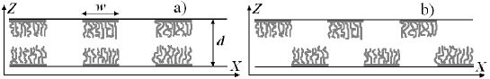
Figure 1: Geometry of the pore with in-phase (a) and out-of-phase (b) arrangement of the stripes with tethered polymer chains. The pore size is $d$ and the stripes width is $w$. The length of polymer chains is $L=20$ beads.

The method is extended to include the smooth repulsive walls via the reflection algorithm that preserves the total momentum [44]. The reduced number density for beads is equal to $\rho=3.0$. Polymer chains are built of $L=20$ beads linked via harmonic bonds. The grafting points have been fixed on each wall and are distributed randomly inside the stripes with a reduced grafting density $\rho_{\mathrm{g}}=1.0$. More details are provided elsewhere [44].

Two bead sorts, A and B, are considered. Polymer chains are made of beads of sort A. The total number of polymer beads in the system is $N^{\mathrm{p}}_{\mathrm{A}}$. A binary fluid mixture (which fills the interior of the pore) contains $N^{\mathrm{s}}_{\mathrm{A}}$ beads of sort A and $N_{\mathrm{B}}$ beads of sort B. The fraction of the beads of sort B is $f_{\mathrm{B}}=N_{\mathrm{B}}/N$, where $N=N^{\mathrm{p}}_{\mathrm{A}}+N^{\mathrm{s}}_{\mathrm{A}}+N_{\mathrm{B}}$ is the total number of the beads. Repulsion parameters for A–A and B–B pairs are defined to be the same, $a_{\mathrm{AA}}=a_{\mathrm{BB}}=25$, the choice being based on matching the compressibility of the model system (at $\rho=3.0$) to that of water, as discussed in [46]. Poor miscibility between A and B beads is set by the higher value of $a_{{\mathrm{AB}}}$ for the A–B interaction as compared to $a_{{\mathrm{AA}}}$. The choice of $a_{{\mathrm{AB}}}$ value is quite flexible and we use the value of $a_{{\mathrm{AB}}}=40$ which corresponds to the regime of moderate to strong segregation and ensures firm separation between species.

To visualize the morphologies, we employ the following density grid approach. Simulation box is split into the grid of cubic cells with the linear dimension of $0.75\div 2.0$, depending on the simulation box size. Local densities for polymer A beads, $\rho^{\mathrm{p}}_{\mathrm{A}}(x,y,z)$, solvent A beads, $\rho^{\mathrm{s}}_{\mathrm{A}}(x,y,z)$, and solvent B beads, $\rho_{\mathrm{B}}(x,y,z)$ are evaluated in each cell centered at $(x,y,z)$. They are averaged over $10-15$ configurations (the subsequent configurations are separated by $5000$ simulation steps). The averaging is carried out after the particular morphology is stabilized (typically, after $2\cdot 10^{5}$ simulation steps).

We found that presenting both local densities of A and B beads in the same snapshot is not very informative. Instead, we show separate snapshots for local density of A or of B beads. In the first case, we represent the cells with low local density of A beads $[\rho^{\mathrm{p}}_{\mathrm{A}}(x,y,z)+\rho^{\mathrm{s}}_{\mathrm{A}}(x,y,z)]/\rho<0.15$ as dots. All other cells are space-filled with the color saturation proportional to the value of $[\rho^{\mathrm{p}}_{\mathrm{A}}(x,y,z)+\rho^{\mathrm{s}}_{\mathrm{A}}(x,y,z)]/\rho$. The color tint is blueish if $\rho^{\mathrm{p}}_{\mathrm{A}}(x,y,z)>\rho^{\mathrm{s}}_{\mathrm{A}}(x,y,z)$ and greenish otherwise. Similar approach is used in the second case, when the density of B beads is plotted. In this case, $\rho_{\mathrm{B}}(x,y,z)$ is color coded with red tint.

3 Solvent-mediated transitions in special geometries

3.1 Wide stripes geometry

In the case of wide stripes that are in-phase arranged, the periodic pattern of alternating sub-regions is formed within the pore. The sub-regions free of polymer brush provide an environment for a bulk, quasi-3D demixing of confined A and B beads. On the contrary, the sub-regions dominated by a brush, reduce the volume accessible for the demixing of A and B beads to quasi-2D slabs, especially for moderate values of pore size $d$. This is demonstrated in figure 2, where we show examples of the morphologies observed for wide stripes with $w=90$ in a pore of size of $d=20$ when the fraction $f_{\mathrm{B}}$ is varied.

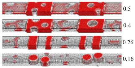
Figure 2: (Color online) The sequence of morphologies obtained for the case of wide stripes, $w=90$, at pore size $d=20$ by varying fraction of B beads, $f_{\mathrm{B}}$ (indicated on the right). Color-coded density of B beads in the selected part of the pore is shown only for the sake of clarity.

The first effect to mention is that with an increase of the fraction of A beads, $f_{\mathrm{A}}=1-f_{\mathrm{B}}$, more of them are adsorbed by the stripes of polymer brush causing their considerable swelling. We will discuss this effect quantitatively in section 4. The remaining A and B beads are spread within the rest of the accessible volume.

We will concentrate here on the phenomena that occur within quasi-3D sub-regions. The morphologies formed here repeat those observed for diblock copolymers at various composition (or in similar systems) [44, 45]. To relate both cases, one should look at the local fractions of A and B beads, $f^{\prime}_{\mathrm{A}}$ and $f^{\prime}_{\mathrm{B}}$, that differ from their global counterparts, $f_{\mathrm{A}}$ and $f_{\mathrm{B}}$, due to adsorption of some of A beads into the brush mentioned above. We found that cylinders made of B beads are formed at $f_{\mathrm{B}}=0.16$ ($f^{\prime}_{\mathrm{B}}=0.31$, lowest frame in figure 2). Similarly, cylinders made of A beads are observed inside the interval from $f_{\mathrm{B}}=0.40$ ($f^{\prime}_{\mathrm{A}}=0.26$) to $f_{\mathrm{B}}=0.50$ ($f^{\prime}_{\mathrm{A}}=0.17$), first and second frames from the top of figure 2. Lamellar-like phase (in the $OYZ$ plane; alternating blocks of A and B beads along the $X$-axis) is observed in the interval from $f_{\mathrm{B}}=0.26$ ($f^{\prime}_{\mathrm{A}}=0.50$) to $f_{\mathrm{B}}=0.30$ ($f^{\prime}_{\mathrm{A}}=0.42$), second frame from the bottom in figure 2. These boundaries of morphologies (in terms of the values $f^{\prime}_{U}$ for minor fraction $U$) correlate well with the phase diagram for diblock copolymers (see, e.g., [44, 45]).

Morphology transformations observed within the quasi-2D regions literally repeat those found for the narrow stripes geometry, and this case is considered in detail in the following subsection.

3.2 Narrow stripes geometry

For narrow stripes, $w<5$, the polymer chains from adjacent stripes bridge themselves into lamellae that envelope each wall [44]. It is quite obvious that the same scenario holds for the out-of-phase arrangement of stripes, as far as both surfaces are decoupled. This is confirmed in our simulations (not shown for the sake of brevity). Two flat lamellae, formed at each wall, reduce the region accessible to free A and B beads to a slab, which turns into a quasi-2D one for moderate pore size $d\sim 14\div 20$. This situation also represents the sub-regions dominated by a brush for the case of wide stripes (considered in the previous subsection).

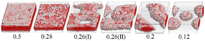
Figure 3: (Color online) Sequence of morphologies obtained for narrow stripes, $w=4$, in a pore of size $d=13.333$ at various fractions $f_{\mathrm{B}}$ (indicated at the bottom). From left to right: lamellar, thinned lamellar, perforated lamellar, ‘‘sausage’’ and ‘‘cake’’, single ‘‘sausage’’, and hexagonally packed ‘‘cakes’’ morphologies are shown (only color-coded density of B beads is shown).

In figure 3, we display the sequence of quasi-2D morphologies that appear in this central slab as the result of a micro-phase separation between A and B beads. The pore size is $d=13.333$, the stripes width is $w=4$ and only color-coded density of B beads is shown (in red tint). This pore size is a special one, as far as for the parameters being used here (polymer length, bulk and grafting densities), no solvent A beads are present at $f_{\mathrm{B}}=0.5$ [44]. At this fraction $f_{\mathrm{B}}$, solvent B beads fill-in all the slab-like accessible volume in the middle of the pore (first frame from the left in figure 3). The slab stays continuous but thins out with a decrease of $f_{\mathrm{B}}$ down to $f_{\mathrm{B}}=0.28$ (the next frame). Then, it turns into a perforated lamellar one and then into disjointed prolate and/or oblate objects made of beads B (see respective frames in figure 3). For still lower value of $f_{\mathrm{B}}$, $f_{\mathrm{B}}\approx 0.12$, there appear hexagonally distributed ‘‘cookies’’ of B beads. One can easily see that this morphology possesses the same symmetry as the perforated lamellar one, if beads A and B are interchanged. Further decrease of $f_{\mathrm{B}}$ causes the loss of hexagonal order of the ‘‘cookies’’, and for $f_{\mathrm{B}}<0.1$ the ‘‘cookies’’ of B beads become randomly arranged (not shown). This sequence of the morphologies is reminiscent of the one observed in partial mixing of the two-dimensional fluids [47]. Therefore, the case of narrow stripes can be classified as geometry-driven dimensional crossover from 3D to 2D for a confined fluid.

3.3 Pillar geometry

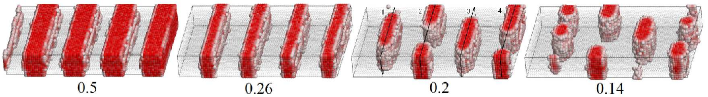
Figure 4: (Color online) Sequence of morphologies obtained for $d=13.333$ and $w=10$ at various fractions $f_{\mathrm{B}}$ (indicated at the bottom). Blocks of B beads filling the space between pillars of A beads ($f_{\mathrm{B}}=0.50$), thinned blocks ($f_{\mathrm{B}}=0.26$), hexagonally arranged columns ($f_{\mathrm{B}}=0.20$), and random columns ($f_{\mathrm{B}}=0.14$) are shown. Only color-coded density of B beads is displayed.

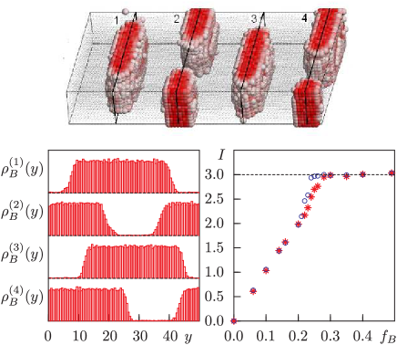
Figure 5: (Color online) Left bottom frame shows the density profiles $\rho^{(i)}(y)$ along each $i$-th slab region shown in the top frame. Right bottom frame shows the dependence of the integral profile $I$ (averaged over four slabs) on $f_{B}$. The results for simulation set I are shown as blue disks and for the set II — as red asterisks.

In the case of wider stripes ($w>6$), bridging of polymer chains that belong to adjacent stripes is prohibited due to high penalty in conformational entropy. Instead, the in-phase arranged stripes can bridge themselves across the pore to form pillars, providing that the pore width $d$ is not too big (cf. the sketch phase diagram presented in the previous work [44]). Such pillars are observed, for example, at $d=13.333$ and $w=10$. Similarly to the case shown in figure 2, the system again displays (periodic along $X$ axis) the pattern of sub-regions, one being pillars of merged brushes and another being polymer-free sub-regions. At $f_{\mathrm{B}}=0.5$, the latter are in a form of blocks filled exclusively with solvent B beads. For $0.5>f_{\mathrm{B}}>0.26$, these blocks become thinner first (as far as solvent A beads are adsorbed into pillars causing the latter to swell). Then, for $f_{\mathrm{B}}\sim 0.20$, the blocks split into rounded ‘‘columns’’ spanning across the pore and arranged almost hexagonally. At still lower values of $f_{\mathrm{B}}$, we arrive at randomly arranged columns of B beads of random thickness. All these morphologies are displayed in figure 4.

The regions accessible to the micro-phase separation of solvent beads have a shape of slabs extended along $Y$-axis. The important point here is that all morphologies observed within these slabs at various $f_{\mathrm{B}}$ are uniform within the $X$ dimension of each slab. Thus, the behavior of the system can be interpreted as being quasi-1D along $Y$ axis within each slab. One can quantify the observed morphology changes by the density profiles of B beads, $\rho(y)$, along $Y$ axis. It can be evaluated within a thin cross-section slabs located in the middle of each region (marked as $1-4$ in the top frame in figure 5). The thickness of each cross-section slab in $X$ direction is equal to $2$ and the averaging of the density is made in $Z$-direction. The histograms for the density profiles $\rho^{(i)}(y)$ in each $i$-th slab obtained in this way for the morphology shown in the top frame in figure 5, are presented in the left bottom frame of figure 5. The local density inside each column of B beads is equal to the bulk density, $\rho(y)\approx\rho=3$, whereas it drops down to zero outside the column. Therefore, the integrated density, $I=\int_{0}^{L_{y}}\mathrm{d}y\rho(y)/L_{y}$ is a good measure for ‘‘block continuity’’. Right hand frame in figure 5 shows the values of $I$ averaged over all four slabs, $1-4$. Two sets of simulations were performed. For the set I we started the simulation from the morphology equilibrated at $f_{\mathrm{B}}=0.5$ and converted the required number of B beads, chosen randomly across the system, into A beads. In the set II simulation, the initial configuration involved linearly stretched polymer chains and solvent A and B beads randomly distributed within the pore.

One can observe the transformation from continuous into discontinuous block morphology that occurs at $f^{*}_{\mathrm{B}}\approx 0.23$ (for the simulations set I; blue open disks) or at $f^{*}_{\mathrm{B}}\approx 0.28$ (for the simulation set II; red asterisks). The former value is lower which indicates the presence of the ‘‘underconcentrated’’ continuous block morphology at $0.28>f_{\mathrm{B}}>0.23$ in the simulations set I. It is also interesting to note that for small $f_{\mathrm{B}}$, the integral $I$ changes nearly linearly with $f_{\mathrm{B}}$.

4 Competition between solvent mediated morphologies for closely
arranged stripes

So far we considered several special cases when both the geometry restrictions imposed by the pore geometry and the composition of the mixture confined within the accessible sub-regions promote essential morphological changes. In both cases of a narrow pore (subsection 3.2) and of a pillar (subsection 3.3), the stripes of brushes are bridged in one of the directions by purely geometrical means, literally by bringing stripes close enough to form lamellae (pillars). The role of the solvent is restricted to the swelling of the already formed lamellae (pillars) and to a micro-phase separation inside the polymer-free sub-regions.

However, one can envisage the situation when the lamellar (pillar) bridges are formed exclusively due to the action of a solvent. Apparently, this is possible in the geometries where the stripes of brush are brought sufficiently close in one of $X$ or $Z$ dimensions, but not close enough to bridge over by themselves. Even a more promising case can be designed by provoking the competition between the bridging, which may happen when the stripes are positioned sufficiently close in both $X$ and $Z$ directions. Possible technological applications could involve the use of a solvent mixture which contains A component in the form of a short chain. This component could be first used for demixing with the B component and for the formation of certain morphology, and then to be used as a crosslinker to permanently fix the structure.

4.1 Mechanism for solvent-mediated morphologies and quantitative characterization of brush bridging and deformation of chains

The mechanism for the solvent-mediated morphologies lies in the swelling of a polymer brush due to adsorption of a good solvent, the effect already mentioned above. Here, we will discuss this effect in more detail. Let us consider the environment within the stripes of polymer chains. Due to relatively low grafting density $\rho_{\mathrm{g}}=\frac{1}{3}\rho$ (where $\rho=3$ is bulk number density), the stripes are far from the regime of a dense brush [48] and are exposed to the available solvent. For the case of poor solvent, the brush collapses and each chain is in a regime of polymer melt, whereas for a good solvent, the chains are expected to be in the regime of a good solution. Two cases are well distinguished by their respective scaling laws [49]. For instance, the radius of gyration scales as:

$$R_{\mathrm{g}}=R\left[l_{0}(N-1)\right]^{\nu}\,,$$ (1)

where $R=\mathrm{const}$, $l_{0}$ is the equilibrium bond length, $N$ is the number of monomers and $\nu=0.5$ for the case of polymer melt and $\nu\approx 0.59$ (Flory exponent) for the case of a good solution [49]. As it was discussed previously [50], the softness of the potentials employed in typical DPD simulations does not violate the correct value for the exponent $\nu=0.59$ for a single chain in a good solvent.

To check whether this scenario holds, we performed a set of simulations for the pore geometry with well separated stripes. Polymer chains are made of A beads and a one-component solvent of C beads is used. The quality of the solvent is tuned via the repulsion parameter $a_{{\mathrm{AC}}}$ between A and C beads ranging from $25$ (good solvent) up to $40$ (bad solvent). For each simulation run, the average bond length $l_{0}$ and the radius of gyration $R_{\mathrm{g}}$ were evaluated and the scaling law (1) was employed for the assumed values of the exponent $\nu$, $\nu=0.5$ or $0.59$. Next, the prefactor $R$ (see equation (1) was estimated. The results are collected in table 1. As it follows from the enclosed data, the difference between the estimated prefactors $R$ does not exceed 1% which proves that the scaling law (1) holds consistently. These simulations confirm a crossover from the regime of polymer melt to a good solution regime for each chain which is driven by the quality of the solvent. Typical chain extension ratio is estimated as $[l_{0}(N-1)]^{0.09}\sim 1.3$ which is of the order of $2\div 4$ unit lengths for our particular model, and this provides the length scale for brush separations at which one expects solvent-mediated bridging.

Table 1: Results of fitting the average bond length $l_{0}$ and radius of gyration $R_{\mathrm{g}}$ to the scaling law, equation 1, for the assumed values of the exponent $\nu$. Output: prefactor $R$ in equation 1 is numerically consistent for all the cases considered.

pore geometry	solvent	$l_{0}$	$R_{g}$	$R$
$d=22$, in-phase	$a_{{\mathrm{AC}}}=40$ $(\nu=0.50)$	0.893	1.909	0.463
	$a_{\mathrm{AC}}=25$ $(\nu=0.59)$	0.937	2.557	0.468
$d=20$, out-of-phase	$a_{\mathrm{AC}}=40$ $(\nu=0.50)$	0.892	1.909	0.464
	$a_{\mathrm{AC}}=25$ $(\nu=0.59)$	0.936	2.558	0.468

To quantitatively characterize the level of bridging between stripes we introduce the overlap integrals $I_{x}$ and $I_{z}$ between polymer chains in $X$ and $Z$ directions (by analogy to the case of uniform brushes [51]):

$$I_{x}=\sum_{\langle ik\rangle}\int_{0}^{L_{x}}\rho_{i}(x)\rho_{k}(x)\mathrm{d}x\cdot\left[\sum_{\langle ik\rangle}\int_{0}^{L_{x}}\mathrm{d}x\right]^{-1}\qquad I_{z}=\int_{0}^{d}\rho_{\mathrm{bot}}(z)\rho_{\mathrm{top}}(z)\mathrm{d}z\cdot\left[\int_{0}^{d}\mathrm{d}z\right]^{-1}\!\!\!\!\!\!\!\!,$$ (2)

where $\rho_{i}(x)$ is the density profile along $X$ axis for polymer beads belonging to $i$-th stripe (averaged over $Y$ and $Z$ directions); $\rho_{\mathrm{bot}}(z)$ and $\rho_{\mathrm{top}}(z)$ are density profiles for polymer beads belonging to the bottom or top wall, respectively (averaged over $X$ and $Y$ directions). These density profiles are illustrated in figure 6. The evaluation of $I_{x}$ overlap integral is performed over all $\langle ik\rangle$ pairs that are located at the same wall and are adjacent in $X$ direction (with the account of the periodic boundary conditions).

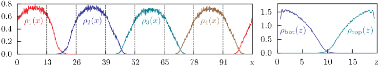
Figure 6: (Color online) Left hand frame illustrates the density distributions $\rho_{i}(x)$ of the polymer beads in each $i$-th stripe along $X$ axis averaged over $Y$ and $Z$ axes (the distributions $1-4$ belonging to the bottom surface are shown only). Right hand frame illustrates the density distributions of the polymer beads along $Z$ axis that belong to bottom and top surfaces (abbreviated as ‘‘bot’’ and ‘‘top’’, respectively), the distributions are averaged in $X$ and $Y$ directions.

The bridging of brushes involves a certain amount of bending and/or anisotropic stretching of polymer chains. These can be quantified via the components of gyration tensor, $G_{xx}$, $G_{yy}$ and $G_{zz}$. The components are evaluated for each $k$-th chain

$$G_{\alpha\beta}^{[k]}=\frac{1}{N}\sum_{i=1}^{N}\left(r_{i,\alpha}^{[k]}-R_{\alpha}^{[k]}\right)\left(r_{i,\beta}^{[k]}-R_{\beta}^{[k]}\right),$$ (3)

where $\alpha,\beta$ denote Cartesian axes, $r_{i,\beta}^{[k]}$ are the positions of individual monomers and ${R}^{[k]}$ is the center of mass position of the $k$-th chain. Then, $G_{\alpha\beta}^{[k]}$ are averaged over the chains and over the time trajectory after the morphology stabilizes itself, providing the estimates for $G_{xx}$, $G_{yy}$ and $G_{zz}$. One should mention that due to the symmetry of the pore in $Y$ direction, the $G_{yy}$ component is found to be unchanged and it is not considered in our analysis. The average radius of gyration $R_{\mathrm{g}}$ is defined as $R_{\mathrm{g}}^{2}=G_{xx}+G_{yy}+G_{zz}$, and the average extension of chains can be found from the maximal eigenvalue of the gyration tensor, $\sigma_{\max}^{2}$.

4.2 Solvent-mediated morphological changes

The properties introduced above are used to characterize solvent-mediated bridging between stripes of brushes. At first we will consider the case of one-component solvent of variable quality (tuned via $a_{\mathrm{AC}}$ parameter, see above). The results are provided for the pore size of $d=20$ and stripes of width $w=13$ arranged out-of-phase (see figure 7). With a decrease of $a_{\mathrm{AC}}$ towards the case of a good solvent ($a_{\mathrm{AC}}=25$), one observes a monotonous increase of all the metric properties, $G_{xx}$, $G_{zz}$ and $\sigma_{\max}^{2}$. This quantifies the effect of polymer chains swelling due to the crossover from the polymer melt to polymer in a good solvent regime. The overlap integrals $I_{x}$ and $I_{z}$ have been found to become non-zero at a certain threshold value of $a_{\mathrm{AC}}<28$. This indicates a solvent-mediated bridging between the droplets of polymer chains. The bridging happens almost simultaneously in both $X$ and $Z$ directions for this geometry of the pore. In view of our analysis, it is important to mention that all the characteristics, $I_{x}$, $I_{z}$, $G_{xx}$, $G_{zz}$ and $\sigma_{\max}^{2}$ increase monotonously with a decrease of $a_{\mathrm{AC}}$ down to $25$ with no peculiarities observed either in the behavior of metric properties and overlap integrals or in the snapshots.

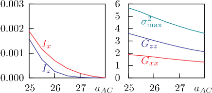
Figure 7: (Color online) Behavior of the overlap integrals $I_{x}$ and $I_{z}$ (left hand frame) and the components $G_{xx}$ and $G_{zz}$ and maximal eigenvalue $\sigma_{\max}^{2}$ of the gyration tensor (right hand frame) upon the changes of the quality of the one-component solvent. The quality of the solvent is defined via the repulsion parameter $a_{\mathrm{AC}}$ between polymer (A) and solvent (C) beads, the value of $a_{\mathrm{AC}}=25$ represents the case of a good solvent.

The case of a one-component solvent of the variable quality provides a suitable reference point for a more complex case of a two-component solvent composed of A and B beads. The repulsion parameter $a_{\mathrm{AB}}$ is chosen to be always equal to $40$ in our study. Therefore, the effective ‘‘goodness’’ of such a mixture can be characterized by the fraction $f_{\mathrm{B}}$ of B beads (the mixture is a good solvent for $f_{\mathrm{B}}=0$). The analogy with a one-component solvent is, however, not exact, as far as the mixture is prone to segregation (see, e.g. figure 4 in [44]). Local inhomogeneities may effect the way in which the brushes are bridged and, as a result, the sequence of solvent-mediated morphologies may differ from the case of a one-component solvent. Hereafter, we will consider the fixed stripe width of $w=13$ and both: in- and out-of phase arrangements. The pore size will be fine-tuned in each case and ranges from $d=19$ to $d=24$.

In the case of in-phase arrangement of the stripes, we select three pore sizes, namely $d=20,22$ and $24$ (the distance between brushes in $X$ and $Z$ directions is approximately the same for $d=22$). The evolution of $I_{x}$, $I_{z}$, $G_{xx}$, $G_{zz}$ and $\sigma_{\max}^{2}$ upon the change of the fraction of $f_{\mathrm{B}}$ from 0.5 down to 0 is shown for each pore size in figure 8. One can compare these plots with the curves displayed in figure 7 and observe that the metric properties of chains at $f=0.5$ subject to the two-component solvent, match approximately their counterparts for the case of a one-component solvent at $a_{\mathrm{AC}}=28$. This provides the estimate for an effective ‘‘goodness’’ of the two-component solvent. Metric properties coincide for the case of good solvent ($f=0$ and $a_{\mathrm{AC}}=25$, respectively).

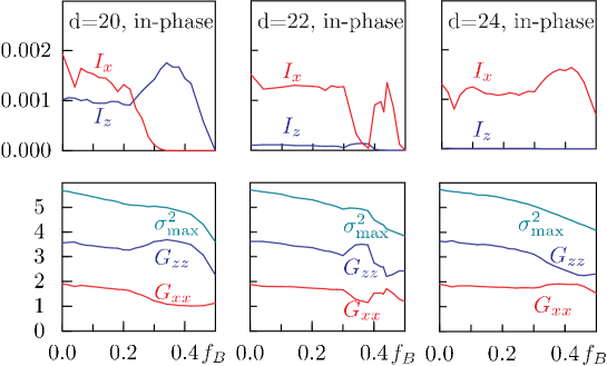
Figure 8: (Color online) Behavior of the overlap integrals $I_{x}$ and $I_{z}$ (top row of frames) and the components $G_{xx}$ and $G_{zz}$ and the maximal eigenvalue $\sigma_{\max}^{2}$ of the gyration tensor (bottom row of frames) upon the changes of the effective quality of the two-component solvent of A and B beads. Effective quality of the solvent is defined via the fraction $f_{\mathrm{B}}$ of ‘‘bad solvent’’ beads B. The case of in-phase arrangement of stripes of the width $w=13$ is shown at the pore sizes $d=20,22$ and $24$.

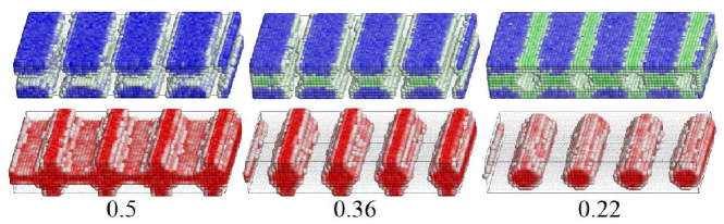
Figure 9: (Color online) Sequence of morphologies obtained for $d=20$ and for in-phase arranged stripes of the width $w=13$ at various fractions $f_{\mathrm{B}}$ (indicated at the bottom). Top row: color-coded densities of brush prevailing (blue) and good solvent prevailing (green) regions, bottom row: bad solvent prevailing regions (red). Morphologies: separate droplets ($f_{\mathrm{B}}=0.50$); solvent mediated pillars ($f_{\mathrm{B}}=0.36$) and in-lined cylinders of B beads ($f_{\mathrm{B}}=0.22$).

When one moves away from $f_{\mathrm{B}}=0.5$ towards $0$, the behavior of all the properties $I_{x}$, $I_{z}$, $G_{xx}$, $G_{zz}$ and $\sigma_{\max}^{2}$ differs much from the case of a one-component solvent. For the pore of $d=20$, the bridging in $Z$ direction is observed first. This is indicated by a large hill at $I_{z}$ centered around the value of $f_{\mathrm{B}}=0.34$ (top left hand frame in figure 8). To be able to form the pillar morphology, the chains need to rearrange themselves preferentially in $Z$ direction as indicated by an increase of $G_{zz}$ at the expense of $G_{xx}$ values (bottom left hand frame in figure 8). The value of $G_{zz}=3.69$ found at $f_{\mathrm{B}}=0.34$ is of the same order and even exceeds that observed at $f_{\mathrm{B}}=0$, namely $G_{zz}=3.56$. This indicates that the chains within pillars are in the regime of a good solvent. This is confirmed by the snapshots shown in top-middle and bottom-middle columns of figure 9, where the droplets merge together by the good solvent beads. Therefore, as a result of a different miscibility of A and B components, the solvent A nucleates by filling the gap between polymer droplets, and the solvent mediated transition from separate droplets to pillar morphology occurs. With a further decrease of $f_{\mathrm{B}}$, the pillars are also bridged in $X$ direction. This is indicated by an increase of $G_{xx}$ values and is seen in the top-right and bottom-right columns of figure 9.

With an increase of the pore size $d$ to $22$, the bridging capability in $Z$ direction is lessened giving a way for bridging along the walls. This is demonstrated by the existence of local maxima and minima of $I_{x}$, $I_{z}$ and $G_{xx}$ and $G_{zz}$ components (see top-center and bottom-center frames in figure 8). With a further increase of $d$ to $24$, the situation is reversed with respect to the case of $d=20$. Now, the droplets are farther in $Z$ direction and their bridging is observed in $X$ direction: $I_{x}$ and $G_{xx}$ possess maxima centered around $f_{\mathrm{B}}=0.4$ (top-right and bottom-right frames of figure 8).

Let us switch now to the case of out-of-phase arrangement of stripes. The set of pore sizes $d=19,20$ and $d=21$ are analyzed in this case (the distance between brushes in $X$ and $Z$ directions is approximately the same for $d=20$). The behavior of $I_{x}$, $I_{z}$, $G_{xx}$, $G_{zz}$ and $\sigma_{\max}^{2}$ is shown in figure 10. The limiting cases of $d=19$ and $d=21$ bear similarities to their respective counterparts ($d=20$ and $d=24$) for the in-phase arrangement of stripes. Indeed, at $d=19$, the polymer-rich droplets are bridged in $Z$ direction first with a decrease of $f_{\mathrm{B}}$. With a further decrease of $f_{\mathrm{B}}$, the droplets are bridged in $X$ direction. Situation is reversed at $d=21$.

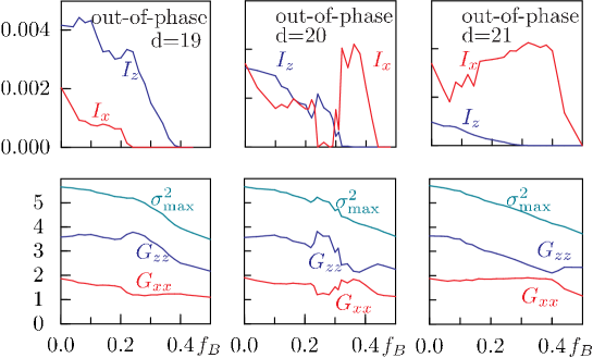
Figure 10: (Color online) The same properties as in figure 8 are shown for the case of out-of-phase arrangement of stripes of the width $w=13$ at the pore sizes $d=19,20$ and $21$.

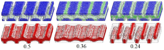
Figure 11: (Color online) Sequence of morphologies obtained for $d=20$, for out-of-phase arranged stripes of the width of $w=13$ at various fractions of $f_{\mathrm{B}}$. Separate droplets ($f_{\mathrm{B}}=0.50$); modulated lamellar ($f_{\mathrm{B}}=0.36$) and meander ($f_{\mathrm{B}}=0.24$) morphologies.

The intermediate case of the pore size $d=20$ is more interesting because it demonstrates a solvent mediated switching between various morphologies. When $f_{\mathrm{B}}$ decreases away from 0.5, first the bridges in $X$ direction are formed. Both $I_{x}$ and $G_{xx}$ exhibit maxima centered around $f_{\mathrm{B}}=0.36$, cf. top-middle and bottom-middle frames of figure 10. This indicates the formation of a solvent mediated lamellar morphology, see snapshots in top-middle and bottom-middle frames of figure 11. With a further decrease of $f_{\mathrm{B}}$, the bridges are formed in $Z$ direction at the expense of those that have been previously formed in $X$ direction. This is indicated by a large value of $I_{z}$ and by practically zero value of $I_{x}$ within the interval of $f_{\mathrm{B}}\in[0.23,0.3]$. The structure of this morphology is of simple meander (see snapshots in top-right and bottom-right hand frames of figure 11).

One can see that when the fraction of good solvent in a system increases, the chains within each stripe swell and acquire certain bistability properties. The chains can redistribute their mass either in $X$ or in $Z$ direction (as indicated by the behavior of $G_{xx}$ and $G_{zz}$ components) and form the bridges (as indicated by non-zero values of the overlap integrals $I_{x}$ and $I_{z}$). The histograms for the corresponding components of the gyration tensor, $f(G_{xx})$ and $f(G_{zz})$ provide additional insight into spatial redistribution of the polymer chains in various morphologies. These histograms are shown in figure 12 for the case of pore size $d=20$ and out-of-phase arrangement of the stripes of the width of $w=13$. The distribution function $f(G_{zz})$ is found to be essentially stretched towards larger values of $G_{zz}$ for meander ($f_{\mathrm{B}}=0.26$) morphology and at still lower values of $f_{\mathrm{B}}$. It exhibits a quite irregular shape, whereas the distribution of $f(G_{xx})$ is similar to the Lhuillier form [52, 53, 50] that was found as a typical distribution of experimental radii of gyration for long polymers. Broad distributions of a gyration tensor of both components indicate the existence of weakly and highly deformed chains within each stripe. It is plausible to assume that highly deformed chains are found within the bridges that connect polymer droplets in a solvent mediated pillar, meander and possibly other morphologies. A measure for the average stretch of chains is provided by the maximal eigenvalue of the gyration tensor, $\sigma_{\max}^{2}$. As it follows from the set of plots shown in figures 8 and 10, the values of $\sigma_{\max}^{2}$ exhibit local maxima for certain morphologies. The values of these maxima are higher compared to the case of one-component solvent mapped into an effective value of $a_{\mathrm{AC}}$ (see figure 7). This indicates that the loss of conformation entropy due to an excessive average stretch of chains is compensated by a decrease of the enthalpy caused by an increase of contacts between similar beads of type A.

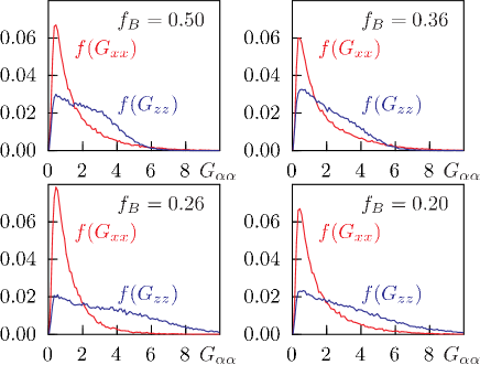
Figure 12: (Color online) Distributions of the relevant gyration tensor components, $G_{xx}$ and $G_{zz}$ for various fractions $f_{\mathrm{B}}$ (indicated in each frame). The case of $d=20$, $w=13$ and out-of-phase arrangement of stripes is shown.

5 Summary

In this work we consider the formation and transitions between the nanostructures that occur inside a pore modified by stripes of tethered polymer brushes filled with a binary mixture. The beads A of filler solvent are identical to those of chain monomers, while the beads B exhibit a partial mixing with beads A. Compared to our previous study [44], a number of extensions are made. In particular, two options of in- and out-of-phase arrangement of polymer stripes are considered. Apart from that, we examine in detail the effect that the composition of A and B beads produces on the formation of the morphologies in a broad range of pore geometries. At last, for some characteristic cases we undertook supplementary simulations with the one-component solvent of variable quality which replaces the mixture to serve as a reference.

The change of the composition of the fluid inside the pores has a great impact on the developing structures. For pore geometries with narrow stripes, the problem of the description of microphase separation inside the pore reduces to quasi two-dimensional; in the case of moderately wide stripes and narrow pore, one faces quasi one-dimensional demixing; whereas for very wide stripes, the system is split into quasi two-dimensional and bulk regions.

The most interesting effects, in our view, that demonstrate solvent mediated changes in the nanostructures occur for the geometries with weakly separated stripes of polymer chains. With an increase of A component, the latter dissolves the polymer chains and causes their swelling. As a result, the system acquires a bistability in terms of either bridging the adjacent stripes along the wall or bridging the opposite stripes across the pore. Stable morphology is formed due to competition between segregation of A and B beads and the deformation of the chains. In our simulations we observe morphology switching due to subtle changes in pore geometry and/or in the composition of a mixture.

We found the following solvent mediated morphologies: in-lined cylinders (made of one component), meander structure and wave-shaped modulated internal channels. The suggested applications of such structures (possibly, after making the structure permanent via crosslinking) involve nanopatterning for manufacturing of nanochannels, nanorods and similarly sized objects.

So far our studies concentrated on the equilibrium DPD simulations. However, it would be of interest to check how the morphologies change if the fluid undergoes a pressure-driven flow along the pore axis. This problem is currently under study in our laboratories.

Ukrainian 0

Фазовi переходи за посередництва розчинника у порах
iз стiнками декорованими полiмерними щiтками. Комп’ютерне моделювання методом
дисипативної динамiки Я.М. Iльницький${}^{\textsf{\footnotesize{\mbox{?}}}}$, С.Соколовскi${}^{\textsf{\footnotesize{\mbox{?}}}}$, Т. Пацаган${}^{\textsf{\footnotesize{\mbox{?}}}}$

             
${}^{\textsf{\footnotesize 1}}$ Iнститут фiзики конденсованих систем НАН України, вул. I. Свєнцiцького, 1, 79011 Львiв, Україна ${}^{\textsf{\footnotesize 2}}$ Вiддiл моделювання фiзико-хiиiчних процесiв, Унiверситет Марiї Кюрi-Склодовської,
20031 Люблiн, Польща

References

- [1] De Gennes P.G., Rev. Mod. Phys., 1985, 57, 827; doi:10.1103/RevModPhys.57.827.
- [2] Advincula R.C., Brittain W.J., Caster K.C., Ruhe J., Polymer Brushes: Synthesis, Characterization, Applications, Willey, New York, 2004.
- [3] Rühe J., Ballauf M., Biesalski M., Dziezok P., Grohn F., Johannsmann D., Houbenov N., Hugenberg N., Konradi R., Minko S., Motornov M., Netz R.R., Schmidt M., Seidel C., Stamm M., Stephan T., Usov D., Zhang H.N., Adv. Polym. Sci., 2004, 165, 79; doi:10.1007/b11268.
- [4] Naji A., Seidel C., Netz R.R., Adv. Polym. Sci., 2006, 198, 149; doi:10.1007/12_062.
- [5] Klushin L.I., Skvortsov A.M., J. Phys. A: Math. Theor., 2011, 44, 473001; doi:10.1088/1751-8113/44/47/473001.
- [6] Binder K., Kreerb T., Milchev A., Soft Matter, 2011, 7, 7159; doi:10.1039/c1sm05212h.
- [7] Polymer Brushes, Advincula R.C., Brittain W.J., Caster K.C., Rühe J. (Eds.), Wiley-VCH, Weinheim, 2004.
- [8] Descas R., Sommer J.-U., Blumen A., Macromol. Theory Simul., 2008, 17, 429; doi:10.1002/mats.200800046.
- [9] Garbassi F., Morra M., Occhiello E., Polymer Surfaces: From Physics to Technology, John Wiley & Sons; New York, 2002.
- [10] Sperling L.H., Polymeric Multicomponent Materials: An Introduction LED, Wiley Interscience, New York, 1997.
- [11] Klein J., Science, 2009, 323, 47; doi:10.1126/science.1166753.
- [12] Napper D.H., Polymeric Stabilization of Colloidal Dispersions, Academic, London, 1983.
-
[13]
Storm G., Belliot S.O., Daemen T., Lasic D.D., Adv. Drug
Delivery Rev., 1995, 17, 31;
doi:10.1016/0169-409X(95)00039-A. - [14] Hucknall A., Rangarajan S., Chilkoti A., Adv. Mater., 2009, 21, 2441; doi:10.1002/adma.200900383.
- [15] Wang A.J., Xu J.J., Chen H.Y., J. Chromatogr. A, 2007, 1147, 120; doi:10.1016/j.chroma.2007.02.030.
-
[16]
Li Y., Zhang J., Fang L., Wang T., Zhu S., Li Y., Wang Z., Zhang L.,
Cui L., Yang B., Small, 2011, 7, 2769;
doi:10.1002/smll.201100313. - [17] Guskova O.A., Seidel C., Macromolecules, 2011, 44, 671; doi:10.1021/ma102349k.
- [18] Wang J., Müller M., Macromolecules, 2009, 42 , 2251; doi:10.1021/ma8026047.
- [19] Yin Y., Sun P., Li B., Chen T., Jin Q., Ding D., Shi A.-C., Macromolecules, 2007, 40, 5161; doi:10.1021/ma070393n.
- [20] Bormashenko E., Pogreb R., Stanevsky O., Bormashenko Y., Tamir S., Cohen R., Nunberg M., Gaisin V.Z., Gorelik M., Gendelman O.V., Mater. Lett., 2005, 59, 2461; doi:10.1016/j.matlet.2005.03.015.
- [21] Nagpal U., Kang H., Craig G.S.W., Nealey P.F., de Pablo J.J., ACS Nano, 2011, 5, 5673; doi:10.1021/nn201335v.
- [22] Cao Q., Zuo C., Li L., Yang Y., Li N., Microfluid Nanofluid, 2011, 10, 977; doi:10.1007/s10404-010-0726-9.
- [23] Chen T., Amin I., Jordan R., Chem. Soc. Rev., 2012, 41, 3280; doi:10.1039/c2cs15225h.
-
[24]
Guangsuo L., Fabrication of nanopatterns via surface chemical modification and
reactive reversal nanoimprint lithography, PhD Thesis, National University of Singapore,
Singapore, 2010,
http://scholarbank.nus.edu.sg/handle/10635/22850. - [25] Tolfree D.W.L., Rep. Prog. Phys., 1998, 61, 313; doi:10.1088/0034-4885/61/4/001.
- [26] Burmeister F., Schläfle C., Keilhofer B., Bechinger C., Boneberg J., Leiderer P., Adv. Mater., 1998, 10, 495; doi:10.1002/(SICI)1521-4095(199804)10:6<495::AID-ADMA495>3.0.CO;2-A.
-
[27]
Knight J.B., Vishwanath A., Brody J.P., Austin R.H., Phys. Rev. Lett., 1998, 80, 3863;
doi:10.1103/PhysRevLett.80.3863. - [28] Surface-Initiated Polymerization I and II, Jordan R. (Ed.), Adv. Polym. Sci., 197-198, 2006.
- [29] Zhou X., Chen Y., Li B., Lu G., Boey F.Y.C., Ma J., Zhang H., Small, 2008, 4, 1324; doi:10.1002/smll.200701267.
- [30] Schmelmer U., Paul A., Küller A., Steenackers M., Ulman A., Grunze M., Gölzhäuser A., Jordan R., Small, 2007, 3, 459; doi:10.1002/smll.200600528.
- [31] Adamczyk P., Romiszowski P., Sikorski A., Catal. Lett., 2009, 129, 130; doi:10.1007/s10562-008-9795-8.
-
[32]
Chang C.-Y., Yang H.-W., Lin J.-S., Ju S.-P., Hsieh J.-Y., J. Comput. Theor. Nanosci., 2011, 8,2439;
doi:10.1166/jctn.2011.1976. - [33] Singh S.K., Khan S., Jana S., Singh J.K., Mol. Simulat., 2011, 37, 350; doi:10.1080/08927022.2010.514778.
- [34] Koutsioubas A.G., Vanakaras A.G., Langmuir, 2008, 24, 13717; doi:10.1021/la802536v.
- [35] Chen H., Chen X., Ye Z., Liu H., Hu Y., Langmuir, 2010, 26, 6663; doi:10.1021/la904001h.
- [36] Jayaraman A., Hall C.K., Genzer J., J. Chem. Phys., 2005, 123, 124702; doi:10.1063/1.2043048.
- [37] Chen H., Peng C., Sun L., Liu H., Hu Y., Jiang J., Langmuir, 2007, 23, 11112; doi:10.1021/la701773a.
-
[38]
Spaeth J.R., Dale T., Kevrekidis I.G.,
Panagiotopoulos A.Z., Ind. Eng. Chem. Res., 2011, 50, 69;
doi:10.1021/ie100337r. - [39] Patra M., Linse P., Nano Lett., 2006, 6, 133; doi:10.1021/nl051611y.
- [40] Goujon F., Malfreyt P., Tildesley D.J., J. Chem. Phys., 2008, 129, 034902; doi:10.1063/1.2954022.
- [41] Li C.-S., Wu W.-C., Sheng Y.-J., Chen W.-C., J. Chem. Phys., 2008, 128, 154908; doi:10.1063/1.2904866.
- [42] Petrus P., Lísal M., Brennan J.K., Langmuir, 2010, 26 3695; doi:10.1021/la903200j.
- [43] Petrus P., Lísal M., Brennan J.K., Langmuir, 2010, 26, 14680; doi:10.1021/la102666g.
- [44] Ilnytskyi J.M., Patsahan T., Sokołowski S., J. Chem. Phys., 2011, 134, 204903; doi:10.1063/1.3592562.
-
[45]
Ilnytskyi J.M., Patsahan T., Holovko M., Krouskop P.E.,
Makowski M.P., Macromolecules, 2008, 41, 9904;
doi:10.1021/ma801045z. - [46] Groot R.D., Warren P.B., J. Chem. Phys., 1997, 107, 4423; doi:10.1063/1.474784.
- [47] Zhao Y., Liu H., Lu Zh., Sun Ch., Chin. J. Chem. Phys., 2008, 21, 451; doi:10.1088/1674-0068/21/05/451-456.
- [48] Romeis D., Merlitz H., Sommer J.U., J. Chem. Phys., 2012, 136, 044903; doi:10.1063/1.3676657.
- [49] De Gennes P.G., Scaling Concepts in Polymer Physics, Cornell University Press, Ithaca and London, 1979.
- [50] Ilnytskyi J.M., Holovatch Yu., Condens. Matter Phys., 2007, 10, 539; doi:10.5488/CMP.10.4.539.
- [51] Kreer T., Müser M.H., Binder K., Klein J., Langmuir, 2001, 17, 7804; doi:10.1021/la010807k.
- [52] Lhuillier D., J. Phys., 1988, 49, 705; doi:10.1051/jphys:01988004905070500.
- [53] Victor J.M., Lhuillier D., J. Chem. Phys., 1990, 92, 1362; doi:10.1063/1.458147.
Ukrainian \adddialect\l@ukrainian0 \l@ukrainian