Scale-dependent bias from multiple-field inflation

Abstract

We provide a formula for the scaling behaviour of the inflationary bispectrum in the ‘squeezed’ limit where one momentum becomes much smaller than the other two. This determines the scaling of the halo bias at low wavenumber and will be an important observable for the next generation of galaxy surveys. Our formula allows it to be predicted for the first time for a generic inflationary model with multiple light, canonically-normalized scalar fields.

For the last twenty years, our information about the very early universe has primarily come from the large-scale anisotropies of the cosmic microwave background (CMB). But over the next decade fresh data will come from a new generation of large-scale structure surveys such as Euclid and LSST, and complementary small-scale CMB observations such as PIXIE [1, *Ivezic:2008fe, *Kogut:2011xw].

These surveys will probe a new suite of observables, requiring the development of techniques by which they can be predicted from models of the early universe. In this Letter we focus on an observable which will be a target for future surveys—the scale-dependent halo bias, which is sensitive to the scaling of the primordial bispectrum in the so-called squeezed limit. It is a discriminant of inflationary models with more than one active field [4, *Sefusatti:2009xu, *Giannantonio:2011ya, *Becker:2012yr, *Becker:2012je, 9].

Scale-dependent bias.—We cannot observe the primordial density field itself, but only correlations between populations of objects which trace its properties. One such population are halos of mass $M$, which form from collapse of over-dense regions. The clustering of these halos is described by the halo–halo or matter–halo power spectra $P^{\mathrm{h}\mathrm{h}}$ and $P^{\delta\mathrm{h}}$, where $\delta$ is the primordial density contrast. At lowest order the relationship between $\delta$ and the halo number density is linear $P^{\delta\mathrm{h}}(k)\approx b_{\mathrm{L}}P^{\delta\delta}_{R}(k)$ and therefore $P^{\mathrm{h}\mathrm{h}}(k)\approx b_{\mathrm{L}}^{2}P^{\delta\delta}_{R}(k)$. The superscript ‘$R$’ denotes smoothing over a lengthscale $R$ sufficiently large to enclose the halo mass $M$.

Corrections to $b_{\mathrm{L}}$ come from higher-order correlations of $\delta$. They can be expressed using the $n$-point functions of the curvature perturbation $\zeta$, which is typically used to characterize predictions of inflationary models. The leading effect comes from the three-point function and induces a $k$-dependent shift $b_{\mathrm{L}}\rightarrow b_{\mathrm{L}}+\delta b(k)$, where [10, *Dalal:2007cu, *Slosar:2008hx, 13]

$$\begin{split}\delta b(k)=\frac{M_{R}^{-1}(k,z)}{4\pi^{2}\sigma^{2}_{M}}&\Big{(}\frac{\delta_{\mathrm{c}}^{2}}{\sigma^{2}_{M}}-1\Big{)}\int_{0}^{\infty}q^{2}\mathrm{d}q\;M_{R}(q,z)\\ &\mbox{}\times\int_{-1}^{1}\mathrm{d}\mu\;M_{R}(Q,z)\frac{B_{\zeta}(k,q,Q)}{P_{\zeta}(k)}.\end{split}$$ (1)

Here, $z$ is the redshift and $Q^{2}\equiv k^{2}+q^{2}+2\mu kq$; the critical density for spherical collapse is $\delta_{\mathrm{c}}\simeq 1.69$; and $\sigma^{2}_{M}$ is the variance of the tracing population of mass-$M$ halos . The kernel $M_{R}(q,z)$ is related to the linearized Poisson equation connecting the density contrast $\delta(\bm{\mathrm{{k}}},z)$ and $\zeta(\bm{\mathrm{{k}}})$. It can be written as

$$M(k,z)=\frac{2}{5}\frac{k^{2}}{H_{0}^{2}}\frac{T(k)}{\Omega_{\mathrm{m},0}}\frac{g(z)}{1+z}.$$ (2)

The transfer function $T(k)$ is normalized to unity as $k\rightarrow 0$, and $g(z)$ accounts for suppression of growth during $\Lambda$-domination. The present-day matter density is $\Omega_{\mathrm{m},0}$. To smooth $\delta(\bm{\mathrm{{k}}},z)$ on the scale $R$ we introduce a window function $W_{R}(k)$ and define $M_{R}(k,z)\equiv W_{R}(k)M(k,z)$. Finally, the spectrum and bispectrum of the curvature perturbation satisfy

$$\langle\zeta(\bm{\mathrm{{k}}}_{1})\zeta(\bm{\mathrm{{k}}}_{2})\rangle =(2\pi)^{3}\delta(\bm{\mathrm{{k}}}_{1}+\bm{\mathrm{{k}}}_{2})P_{\zeta}$$ (3)

$$\langle\zeta(\bm{\mathrm{{k}}}_{1})\zeta(\bm{\mathrm{{k}}}_{2})\zeta(\bm{\mathrm{{k}}}_{3})\rangle =(2\pi)^{3}\delta(\bm{\mathrm{{k}}}_{1}+\bm{\mathrm{{k}}}_{2}+\bm{\mathrm{{k}}}_{3})B_{\zeta}.$$ (4)

Scaling of $\delta b$.—For $k$ smaller than the wavenumber $k_{\text{eq}}$ corresponding to the horizon scale at matter–radiation equality, we have $T(k)\sim 1$ and $M(k,z)$ proportional to $k^{2}$. For $k<k_{\text{eq}}$ this sets the dominant scaling of $\delta b$. It is the complete result whenever the integral over $B_{\zeta}$ does not depend on $k$, as for the case of the local model with constant amplitude $f_{\rm NL}$ [10, *Dalal:2007cu, *Slosar:2008hx, 13].

In this Letter we focus on the possibility that the integral in (1) also scales nontrivially with $k$. The precise scaling depends on details of the underlying inflationary model, and may constitute a useful observable. Because $M(q)$ grows steeply with $q$ for $q<k_{\text{eq}}$, and the window function restricts the integral to wavenumbers $q\lesssim R^{-1}$, the dominant contribution will come from the region $k_{\text{eq}}\lesssim q\lesssim R^{-1}$. If $k\ll k_{\text{eq}}$ then this is the ‘squeezed’ region, where one of the momenta in the bispectrum is much less than the other two. Therefore, for $k\ll k_{\text{eq}}$, the halo bias is a probe of the squeezed limit of the bispectrum.

To study this limit we denote the ‘squeezed’ momentum $k_{\text{{l}}}$. The other two momenta are taken to be of order $k_{\text{{s}}}$, with $k_{\text{{l}}}\ll k_{\text{{s}}}$. We will see below that it has not yet been possible to obtain reliable predictions for the bispectrum in this limit, because the presence of multiple large hierarchies causes perturbation theory to break down. But if $k_{\text{{l}}}$ is not too much smaller than $k_{\text{{s}}}$, the bispectrum can be approximated by a power law with spectral index $n_{\text{\text{sq}}}$,

$$B_{\zeta}\approx\frac{\mathcal{B}_{\zeta}(k_{\text{{s}}})}{4k_{\text{{l}}}^{3}k_{\text{{s}}}^{3}}\left(\frac{k_{\text{{l}}}}{k_{t}}\right)^{n_{\text{\text{sq}}}(k_{\text{{s}}})}\left\{1+\operatorname{O}\left(\frac{k_{\text{{l}}}^{2}}{k_{\text{{s}}}^{2}}\right)\right\},$$ (5)

where $\mathcal{B}_{\zeta}(k_{\text{{s}}})$ is an overall amplitude depending weakly on $k_{\text{{s}}}$ and $k_{t}=\sum_{i}k_{i}$ is the perimeter of the momentum triangle $\bm{\mathrm{{k}}}_{1}+\bm{\mathrm{{k}}}_{2}+\bm{\mathrm{{k}}}_{3}=0$. The spectral index $n_{\text{\text{sq}}}$ measures the response of $B_{\zeta}$ to a change of $k_{\text{{l}}}$ and may also depend weakly on $k_{\text{{s}}}$. In what follows, our aim is to provide a precise formula for the spectral index $n_{\text{\text{sq}}}$ and relate it to the scaling of $\delta b$.

The integral over $q$ in (1) has been obtained for a variety of simple templates [13, 9, 15, *Verde:2009hy]. Here we focus on the scale dependence inherited from the squeezed limit of the bispectrum. The amplitude and scale-dependence of the spectrum and bispectrum can be expressed in terms of an arbitrary reference scale $k_{\ast}$. We write

$$P_{\zeta}(k)=\frac{\mathcal{P}_{\zeta}(k)}{2k^{3}}=\frac{\mathcal{P}_{\zeta}(k_{\ast})}{2k^{3}}\left(\frac{k}{k_{\ast}}\right)^{n_{s}(k_{\ast})-1},$$ (6)

where $n_{s}-1\equiv\mathrm{d}\ln\mathcal{P}_{\zeta}/\mathrm{d}\ln k$ is the spectral index of $P_{\zeta}$, and $\mathcal{B}_{\zeta}(k_{\text{{s}}})=\mathcal{B}_{\zeta}(k_{\ast})(k_{\text{{s}}}/k_{\ast})^{\alpha}$. We assume $n_{s}$ and $n_{\text{\text{sq}}}$ to be approximately constant over the range $k_{\text{eq}}\lesssim q\lesssim R^{-1}$. Because this is comparatively small, with $Rk_{\text{eq}}\sim 0.1$ on cluster scales, we expect this to be reasonable. We conclude that $\delta b$ has approximate scaling behaviour

$$\delta b\approx A_{\mathrm{NL}}\times M_{R}(k,z)^{-1}\left(\frac{k}{k_{\ast}}\right)^{n_{\text{\text{sq}}}-(n_{s}-1)},$$ (7)

where the amplitude $A_{\mathrm{NL}}$ depends on details of the model, the scale $R$ and the background cosmology. In general, it may be difficult to calculate. For the purposes of this paper we do not require a precise estimate, because the observable is the scaling behaviour of $\delta b$ rather than its amplitude. This is a strength of the approach.

We define the combination $n_{\delta b}\equiv n_{\text{\text{sq}}}-n_{s}+1$ as the spectral index of the bias. The main result of this Letter is a prescription to compute it for any inflationary model. Constraints on $n_{\delta b}$ have been obtained from present-day data [6], although the results show sensitivity to priors. In particular, the first Planck results impose strong constraints on the value of $f_{\mathrm{NL}}$ local [17] and therefore on the range of models that can show an observable $n_{\delta b}$. Improvements are expected from a future Euclid- or LSST-like survey [18, *Biagetti:2013sr].

The $k_{t}$-dependence of the bispectrum $B_{\zeta}$ was first studied by Chen [20]. Formulae for a multiple-field model were given by Byrnes et al. [21, 22]. Our analysis differs because of its focus on scaling in the squeezed limit, rather than scaling of the amplitude for nearly equilateral momenta. Later, Tzavara & van Tent studied the $k_{t}$-dependence and the scaling behavior of (5) in a two-field model using a Green’s function formalism [23]. In this Letter, we give expressions using the separate universe formalism, in both its ‘variational’ and ‘transport’ versions, which are valid for any number of scalar fields. These expressions are only valid when super-horizon evolution of curvature perturbations has ceased, in other words, when the adiabatic limit has been reached. Otherwise, if isocurvature perturbations persist at the end of inflation, it is necessary to augment the model by providing a prescription for their subsequent evolution. Our formulae apply when it is sufficient to evaluate the curvature perturbation at or before the end of the inflationary phase.

The scalar spectral index.—Sasaki & Stewart used the separate universe method to give an expression for $n_{s}$ [24]. More recently an alternative (but equivalent) prescription was given in Ref. [25], which we follow here . According to the separate universe picture, the power spectrum evaluated at time $t$ can be written as

$$\mathcal{P}_{\zeta}(k)|_{t}=N_{\alpha}N_{\beta}\Sigma_{\alpha\beta}(k)|_{t_{0}},$$ (8)

where $N_{\alpha}\equiv\partial N(t,t_{0})/\partial\phi_{\alpha}(t_{0})$, and $N$ measures the number of efolds elapsed from a spatially flat slice at time $t_{0}$ to a uniform density hypersurface at later time $t$; indices $\alpha$, $\beta$, …, label the different species of scalar field; and $\Sigma_{\alpha\beta}$ defines the two-point function of scalar field fluctuations,

$$\langle\delta\phi_{\alpha}(\bm{\mathrm{{k}}}_{1})\delta\phi_{\beta}(\bm{\mathrm{{k}}}_{2})\rangle_{t_{0}}=(2\pi)^{3}\delta(\bm{\mathrm{{k}}}_{1}+\bm{\mathrm{{k}}}_{2})\frac{\Sigma_{\alpha\beta}|_{t_{0}}}{2k^{3}},$$ (9)

with $k=|\bm{\mathrm{{k}}}_{1}|=|\bm{\mathrm{{k}}}_{2}|$. The time $t_{0}$ can be chosen to coincide with the horizon crossing time of $k$, which we will denote with a subscript ‘$k$’.

The spectral index can be obtained from (8) provided we know $\Sigma_{\alpha\beta}$ to next-order in slow-roll, which was first obtained by Nakamura & Stewart [27, *Avgoustidis:2011em]. At this order and for light, canonically-normalized fields, we find

$$\Sigma_{\alpha\beta}=H_{\ast}^{2}\left(\delta_{\alpha\beta}+2r^{\ast}_{\alpha\beta}-2u^{\ast}_{\alpha\beta}\ln(-k_{\ast}\tau)-2M^{\ast}_{\alpha\beta}\ln\frac{2k}{k_{\ast}}\right),$$ (10)

where ‘$\ast$’ denotes evaluation at the horizon-crossing time for an arbitrary scale $k_{\ast}$; the conformal time $\tau$ satisfies $\mathrm{d}t=a(t)\,\mathrm{d}\tau$; $r_{\alpha\beta}$ is a constant; $u_{\alpha\beta}=-m_{\alpha\beta}/3H^{2}$ is a rescaled mass matrix for the fluctuations, equivalent to the expansion tensor of the inflationary flow field [29]; $M_{\alpha\beta}\equiv\varepsilon\delta_{\alpha\beta}+u_{\alpha\beta}$, and $\varepsilon\equiv-\dot{H}/H^{2}$.

The $k$-dependence can be extracted from the coefficient of $\ln k/k_{\ast}$, provided we know how to choose $k_{\ast}$. To do so, note that the $\ln(-k_{\ast}\tau)$ term is the lowest power in a series expansion which describes the time dependence of the fluctuations. Since we wish to estimate the scale dependence at a fixed time $t_{0}$ we can choose the arbitrary scale so that $k_{\ast}\tau=-1$, making all powers of $\ln(-k_{\ast}\tau)$ negligible. With this choice the evaluation point of $H$, $r_{\alpha\beta}$, $u_{\alpha\beta}$ and $M_{\alpha\beta}$ becomes coincident with $t_{0}$ and the spectral index simplifies to

$$n_{s}-1=-2\frac{N_{\alpha}N_{\beta}M_{\alpha\beta}|_{k}}{N_{\lambda}N_{\lambda}}.$$ (11)

Squeezed bispectrum.—A similar approach can be used to obtain the spectral index $n_{\text{\text{sq}}}$ in (5). We require a next-order expression for the bispectrum, in analogy with (10). The requisite corrections are known for general single-field models [30, *Burrage:2011hd, *Ribeiro:2012ar], and were recently obtained for multiple canonically-normalized fields in Ref. [33]. In the squeezed limit they can be written

$$\langle\delta\phi_{\alpha}(\bm{\mathrm{{k}}}_{\text{{l}}})\delta\phi_{\beta}(\bm{\mathrm{{k}}}_{\text{{s}}})\delta\phi_{\gamma}(\bm{\mathrm{{k}}}_{\text{{s}}}^{\prime})\rangle=(2\pi)^{3}\delta(\bm{\mathrm{{k}}}_{\text{{l}}}+\bm{\mathrm{{k}}}_{\text{{s}}}+\bm{\mathrm{{k}}}_{\text{{s}}}^{\prime})B_{\alpha\beta\gamma}\overset{k_{\text{{l}}}\rightarrow 0}{\longrightarrow}(2\pi)^{3}\delta(\bm{\mathrm{{k}}}_{\text{{s}}}+\bm{\mathrm{{k}}}_{\text{{s}}}^{\prime})\frac{1}{4k_{\text{{l}}}^{3}k_{\text{{s}}}^{3}}\Big{(}b_{\alpha\mid\beta\gamma}+\operatorname{O}\bigg{(}\frac{k_{\text{{l}}}^{2}}{k_{\text{{s}}}^{2}}\bigg{)}\Big{)}.$$ (12)

Corrections of order $\sim k_{\text{{l}}}^{2}/k_{\text{{s}}}^{2}$ may be relevant in the ‘not-so squeezed’ limit where the hierarchy $k_{\text{{l}}}/k_{\text{{s}}}$ is modest [34], but in the present case we expect their effect to be negligible. The coefficient $b_{\alpha\mid\beta\gamma}$ is symmetric under interchange of the indices $\beta$ and $\gamma$, but not necessarily under other permutations. In what follows it is helpful to break it into terms of lowest-order and next-order in slow-roll, which we label ‘lo’ and ‘nlo’. Using the results of Ref. [33], we find

$$b^{\text{{lo}}}_{\alpha\mid\beta\gamma} =-H_{\ast}^{4}\frac{\dot{\phi}_{\alpha}}{H_{\ast}}\delta_{\beta\gamma}+\cdots,$$ (13a)

$$b^{\text{{nlo}}}_{\alpha\mid\beta\gamma} =\left(-2H_{\ast}^{4}u_{\alpha\beta\gamma}-u^{\ast}_{\alpha\lambda}b^{\text{{lo}}}_{\lambda\mid\beta\gamma}-u^{\ast}_{\beta\lambda}b^{\text{{lo}}}_{\alpha\mid\lambda\gamma}-u^{\ast}_{\gamma\lambda}b^{\text{{lo}}}_{\alpha\mid\beta\lambda}\right)\ln(-k_{\ast}\tau)-2M^{\ast}_{\alpha\lambda}b_{\lambda\mid\beta\gamma}^{\text{{lo}}}\ln\frac{2k_{\text{{l}}}}{k_{\ast}}+\cdots$$ (13b)

The omitted terms are not logarithmically enhanced, or are proportional to $\ln(k_{\text{{s}}}/k_{\ast})$ or $\ln(k_{t}/k_{\ast})$. In (13a) and (13b) we have chosen $k_{\ast}\sim k_{t}$, making these contributions negligible Therefore, if we intend to estimate this expression at some fixed time, only $\ln(k_{\text{{l}}}/k_{\ast})$ can generate dangerously large contributions. In analogy with the $\ln(-k_{\ast}\tau)$ term in (10), this is the lowest term in a series expansion, and, if uncontrolled, the series will diverge when $k_{\text{{l}}}/k_{\ast}\approx k_{\text{{l}}}/k_{\text{{s}}}\rightarrow 0$. It is for this reason that there is no analytic formula for the squeezed limit of the bispectrum in a multiple-field model.

Ref. [33] developed a method based on the dynamical renormalization group to control the series of $\ln(-k_{\ast}\tau)$ terms in the limit $\tau\rightarrow 0$. It is not yet clear whether a similar scheme could be used to deal with the series expansion of $\ln(k_{\text{{l}}}/k_{\text{{s}}})$. For this reason our results are untrustworthy for $k_{\text{{l}}}\ll k_{\text{{s}}}$. Our approach may be reliable up to a hierarchy $|\ln(k_{\text{{l}}}/k_{\text{{s}}})|$ of order a few.

Using the separate universe formula, the bispectrum $B_{\zeta}$ can be written (for an arbitrary momentum triangle)

$$\begin{split}B_{\zeta}(k_{1},k_{2},k_{3})|_{t}=\mbox{}&N_{\alpha}N_{\beta}N_{\gamma}B_{\alpha\beta\gamma}(k_{1},k_{2},k_{3})|_{t_{0}}\\ &+N_{\alpha\beta}N_{\gamma}N_{\delta}\bigg{(}\frac{\Sigma_{\alpha\gamma}(k_{1})}{k_{1}^{3}}\frac{\Sigma_{\beta\delta}(k_{2})}{k_{2}^{3}}+\frac{\Sigma_{\alpha\gamma}(k_{1})}{k_{1}^{3}}\frac{\Sigma_{\beta\delta}(k_{3})}{k_{3}^{3}}+\frac{\Sigma_{\alpha\gamma}(k_{2})}{k_{2}^{3}}\frac{\Sigma_{\beta\delta}(k_{3})}{k_{3}^{3}}\bigg{)}|_{t_{0}},\end{split}$$ (14)

where $N_{\alpha\beta}\equiv\partial^{2}N(t,t_{0})/\partial\phi_{\alpha}(t_{0})\partial\phi_{\beta}(t_{0})$. The squeezed spectral index, $n_{\rm sq}$, can be computed using this expression. We take $t_{0}$ to be the horizon crossing time for $k_{t}$ and denote evaluation at this time with a subscript ‘$k_{t}$’. Choosing $k_{\ast}\sim k_{t}$, the term proportional to $\ln(-k_{\ast}\tau)$ in (13b) vanishes and the scale dependence of $B_{\alpha\beta\gamma}$ can be read off. In combination with (11), we obtain

$$n_{\text{\text{sq}}}=-2\frac{N_{\alpha}N_{\beta}N_{\gamma}(M_{\alpha\lambda}b^{\text{{lo}}}_{\lambda\mid\beta\gamma})|_{k_{t}}+N_{\alpha\beta}N_{\gamma}N_{\delta}\big{(}M_{\alpha\lambda}\Sigma_{\lambda\gamma}+M_{\gamma\lambda}\Sigma_{\alpha\lambda}\big{)}|_{k_{t}}\Sigma_{\beta\delta}|_{k_{t}}}{N_{\lambda}N_{\mu}N_{\nu}b^{\text{{lo}}}_{\lambda\mid\mu\nu}|_{k_{t}}+2N_{\lambda\mu}N_{\nu}N_{\pi}(\Sigma_{\lambda\nu}\Sigma_{\mu\pi})|_{k_{t}}}.$$ (15)

Whenever the bispectrum in a multiple-field inflationary model is large enough to be observable, the ‘nonlinear’ terms in the second line of (14) dominate the ‘intrinsic’ term in the first line [35, 36]. In this limit, since $\Sigma_{\alpha\beta}|_{k_{t}}\approx H^{2}_{k_{t}}\delta_{\alpha\beta}$, we can write $n_{\text{\text{sq}}}$ in the simpler form

$$n_{\text{\text{sq}}}\approx-2\frac{N_{\alpha\beta}N_{\gamma}N_{\beta}M_{\alpha\gamma}|_{k_{t}}}{N_{\lambda\mu}N_{\lambda}N_{\mu}}\ ,$$ (16)

and under the same assumptions we conclude that

$$n_{\delta b}\approx-2\frac{N_{\alpha\beta}N_{\gamma}N_{\beta}M_{\alpha\gamma}|_{k_{t}}}{N_{\lambda\mu}N_{\lambda}N_{\mu}}+2\frac{N_{\alpha}N_{\beta}M_{\alpha\beta}|_{k_{t}}}{N_{\lambda}N_{\lambda}}.$$ (17)

This constitutes one of the principal results of this Letter.

Transport equations.—Eqs. (11) and (15) are framed in terms of the ‘variational’ formulation of the separate universe method, which involves ‘variational’ derivatives such as $N_{\alpha}$. A successful numerical implementation requires sufficient resolution to extract the variation of $N$ against a background of numerical noise accumulated during the integration from $t_{0}$ to $t$. An alternative approach to solving (8) and (14) consists in integrating the correlators of field fluctuations using Jacobi evolution equations [29]. Mathematically, both methods are equivalent, but the Jacobi approach is simpler because it is more tolerant to numerical noise. For details on this formalism we refer to Refs. [37, 38, 29, 39, 40, 41].

To write a Jacobi-type equation which defines the time evolution of the coefficient matrix $b_{\alpha\mid\beta\gamma}$ in (12), we define $u_{\alpha\beta\gamma}\equiv\partial u_{\alpha\beta}/\partial\phi_{\gamma}$. Using the prescription of Ref. [33], it follows that

$$-\frac{\mathrm{d}b_{\alpha\mid\beta\gamma}}{\mathrm{d}\ln\tau}=u_{\alpha\lambda}b_{\lambda\mid\beta\gamma}+u_{\beta\lambda}b_{\alpha\mid\lambda\gamma}+u_{\gamma\lambda}b_{\alpha\mid\beta\lambda}+2u_{\alpha\lambda\mu}\Sigma_{\lambda\beta}\Sigma_{\mu\gamma}.$$ (18)

Note that we should regard one of the two-point functions $\Sigma_{\alpha\beta}$ to be evaluated at $k_{\text{{l}}}$ and the other at $k_{\text{{s}}}$. A suitable initial condition at horizon-crossing is provided by the lowest-order value (13a), after setting $k_{\ast}\sim k_{t}$.

To compute the scale dependence in the squeezed limit, we adjust $k_{\text{{l}}}$ while keeping $k_{\text{{s}}}$ fixed. Defining $n_{\alpha\mid\beta\gamma}\equiv\mathrm{d}b_{\alpha\mid\beta\gamma}/\mathrm{d}\ln k_{\text{{l}}}$, it follows that

$$\begin{split}-\frac{\mathrm{d}n_{\alpha\mid\beta\gamma}}{\mathrm{d}\ln\tau}&=u_{\alpha\lambda}n_{\lambda\mid\beta\gamma}+u_{\beta\lambda}n_{\alpha\mid\lambda\gamma}+u_{\gamma\lambda}n_{\alpha\mid\beta\lambda}\\ &\hskip 14.22636pt+u_{\alpha\lambda\mu}n_{\lambda\beta}\Sigma_{\mu\gamma}+u_{\alpha\lambda\mu}\Sigma_{\lambda\beta}n_{\mu\gamma},\end{split}$$ (19)

where $n_{\alpha\beta}\equiv\mathrm{d}\Sigma_{\alpha\beta}/\mathrm{d}\ln k$. The initial condition is given by $n_{\alpha\mid\beta\gamma}=-2M_{\alpha\lambda}b^{\text{{lo}}}_{\lambda\mid\beta\gamma}$ near horizon-exit for $k_{t}$.

Likewise $\Sigma_{\alpha\beta}$ and $n_{\alpha\beta}$ satisfy [25]

$$\frac{\mathrm{d}\Sigma_{\alpha\beta}}{\mathrm{d}N} =u_{\alpha\lambda}\Sigma_{\lambda\beta}+u_{\beta\lambda}\Sigma_{\alpha\lambda},$$ (20a)

$$\frac{\mathrm{d}n_{\alpha\beta}}{\mathrm{d}N} =u_{\alpha\lambda}n_{\lambda\beta}+u_{\beta\lambda}n_{\alpha\lambda},$$ (20b)

with respective initial conditions $\Sigma_{\alpha\beta}=H_{\ast}^{2}\delta_{\alpha\beta}$ and $n_{\alpha\beta}=-M_{\alpha\lambda}\Sigma_{\lambda\beta}-M_{\beta\lambda}\Sigma_{\alpha\lambda}$ near the horizon-crossing time for $k_{t}$, supplied by (10).

To relate $n_{\alpha\beta}$ and $n_{\alpha\mid\beta\gamma}$ to the spectral indices $n_{s}$ and $n_{\text{\text{sq}}}$ requires the gauge transformation to $\zeta$. We label these coefficients $N^{t}_{\alpha}$ because they are obtained by computing a perturbation in the e-folding number $N$, but the label $t$ emphasizes that they involve only local quantities at $t$. Explicit expressions for these gauge transformations are tabulated in Anderson et al. [39]. The spectral index of the bias can be written

$$n_{\delta b}=\frac{N^{t}_{\alpha}N^{t}_{\beta}N^{t}_{\gamma}n_{\alpha\mid\beta\gamma}+2N^{t}_{\alpha}N^{t}_{\beta}N^{t}_{\gamma\delta}n_{\alpha\gamma}\Sigma_{\beta\delta}}{N^{t}_{\alpha}N^{t}_{\beta}N^{t}_{\gamma}b_{\alpha\mid\beta\gamma}+2N^{t}_{\alpha}N^{t}_{\beta}N^{t}_{\gamma\delta}\Sigma_{\alpha\gamma}\Sigma_{\beta\delta}}-\frac{N^{t}_{\alpha}N^{t}_{\beta}n_{\alpha\beta}}{N^{t}_{\lambda}N^{t}_{\mu}\Sigma_{\lambda\mu}}.$$ (21)

Focusing on multiple-field models with a bispectrum large enough to be detectable, in analogy with Eq. (16), this expression reduces to

$$n_{\delta b}=\frac{N^{t}_{\alpha}N^{t}_{\beta}N^{t}_{\gamma\delta}n_{\alpha\gamma}}{N^{t}_{\alpha}N^{t}_{\beta}N^{t}_{\gamma\delta}\Sigma_{\alpha\gamma}}-\frac{N^{t}_{\alpha}N^{t}_{\beta}n_{\alpha\beta}}{N^{t}_{\lambda}N^{t}_{\mu}\Sigma_{\lambda\mu}}.$$ (22)

As an example, Fig. 1 depicts the evolution of $n_{\delta b}$ in double quadratic inflation [42, 43, 44, 45] and in the $\phi^{4}$-plus-axion model studied by Elliston et al. [46]. To generate a significant $n_{\delta b}$, the bispectrum must scale differently to the power spectrum. If $|f_{\mathrm{NL}}|$ is small this is typical, as in Fig. LABEL:DQ. Alternatively, if $|f_{\mathrm{NL}}|$ is ${\mathcal{O}}(1)$ or larger the scaling is more similar, as in Fig. LABEL:Axion. Where the spectral index of the bias is large we find that it is often negative, giving the squeezed limit a red tilt. This is the opposite of quasi-single-field inflation (QSFI), where $n_{\delta b}>0$. This can be understood heuristically. QSFI contains massive modes, which mediate finite-range forces and tend to soften long-range correlations. In comparison, models with multiple active fields tend to add tachyons to the spectrum which mediate long-range forces and therefore enhance correlations.

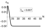
(a)

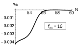
(b)

Figure 1: Evolution of $n_{\delta b}$ some efolds before the end of inflation in two different models. The values of $f_{\rm NL}$ shown are estimated at the end of inflation.

Conclusions.—The halo bias is known to inherit a scale dependence from the underlying inflationary model. It is therefore an important observable which is likely to be measured by future surveys of the galaxy distribution. In this Letter we focus on its scaling, for which we do not require detailed knowledge of the amplitude $A_{\mathrm{NL}}$. We provide a formula to compute $n_{\delta b}$ for any model of multiple-field inflation. To obtain a significant effect, the squeezed limit (characterized by the spectral index $n_{\text{\text{sq}}}$) should scale differently to the power spectrum (characterized by $n_{s}-1$). This can be measured most easily when $n_{\delta b}<0$, making $k^{-2+n_{\delta b}}$ diverge more strongly in the limit $k\rightarrow 0$. Therefore, a slightly red-tilted bias will be easier to constrain than a blue-tilted one.

The principal drawback of our method is the use of a spectral index to parametrize the behavior of the squeezed bispectrum. For a sufficiently large variation of $k_{\text{{l}}}$ the bispectrum may have a shape which cannot be approximated by a power law. Nevertheless, our formula should give a good approximation provided the hierarchy $\ln(k_{\text{{l}}}/k_{\text{{s}}})$ does not exceed $\sim$ a few. Near-future surveys such as DES may probe a hierarchy of order $\ln(k_{\text{{l}}}/k_{\text{{s}}})\sim-2$, but surveys arriving in the medium- to long-term, such as Euclid, may probe $\ln(k_{\text{{l}}}/k_{\text{{s}}})\sim-8$. Small-scale observables such as $\mu$-distortions may even probe $\ln(k_{\text{{l}}}/k_{\text{{s}}})\sim-19$. For such cases a more precise description of the bispectrum will be required, perhaps using numerical methods.

We thank Chris Byrnes, Cora Dvorkin, Simone Ferraro, Jonathan Frazer and Daan Meerburg for discussions. DS and MD acknowledge support from STFC [grant number ST/ I000976/1] and the Leverhulme Trust. DS acknowledges that this material is based upon work supported in part by the NSF under Grant No. 1066293 and the hospitality of the Aspen Center for Physics. The research leading to these results has received funding from the ERC under the European Union’s Seventh Framework Programme (FP/2007–2013)/ERC Grant Agreement No. [308082].

References

- Amendola et al. [2012] L. Amendola et al. (Euclid Theory Working Group), (2012), arXiv:1206.1225 [astro-ph.CO] .
- Ivezic et al. [2008] Z. Ivezic, J. Tyson, R. Allsman, J. Andrew, and R. Angel (LSST Collaboration), (2008), arXiv:0805.2366 [astro-ph] .
- Kogut et al. [2011] A. Kogut, D. Fixsen, D. Chuss, J. Dotson, E. Dwek, et al., JCAP 1107, 025 (2011), arXiv:1105.2044 [astro-ph.CO] .
- LoVerde et al. [2008] M. LoVerde, A. Miller, S. Shandera, and L. Verde, JCAP 0804, 014 (2008), arXiv:0711.4126 [astro-ph] .
- Sefusatti et al. [2009] E. Sefusatti, M. Liguori, A. P. Yadav, M. G. Jackson, and E. Pajer, JCAP 0912, 022 (2009), arXiv:0906.0232 [astro-ph.CO] .
- Giannantonio et al. [2012] T. Giannantonio, C. Porciani, J. Carron, A. Amara, and A. Pillepich, Mon.Not.Roy.Astron.Soc. 422, 2854 (2012), arXiv:1109.0958 [astro-ph.CO] .
- Becker et al. [2012] A. Becker, D. Huterer, and K. Kadota, JCAP 1212, 034 (2012), arXiv:1206.6165 [astro-ph.CO] .
- Becker and Huterer [2012] A. Becker and D. Huterer, Phys.Rev.Lett. 109, 121302 (2012), arXiv:1207.5788 [astro-ph.CO] .
- Shandera et al. [2011] S. Shandera, N. Dalal, and D. Huterer, JCAP 1103, 017 (2011), arXiv:1010.3722 [astro-ph.CO] .
- Sheth and Tormen [2002] R. K. Sheth and G. Tormen, Mon.Not.Roy.Astron.Soc. 329, 61 (2002), arXiv:astro-ph/0105113 [astro-ph] .
- Dalal et al. [2008] N. Dalal, O. Doré, D. Huterer, and A. Shirokov, Phys.Rev. D77, 123514 (2008), arXiv:0710.4560 [astro-ph] .
- Slosar et al. [2008] A. Slosar, C. Hirata, U. Seljak, S. Ho, and N. Padmanabhan, JCAP 0808, 031 (2008), arXiv:0805.3580 [astro-ph] .
- Matarrese and Verde [2008] S. Matarrese and L. Verde, Astrophys.J. 677, L77 (2008), arXiv:0801.4826 [astro-ph] .
- Note [1] There is a correction to Eq. (1\@@italiccorr) proportional to of the integral, obtained in Refs. [47, 48, 49]. This correction will be suppressed relative to the term retained in (1\@@italiccorr) by a term proportional to the departure of and from scale-invariance, and will therefore be small when the spectrum and bispectrum are nearly scale-invariant.
- Afshordi and Tolley [2008] N. Afshordi and A. J. Tolley, Phys.Rev. D78, 123507 (2008), arXiv:0806.1046 [astro-ph] .
- Verde and Matarrese [2009] L. Verde and S. Matarrese, Astrophys.J. 706, L91 (2009), arXiv:0909.3224 [astro-ph.CO] .
- Ade et al. [2013] P. Ade et al. (Planck Collaboration), (2013), arXiv:1303.5084 [astro-ph.CO] .
- Sefusatti et al. [2012] E. Sefusatti, J. R. Fergusson, X. Chen, and E. Shellard, JCAP 1208, 033 (2012), arXiv:1204.6318 [astro-ph.CO] .
- Biagetti et al. [2013] M. Biagetti, H. Perrier, A. Riotto, and V. Desjacques, (2013), arXiv:1301.2771 [astro-ph.CO] .
- Chen [2005] X. Chen, Phys.Rev. D72, 123518 (2005), arXiv:astro-ph/0507053 [astro-ph] .
- Byrnes et al. [2010] C. T. Byrnes, M. Gerstenlauer, S. Nurmi, G. Tasinato, and D. Wands, JCAP 1010, 004 (2010), arXiv:1007.4277 [astro-ph.CO] .
- Byrnes and Gong [2013] C. T. Byrnes and J.-O. Gong, Phys.Lett. B718, 718 (2013), arXiv:1210.1851 [astro-ph.CO] .
- Tzavara and van Tent [2012] E. Tzavara and B. van Tent, (2012), arXiv:1211.6325 [astro-ph.CO] .
- Sasaki and Stewart [1996] M. Sasaki and E. D. Stewart, Prog.Theor.Phys. 95, 71 (1996), arXiv:astro-ph/9507001 [astro-ph] .
- Dias and Seery [2012] M. Dias and D. Seery, Phys.Rev. D85, 043519 (2012), arXiv:1111.6544 [astro-ph.CO] .
- Note [2] See Ref. [50] for an earlier application of a similar method.
- Nakamura and Stewart [1996] T. T. Nakamura and E. D. Stewart, Phys.Lett. B381, 413 (1996), arXiv:astro-ph/9604103 [astro-ph] .
- Avgoustidis et al. [2012] A. Avgoustidis, S. Cremonini, A.-C. Davis, R. H. Ribeiro, K. Turzyński, et al., JCAP 1202, 038 (2012), arXiv:1110.4081 [astro-ph.CO] .
- Seery et al. [2012] D. Seery, D. J. Mulryne, J. Frazer, and R. H. Ribeiro, JCAP 1209, 010 (2012), arXiv:1203.2635 [astro-ph.CO] .
- Chen et al. [2007] X. Chen, M.-x. Huang, S. Kachru, and G. Shiu, JCAP 0701, 002 (2007), arXiv:hep-th/0605045 [hep-th] .
- Burrage et al. [2011] C. Burrage, R. H. Ribeiro, and D. Seery, JCAP 1107, 032 (2011), arXiv:1103.4126 [astro-ph.CO] .
- Ribeiro [2012] R. H. Ribeiro, JCAP 1205, 037 (2012), arXiv:1202.4453 [astro-ph.CO] .
- Dias et al. [2012] M. Dias, R. H. Ribeiro, and D. Seery, (2012), arXiv:1210.7800 [astro-ph.CO] .
- Creminelli et al. [2011] P. Creminelli, G. D’Amico, M. Musso, and J. Noreña, JCAP 1111, 038 (2011), arXiv:1106.1462 [astro-ph.CO] .
- Lyth and Zaballa [2005] D. H. Lyth and I. Zaballa, JCAP 0510, 005 (2005), arXiv:astro-ph/0507608 [astro-ph] .
- Vernizzi and Wands [2006] F. Vernizzi and D. Wands, JCAP 0605, 019 (2006), arXiv:astro-ph/0603799 [astro-ph] .
- Mulryne et al. [2010] D. J. Mulryne, D. Seery, and D. Wesley, JCAP 1001, 024 (2010), arXiv:0909.2256 [astro-ph.CO] .
- Mulryne et al. [2011] D. J. Mulryne, D. Seery, and D. Wesley, JCAP 1104, 030 (2011), arXiv:1008.3159 [astro-ph.CO] .
- Anderson et al. [2012] G. J. Anderson, D. J. Mulryne, and D. Seery, JCAP 1210, 019 (2012), arXiv:1205.0024 [astro-ph.CO] .
- Elliston et al. [2012a] J. Elliston, D. Seery, and R. Tavakol, JCAP 1211, 060 (2012a), arXiv:1208.6011 [astro-ph.CO] .
- Mulryne [2013] D. J. Mulryne, (2013), arXiv:1302.3842 [astro-ph.CO] .
- Silk and Turner [1987] J. Silk and M. S. Turner, Phys.Rev. D35, 419 (1987).
- Polarski and Starobinsky [1994] D. Polarski and A. A. Starobinsky, Phys.Rev. D50, 6123 (1994), arXiv:astro-ph/9404061 [astro-ph] .
- García-Bellido and Wands [1996] J. García-Bellido and D. Wands, Phys.Rev. D53, 5437 (1996), arXiv:astro-ph/9511029 [astro-ph] .
- Langlois [1999] D. Langlois, Phys.Rev. D59, 123512 (1999), arXiv:astro-ph/9906080 [astro-ph] .
- Elliston et al. [2012b] J. Elliston, L. Alabidi, I. Huston, D. Mulryne, and R. Tavakol, JCAP 1209, 001 (2012b), arXiv:1203.6844 [astro-ph.CO] .
- Desjacques et al. [2011] V. Desjacques, D. Jeong, and F. Schmidt, Phys.Rev. D84, 063512 (2011), arXiv:1105.3628 [astro-ph.CO] .
- Adshead et al. [2012] P. Adshead, E. J. Baxter, S. Dodelson, and A. Lidz, Phys.Rev. D86, 063526 (2012), arXiv:1206.3306 [astro-ph.CO] .
- Baumann et al. [2012] D. Baumann, S. Ferraro, D. Green, and K. M. Smith, (2012), arXiv:1209.2173 [astro-ph.CO] .
- Byrnes and Wands [2006] C. T. Byrnes and D. Wands, Phys.Rev. D74, 043529 (2006), arXiv:astro-ph/0605679 [astro-ph] .