Inflation and deformation of conformal field theory

Abstract:

It has recently been suggested that a strongly coupled phase of inflation may be described holographically in terms of a weakly coupled quantum field theory (QFT). Here, we explore the possibility that the wave function of an inflationary universe may be given by the partition function of a boundary QFT. We consider the case when the field theory is a small deformation of a conformal field theory (CFT), by the addition of a relevant operator $O$, and calculate the primordial spectrum predicted in the corresponding holographic inflation scenario. Using the Ward-Takahashi identity associated with Weyl rescalings, we derive a simple relation between correlators of the curvature perturbation $\zeta$ and correlators of the deformation operator $O$ at the boundary. This is done without specifying the bulk theory of gravitation, so that the result would also apply to cases where the bulk dynamics is strongly coupled. We comment on the validity of the Suyama-Yamaguchi inequality, relating the bi-spectrum and tri-spectrum of the curvature perturbation.

1 Introduction

The inflationary paradigm is very successful in explaining the initial conditions of our Big Bang universe. Inflation can be driven by a light scalar field slowly rolling down a potential, and in this case the quantum fluctuations of the scalar field may yield a primordial source of the later structure formation. To verify inflation, and perhaps uncover a more concrete realization of it, it is important to analyze the predicted primordial fluctuations in different models, so they can be compared with observations [1].

In the conventional approach, models of inflation are investigated under the assumption that the fields are weakly coupled, so that their quantum effects can be perturbatively examined. However, since inflation is expected to take place at a high energy scale, this assumption may not be realized. The gauge/gravity duality [2, 3, 4] states that the dynamics of asymptotically AdS spacetimes is dual to a CFT at its conformal boundary. AdS/CFT relates weak coupling on one side of the duality to strong coupling in the other side. As it stands, such duality cannot be applied to inflationary cosmology, where the spacetime is similar to de Sitter rather than AdS. Nonetheless, by analogy, there have been several suggestions that a $(d+1)$-dimensional inflationary evolution may be dual to a quantum field theory (QFT) on a $d$-dimensional space of Euclidean signature. Following the work by Strominger [5, 6] and Witten [7], the possible duality between gravity in de Sitter space and a CFT has been investigated in Refs. [8, 9, 10]. A holographic description of quasi-de Sitter spacetime would provide a new approach for analyzing the origin of cosmological perturbations [6, 11, 12], allowing us to consider a strongly coupled phase of inflation. This would correspond to the weakly coupled phase of the boundary theory, which can be treated perturbatively.

McFadden and Skenderis [13, 14, 15, 16, 17, 18] have recently focused on the so-called domain wall/cosmology correspondence. This is based on the observation that domain wall solutions can be mapped into cosmological solutions by analytic continuation [19, 20]. First they describe the gravitational field of the domain wall solution in terms of the dual QFT on the boundary based on the gauge/gravity duality, using the holographic renormalization group method [21, 22, 23]. Then, they perform the analytic continuation to transform the domain wall solution into the cosmological spacetime solution. Skenderis and McFadden show that the mapping can be extended to include cosmological perturbations. The results presented in Refs. [13, 14, 15, 16, 17, 18] are rather robust and amenable to comparison with upcoming cosmological observations [15, 24, 25].

Motivated by these developments, we further investigate the holographic description of the inflationary spacetime. Here, we take as our starting point the assumption that the wave function of the $(d+1)$-dimensional bulk gravitational field of the inflationary spacetime is given by the generating functional of the dual QFT on the $d$-dimensional boundary [6, 7, 11, 26]. (See also Refs. [27, 28].) The bulk dynamics is then supposed to be dual to a QFT on the Euclidean boundary and the RG flow describes the bulk evolution. Under this assumption, we will formally derive the relation between the primordial fluctuation in the bulk inflationary spacetime and the dual QFT on the boundary. To introduce a deviation from the exact de Sitter symmetry in the bulk, we will consider a deformation of the CFT on the boundary. Our approach is manifestly independent of the bulk dynamics. Rather, the theory is defined in terms of the dual QFT.

The outline of this paper is as follows. In Sec. 2, we describe our setup. In Sec. 3, using the Ward-Takahashi identity associated with the Weyl transformation, we derive the relation between the wave function and the boundary QFT operators. In Sec. 4, using the formulas derived in the preceding sections, we give the formal expression of the primordial spectra described by the correlation functions of the boundary QFT operators. We also investigate the validity of the Suyama-Yamaguchi inequality, which is known to hold for a wide class of weakly coupled inflation models.

2 Preliminaries

The cosmological spacetime metric can be given in ADM formalism as

$${\rm d}s^{2}=-N^{2}{\rm d}t^{2}+h_{ij}\left({\rm d}x^{i}+N^{i}{\rm d}t\right)\left({\rm d}x^{j}+N^{j}{\rm d}t\right)\,.$$ (1)

Here we shall restrict attention to the situation where the metric is asymptotically de Sitter. In the semiclassical picture, this would correspond to the case a period of slow roll inflation is followed by $\Lambda$ domination. In this case, the future conformal boundary is space-like and will be thought of as home to a QFT.

Our starting point is the assumption that the wave function of the bulk gravitational field is related to the generating functional of the boundary QFT

$$\psi_{\rm bulk}[h,\phi]\propto Z_{\rm QFT}[h,\phi]\,,$$ (2)

where the generating functional $Z_{\rm QFT}$ is given by

$$Z_{\rm QFT}[h,\phi]=e^{-W_{\rm QFT}[h,\phi]}=\int D\chi\,\exp\left(-S_{\rm QFT}[\chi,\,h,\,\phi]\right)\,.$$ (3)

Here $\psi_{\rm bulk}$ denotes the wave function of the bulk and $\chi$ denotes boundary fields, for which the metric $h_{ij}$ and the inflaton $\phi$ act as sources (the indices in $h_{ij}$ will be omitted when unnecessary). Note that $h$ and $\phi$ correspond to the values of the metric and inflaton at the future boundary, where any finite co-moving separation corresponds to an infinite physical wavelength in the bulk theory.

Since the wave function $\psi_{\rm bulk}$ is generally complex, $W_{\rm QFT}$ will have real and imaginary part, which means that this is not the effective action of a standard unitary Euclidean field theory. In the regime where gravity is semiclassical, we have

$$\psi_{\rm bulk}\approx|\psi_{\rm bulk}|e^{iS_{\rm bulk}},$$ (4)

where $S_{\rm bulk}$ is the classical bulk action as a function of the boundary fields. For long wavelength modes, the modulus is approximately constant in time, while the classical action $S_{\rm bulk}$ is extensive in the space-time volume and grows unbounded with the scale factor $a$. In the dual picture, the scale factor will play the role of the renormalization scale $\mu$, so the divergent terms in $W_{\rm QFT}$ are in fact purely imaginary. Because of that, some imaginary counterterms will be necessary in $S_{\rm QFT}$, and one may prefer to define the generating functional as [29]

$$Z_{\rm QFT}=e^{i\bar{W}_{\rm QFT}}=\int D\chi\,\exp\left(i\bar{S}_{\rm QFT}[\chi,\,h,\,\phi]\right),$$ (5)

where

$$\bar{W}_{\rm QFT}=iW_{\rm QFT},\ \quad\quad\bar{S}_{\rm QFT}=iS_{\rm QFT}.$$ (6)

In this notation, the counterterms in $\bar{S}_{\rm QFT}$ would be purely real. Here, we will simply follow the notation in Ref. [30], where Eq.(3) is used with the understanding that $S_{\rm QFT}$ is necessarily complex. The interchange between the two notations is of course trivial.

2.1 Deformed CFT

We shall concentrate on the case where the QFT is a small deformation of a CFT with

$$S_{u}[\chi]=S_{\rm CFT}[\chi]+\int{\rm d}^{d}\hbox{\boldmath{$x$}}\sqrt{h}\,u\,O(\hbox{\boldmath{$x$}})\,.$$ (7)

The first term preservers the conformal symmetry, and $O(\hbox{\boldmath{$x$}})$ is a QFT operator with the scaling dimension $\Delta$. Introducing

$$\lambda\equiv\Delta-d\,,$$ (8)

the case $\lambda=0$ corresponds to a marginal deformation, which changes the theory into another CFT. An operator with $\lambda>0$ corresponds to an irrelevant deformation and an operator with $\lambda<0$ corresponds to a relevant deformation [31]. An operator with $\lambda\neq 0$ introduces a renormalization group flow which is characterized by the beta function. This is defined for a dimensionless coupling constant

$$g(\mu)\equiv\mu^{\lambda_{c}}u(\mu)$$ (9)

as

$$\beta\equiv\frac{{\rm d}g(\mu)}{{\rm d}\ln\mu}\,,$$ (10)

where $\mu$ is the energy scale and we have introduced

$$\lambda_{c}\equiv\delta-d\,.$$ (11)

Here, $\delta$ is the classical scaling dimension, which is in general different from $\Delta$. Noticing the fact that the coupling always appears in the combination $\mu^{-\lambda_{c}}g(\mu)$ in the classical action, we can express the beta function as

$$\beta=\lambda_{c}g+\beta^{\rm quant}\,,$$ (12)

where integrating the quantum corrections gives rise to the deviation from the classical scaling. We assume that the theory approaches a fixed point at high energies, so that $u$ approaches 0. Conformal symmetry is then recovered. The coupling constant $g$ of the boundary theory is interpreted as the boundary value of the inflaton $\phi$,

$$g=\phi/M_{\rm pl}$$ (13)

where we divided the inflaton by the Planck scale $M_{\rm pl}$ to keep $g$ dimensionless.

If the energy scale $\mu$ is identified with the cosmological scale factor $\mu\propto a$, we can rewrite the beta function as $\beta\simeq({\rm d}/{\rm d}\ln a)\phi/M_{\rm pl}$. Once we assume the field equation for the bulk gravitational field, we can express the deformation parameters $\lambda$ and $\beta$ in terms of the so-called slow-roll parameters, which describe the deviation from the exact de Sitter space. For instance, using the Friedmann equation, we can express $\beta$ in terms of the slow-roll parameter $\varepsilon\equiv H({\rm d}/{\rm d}\ln a)1/H$ as $\beta^{2}\propto\varepsilon$ [26, 27]. However, in the strongly coupled limit of bulk gravity, such relations need not apply. In this paper, we will not make any reference to bulk equations of motion. Our arguments are based on the assumption that the boundary theory is dual to the (perhaps strongly coupled) bulk theory through Eq. (2). This provides a direct relation between the long wavelength correlators of the bulk gravitational field and the correlators of the field theory operator $O$. The parameters $\beta$ and $\lambda$ will be fixed by solving the RG flow from the UV fixed point to the IR fixed point [18, 32]. Since our aim is to give a formal expression of the primordial spectrum in terms of boundary QFT operators, we simply assume that $\beta$ and $\lambda$ are given functions of the energy scale.

2.2 The wave function

Throughout this paper, we shall restrict attention to the scalar component of the boundary fields $h_{ij}$ and $\phi$. In a bulk description, we adopt the gauge condition $\delta\phi=0$ and

$$h_{ij}=a^{2}(t)e^{2\zeta}\delta_{ij}\,,$$ (14)

where we neglected the tensor modes. We normalize the scale factor $a(t)$ as $a(t_{c})=1$ where $t_{c}$ is the coordinate $t$ which corresponds to the UV cutoff scale of QFT. In the following, we calculate the primordial fluctuation at a fixed probe brane with $t=t_{c}$. For notational simplicity, we abbreviate the coordinate $t$ in the arguments of fields.

From (3), we have

$$\psi_{\rm bulk}[\zeta]=A\,Z_{\rm QFT}[\zeta]=A\,e^{-W_{\rm QFT}[\zeta]}\,,$$ (15)

where we wrote a normalization constant $A$ explicitly. We may now calculate $n$-point functions of the gravitational field perturbation in terms of the QFT correlators. From the wave function $\psi_{\rm bulk}[\zeta]$, we obtain the probability density

$$P[\zeta]=\left|\psi_{\rm bulk}[\zeta]\right|^{2}=|A|^{2}\,e^{-(W_{\rm QFT}[\zeta]+W_{\rm QFT}^{*}[\zeta])}\,.$$ (16)

Once we obtain the probability density function $P[\zeta]$, we can calculate the $n$-point functions for $\zeta$ on the boundary as

$$\langle\zeta(\hbox{\boldmath{$x$}}_{1})\zeta(\hbox{\boldmath{$x$}}_{2})\cdots\zeta(\hbox{\boldmath{$x$}}_{n})\rangle=\int D\zeta\,P[\zeta]\,\zeta(\hbox{\boldmath{$x$}}_{1})\zeta(\hbox{\boldmath{$x$}}_{2})\cdots\zeta(\hbox{\boldmath{$x$}}_{n})$$ (17)

where $D\zeta$ is the integration measure. In weakly coupled Einstein gravity, the bulk distribution is given by a nearly Gaussian distribution for the variable $\zeta$, accompanied by a measure which is linear in $\zeta$. On the other hand, our aim here is to proceed without reference to the explicit form of the bulk theory. Hence, after postulating the correspondence (15) for the wave function, we still need some justification for choosing $D\zeta$ instead of, say, $Df(\zeta)$, where $f$ is an arbitrary function. As we shall see, the holographic distribution (16) becomes independent of $\zeta$ as we approach the conformal fixed point. This limit corresponds to de Sitter space, where the variable $\zeta$ is pure gauge. We therefore expect that all values of $\zeta$ should become equally probable as the conformal fixed point is approached. This will only be realized if we choose $f$ to be linear in $\zeta$. In this case, the measure is invariant under the Weyl rescalings, since as we will see in the next section, the Weyl rescalings simply shift $\zeta$ as $\zeta\to\zeta-\alpha$, where $\alpha$ is an arbitrary function of position.

We determine the normalization constant $A$, adopting the normalization condition:

$$\int D\zeta P[\zeta]=1\,.$$ (18)

Eliminating the background contribution $W_{\rm QFT}[\zeta=0]$ by the redefinition of $A$, $P[\zeta]$ is given by

$$P[\zeta]=|A|^{2}e^{-\zeta\cdot W^{(1)}-\frac{1}{2}\zeta\cdot W^{(2)}\cdot\zeta-\delta W_{\rm NL}[\zeta]}\,,$$ (19)

where we defined the vertex function $W^{(n)}(\hbox{\boldmath{$x$}}_{1},\,\cdots,\,\hbox{\boldmath{$x$}}_{n})$ for $n\geq 1$ as

$$W^{(n)}(\hbox{\boldmath{$x$}}_{1},\,\cdots,\,\hbox{\boldmath{$x$}}_{n})\equiv 2\,{\rm Re}\left[\frac{\delta^{n}W_{\rm QFT}[\zeta]}{\delta\zeta(\hbox{\boldmath{$x$}}_{1})\cdots\delta\zeta(\hbox{\boldmath{$x$}}_{n})}\right]\,.$$ (20)

For a later use, we discriminated the non-linear interactions, introducing $\delta W_{\rm NL}[\zeta]$ which is defined as

$$\delta W_{\rm NL}[\zeta]\equiv\sum_{n=3}\frac{1}{n!}\int{\rm d}^{d}\hbox{\boldmath{$x$}}_{1}\cdots\int{\rm d}^{d}\hbox{\boldmath{$x$}}_{n}\,W^{(n)}(\hbox{\boldmath{$x$}}_{1},\,\cdots\,,\hbox{\boldmath{$x$}}_{n})\zeta(\hbox{\boldmath{$x$}}_{1})\cdots\zeta(\hbox{\boldmath{$x$}}_{n})\,.$$ (21)

Here and hereafter we use an abbreviated notation:

$$\phi\cdot\psi\equiv\int{\rm d}^{d}\hbox{\boldmath{$x$}}\phi(\hbox{\boldmath{$x$}})\psi(\hbox{\boldmath{$x$}})\,,$$ (22)

$$\phi\cdot M\cdot\psi\equiv\int{\rm d}^{d}\hbox{\boldmath{$x$}}_{1}\!\int\!{\rm d}^{d}\hbox{\boldmath{$x$}}_{2}\,\phi(\hbox{\boldmath{$x$}}_{1})M(\hbox{\boldmath{$x$}}_{1},\,\hbox{\boldmath{$x$}}_{2})\psi(\hbox{\boldmath{$x$}}_{2})\,$$ (23)

for functions $\phi(\hbox{\boldmath{$x$}})$ and $\psi(\hbox{\boldmath{$x$}})$ and a matrix function $M(\hbox{\boldmath{$x$}}_{1},\,\hbox{\boldmath{$x$}}_{2})$.

First, we consider the case with $W^{(1)}(\hbox{\boldmath{$x$}})=0$. In deriving the $n$-point functions for $\zeta$, it is convenient to perform the Legendre transform as

$$\Phi[J]\equiv\int D\zeta\,P[\zeta]e^{-\zeta\cdot J}=|A|^{2}\int D\zeta\,e^{-\frac{1}{2}\zeta\cdot W^{(2)}\cdot\zeta-\delta W_{\rm NL}[\zeta]-\zeta\cdot J}\,.$$ (24)

We can easily understand that $n$-th derivatives of $\Phi[J]$ in terms of $J(\hbox{\boldmath{$x$}})$ yield $n$-point functions of $\zeta(\hbox{\boldmath{$x$}})$. Using the generating functional for the free field given by

$$\Phi_{0}[J]=|A|^{2}\int D\zeta\,e^{-\frac{1}{2}\zeta\cdot W^{(2)}\cdot\zeta-\zeta\cdot J}=|A|^{2}\,e^{\frac{1}{2}J\cdot W^{(2)\,-1}\cdot J}\,,$$ (25)

where $W^{(2)\,-1}(\hbox{\boldmath{$x$}}_{1},\,\hbox{\boldmath{$x$}}_{2})$ is the inverse matrix of $W^{(2)}(\hbox{\boldmath{$x$}}_{1},\,\hbox{\boldmath{$x$}}_{2})$, which satisfies

$$\int{\rm d}^{d}\hbox{\boldmath{$x$}}\,W^{(2)}(\hbox{\boldmath{$x$}}_{1},\,\hbox{\boldmath{$x$}})W^{(2)\,-1}(\hbox{\boldmath{$x$}},\,\hbox{\boldmath{$x$}}_{2})=\delta(\hbox{\boldmath{$x$}}_{1}-\hbox{\boldmath{$x$}}_{2})\,,$$ (26)

the generating functional $\Phi[J]$ is recast into

$$\Phi[J] =e^{-\delta W_{\rm NL}[\delta/\delta J]}\,\Phi_{0}[J]=|A|^{2}e^{-\delta W_{\rm NL}[\delta/\delta J]}\,e^{\frac{1}{2}J\cdot W^{(2)\,-1}\cdot J}$$ (27)

$$=|A|^{2}e^{\frac{1}{2}\delta/\delta\zeta\cdot W^{(2)\,-1}\cdot\delta/\delta\zeta}e^{-\delta W_{\rm NL}[\zeta]-\zeta\cdot J}\Big{|}_{\zeta=0}\,.$$ (28)

On the last equality, we used the following identity:

$$F[\delta/\delta\zeta]G[\zeta]e^{-\zeta\cdot J}\big{|}_{\zeta=0}=G[\delta/\delta(-J)]F[-J]\,,$$ (29)

which is valid for arbitrary functionals $F$ and $G$. Substituting $|A|$ which is determined by the normalization condition (18), the generating functional $\Phi[J]$ is finally given by

$$\Phi[J]=\frac{e^{\frac{1}{2}\delta/\delta\zeta\cdot W^{(2)\,-1}\cdot\delta/\delta\zeta}e^{-\delta W_{\rm NL}[\zeta]-\zeta\cdot J}\big{|}_{\zeta=0}}{e^{\frac{1}{2}\delta/\delta\zeta\cdot W^{(2)\,-1}\cdot\delta/\delta\zeta}e^{-\delta W_{\rm NL}[\zeta]}\big{|}_{\zeta=0}}\,.$$ (30)

This formula can be understood as follows. We first expand the exponential terms $e^{-\delta W_{\rm NL}[\zeta]-\zeta\cdot J}$ up to a desired order in perturbation. A coefficient of a term with $J(\hbox{\boldmath{$x$}}_{1})\cdots J(\hbox{\boldmath{$x$}}_{n})$ gives the $n$-point function for $\zeta$. These correlators can be evaluated after we multiply the derivative operator $e^{\frac{1}{2}\delta/\delta\zeta\cdot W^{(2)\,-1}\cdot\delta/\delta\zeta}$, which replaces two $\zeta$s with $W^{(2)\,-1}$. Since we set $\zeta=0$ after this replacement, only terms with an even number of $\zeta$s can survive. We can derive the Feynman rules as in the path integral of a usual quantum field theory. The only difference is that, in the present case, the vertices $W^{(n)}$ are generically non-local, depending on $n$ separate points $\hbox{\boldmath{$x$}}_{i}$ which are integrated over. Different ways of taking derivatives by $\delta/\delta\zeta$ correspond to different diagrams. In the diagrammatic description, the non-locality of the vertices can be illustrated by splitting the interaction point into $n$ separated ones, as in Figs. 1 and 2. The generating functional $\Phi[J]$ for the case with $W^{(1)}\neq 0$ can be obtained simply by replacing $\delta W_{\rm NL}[\zeta]$ with $\delta W_{\rm NL}[\zeta]+W^{(1)}\cdot\zeta$ in the exponents of Eq. (30). Following the conventional quantum field theory, to pick up only connected diagrams, we define the $n$-point functions as

$$\langle\zeta(\hbox{\boldmath{$x$}}_{1})\cdots\zeta(\hbox{\boldmath{$x$}}_{n})\rangle_{\rm conn}\equiv(-1)^{n}\frac{\delta^{n}}{\delta J(\hbox{\boldmath{$x$}}_{1})\cdots\delta J(\hbox{\boldmath{$x$}}_{n})}\ln\Phi[J]\bigg{|}_{J=0}\,\,,$$ (31)

where we put the suffix “conn” to emphasize including only connected diagrams.

3 Derivatives of the generating functional

In this section, using the Ward-Takahashi identity associated with the Weyl transformation, we express the vertex function $W^{(n)}(\hbox{\boldmath{$x$}}_{1},\,\cdots,\,\hbox{\boldmath{$x$}}_{n})$ in terms of field theory correlators. The classical scalings of the metric $g_{ij}$ and the operator $O$ are given by

$$g_{ij}(\hbox{\boldmath{$x$}})\to e^{-2\alpha(\hbox{\boldmath{\scriptsize$x$}})}g_{ij}(\hbox{\boldmath{$x$}})\,,\qquad O(\hbox{\boldmath{$x$}})\to e^{\Delta\alpha(\hbox{\boldmath{\scriptsize$x$}})}O(\hbox{\boldmath{$x$}})\equiv O_{\alpha}(\hbox{\boldmath{$x$}})\,.$$ (32)

In the gauge with Eq. (14), the Weyl transformation of the metric is expressed as

$$\zeta(\hbox{\boldmath{$x$}})\to\zeta(\hbox{\boldmath{$x$}})-\alpha(\hbox{\boldmath{$x$}})\equiv\zeta_{\alpha}(\hbox{\boldmath{$x$}})\,.$$ (33)

In the following, we will show that the generating functional $W_{\rm QFT}[\zeta]$ and also the vertex function $W^{(n)}(\hbox{\boldmath{$x$}}_{1},\,\cdots,\,\hbox{\boldmath{$x$}}_{n})$ are related to correlation functions of $O$ by a simple relation. Since we fixed the slicing of the $t$-constant surface requesting $\delta\phi=0$, the coupling constant $u$ is homogeneous and will not be affected by the Weyl transformation.

3.1 The Ward-Takahashi identity

Under the Weyl transformation (32), the action $S_{u}$ transforms as

$$S_{u}[\zeta,\,\chi]\to S_{u}[\zeta_{\alpha},\,\chi_{\alpha}] =S_{\rm CFT}[\zeta_{\alpha},\,\chi_{\alpha}]+\int{\rm d}^{d}\hbox{\boldmath{$x$}}e^{d\zeta_{\alpha}(\hbox{\boldmath{\scriptsize$x$}})}u\,O_{\alpha}(\hbox{\boldmath{$x$}})$$ (34)

$$=S_{\rm CFT}[\zeta,\,\chi]+\int{\rm d}^{d}\hbox{\boldmath{$x$}}e^{d\zeta(\hbox{\boldmath{\scriptsize$x$}})}e^{(\Delta-d)\alpha(\hbox{\boldmath{\scriptsize$x$}})}u\,O(\hbox{\boldmath{$x$}})$$ (35)

$$=S_{u}[\zeta,\,\chi]+\delta S_{\alpha}[\zeta,\,\chi]\,,$$ (36)

where we defined

$$\delta S_{\alpha}[\zeta,\,\chi]\equiv\int{\rm d}^{d}\hbox{\boldmath{$x$}}e^{d\zeta(\hbox{\boldmath{\scriptsize$x$}})}\left[e^{\lambda\alpha(\hbox{\boldmath{\scriptsize$x$}})}-1\right]u\,O(\hbox{\boldmath{$x$}})\,.$$ (37)

On the second equality, we noted that $S_{\rm CFT}$ is invariant under the Weyl transformation. (The conformal invariance only implies the invariance under the Weyl transformation with the specific $x$-dependent parameter $\alpha(\hbox{\boldmath{$x$}})$. To be more precise, $S_{\rm CFT}$ is assumed to preserve the Weyl invariance rather than the conformal symmetry.) Noticing the fact that the integration of the generating functional is independent of the choice of integration variable, we express $Z_{\rm QFT}$ as

$$Z_{\rm QFT}=\int D\chi\,e^{-S_{u}[\zeta_{\alpha},\,\chi]}=\int D\chi_{\alpha}\,e^{-S_{u}[\zeta_{\alpha},\,\chi_{\alpha}]}\,.$$ (38)

Using Eq. (36), we can rewrite this relation as

$$\int D\chi\,e^{-S_{u}[\zeta-\alpha,\,\chi]}=\int D\chi\,{\cal J}[\alpha]e^{-\{S_{u}[\zeta,\,\chi]+\delta S_{\alpha}[\zeta,\,\chi]\}}\,,$$ (39)

where ${\cal J}[\alpha]$ denotes the Jacobian of the integration measure, i.e., $D\chi_{\alpha}={\cal J}[\alpha]D\chi$. Equation (39) provides the so-called Ward-Takahashi identity associated with the Weyl transformation.

The Jacobian ${\cal J}[\alpha]$ can be obtained by considering the transformation of the boundary fields $\chi$ under the Weyl transformation. A change of the integration measure $D\chi$ is known to yield the Weyl anomaly (see for instance Ref. [33]). In odd dimensions, we can employ ${\cal J}[\alpha]=1$, since the Weyl anomaly is absent. In even dimensions, since the anomaly is present, ${\cal J}[\alpha]$ can be different from 1 (see for instance Ref. [34] and references therein). Therefore, here, we focus on odd dimensions with ${\cal J}[\alpha]=1$, leaving a study of the case with ${\cal J}[\alpha]\neq 1$ for future issue.

Next, we operate $\delta^{n}/\delta\alpha(\hbox{\boldmath{$x$}}_{1})\cdots\delta\alpha(\hbox{\boldmath{$x$}}_{n})$ on the both sides of Eq. (39) and set all $\alpha(\hbox{\boldmath{$x$}})$s to $0$. Noticing the fact that the path integral of the left-hand side of Eq. (39) includes $\alpha(\hbox{\boldmath{$x$}})$ only in the form of $\zeta(\hbox{\boldmath{$x$}})-\alpha(\hbox{\boldmath{$x$}})$, we can obtain the Ward-Takahashi identity as

$$(-1)^{n}\frac{\delta^{n}}{\delta\zeta(\hbox{\boldmath{$x$}}_{1})\cdots\delta\zeta(\hbox{\boldmath{$x$}}_{n})}\int D\chi\,e^{-S_{u}[\zeta,\,\chi]}$$ (40)

$$\qquad\quad=\frac{\delta^{n}}{\delta\alpha(\hbox{\boldmath{$x$}}_{1})\cdots\delta\alpha(\hbox{\boldmath{$x$}}_{n})}\int D\chi\,e^{-\{S_{u}[\zeta,\,\chi]+\delta S_{\alpha}[\zeta,\,\chi]\}}\bigg{|}_{\alpha=0}\,,$$ (41)

where we noted that since the integration measure does not change under the Weyl transformation induced by a change of $\zeta$, $D\chi$ commutes with $\delta/\delta\zeta$. The left hand side of Eq. (41) is nothing but the differentiation of the generating functional $Z_{\rm QFT}[\zeta]$ in terms of $\zeta(\hbox{\boldmath{$x$}})$. Dividing Eq. (41) by $Z_{\rm QFT}[\zeta]$ and sending $\zeta$ to 0, we obtain

$$\frac{1}{Z_{\rm QFT}[\zeta]}\frac{\delta^{n}}{\delta\zeta(\hbox{\boldmath{$x$}}_{1})\cdots\delta\zeta(\hbox{\boldmath{$x$}}_{n})}Z_{\rm QFT}[\zeta]\bigg{|}_{\zeta=0}=(-1)^{n}\left\langle\frac{\delta^{n}}{\delta\alpha(\hbox{\boldmath{$x$}}_{1})\cdots\delta\alpha(\hbox{\boldmath{$x$}}_{n})}e^{-\delta S_{\alpha}[\zeta,\,\chi]}\bigg{|}_{\alpha=0}\right\rangle_{u}$$ (42)

where we defined

$$\langle X[\chi]\rangle_{u}\equiv\frac{1}{Z_{\rm QFT}[\zeta=0]}\int D\chi\,e^{-S_{u}[\zeta=0,\,\chi]}X[\chi]\,.$$ (43)

To emphasize $u$-dependence, we put the index $u$.

After a straightforward calculation, we can express the right hand side of Eq. (42) in terms of the correlation functions of the QFT operator $O(\hbox{\boldmath{$x$}})$ as

$$\frac{1}{Z_{\rm QFT}[\zeta]}\frac{\delta^{n}}{\delta\zeta(\hbox{\boldmath{$x$}}_{1})\cdots\delta\zeta(\hbox{\boldmath{$x$}}_{n})}Z_{\rm QFT}[\zeta]\bigg{|}_{\zeta=0}$$ (44)

$$\quad=\lambda^{n}\biggl{[}u^{n}\langle O(\hbox{\boldmath{$x$}}_{1})\cdots O(\hbox{\boldmath{$x$}}_{n})\rangle_{u}$$ (45)

$$\qquad\qquad\quad-u^{n-1}\left\{\delta(\hbox{\boldmath{$x$}}_{1}-\hbox{\boldmath{$x$}}_{2})\langle O(\hbox{\boldmath{$x$}}_{2})\cdots O(\hbox{\boldmath{$x$}}_{n})\rangle_{u}+\left(\frac{n(n-1)-2}{2}\,\,{\rm cyclic~{}perms}\right)\right\}$$ (46)

$$\qquad\qquad\quad+\cdots+(-1)^{n-1}u\,\delta(\hbox{\boldmath{$x$}}_{1}-\hbox{\boldmath{$x$}}_{2})\cdots\delta(\hbox{\boldmath{$x$}}_{n-1}-\hbox{\boldmath{$x$}}_{n})\langle O(\hbox{\boldmath{$x$}}_{1})\rangle_{u}\biggr{]}\,.$$ (47)

Using Eq. (20) and dropping the terms which do not contribute to the connected diagram, we obtain the vertex function $W^{(n)}(\hbox{\boldmath{$x$}}_{1},\,\cdots,\,\hbox{\boldmath{$x$}}_{n})$ as

$$W^{(n)}(\hbox{\boldmath{$x$}}_{1},\,\cdots,\,\hbox{\boldmath{$x$}}_{n}) =-2{\rm Re}\left[\frac{1}{Z_{\rm QFT}[\zeta]}\frac{\delta^{n}Z_{\rm QFT}[\zeta]}{\delta\zeta(\hbox{\boldmath{$x$}}_{1})\cdots\delta\zeta(\hbox{\boldmath{$x$}}_{n})}\bigg{|}_{\zeta=0}\right]\,.$$ (48)

In this way, using the Ward-Takahashi identity, the vertex function $W^{(n)}(\hbox{\boldmath{$x$}}_{1},\cdots,\hbox{\boldmath{$x$}}_{n})$ can be expressed in terms of the correlation functions for the QFT operator $O$ and the deformation parameters $\lambda$ and $u$, which characterize the deviation from the conformal fixed point. Note that at the fixed point, where $u$ vanishes, the right-hand side of Eq. (48) totally vanishes.

3.2 Other approaches

In the previous subsection, we have related the vertex function for $\zeta$ to the correlation functions for an operator that lives at the future boundary. This is in contrast with the approach by McFadden and Skenderis, who considered the primordial spectra of $\zeta$ in the context of the domain-wall/cosmology correspondence [13, 14, 15, 16, 17, 18]. The present formalism can be applied also to the domain wall space, and the distribution function of the bulk field in the domain-wall space is still given by the same expressions. (For instance, the formula for the vertex function given by Eqs. (20) and (47) still holds.)

Let us now comment on the difference between our approach and the one in Refs. [13, 14, 15, 16, 17, 18]. Since $\phi$ and $h_{ij}$ play the role of the external fields for $O$ and $T_{ij}$, respectively, we can naively express the wave function for the bulk as

$$\psi_{\rm bulk}[\delta\phi,\,\delta h^{ij}]$$ (49)

$$=\exp\biggl{[}-\frac{1}{2M_{\rm pl}^{2}}\!\int\!{\rm d}^{d}\hbox{\boldmath{$x$}}_{1}\!\int\!{\rm d}^{d}\hbox{\boldmath{$x$}}_{2}\sqrt{h(\hbox{\boldmath{$x$}}_{1})}\sqrt{h(\hbox{\boldmath{$x$}}_{2})}\delta\phi(\hbox{\boldmath{$x$}}_{1})\delta\phi(\hbox{\boldmath{$x$}}_{2})\langle O(\hbox{\boldmath{$x$}}_{1})O(\hbox{\boldmath{$x$}}_{2})\rangle$$ (50)

$$\quad-\frac{1}{2}\!\int\!{\rm d}^{d}\hbox{\boldmath{$x$}}_{1}\!\int\!{\rm d}^{d}\hbox{\boldmath{$x$}}_{2}\sqrt{h(\hbox{\boldmath{$x$}}_{1})}\sqrt{h(\hbox{\boldmath{$x$}}_{2})}\delta h^{ij}(\hbox{\boldmath{$x$}}_{1})\delta h^{kl}(\hbox{\boldmath{$x$}}_{2})\langle T_{ij}(\hbox{\boldmath{$x$}}_{1})T_{kl}(\hbox{\boldmath{$x$}}_{2})\rangle+\cdots\biggr{]}\!,$$ (51)

where $\delta\phi$ and $\delta h^{ij}$ denote the fluctuations of the inflaton and the gravitational field, respectively. For comparison, let us comment on how the wave function $\psi_{\rm bulk}$ can be related to the QFT operator $O$, by starting with the formula (51). Since the longitudinal mode of the gravitational field and the fluctuation of the inflaton $\delta\phi$ constitute a single gauge invariant variable, (the longitudinal mode of) the bulk degree of freedom can be described either by $\delta\phi$ or by the longitudinal part of the gravitational field on the fixed gauges. Here, we fixed $\delta\phi=0$ using the gauge degree of freedom. In the absence of the tensor modes, only the trace part of the energy momentum tensor contributes in the second term of Eq. (51). As is shown in Ref. [18], the Ward-Takahashi identity associated with the Weyl transformation gives the relation between the correlation functions of the trace of the energy momentum tensor $T$ and the correlation functions of the QFT operator $O$. In this way, we can express the wave function for the bulk gravity $\psi_{\rm bulk}$ and the vertex functions $W^{(n)}(\hbox{\boldmath{$x$}}_{1},\,\cdots,\,\hbox{\boldmath{$x$}}_{n})$ in terms of the correlation functions of $O$. On the other hand, the expression of Eq. (51) is not very well adapted for computing the correlation functions of the curvature perturbation $\zeta$ because of the presence of local terms. These are the terms in $W^{(n)}(\hbox{\boldmath{$x$}}_{1},\,\cdots,\,\hbox{\boldmath{$x$}}_{n})$ which have at least one delta function $\delta(\hbox{\boldmath{$x$}}_{i}-\hbox{\boldmath{$x$}}_{j})$ where $i,j=1,\cdots,n$. Local terms appear due to the following two reasons. First, since the energy momentum tensor depends on the gravitational field, the metric fluctuation appears in the form,

$$\delta h^{ij}(\hbox{\boldmath{$x$}}_{1})\delta h^{i^{\prime}j^{\prime}}(\hbox{\boldmath{$x$}}_{1}^{\prime})\delta h^{kl}(\hbox{\boldmath{$x$}}_{2})\cdots\left\langle\frac{\delta T_{ij}(\hbox{\boldmath{$x$}}_{1})}{\delta h^{i^{\prime}j^{\prime}}(\hbox{\boldmath{$x$}}_{1}^{\prime})}T_{kl}(\hbox{\boldmath{$x$}}_{2})\cdots\right\rangle\,,$$

which will give the delta function $\delta(\hbox{\boldmath{$x$}}_{1}-\hbox{\boldmath{$x$}}_{1}^{\prime})$ [16, 18]. Second, more than one $\zeta$s can appear in the integration of $x$ through the invariant volume $e^{d\zeta(\hbox{\boldmath{\scriptsize$x$}})}{\rm d}^{d}\hbox{\boldmath{$x$}}$ and $\delta h^{ij}=(e^{-2\zeta(\hbox{\boldmath{\scriptsize$x$}})}-1)\delta^{ij}$. Because of these local terms, deriving the wave function by inserting the Ward-Takahashi identity which relates the energy momentum tensor and $O$ in Eq. (51) leads to unnecessarily complicated expressions.

In Refs. [13, 14, 16, 17, 18], the authors used the Fefferman-Graham gauge. In this case, we would also need to take into account the first term of Eq. (51) in our derivations, and then we should express the generating functional in terms of the gauge invariant variable $\zeta$. The resulting correlation functions for $\zeta$ should not depend on the choice of gauge used in its derivation.

In this paper, we provided a direct way to express the wave function $\psi_{\rm bulk}$ in terms of the correlation functions of $O$ without assuming a field equation in bulk. We showed that as is given in Eq. (47), the Ward-Takahashi identity can be expressed in a way that the wave function $\psi_{\rm bulk}\propto Z_{\rm QFT}$ is directly related to the correlation functions of $O$, which enables us to skip the redundant process included in the above-mentioned procedure.

4 The primordial spectra

Once we have obtained the vertex functions, $W^{(n)}(\hbox{\boldmath{$x$}}_{1},\,\cdots,\,\hbox{\boldmath{$x$}}_{n})$, using Eq. (31), which gives the Feynman rule, we can calculate the $n$-point functions of $\zeta(\hbox{\boldmath{$x$}})$. In this section, we derive a general expression of the $n$-point function for the curvature perturbation $\zeta(\hbox{\boldmath{$x$}})$, whose dual field theory is given by a deformed conformal field theory. Here, setting $d$ to 3, we consider the case with

$$W^{(1)}(\hbox{\boldmath{$x$}})=-2\,{\rm Re}\left[\lambda u\langle O(\hbox{\boldmath{$x$}})\rangle_{u}\right]=0.$$ (52)

Equation (52) is valid at the lowest order in the deformation parameter. At higher orders, $W^{(1)}$ can take a non-vanishing value. Namely, when the global translation invariance is preserved, $W^{(1)}$ should take a constant value. Then, the contribution of $W^{(1)}$ to the probability density $P[\zeta]$, given by

$$\int{\rm d}^{3}\hbox{\boldmath{$x$}}W^{(1)}(\hbox{\boldmath{$x$}})\zeta(\hbox{\boldmath{$x$}})=(2\pi)^{3/2}W^{(1)}\zeta(\hbox{\boldmath{$k$}}=0)\,,$$

can affect only on the $\hbox{\boldmath{$k$}}=0$ mode. Here, $\zeta(\hbox{\boldmath{$k$}})$ denotes the Fourier mode of $\zeta(\hbox{\boldmath{$x$}})$. As long as we consider the tree-level diagrams, we can neglect the contribution of $W^{(1)}$, because we can only observe the correlators of $\zeta(\hbox{\boldmath{$k$}})$ with $\hbox{\boldmath{$k$}}\neq 0$, which will not be affected by $W^{(1)}$ at this order.

4.1 The power spectrum

The power spectrum of $\zeta$ is given by using the inverse matrix of $W^{(2)}(\hbox{\boldmath{$x$}}_{1},\,\hbox{\boldmath{$x$}}_{2})$ as

$$\langle\zeta(\hbox{\boldmath{$x$}}_{1})\zeta(\hbox{\boldmath{$x$}}_{2})\rangle_{\rm conn}=W^{(2)\,-1}(\hbox{\boldmath{$x$}}_{1},\,\hbox{\boldmath{$x$}}_{2})\,,$$ (53)

where Eqs. (20) and (48) give

$$W^{(2)}(\hbox{\boldmath{$x$}}_{1},\,\hbox{\boldmath{$x$}}_{2})=-2\,{\rm Re}\left[(\lambda u)^{2}\langle O(\hbox{\boldmath{$x$}}_{1})O(\hbox{\boldmath{$x$}}_{2})\rangle_{u}\right]\,.$$ (54)

Assuming the global translation invariance and the rotational invariance, we express $W^{(2)}(\hbox{\boldmath{$x$}}_{1},\,\hbox{\boldmath{$x$}}_{2})$ in the Fourier space as

$$W^{(2)}(\hbox{\boldmath{$x$}}_{1},\,\hbox{\boldmath{$x$}}_{2})=\int\frac{{\rm d}^{3}\hbox{\boldmath{$k$}}}{(2\pi)^{3}}\,e^{i\hbox{\boldmath{\scriptsize$k$}}\cdot(\hbox{\boldmath{\scriptsize$x$}}_{1}-\hbox{\boldmath{\scriptsize$x$}}_{2})}\,\hat{W}^{(2)}(k)\,,$$ (55)

where $k\equiv|\hbox{\boldmath{$k$}}|$. Using the Fourier mode $\hat{W}^{(2)}(k)$, the power spectrum of the curvature perturbation is given by

$$\langle\zeta(\hbox{\boldmath{$k$}}_{1})\zeta(\hbox{\boldmath{$k$}}_{2})\rangle_{\rm conn}=(2\pi)^{3}\delta(\hbox{\boldmath{$k$}}_{1}+\hbox{\boldmath{$k$}}_{2})P(k_{1})$$ (56)

with

$$P(k)=\frac{1}{\hat{W}^{(2)}(k)}\,.$$ (57)

In the deformed conformal field theory, we can yield the almost scale invariant spectrum which is consistent with the observed spectrum of the cosmic microwave background. Here, for an illustrative purpose, we simply approximate the two-point function of $O$ in the right hand side of Eq. (54) by the two-point function for the CFT on the three dimensional Euclidean space $\mathbb{R}^{3}$ as

$$W^{(2)}(\hbox{\boldmath{$x$}}_{1},\,\hbox{\boldmath{$x$}}_{2})\simeq-2\,{\rm Re}\left[(\lambda u)^{2}\langle O(\hbox{\boldmath{$x$}}_{1})O(\hbox{\boldmath{$x$}}_{2})\rangle_{u=0}\right]\,.$$ (58)

In the conformal field theory on $\mathbb{R}^{3}$ , the Ward-Takahashi identity for the Weyl transformation determines the two-point function of $O(\hbox{\boldmath{$x$}})$ as

$$\langle O(\hbox{\boldmath{$x$}}_{1})O(\hbox{\boldmath{$x$}}_{2})\rangle_{u=0}=\frac{c}{|\hbox{\boldmath{$x$}}_{1}-\hbox{\boldmath{$x$}}_{2}|^{2\Delta}}\,,$$ (59)

leaving a constant parameter $c$. (For a review of the conformal field theory on $\mathbb{R}^{3}$, see for example, Refs. [35, 36, 37].) In the limit $u\to 0$, the QFT operator $O$ becomes the marginal operator with $\Delta=3$, because $\langle OO\rangle$ is proportional to $\langle TT\rangle$ and the energy momentum tensor becomes a marginal operator in this limit. We can interpret the constant parameter $c$ as the central charge, which is a measure of the number of degrees of freedom that contribute to the marginal deformation. Performing the Fourier transformation, we obtain the Fourier mode $\hat{W}^{(2)}(k)$ as

$$\hat{W}^{(2)}(k)=-\frac{\pi^{2}}{6}(\lambda u)^{2}ck^{3}\,.$$ (60)

Now, we can obtain the power spectrum of the curvature perturbation $\zeta$ in the cosmological spacetime. Using Eqs. (53) and (56), we can obtain the power spectrum as

$$P(k)=-\frac{6}{\pi^{2}}\frac{1}{(\lambda u)^{2}c}\frac{1}{k^{3}}\,.$$ (61)

We should emphasize that Eq. (61) is valid irrespective of the strength of the gravitational coupling in the bulk. In the context of dS/CFT, Strominger determined the central charge by computing the trace of the boundary energy momentum tensor  [5, 6] with the result

$$c\sim-(M_{\rm pl}R_{\rm dS})^{2},$$ (62)

where $R_{\rm dS}$ is the de Sitter radius. The minus sign relative to the result in Ref. [5] stems from the fact that there the energy-momentum tensor is defined by taking the derivative of the bulk action $S_{\rm bulk}$ with respect to the boundary metric. This differs from the notation we are using here by a factor of $i$, since in the semiclassical limit $W_{\rm QFT}\sim-iS_{\rm bulk}$ (see Eq. (6)).

When we assume the Friedmann equation as the bulk evolution equation and neglect the quantum corrections to the beta function, the beta function $\beta$ is given in terms of the slow-roll parameter $\varepsilon$ as

$$\beta^{2}\simeq(\lambda u)^{2}\simeq 2\varepsilon$$ (63)

at the leading order of the deformation from the conformal field theory  [26, 27]. If we use these expressions (62) and (63), Eq. (61) reproduces the well-known power spectrum obtained in a weakly-coupled inflation driven by a single scale field:

$$P(k)\propto\frac{1}{\varepsilon}\left(H\over M_{\rm pl}\right)^{2}\frac{1}{k^{3}}$$ (64)

with $H\approx 1/R_{\rm dS}$.

4.2 The bi-spectrum

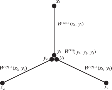
Figure 1: The diagram of the bi-spectrum

Next, we calculate the non-Gaussian spectrums of the primordial curvature perturbation $\zeta(\hbox{\boldmath{$x$}})$. The bi-spectrum for $\zeta(\hbox{\boldmath{$x$}})$ is expressed by the cubic interaction $W^{(3)}(\hbox{\boldmath{$x$}}_{1},\,\hbox{\boldmath{$x$}}_{2},\,\hbox{\boldmath{$x$}}_{3})$ as

$$\langle\zeta(\hbox{\boldmath{$x$}}_{1})\zeta(\hbox{\boldmath{$x$}}_{2})\zeta(\hbox{\boldmath{$x$}}_{3})\rangle_{\rm conn}=-\int\prod_{i=1}^{3}{\rm d}^{3}\hbox{\boldmath{$y$}}_{i}\,W^{(2)\,-1}(\hbox{\boldmath{$x$}}_{i}\,,\hbox{\boldmath{$y$}}_{i})\,W^{(3)}(\hbox{\boldmath{$y$}}_{1},\,\hbox{\boldmath{$y$}}_{2},\,\hbox{\boldmath{$y$}}_{3})\,,$$ (65)

where using Eqs. (20) and (48), we obtain

$$W^{(3)}(\hbox{\boldmath{$x$}}_{1},\,\hbox{\boldmath{$x$}}_{2},\,\hbox{\boldmath{$x$}}_{3})=-2\,{\rm Re}\Bigl{[}(\lambda u)^{3}\langle O(\hbox{\boldmath{$x$}}_{1})O(\hbox{\boldmath{$x$}}_{2})O(\hbox{\boldmath{$x$}}_{3})\rangle_{u}$$ (66)

$$\qquad\qquad\qquad\qquad\qquad\qquad-\lambda^{3}u^{2}\{\delta(\hbox{\boldmath{$x$}}_{1}-\hbox{\boldmath{$x$}}_{2})\langle O(\hbox{\boldmath{$x$}}_{2})O(\hbox{\boldmath{$x$}}_{3})\rangle_{u}+({\rm 2\,{\rm cyclic~{}perms}})\}\Bigr{]}\,.$$ (67)

In Eq. (65), we noted that $W^{(3)}(\hbox{\boldmath{$x$}}_{1},\,\hbox{\boldmath{$x$}}_{2},\,\hbox{\boldmath{$x$}}_{3})$ is symmetric under an exchange of the arguments $\hbox{\boldmath{$x$}}_{1}$, $\hbox{\boldmath{$x$}}_{2}$, and $\hbox{\boldmath{$x$}}_{3}$. The expression of Eq. (65) can be diagrammatically understood as in Fig. 1. Performing the Fourier transformation, the bi-spectrum for $\zeta(\hbox{\boldmath{$k$}})$ is given by

$$\langle\zeta(\hbox{\boldmath{$k$}}_{1})\zeta(\hbox{\boldmath{$k$}}_{2})\zeta(\hbox{\boldmath{$k$}}_{3})\rangle_{\rm conn} =(2\pi)^{3}\delta(\hbox{\boldmath{$k$}}_{1}+\hbox{\boldmath{$k$}}_{2}+\hbox{\boldmath{$k$}}_{3})\,B\left(\hbox{\boldmath{$k$}}_{1},\,\hbox{\boldmath{$k$}}_{2},\,\hbox{\boldmath{$k$}}_{3}\right)\,$$ (69)

with

$$B\left(\hbox{\boldmath{$k$}}_{1},\,\hbox{\boldmath{$k$}}_{2},\,\hbox{\boldmath{$k$}}_{3}\right)=-\frac{\hat{W}^{(3)}\left(\hbox{\boldmath{$k$}}_{1},\,\hbox{\boldmath{$k$}}_{2},\,\hbox{\boldmath{$k$}}_{3}\right)}{\hat{W}^{(2)}(k_{1})\hat{W}^{(2)}(k_{2})\hat{W}^{(2)}(k_{3})}=-\hat{W}^{(3)}\left(\hbox{\boldmath{$k$}}_{1},\,\hbox{\boldmath{$k$}}_{2},\,\hbox{\boldmath{$k$}}_{3}\right)\prod_{i=1}^{3}P(k_{i})\,,$$ (70)

where $\hat{W}^{(3)}\left(\hbox{\boldmath{$k$}}_{1},\,\hbox{\boldmath{$k$}}_{2},\,\hbox{\boldmath{$k$}}_{3}\right)$ is defined as

$$(2\pi)^{3}\delta(\hbox{\boldmath{$k$}}_{1}+\hbox{\boldmath{$k$}}_{2}+\hbox{\boldmath{$k$}}_{3})\hat{W}^{(3)}\left(\hbox{\boldmath{$k$}}_{1},\,\hbox{\boldmath{$k$}}_{2},\,\hbox{\boldmath{$k$}}_{3}\right)\equiv\prod_{i=1}^{3}\int{\rm d}^{3}\hbox{\boldmath{$x$}}_{i}\,e^{-i\hbox{\boldmath{\scriptsize$k$}}_{i}\cdot\hbox{\boldmath{\scriptsize$x$}}_{i}}W^{(3)}(\hbox{\boldmath{$x$}}_{1},\,\hbox{\boldmath{$x$}}_{2},\,\hbox{\boldmath{$x$}}_{3})\,.$$ (71)

The bi-spectrum (69) agrees with the one obtained in Ref. [18] by using the holographic renormalization group method.

4.3 The tri-spectrum

Next, we calculate the tri-spectrum of $\zeta(\hbox{\boldmath{$x$}})$. As is depicted in Fig. 2, the tri-spectrum is composed of the two-different diagrams and is given by

$$\langle\zeta(\hbox{\boldmath{$x$}}_{1})\zeta(\hbox{\boldmath{$x$}}_{2})\zeta(\hbox{\boldmath{$x$}}_{3})\zeta(\hbox{\boldmath{$x$}}_{4})\rangle_{\rm conn}$$ (72)

$$=-\int\prod_{i=1}^{4}{\rm d}^{3}\hbox{\boldmath{$y$}}_{i}\,W^{(2)\,-1}(\hbox{\boldmath{$x$}}_{i}\,,\hbox{\boldmath{$y$}}_{i})\,W^{(4)}(\hbox{\boldmath{$y$}}_{1},\,\hbox{\boldmath{$y$}}_{2},\,\hbox{\boldmath{$y$}}_{3},\,\hbox{\boldmath{$y$}}_{4})$$ (73)

$$\qquad+\int\prod_{i=1}^{3}{\rm d}^{3}\hbox{\boldmath{$y$}}_{i}\int{\rm d}^{3}\hbox{\boldmath{$z$}}_{i}\,W^{(2)\,-1}(\hbox{\boldmath{$x$}}_{1},\,\hbox{\boldmath{$y$}}_{1})W^{(2)\,-1}(\hbox{\boldmath{$x$}}_{2},\,\hbox{\boldmath{$y$}}_{2})$$ (74)

$$\qquad\qquad\times W^{(2)\,-1}(\hbox{\boldmath{$x$}}_{3},\,\hbox{\boldmath{$z$}}_{1})W^{(2)\,-1}(\hbox{\boldmath{$x$}}_{4},\,\hbox{\boldmath{$z$}}_{2})W^{(2)\,-1}(\hbox{\boldmath{$y$}}_{3},\,\hbox{\boldmath{$z$}}_{3})W^{(3)}(\hbox{\boldmath{$y$}}_{1},\,\hbox{\boldmath{$y$}}_{2},\,\hbox{\boldmath{$y$}}_{3})W^{(3)}(\hbox{\boldmath{$z$}}_{1},\,\hbox{\boldmath{$z$}}_{2},\,\hbox{\boldmath{$z$}}_{3})$$ (75)

$$\qquad+(\hbox{\boldmath{$x$}}_{2}\leftrightarrow\hbox{\boldmath{$x$}}_{3})+(\hbox{\boldmath{$x$}}_{2}\leftrightarrow\hbox{\boldmath{$x$}}_{4})\,,$$ (76)

where the first term stems from the diagram in the left panel of Fig. 2 and the second term stems from the diagram in the right.

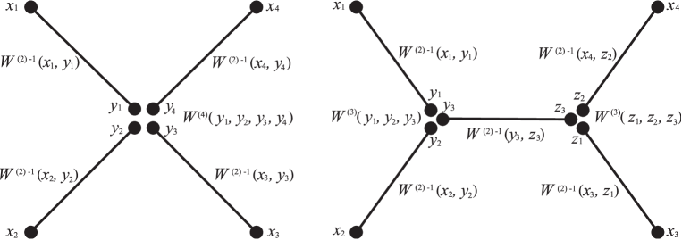
Figure 2: The diagrams of the tri-spectrum

The terms in the last lines are the contributions from the diagram with the vertex $\hbox{\boldmath{$x$}}_{2}$ in the right panel of Fig. 2 exchanged with $\hbox{\boldmath{$x$}}_{3}$ and $\hbox{\boldmath{$x$}}_{4}$, respectively. Here, noticing the fact that $W^{(3)}(\hbox{\boldmath{$x$}}_{1},\,\hbox{\boldmath{$x$}}_{2},\,\hbox{\boldmath{$x$}}_{3})$ and $W^{(4)}(\hbox{\boldmath{$x$}}_{1},\,\hbox{\boldmath{$x$}}_{2},\,\hbox{\boldmath{$x$}}_{3},\,\hbox{\boldmath{$x$}}_{4})$ are symmetric under an exchange of their arguments, we summed up the terms which give the same contribution. Equations  (20) and (48) yield

$$W^{(4)}(\hbox{\boldmath{$x$}}_{1},\,\hbox{\boldmath{$x$}}_{2},\,\hbox{\boldmath{$x$}}_{3},\,\hbox{\boldmath{$x$}}_{4})$$ (77)

$$=-2\,{\rm Re}\biggl{[}(\lambda u)^{4}\langle O(\hbox{\boldmath{$x$}}_{1})\cdots O(\hbox{\boldmath{$x$}}_{4})\rangle_{u}-\lambda^{4}u^{3}\!\left\{\delta(\hbox{\boldmath{$x$}}_{1}-\hbox{\boldmath{$x$}}_{2})\langle O(\hbox{\boldmath{$x$}}_{2})O(\hbox{\boldmath{$x$}}_{3})O(\hbox{\boldmath{$x$}}_{4})\rangle_{u}+\left(5\,\,{\rm cyclic~{}perms}\right)\!\right\}$$ (78)

$$\qquad\qquad\quad+\lambda^{4}u^{2}\{\delta(\hbox{\boldmath{$x$}}_{1}-\hbox{\boldmath{$x$}}_{2})\delta(\hbox{\boldmath{$x$}}_{2}-\hbox{\boldmath{$x$}}_{3})\langle O(\hbox{\boldmath{$x$}}_{3})O(\hbox{\boldmath{$x$}}_{4})\rangle_{u}+(3\,\,{\rm{\rm cyclic~{}perms}})\}\biggr{]}\,.$$ (79)

In the Fourier space, the tri-spectrum is given by

$$\langle\zeta(\hbox{\boldmath{$k$}}_{1})\zeta(\hbox{\boldmath{$k$}}_{2})\zeta(\hbox{\boldmath{$k$}}_{3})\zeta(\hbox{\boldmath{$k$}}_{4})\rangle_{\rm conn} =(2\pi)^{3}\,\delta\left(\sum_{i=1}^{4}\hbox{\boldmath{$k$}}_{i}\right)\,T\left(\hbox{\boldmath{$k$}}_{1},\,\hbox{\boldmath{$k$}}_{2},\,\hbox{\boldmath{$k$}}_{3},\,\hbox{\boldmath{$k$}}_{4}\right)\,,$$ (80)

with

$$T(\hbox{\boldmath{$k$}}_{1},\,\hbox{\boldmath{$k$}}_{2},\,\hbox{\boldmath{$k$}}_{3},\,\hbox{\boldmath{$k$}}_{4})=T_{1}\left(\hbox{\boldmath{$k$}}_{1},\,\hbox{\boldmath{$k$}}_{2},\,\hbox{\boldmath{$k$}}_{3},\,\hbox{\boldmath{$k$}}_{4}\right)+T_{2}\left(\hbox{\boldmath{$k$}}_{1},\,\hbox{\boldmath{$k$}}_{2},\,\hbox{\boldmath{$k$}}_{3},\,\hbox{\boldmath{$k$}}_{4}\right)$$ (81)

$$\qquad\qquad\qquad\qquad\qquad\qquad+T_{2}\left(\hbox{\boldmath{$k$}}_{1},\,\hbox{\boldmath{$k$}}_{3},\,\hbox{\boldmath{$k$}}_{2},\,\hbox{\boldmath{$k$}}_{4}\right)+T_{2}\left(\hbox{\boldmath{$k$}}_{1},\,\hbox{\boldmath{$k$}}_{4},\,\hbox{\boldmath{$k$}}_{3},\,\hbox{\boldmath{$k$}}_{1}\right)\,,$$ (82)

$$T_{1}(\hbox{\boldmath{$k$}}_{1},\,\hbox{\boldmath{$k$}}_{2},\,\hbox{\boldmath{$k$}}_{3},\,\hbox{\boldmath{$k$}}_{4})=-\hat{W}^{(4)}\left(\hbox{\boldmath{$k$}}_{1},\,\hbox{\boldmath{$k$}}_{2},\,\hbox{\boldmath{$k$}}_{3},\,\hbox{\boldmath{$k$}}_{4}\right)\prod_{i=1}^{4}P(k_{i})\,,$$ (83)

$$T_{2}(\hbox{\boldmath{$k$}}_{1},\,\hbox{\boldmath{$k$}}_{2},\,\hbox{\boldmath{$k$}}_{3},\,\hbox{\boldmath{$k$}}_{4})=\hat{W}^{(3)}\left(\hbox{\boldmath{$k$}}_{1},\,\hbox{\boldmath{$k$}}_{2},\,-\hbox{\boldmath{$k$}}_{12}\right)\hat{W}^{(3)}\left(\hbox{\boldmath{$k$}}_{3},\,\hbox{\boldmath{$k$}}_{4},\,-\hbox{\boldmath{$k$}}_{34}\right)P(k_{12})\prod_{i=1}^{4}P(k_{i})\,,$$ (84)

where we introduced the Fourier mode of $W^{(4)}$ as

$$(2\pi)^{3}\hat{W}^{(4)}\left(\hbox{\boldmath{$k$}}_{1},\,\hbox{\boldmath{$k$}}_{2},\,\hbox{\boldmath{$k$}}_{3},\,\hbox{\boldmath{$k$}}_{4}\right)\delta\left(\sum_{i=1}^{4}\hbox{\boldmath{$k$}}_{i}\right)\equiv\prod_{i=1}^{4}\int{\rm d}^{3}\hbox{\boldmath{$x$}}_{i}\,e^{-i\hbox{\boldmath{\scriptsize$k$}}_{i}\cdot\hbox{\boldmath{\scriptsize$x$}}_{i}}W^{(4)}(\hbox{\boldmath{$x$}}_{1},\,\hbox{\boldmath{$x$}}_{2},\,\hbox{\boldmath{$x$}}_{3},\,\hbox{\boldmath{$x$}}_{4})\,,$$ (85)

and the momentum $\hbox{\boldmath{$k$}}_{ij}$ and its absolute value as $\hbox{\boldmath{$k$}}_{ij}\equiv\hbox{\boldmath{$k$}}_{i}+\hbox{\boldmath{$k$}}_{j}$ and $k_{ij}\equiv|\hbox{\boldmath{$k$}}_{ij}|$. Note that using the bi-spectrum $B(\hbox{\boldmath{$k$}}_{1},\,\hbox{\boldmath{$k$}}_{2},\,\hbox{\boldmath{$k$}}_{3})$, we can express $T_{2}(\hbox{\boldmath{$k$}}_{1},\,\hbox{\boldmath{$k$}}_{2},\,\hbox{\boldmath{$k$}}_{3},\,\hbox{\boldmath{$k$}}_{4})$ as

$$T_{2}(\hbox{\boldmath{$k$}}_{1},\,\hbox{\boldmath{$k$}}_{2},\,\hbox{\boldmath{$k$}}_{3},\,\hbox{\boldmath{$k$}}_{4})=\frac{B\left(\hbox{\boldmath{$k$}}_{1},\,\hbox{\boldmath{$k$}}_{2},\,-\hbox{\boldmath{$k$}}_{12}\right)B\left(\hbox{\boldmath{$k$}}_{3},\,\hbox{\boldmath{$k$}}_{4},\,-\hbox{\boldmath{$k$}}_{34}\right)}{P(k_{12})}\,.$$ (86)

An extension to higher-point correlators proceeds in a straightforward manner. Thus, once we obtain all the $m$-point functions for the QFT operator $O(\hbox{\boldmath{$x$}})$ with $m\leq n$, we can easily obtain the $n$-point functions for the curvature perturbation $\zeta(\hbox{\boldmath{$x$}})$. Note that although the computation of the $n$-point functions proceeds as in the perturbative expansion of the weakly coupled QFT, the propagator $W^{(2)\,-1}(\hbox{\boldmath{$x$}}_{1},\,\hbox{\boldmath{$x$}}_{2})$ and the vertex functions $W^{(n)}(\hbox{\boldmath{$x$}}_{1},\,\cdots,\,\hbox{\boldmath{$x$}}_{n})$ with $n\geq 3$ can include the resumed non-perturbative effect of the boundary QFT.

4.4 The Suyama-Yamaguchi inequality

In the conventional inflation, where the gravity is weakly coupled and the perturbative analysis in the bulk is valid, the non-linear parameters $f_{\rm NL}$ and $\tau_{\rm NL}$:

$$f_{\rm NL}\equiv\frac{5}{12}\lim_{k_{1}\to 0}\frac{B(\hbox{\boldmath{$k$}}_{1},\,\hbox{\boldmath{$k$}}_{2},\,-(\hbox{\boldmath{$k$}}_{1}+\hbox{\boldmath{$k$}}_{2}))}{P(k_{1})P(k_{2})}$$ (87)

$$\tau_{\rm NL}\equiv\frac{1}{4}\lim_{k_{12}\to 0}\frac{T(\hbox{\boldmath{$k$}}_{1},\,\hbox{\boldmath{$k$}}_{2},\,\hbox{\boldmath{$k$}}_{3},\,\hbox{\boldmath{$k$}}_{4})}{P(k_{1})P(k_{3})P(k_{12})}$$ (88)

are known to satisfy the so-called Suyama-Yamaguchi (SY) inequality [38]:

$$\tau_{\rm NL}\geq\left(\frac{6}{5}f_{\rm NL}\right)^{2}\,.$$ (89)

The SY inequality is first shown by using the $\delta N$ formalism, which gives a map between the field fluctuation at the Hubble crossing time and the fluctuation of the number of $e$-folding that approximately agrees with the curvature perturbation at the end of inflation, under the assumption that the field fluctuation is totally Gaussian at the Hubble crossing time. Under this assumption, the equality holds for a single field model of inflation. A generalization of the SY inequality has been intended later, for instance in Refs. [39, 40]. The authors of Ref. [40] showed that if $\tau_{\rm NL}$ and $(f_{\rm NL})^{2}$ are either momentum independent or have the same momentum dependence, we can verify the SY inequality as well as in the presence of the non-Gaussianity at the Hubble crossing time.

Here, we study the validity of this inequality in holographic inflation. As the limit $k_{12}\to 0$, more precisely, we mean the limit $k_{12}\ll k_{1},k_{3},k_{13}$. Using Eq. (86), we obtain the contribution of the second term in Eq. (82) to $\tau_{\rm NL}$ as

$$\lim_{k_{12}\to 0}\frac{T_{2}(\hbox{\boldmath{$k$}}_{1},\,\hbox{\boldmath{$k$}}_{2},\,\hbox{\boldmath{$k$}}_{3},\,\hbox{\boldmath{$k$}}_{4})}{P(k_{1})P(k_{3})P(k_{12})}\to 4\left(\frac{6}{5}f_{\rm NL}\right)^{2}\,.$$ (90)

The third term in Eq. (82) gives

$$\frac{T_{2}(\hbox{\boldmath{$k$}}_{1},\,\hbox{\boldmath{$k$}}_{3},\,\hbox{\boldmath{$k$}}_{2},\,\hbox{\boldmath{$k$}}_{4})}{P(k_{1})P(k_{3})P(k_{12})}=\frac{P(k_{13})}{P(k_{12})}\left\{\frac{B(\hbox{\boldmath{$k$}}_{1},\,-\hbox{\boldmath{$k$}}_{13},\,\hbox{\boldmath{$k$}}_{3})}{P(k_{1})P(k_{13})}\right\}^{2}\,,$$ (91)

where we noted that $\hbox{\boldmath{$k$}}_{1}\simeq-\hbox{\boldmath{$k$}}_{2}$ and $\hbox{\boldmath{$k$}}_{3}\simeq-\hbox{\boldmath{$k$}}_{4}$ in the limit $k_{12}\to 0$. The term in the curly brackets is expressed by $k_{1}/k_{3}$ or $k_{3}/k_{1}$ which are larger than $k_{12}/k_{1}$ and $k_{12}/k_{3}$. Therefore the right hand side of Eq. (91) with $1/P(k_{12})$, which approaches 0 in the limit $k_{12}\to 0$, vanishes. The fourth term in Eq. (82) also vanishes in this limit. Thus, we obtain

$$\tau_{\rm NL}-\left(\frac{6}{5}f_{\rm NL}\right)^{2}=-\frac{1}{4}\lim_{k_{12}\to 0}\hat{W}^{(4)}\left(\hbox{\boldmath{$k$}}_{1},\,\hbox{\boldmath{$k$}}_{2},\,\hbox{\boldmath{$k$}}_{3},\,\hbox{\boldmath{$k$}}_{4}\right)\frac{P(k_{1})P(k_{3})}{P(k_{12})}\,,$$ (92)

and hence the SY inequality holds, if the right hand side of Eq. (92) is equal to or is larger than $0$. If the vertex function $\hat{W}^{(4)}(\hbox{\boldmath{$k$}}_{1},\,\hbox{\boldmath{$k$}}_{2},\,\hbox{\boldmath{$k$}}_{3},\,\hbox{\boldmath{$k$}}_{4})$ does not yield a singular pole in the limit $k_{12}\to 0$, the right hand side of Eq. (92) vanishes and hence the equality holds as in single field models of the weakly coupled inflation. However, the momentum dependence of the vertex function $\hat{W}^{(4)}$ which includes the non-perturbative effect, is rather less obvious. To capture the momentum dependence of the vertex function $\hat{W}^{(4)}$, we need to specify the four-point function of $O(\hbox{\boldmath{$x$}})$. As is known, even in CFT, the higher point functions $\langle O(\hbox{\boldmath{$x$}}_{1})\cdots O(\hbox{\boldmath{$x$}}_{n})\rangle_{u=0}$ with $n\geq 4$ are not determined only by the conformal symmetry. Actually, the Ward-Takahashi identities leave functional degree of freedom in the four point function [36]. It would be interesting to examine the validity of the SY inequality in a particular model of the holographic inflation.

5 Concluding remarks

In this paper, using the holographic formula (15) and the Ward-Takahashi identity, we provided the relation between the $n$-point functions of the bulk gravitational field $\zeta$ and $n$-point functions of the QFT operator $O$ on the boundary. In contrast with Refs. [18, 27], we expressed the Ward-Takahashi identity so that it directly relates the generating functional $Z_{\rm QFT}$ to the $n$-point functions of the QFT operator $O$. This bypasses a redundant step which refers to the energy-momentum tensor, making the computation more compact and transparent. This result can be also used to compute the spectra of $\zeta$ based on the domain wall/cosmology correspondence, which is addressed in Refs. [13, 14, 15, 16, 17, 18]. In these papers, the description of the spectra is provided based on the holographic renormalization method. We showed that both methods lead to the same formula relating the $n$-point functions of $\zeta$ and those of $O$. In Refs. [13, 14, 17], the correlators of the tensor modes are also studied. An extension of our argument to include these correlators is left for a future study. We also studied the validity of the Suyama-Yamaguchi inequality and showed that unless $W^{(4)}$ yields a singular pole in the limit $k_{12}\to 0$, $\tau_{\rm NL}$ agrees with $(6f_{\rm NL}/5)^{2}$ as has been known in weakly coupled single field models.

When we calculate the $n$-point functions of the curvature perturbation $\zeta$, using the vertex functions $W^{(n)}(\hbox{\boldmath{$x$}}_{1},\cdots,\,\hbox{\boldmath{$x$}}_{n})$, we neglected the loop corrections. (Note that the vertex function $W^{(n)}(\hbox{\boldmath{$x$}}_{1},\cdots,\,\hbox{\boldmath{$x$}}_{n})$ includes the non-perturbative effect of the QFT on the boundary.) As a final issue of the present article, we examine the validity of this approximation. Loop diagrams can be obtained by inserting additional interaction vertices to the tree level diagrams, presented in Figs. 1 and 2. A naive order estimation tells that inserting a further $n$-point interaction vertex

$$\prod_{i=1}^{n}\int{\rm d}^{3}\hbox{\boldmath{$x$}}_{i}\zeta(\hbox{\boldmath{$x$}}_{i})W^{(n)}(\hbox{\boldmath{$x$}}_{1},\,\cdots,\,\hbox{\boldmath{$x$}}_{n})$$

changes the amplitude by

$$|W^{(n)}\zeta^{n}|={\cal O}(\lambda^{n}u^{m})\times{\cal O}\left((\lambda uc^{1/2})^{-n}\right)={\cal O}(u^{m-n}c^{-n/2})\,,$$

with $1\leq m\leq n$. Here, we noted that as is suggested by the order of the propagator given in Eq. (61), the amplitude of $\zeta$ amounts to $1/(\lambda uc^{1/2})$ and the contribution of the $n$-th vertex function amounts to $\lambda^{n}u^{m}$. Therefore, to keep the loop corrections sub dominant, the central charge should be $c\gg 1$. Since the central charge is supposed to be the number of degrees of freedom, this condition can be thought of as the condition of the so-called large $N$ approximation. When we use Eq. (62), $c\gg 1$ yields $(H/M_{\rm pl})\ll 1$, which requests that inflation should take place in the sub-Planck energy scale. Note that the energy scale of inflation, $H$, can exceed the string scale, admitting the stringy corrections.

References

• [1] P. A. R. Ade et al. [ Planck Collaboration], arXiv:1303.5082 [astro-ph.CO].
• [2] J. M. Maldacena, Adv. Theor. Math. Phys.  2, 231 (1998) [hep-th/9711200].
• [3] S. S. Gubser, I. R. Klebanov and A. M. Polyakov, Phys. Lett. B 428, 105 (1998) [hep-th/9802109].
• [4] E. Witten, Adv. Theor. Math. Phys.  2, 253 (1998) [hep-th/9802150].
• [5] A. Strominger, JHEP 0110, 034 (2001) [hep-th/0106113].
• [6] A. Strominger, JHEP 0111, 049 (2001) [hep-th/0110087].
• [7] E. Witten, hep-th/0106109.
• [8] R. Bousso, A. Maloney and A. Strominger, Phys. Rev. D 65, 104039 (2002) [hep-th/0112218].
• [9] D. Harlow and D. Stanford, arXiv:1104.2621 [hep-th].
• [10] D. Anninos, T. Hartman and A. Strominger, arXiv:1108.5735 [hep-th].
• [11] J. M. Maldacena, JHEP 0305, 013 (2003) [astro-ph/0210603].
• [12] D. Seery and J. E. Lidsey, JCAP 0606, 001 (2006) [astro-ph/0604209].
• [13] P. McFadden and K. Skenderis, Phys. Rev.  D 81, 021301 (2010) [arXiv:0907.5542 [hep-th]].
• [14] P. McFadden, K. Skenderis, J. Phys. Conf. Ser.  222, 012007 (2010). [arXiv:1001.2007 [hep-th]].
• [15] P. McFadden, K. Skenderis, [arXiv:1010.0244 [hep-th]].
• [16] P. McFadden, K. Skenderis, JCAP 1105, 013 (2011). [arXiv:1011.0452 [hep-th]].
• [17] P. McFadden and K. Skenderis, JCAP 1106, 030 (2011) [arXiv:1104.3894 [hep-th]].
• [18] A. Bzowski, P. McFadden and K. Skenderis, arXiv:1211.4550 [hep-th].
• [19] K. Skenderis and P. K. Townsend, Phys. Rev. Lett.  96, 191301 (2006) [arXiv:hep-th/0602260].
• [20] K. Skenderis and P. K. Townsend, J. Phys. A 40, 6733 (2007) [arXiv:hep-th/0610253].
• [21] J. de Boer, E. P. Verlinde and H. L. Verlinde, JHEP 0008, 003 (2000) [hep-th/9912012].
• [22] M. Bianchi, D. Z. Freedman and K. Skenderis, Nucl. Phys. B 631, 159 (2002) [hep-th/0112119].
• [23] K. Skenderis, Class. Quant. Grav.  19, 5849 (2002) [hep-th/0209067].
• [24] R. Easther, R. Flauger, P. McFadden and K. Skenderis, arXiv:1104.2040 [astro-ph.CO].
• [25] M. Dias, Phys. Rev.  D 84, 023512 (2011) [arXiv:1104.0625 [astro-ph.CO]].
• [26] J. P. van der Schaar, JHEP 0401, 070 (2004) [hep-th/0307271].
• [27] K. Schalm, G. Shiu and T. van der Aalst, arXiv:1211.2157 [hep-th].
• [28] I. Mata, S. Raju and S. Trivedi, arXiv:1211.5482 [hep-th].
• [29] J. Garriga and A. Vilenkin, JCAP 0911, 020 (2009) [arXiv:0905.1509 [hep-th]].
• [30] D. Harlow and L. Susskind, arXiv:1012.5302 [hep-th].
• [31] T. J. Hollowood, arXiv:0909.0859 [hep-th].
• [32] I. R. Klebanov, S. S. Pufu and B. R. Safdi, JHEP 1110, 038 (2011) [arXiv:1105.4598 [hep-th]].
• [33] K. Fujikawa, Phys. Rev. D 23, 2262 (1981).
• [34] N. D. Birrell and P. C. W. Davies, Quantum fields in curved space, Cambridge (1982)
• [35] P. Di Francesco, P. Mathieu and D. S$\acute{\rm e}$n$\acute{\rm e}$chal, Conformal Field Theory, Springer Verlag, 1996
• [36] I. Antoniadis, P. O. Mazur and E. Mottola, JCAP 1209, 024 (2012) [arXiv:1103.4164 [gr-qc]].
• [37] Y. Nakayama, arXiv:1302.0884 [hep-th].
• [38] T. Suyama and M. Yamaguchi, Phys. Rev. D 77, 023505 (2008) [arXiv:0709.2545 [astro-ph]].
• [39] A. Kehagias and A. Riotto, Nucl. Phys. B 864, 492 (2012) [arXiv:1205.1523 [hep-th]].
• [40] V. Assassi, D. Baumann and D. Green, JCAP 1211, 047 (2012) [arXiv:1204.4207 [hep-th]].