A Numerical Approach to
Scalar Nonlocal Conservation Laws

Abstract

We address the study of a class of 1D nonlocal conservation laws from a numerical point of view. First, we present an algorithm to numerically integrate them and prove its convergence. Then, we use this algorithm to investigate various analytical properties, obtaining evidence that usual properties of standard conservation laws fail in the nonlocal setting. Moreover, on the basis of our numerical integrations, we are lead to conjecture the convergence of the nonlocal equation to the local ones, although no analytical results are, to our knowledge, available in this context.

2000 Mathematics Subject Classification: 35L65

Keywords: Nonlocal Conservation Laws; Lax Friedrichs Scheme.

1 Introduction

Conservation laws with nonlocal fluxes have appeared recently in the literature, arising naturally in many fields of application, such as in crowd dynamics (see [3, 4, 5, 15] and the references therein), or in models inspired from biology, see [2, 8, 9, 10].

In this paper, we initiate the study of these equations from a numerical point of view. First, we prove the convergence of a finite volume algorithm to numerically integrate a class of one-dimensional conservation laws with a nonlocal flow. Then, we use this algorithm to show peculiar properties of these nonlocal equations and, in particular, how they differ from the usual local ones.

Consider the scalar equation

$$\left\{\begin{array}[]{l}\partial_{t}\rho+\partial_{x}\left(f(t,x,\rho)\,v(\rho*\eta)\right)=0\\ \rho(0,x)=\rho^{o}(x)\end{array}\right.\qquad(t,x)\in{\mathbb{R}}^{+}\times{\mathbb{R}}$$ (1.1)

which slightly extends, in the 1D case, the class of equations considered in [4, 5]. We present below a numerical scheme to integrate (1.1) and prove its convergence. As a byproduct, we also establish an existence result for (1.1), thus slightly extending [4, Theorem 2.2] in the 1D case.

This numerical algorithm is then implemented and used to investigate various properties of (1.1). First, we provide evidence that the usual Maximum Principle for scalar conservation laws fails in the case of (1.1). Another integration shows that the total variation of the solution to (1.1) may well sharply increase, contrary to what happens in the standard local situation. Remark that both these examples are in agreement with the estimates we rigorously obtain on the approximate solutions.

Of particular interest is the limit $\eta\to\delta$, $\delta$ being the Dirac measure centered at the origin. Numerical integrations show that the solutions to (1.1) converge to that of

$$\left\{\begin{array}[]{l}\partial_{t}\rho+\partial_{x}\left(f(t,x,\rho)\,v(\rho)\right)=0\\ \rho(0,x)=\rho^{o}(x)\end{array}\right.\qquad(t,x)\in{\mathbb{R}}^{+}\times{\mathbb{R}}$$ (1.2)

although no rigorous proof of this convergence is, to our knowledge, known. Remark that in the nonlocal case, well posedness results are available also in the case of systems in several space dimensions, see [5, 6]. Hence, the ability of passing to the limit $\eta\to\delta$ might help in the search for analytical results about systems of conservation laws in several space dimensions.

Let us make the following remarks. First, the scheme presented below has an associated CFL condition. The CFL condition is often interpreted through a comparison between the numerical propagation speed and the analytical one, see for instance [13, § 4.4, p. 68]. In the present nonlocal case (1.1), information propagates at an infinite speed, due to the presence of the term $\eta*\rho$. Nevertheless, also in the nonlocal case (1.1) a suitable CFL condition plays a key role, see (2.8).

Second, the scheme presented below is not monotone in the sense of the usual definition [13, Formula (12.42)], as follows from the integration in Section 3.2. There, both constant initial data $\bar{\rho}=0$ and $\bar{\rho}=1$ yield constant solutions, but the initial datum (3.5), although it attains values in $[0,1]$, yields a solution exceeding $1$. Nevertheless, the scheme (2.10) enjoys several properties of monotone schemes, proved in the lemmas in Section 2.

Remark 1.1.

Throughout this work, we follow the usual habit of referring to (1.1) as to a nonlocal equation and, hence, to the standard case (1.2) as to the local case. However, whenever the support of $\eta$ is bounded, it might seem more appropriate to call (1.1) a local equation and (1.2) the punctual case.

The next section deals with the definition of the algorithm and with the statement of the estimates which ensure its convergence, as well as the entropicity of the limit solution. Section 3 deals with various numerical integrations of (1.1). All proofs are deferred to the last Section 4.

2 Main Results

Throughout, we set ${\mathbb{R}}^{+}=\left[0,+\infty\right[$.

As a starting point, we state what we mean by solution to (1.1), see also [4, Definition 2.1].

Definition 2.1.

Let $T>0$. Fix $\rho^{o}\in{\mathbf{L}^{\infty}}({\mathbb{R}};{\mathbb{R}})$. A weak entropy solution to (1.1) on $[0,T]$ is a bounded measurable Kružkov solution $\rho\in\mathbf{C}^{0}\left([0,T];{\mathbf{L}_{loc}^{1}}({\mathbb{R}};{\mathbb{R}})\right)$ to

$$\left\{\begin{array}[]{@{\,}l@{}}\partial_{t}\rho+\partial_{x}\left(f(t,x,\rho)\,V(t,x)\right)=0\\ \rho(0,x)=\rho^{o}(x)\end{array}\right.\quad\mbox{ where}\quad V(t,x)=v\!\left((\rho(t)*\eta)(x)\right)\,.$$

For the definition of Kružkov solution, see for instance [7, Paragraph 6.2] or [12, Definition 1]. Here, as usual,

$$\left(\rho(t)*\eta\right)(x)=\int_{{\mathbb{R}}}\rho(t,\xi)\;\eta(x-\xi)\,\mathinner{\mathrm{d}{\xi}}\,.$$

Remark that the assumptions

$$f\in\mathbf{C}^{2}({\mathbb{R}}^{+}\times{\mathbb{R}}\times{\mathbb{R}};{\mathbb{R}}) \left\{\begin{array}[]{rcl}\displaystyle\sup_{t,x,\rho}{\left|\partial_{\rho}f(t,x,\rho)\right|}&<&+\infty\\ \displaystyle\sup_{t,x}{\left|\partial_{x}f(t,x,\rho)\right|}&<&C\,{\left|\rho\right|}\\ \displaystyle\sup_{t,x}{\left|\partial^{2}_{xx}f(t,x,\rho)\right|}&<&C\,{\left|\rho\right|}\\ \displaystyle\forall\,t,x\quad f(t,x,0)&=&0\end{array}\right.$$ and (2.5)

$$v\in(\mathbf{C}^{2}\cap{\mathbf{W}^{1,\infty}})({\mathbb{R}};{\mathbb{R}}) \qquad\eta\in(\mathbf{C}^{2}\cap{\mathbf{W}^{2,\infty}})({\mathbb{R}};{\mathbb{R}})$$ and (2.6)

ensure that the transport equation in Definition 2.1 fits in Kružkov framework, see [7, 12]. From the modeling point of view, it is natural to require that the kernel $\eta$ attains only positive (or non-negative) values. However, this requirement is not necessary for the analytical results below.

Below, Remark 2.3 and Lemma 2.5 provide uniform ${\mathbf{L}^{\infty}}$ bounds on the solution to (1.1) under conditions (2.5)–(2.6) on the equations and for data in ${\mathbf{L}^{\infty}}$. Therefore, the apparently strong requirement ${\left\|\partial_{\rho}f\right\|}_{{\mathbf{L}^{\infty}}}<+\infty$ can be easily relaxed to

$$\sup_{t\in{\mathbb{R}}^{+},\,x\in{\mathbb{R}},\,\rho\in[-M,M]}{\left|\partial_{\rho}f(t,x,\rho)\right|}<+\infty$$

for a suitable positive $M$. Moreover, the usual sublinearity condition $\sup_{t,x}{\left|\partial_{x}f(t,x,\rho)\right|}<C(1+{\left|\rho\right|})$ takes the form $\sup_{t,x}{\left|\partial_{x}f(t,x,\rho)\right|}<C{\left|\rho\right|}$ in (2.5) due to the assumption $f(t,x,0)=0$ for all $t$ and $x$.

Introduce a uniform mesh with size $h$ along the $x$ axis and size $\tau$ along the $t$ axis. Throughout, we assume that

$$h<1/C$$ (2.7)

with $C$ as in (2.5) and that the following CFL condition is satisfied:

$$\lambda\,\left(1+2\,{\left\|\partial_{\rho}f\right\|}_{{\mathbf{L}^{\infty}}}\right){\left\|v\right\|}_{{\mathbf{L}^{\infty}}}\leq\frac{1}{6}$$ (2.8)

where, as usual, $\lambda=\tau/h$.

Consider the following Lax–Friedrichs type scheme:

$$\left\{\begin{array}[]{lcl}\rho^{n+1}_{j}&=&\rho^{n}_{j}-\lambda\left(\mathbf{f}^{n}_{j+1/2}(\rho^{n}_{j},\rho^{n}_{j+1})-\mathbf{f}^{n}_{j-1/2}(\rho^{n}_{j-1},\rho^{n}_{j})\right)\\[6.0pt] \rho^{o}_{j}&=&\displaystyle\frac{1}{h}\int_{x_{j-1/2}}^{x_{j+1/2}}\rho^{o}(x)\mathinner{\mathrm{d}{x}}\end{array}\right.$$ (2.9)

where the numerical flux $\mathbf{f}^{n}_{j+1/2}$ in (2.9) is given by

$$\mathbf{f}^{n}_{j+1/2}(\rho_{1},\rho_{2}):=\frac{f(t^{n},x_{j+1/2},\rho_{1})+f(t^{n},x_{j+1/2},\rho_{2})}{2}\,v(c^{n}_{j+1/2})-\frac{1}{6\,\lambda}(\rho_{2}-\rho_{1})\,.$$ (2.10)

Here, the convolution is computed through a standard quadrature formula using the same space mesh, as follows

$$c^{n}_{j+1/2}=\sum_{k\in{\mathbb{Z}}}h\,\rho^{n}_{k+1/2}\,\eta_{j+1/2-k}$$ (2.11)

where $\rho^{n}_{k+1/2}$ is a suitable convex combination of $\rho^{n}_{k}$, $\rho^{n}_{k+1}$ and $\eta_{j+1/2}=\frac{1}{h}\int_{x_{j}}^{x_{j+1}}\eta(x)\mathinner{\mathrm{d}{x}}$, for instance.

The next three lemmas provide the basic properties of the algorithm (2.9), namely positivity, ${\mathbf{L}^{1}}$ and ${\mathbf{L}^{\infty}}$ bounds. All proofs are deferred to Section 4.

Lemma 2.2 (Positivity).

Let conditions (2.5)–(2.6) hold. Assume that $h$ and $\tau$ satisfy (2.7) and the CFL condition (2.8). If $\rho^{o}_{j}\geq 0$ for all $j$, then the approximate solution constructed by the algorithm (2.9) is such that $\rho^{n}_{j}\geq 0$ for all $j$ and $n$.

Remark 2.3.

The proof of the above lemma clearly shows that if we assume $\rho^{o}\leq 0$, then $\rho^{n}\leq 0$ for all $n$. Moreover, under the same assumptions (2.5)–(2.6)–(2.7)–(2.8), a straightforward modification of the proof of Lemma 2.2 ensures that if there exists a $\bar{\rho}\in{\mathbb{R}}^{+}$ such that $f(t,x,\bar{\rho})=0$, then the inequality $\rho^{o}\geq\bar{\rho}$, respectively $\rho^{o}\leq\bar{\rho}$, implies that $\rho^{n}\geq\bar{\rho}$, respectively $\rho^{n}\leq\bar{\rho}$, for all $n$.

Lemma 2.4 (${\mathbf{L}^{1}}$ bound).

Let conditions (2.5)–(2.6) hold. Assume that $h$ and $\tau$ satisfy (2.7) and the CFL condition (2.8). If $\rho^{o}_{j}\geq 0$ for all $j$, then the approximate solution constructed by the algorithm (2.9) satisfies

$${\left\|\rho^{n}\right\|}_{{\mathbf{L}^{1}}}\leq{\left\|\rho^{o}\right\|}_{{\mathbf{L}^{1}}}\,.$$

Lemma 2.5 (${\mathbf{L}^{\infty}}$ bound).

Let conditions (2.5)–(2.6) hold. Assume that $h$ and $\tau$ satisfy (2.7) and the CFL condition (2.8). If $\rho^{o}_{j}\geq 0$ for all $j$, then the solution constructed by the algorithm (2.9) satisfies

$${\left\|\rho^{n}\right\|}_{{\mathbf{L}^{\infty}}}\leq{\left\|\rho^{o}\right\|}_{{\mathbf{L}^{\infty}}}\,e^{\mathcal{L}t}\,,$$

where $\mathcal{L}$ depends on C in (2.5), on various norms of $f,v,\eta$ and on the ${\mathbf{L}^{1}}$ norm of the initial datum, see (4.5).

The next result concerns the bound on the total variation of the approximate solution constructed in (2.9). In the standard Kružkov case, when the flow is independent from $t$ and $x$, the total variation of the solution is well know to be a non-increasing function of time, see [1, Theorem 6.1]. Here, on the contrary, the total variation and the ${\mathbf{L}^{\infty}}$ norm of the solution to (1.1) may well sharply increase due to the nonlocal terms, even when the flow is independent from $t$ and $x$, see Section 3.2.

Proposition 2.6 (Total variation bound).

Let conditions (2.5)–(2.6) hold. Assume that $h$ and $\tau$ satisfy (2.7) and the CFL condition (2.8). If $\rho^{o}_{j}\geq 0$ for all $j$, then the approximate solution constructed by the algorithm (2.9) satisfies the following total variation estimate, for all $n\geq 0$:

$$\sum_{j\in{\mathbb{Z}}}{\left|\rho^{n}_{j+1}-\rho^{n}_{j}\right|}\leq\left(\mathcal{K}_{2}\,t+\sum_{j\in{\mathbb{Z}}}{\left|\rho^{o}_{j+1}-\rho^{o}_{j}\right|}\right)e^{\mathcal{K}_{1}t}\,,$$ (2.12)

where the constants $\mathcal{K}_{1}$ and $\mathcal{K}_{2}$ depend on $C$ in (2.5), on various norms of $f,v,\eta$ and of the initial datum, see (4.18).

A first consequence of the bound on the total variation is the ${\mathbf{L}^{1}}$–Lipschitz continuity in time of the approximate solution, proved in the following lemma.

Lemma 2.7 (${\mathbf{L}^{1}}$-Lipschitz continuity in time).

Fix a positive $T$. Let conditions (2.5)–(2.6) hold. Assume that $h$ and $\tau$ satisfy (2.7) and the CFL condition (2.8). If $\rho^{o}_{j}\geq 0$ for all $j$, then the approximate solution constructed by the algorithm (2.9) is an ${\mathbf{L}^{1}}$-Lipschitz continuous function of time, in the sense that for any $n,m\in{\mathbb{N}}$ such that $n\,\tau\leq T$ and $m\,\tau\leq T$,

$${\left\|\rho^{n}-\rho^{m}\right\|}_{{\mathbf{L}^{1}}}\leq{\cal C}(T)\,{\left|n-m\right|}\,\tau$$

where the quantity $\mathcal{C}(T)$ grows exponentially in time and depends on $C$ in (2.5), on various norms of $f,v,\eta$ and of the initial datum, see (4.19).

The ${\mathbf{L}^{\infty}}$ bound proved in Lemma 2.5, the total variation bound proved in Proposition 2.6 and the uniform continuity in time that follows from Lemma 2.7 allow to apply Helly Theorem, for instance in the form of [1, Theorem 2.6], to the sequence of approximate solutions constructed through (2.9). A straightforward limiting procedure, see for instance [1, Section 6.2], thus ensures the existence of weak solutions to the Cauchy problem for (1.1).

To obtain uniqueness, we prove that the approximate solutions (2.9) also satisfy a discrete entropy condition. To this end, define for each $k\in{\mathbb{R}}$ the Kružkov numerical entropy flux as

$$F^{k}_{j+1/2}(\rho_{1},\rho_{2})=\mathbf{f}^{n}_{j+1/2}(\rho_{1}\vee k,\rho_{2}\vee k)-\mathbf{f}^{n}_{j+1/2}(\rho_{1}\wedge k,\rho_{2}\wedge k)\,,$$ (2.13)

where $a\vee b=\max(a,b)$ and $a\wedge b=\min(a,b)$.

Proposition 2.8 (Discrete entropy condition).

Let conditions (2.5)–(2.6) hold. Assume that $h$ and $\tau$ satisfy (2.7) and the CFL condition (2.8). If $\rho^{o}_{j}\geq 0$ for all $j$, then the approximate solution constructed by the algorithm (2.9) verifies the discrete entropy inequality

$$\begin{array}[]{rcl}{\left|\rho^{n+1}_{j}-k\right|}-{\left|\rho^{n}_{j}-k\right|}+\lambda\left(F^{k}_{j+1/2}(\rho^{n}_{j},\rho^{n}_{j+1})-F^{k}_{j-1/2}(\rho^{n}_{j-1},\rho^{n}_{j})\right)\\[6.0pt] +\lambda\,\mathop{\rm sgn}(\rho^{n+1}_{j}-k)\left(f(t^{n},x_{j+1/2},k)-f(t^{n},x_{j-1/2},k)\right)&\leq&0\end{array}$$ (2.14)

for all $k\in{\mathbb{R}}$.

3 Numerical Integrations

3.1 A Nonlocal Traffic Model

The classical Lighthill–Whitham [14] and Richards [16] (LWR) model for vehicular traffic consists of the continuity equation $\partial_{t}\rho+\partial_{x}(\rho\,V)=0$ supplied with a suitable speed law $V=V(\rho)$. Here, as usual, $t$ is time, $x$ an abscissa along a rectilinear road with neither entries nor exits and $\rho\in[0,1]$ is the (average) vehicular density.

Equation (1.1) with

$$f(\rho)=\rho\,(1-\rho)\quad v(r)=V_{\max}\,(1-r)\quad\mbox{and}\quad\eta(x)=\alpha\left((x-a)(b-x)\right)^{5/2}\,\chi_{[a,b]}(x)\,,$$ (3.1)

where $V_{\max}>0$, can be used as an LWR-type macroscopic model for vehicular traffic, where drivers adjust their speed according to the local traffic density, so that the speed law takes the functional form

$$V(\rho)=V_{\max}\,(1-\rho)\,(1-\rho*\eta)\,.$$

The coefficient $\alpha$ in (3.1) is chosen so that $\int_{{\mathbb{R}}}\eta=1$. The parameters $a$ and $b$ are the horizon of each driver, in the sense that a driver situated at $x$ adjusts his speed according to the average vehicular density he sees on the interval $[x-b,x-a]$. To emphasize their roles, we select below the two situations

$$\begin{array}[]{rcl}a&=&-1/4\\ b&=&0\end{array}\quad\mbox{ and }\quad\begin{array}[]{rcl}a&=&0\\ b&=&1/4\,.\end{array}$$ (3.2)

In the former case, drivers look forward, while in the latter they look backward. We consider the initial datum

$$\rho^{o}(x)=\frac{1}{2}\,\chi_{[-2.8,\,-1.8]}(x)+\frac{3}{4}\,\chi_{[-1.2,\,-0.2]}(x)+\frac{3}{4}\,\chi_{[0.6,\,1.0]}(x)+\chi_{[1.5,+\infty[}(x)$$ (3.3)

representing three groups of vehicles lining up in a queue.

The results in Section 2 ensure that for any $\rho^{o}\in{\mathbf{L}^{1}}({\mathbb{R}};[0,1])$, the Cauchy problem consisting of (1.1)–(3.1) with initial datum $\rho^{o}$ admits a unique solution $\rho=\rho(t,x)$ attaining values in $[0,1]$.

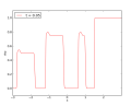
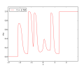
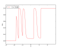
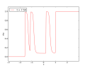
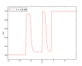
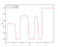
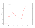
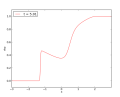
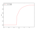
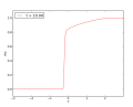
Figure 1: Integration of (1.1)–(3.1)–(3.3) in the two cases (3.2) at times $t=0.05$, $2.50$, $5.01$, $7.50$, $10.00$. Above, drivers look backward while below they look forward. Note, already on the first column, the difference in the two evolutions, clearly due to the position of the support of $\eta$.

However, the qualitative behaviors of the solutions are rather different in the two situations in (3.2), see Figure 1. Clearly, the evolution in the case of drivers looking forward (second line in Figure 1) is far more reasonable, while the backward looking case leads to big oscillations in the vehicular density.

3.2 Increase of the Total Variation and of the ${\mathbf{L}^{\infty}}$ Norm

This paragraph is devoted to show that Lemma 2.2 and the total variation bound (2.12) are, at least qualitatively, optimal. Moreover, the example below shows that the nonlocal equation (1.1) does not enjoy two standard properties typical of 1D scalar conservation laws, namely the maximum principle [1, (iv) in Theorem 6.3], see also [12, Theorem 3], and the diminishing of the total variation [1, Theorem 6.1].

In Remark 2.3 the assumption that $f(\bar{\rho})=0$ can not be replaced by $v(\bar{\rho})=0$ to ensure that the solution remains bounded between $0$ and $\bar{\rho}$. Let $\bar{\rho}=1$ and consider (1.1) in the case

$$f(\rho)=\rho\,,\qquad v(r)=1-r\quad\mbox{ and }\quad\eta(x)=\alpha\left((x-a)(b-x)\right)^{5/2}\,\chi_{[a,b]}(x)$$ (3.4)

with $\alpha$ chosen so that $\int_{{\mathbb{R}}}\eta=1$. Then, clearly, the initial data $\bar{\rho}(x)\equiv 1$ and $\bar{\rho}(x)\equiv 0$ are stationary solutions to (1.1)–(3.4). However, as the numerical integration below shows, the initial datum

$$\rho^{o}(x)=0.25\,\chi_{[-1.35,\,-0,95]}(x)+\chi_{[-0.85,\,-0.25]}(x)+0.75\,\chi_{[-0.15,\,.25]}(x)$$ (3.5)

which satisfies $\rho^{o}(x)\in[0,1]$ for all $x\in{\mathbb{R}}$, yields a solution $\rho=\rho(t,x)$ that exceeds $\bar{\rho}=1$, showing that (1.1)–(3.4) does not satisfy the Maximum Principle, see Figure 2.

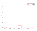
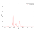
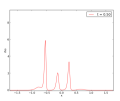
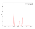
Figure 2: Numerical integration of (1.1)–(3.4) with $a=0$, $b=0.2$ and with the initial datum (3.5) at times $t=0.00,\,0.25,\,0.50,\,0.75,\,1.00$. Note the sharp increase in both the ${\mathbf{L}^{\infty}}$–norm and in the total variation.

Remark that the choice (3.4) leads to a flow in (1.1) which is independent both from $t$ and $x$. In the standard case of local scalar conservation laws, [1, Theorem 6.1] ensures that the total variation of the solution may not increase in time. The numerical integration below shows that the total variation of the solution to (1.1)–(3.4) may well sharply increase in a very short time, coherently with (2.12).

It is of interest to note that this behavior depends from the geometry of the support of $\eta$. Indeed, a translation of the convolution kernel leads to very different solutions, see Figure 3.

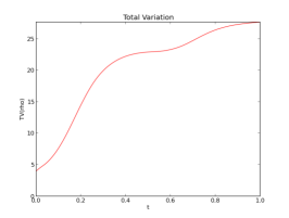
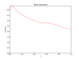
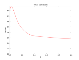
Figure 3: Total variation of the solution to (1.1)–(3.4)–(3.5) versus time, in the three cases $a=0,\,b=0.2$; $a=-0.1,\,b=0.1$ and $a=-0.2,\,b=0$. Remark that the vertical scales in the leftmost diagram differs from that used in the middle and on the right. Indeed, the initial total variation is the same, $4$, in all cases.

When the support is contained in ${\mathbb{R}}^{+}$, there is a sharp increase in the total variation. In the other two cases, when $\mathop{\rm spt}\eta$ is centered about the origin or contained in ${\mathbb{R}}^{-}$, there is a small increase in $\mathinner{\rm TV}(\rho)$ for a small time interval, with a subsequent decrease.

3.3 The Nonlocal to Local Limit

In this section we use the algorithm (2.9) to investigate the limit in which $\eta$ tends to a Dirac $\delta$, so that the nonlocal equation (1.1) tends, at least formally, to the local conservation law (1.2). To our knowledge, no analytical result is at present available on this limit.

Consider (1.1) with the initial datum and the parameters below, see also Figure 4, left:

$$\begin{array}[]{@{}r@{\;}c@{\;}l@{}@{\qquad}@{}r@{\;}c@{\;}l@{}}f(t,x,\rho)&=&\rho&v(r)&=&(1-r)^{3}\,\chi_{]-\infty,1[}(r)\\[10.0pt] \eta_{a}(x)&=&\alpha_{a}\,(a^{2}-x^{2})^{5/2}\,\chi_{[-a,a]}(x)&\rho_{o}(x)&=&\frac{3}{4}\,\chi_{[-1.8,-1.3[}(x)+\chi_{[-1.3,\,-0.8]}(x)\,,\end{array}$$ (3.6)

and with the following choices for $a$:

$$a=0.25,\quad 0.1,\quad 0.05,$$

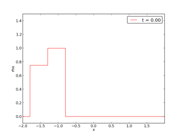
Figure 4: Left, the initial datum in (3.6) and, right, the flow (3.6) used in (1.2). Note its change of convexity.

with $\alpha_{a}$ computed so that $\int_{{\mathbb{R}}}\eta_{a}(x)\mathinner{\mathrm{d}{x}}=1$. As limit case, we consider the standard conservation law (1.2) with $f$ and $v$ as in (3.6), see also Figure 4, right.

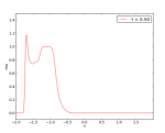
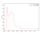
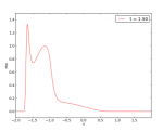
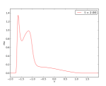
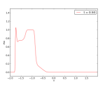
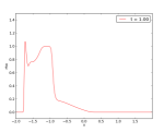
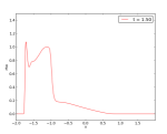
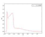
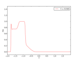
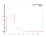
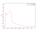
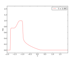
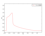
Figure 5: Integration of (1.1)–(3.6), first row with $a=0.25$, second with $a=0.1$, third with $a=0.05$. On the last row, integration of (1.2)–(3.6). The four columns display the times $t=0.5,\,1.0,\,1.5$ and $2.0$. The mixed waves are due to the non-convex flow (3.6), see Figure 4.

In the integration below, the solution $\rho$ attains positive values, so that after an easy modification of $v$ on ${\mathbb{R}}^{-}$ we can assume that (2.6) holds.

The resulting numerical integrations, carried out satisfying the CFL condition (2.8), give the diagrams in Figure 5. In the limit case of (1.2), the chosen initial datum leads to the formation of a rarefaction wave, a shock and a mixed wave, due to the change of convexity of the flow, see the lowest line in Figure 5. The numerical integrations shown in Figure 5 qualitatively suggest that in the limit $a\to 0$ the solution to (1.1)–(3.6) converges to that of (1.2)–(3.6).

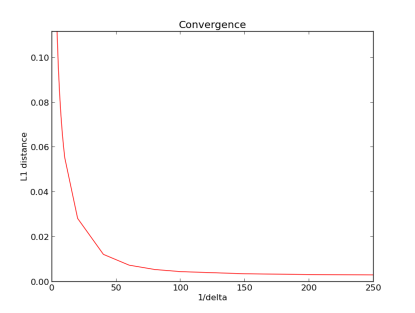
Figure 6: ${\mathbf{L}^{1}}$-distance between the solution $\rho_{a}$ to (1.1)–(3.6) for the values of $a$ in (3.7) and the solution $\rho$ to (1.2)–(3.6) at time $t=0.500$.

A more quantitative hint in this direction is in Figure 6. Using the algorithm above, we computed the solution $\rho_{a}$ to (1.1)–(3.6) for different values of $a$ and the solution $\rho$ to (1.2)–(3.6), all at time $t=0.500$. Figure 6 presents the plot of the ${\mathbf{L}^{1}}$–distance ${\left\|\rho_{a}-\rho\right\|}_{{\mathbf{L}^{1}}}$ versus $1/a$, see also table (3.7).

$$\begin{array}[]{@{}clllll@{}}1/a&4&5&6&7&8\\ {\left\|\rho_{a}-\rho\right\|}_{{\mathbf{L}^{1}}}&0.11166027&0.09569174&0.08373053&0.0743367&0.06674645\\[5.0pt] 1/a&9&10&20&40&60\\ {\left\|\rho_{a}-\rho\right\|}_{{\mathbf{L}^{1}}}&0.06049835&0.05526474&0.0282456&0.0122137&0.0073903\\[5.0pt] 1/a&80&100&150&200&250\\ {\left\|\rho_{a}-\rho\right\|}_{{\mathbf{L}^{1}}}&0.0054428&0.00449935&0.00354348&0.00319927&0.0030382\end{array}$$ (3.7)

4 Technical Details

For any $a,b\in{\mathbb{R}}$, we denote $I(a,b)=\left]a,b\right[\cup\left]b,a\right[$. We use below the following classical notations:

$$D^{+}a_{j}=a_{j+1}-a_{j},\qquad D^{-}a_{j}=a_{j}-a_{j-1},\qquad D^{2}a_{j}=a_{j+1}-2a_{j}+a_{j-1}=(D^{+}-D^{-})a_{j}$$

and recall the trivial identities

$$\begin{array}[]{c}D^{+}(a_{j}b_{j})=(D^{+}a_{j})b_{j+1}+(D^{+}b_{j})a_{j},\qquad\qquad D^{-}(a_{j}b_{j})=(D^{-}a_{j})b_{j}+(D^{-}b_{j})a_{j-1},\\[6.0pt] D^{2}(a_{j}b_{j})=(D^{2}a_{j})b_{j}+(D^{2}b_{j})a_{j}+D^{+}a_{j}D^{+}b_{j}+D^{-}a_{j}D^{-}b_{j}.\end{array}$$

For later use, we note that the algorithm (2.9) can then be rewritten as

$$\rho^{n+1}_{j}=\rho^{n}_{j}-\lambda\,\frac{D^{+}\!\left(f(t^{n},x_{j-1/2},\rho^{n}_{j})\,v(c_{j-1/2})\right)+D^{-}\!\left(f(t^{n},x_{j+1/2},\rho^{n}_{j})\,v(c_{j+1/2})\right)}{2}+\frac{1}{6}\,D^{2}\rho^{n}_{j}\,.$$

Proof of Lemma 2.2.  Note that, by (2.9), standard computations lead to

$$\rho^{n+1}_{j}=(1-\alpha^{n}_{j}-\beta^{n}_{j})\rho^{n}_{j}+\alpha^{n}_{j}\rho^{n}_{j-1}+\beta^{n}_{j}\rho^{n}_{j+1}-\lambda\left(\mathbf{f}^{n}_{j+1/2}(\rho^{n}_{j},\rho^{n}_{j})-\mathbf{f}^{n}_{j-1/2}(\rho^{n}_{j},\rho^{n}_{j})\right).$$ (4.1)

where

$$\alpha^{n}_{j}=\lambda\,\frac{\mathbf{f}^{n}_{j+1/2}(\rho^{n}_{j},\rho^{n}_{j+1})-\mathbf{f}^{n}_{j+1/2}(\rho^{n}_{j},\rho^{n}_{j})}{\rho^{n}_{j+1}-\rho^{n}_{j}}\quad\mbox{ and }\quad\beta^{n}_{j}=\lambda\,\frac{\mathbf{f}^{n}_{j-1/2}(\rho^{n}_{j-1},\rho^{n}_{j})-\mathbf{f}^{n}_{j-1/2}(\rho^{n}_{j},\rho^{n}_{j})}{\rho^{n}_{j-1}-\rho^{n}_{j}}\,.$$ (4.2)

We now show that under condition (2.8), the following inequalities hold:

$$\begin{array}[]{rcl}\alpha^{n}_{j}&\in&[0,1/3]\\ \beta^{n}_{j}&\in&[0,1/3]\\ 1-\alpha^{n}_{j}-\beta^{n}_{j}&\in&[1/3,1]\end{array}\qquad\mbox{ and }\qquad\lambda\,\left(\mathbf{f}^{n}_{j+1/2}(\rho^{n}_{j},\rho^{n}_{j})-\mathbf{f}^{n}_{j-1/2}(\rho^{n}_{j},\rho^{n}_{j})\right)\leq\frac{1}{3}\,\rho^{n}_{j}\,.$$ (4.3)

Indeed,

$$\alpha^{n}_{j} = -\lambda\frac{\mathbf{f}^{n}_{j+1/2}(\rho^{n}_{j},\rho^{n}_{j+1})-\mathbf{f}^{n}_{j+1/2}(\rho^{n}_{j},\rho^{n}_{j})}{\rho^{n}_{j+1}-\rho^{n}_{j}}$$

$$= -\frac{\lambda}{2}\left(\frac{f(t^{n},x_{j+1/2},\rho^{n}_{j+1})-f(t^{n},x_{j+1/2},\rho^{n}_{j})}{\rho^{n}_{j+1}-\rho^{n}_{j}}\,v(c^{n}_{j+1/2})-\frac{1}{3\,\lambda}\right)$$

$$= -\frac{\lambda}{2}\;\partial_{\rho}f(t^{n},x_{j+1/2},\zeta_{j+1/2})\;v(c^{n}_{j+1/2})+\frac{1}{6},$$

So that

$$\alpha^{n}_{j} \geq \displaystyle\frac{1}{2}\left(\frac{1}{3}-\lambda\,{\left\|\partial_{\rho}f\right\|}_{{\mathbf{L}^{\infty}}}\,{\left\|v\right\|}_{{\mathbf{L}^{\infty}}}\right)\;\geq\;0$$

$$\alpha^{n}_{j} \leq \displaystyle\frac{1}{2}\left(\frac{1}{3}+\lambda\,{\left\|\partial_{\rho}f\right\|}_{{\mathbf{L}^{\infty}}}\,{\left\|v\right\|}_{{\mathbf{L}^{\infty}}}\right)\;\leq\;\displaystyle\frac{1}{6}\,.$$ (4.4)

Entirely similar computations lead to analogous estimates for $\beta^{n}_{j}$. The bounds on $1-\alpha^{n}_{j}-\beta^{n}_{j}$ follow. The last term in (4.3), using (2.10) and (2.7), is estimated as follows

$$\mathbf{f}^{n}_{j+1/2}(\rho^{n}_{j},\rho^{n}_{j})-\mathbf{f}^{n}_{j-1/2}(\rho^{n}_{j},\rho^{n}_{j})$$

$$\leq {\left|f(t^{n},x_{j+1/2},\rho^{n}_{j})\,v(c^{n}_{j+1/2})-f(t^{n},x_{j-1/2},\rho^{n}_{j})\,v(c^{n}_{j-1/2})\right|}$$

$$\leq {\left|f(t^{n},x_{j+1/2},\rho^{n}_{j})-f(t^{n},x_{j-1/2},\rho^{n}_{j})\right|}v(c^{n}_{j-1/2})+{\left|f(t^{n},x_{j-1/2},\rho^{n}_{j})\right|}{\left|v(c^{n}_{j+1/2})-v(c^{n}_{j-1/2})\right|}$$

$$\leq h\,{\left|\partial_{x}f(t^{n},\zeta_{j},\rho^{n}_{j})\right|}\,{\left\|v\right\|}_{{\mathbf{L}^{\infty}}}+2\,{\left\|\partial_{\rho}f\right\|}_{{\mathbf{L}^{\infty}}}\,{\left\|v\right\|}_{{\mathbf{L}^{\infty}}}\,{\left|\rho^{n}_{j}\right|}$$

$$\leq \left(C\,{\left\|v\right\|}_{{\mathbf{L}^{\infty}}}\,h+2\,{\left\|\partial_{\rho}f\right\|}_{{\mathbf{L}^{\infty}}}\,{\left\|v\right\|}_{{\mathbf{L}^{\infty}}}\right){\left|\rho^{n}_{j}\right|}$$

$$\leq \left(1+2\,{\left\|\partial_{\rho}f\right\|}_{{\mathbf{L}^{\infty}}}\right){\left\|v\right\|}_{{\mathbf{L}^{\infty}}}\,{\left|\rho^{n}_{j}\right|}$$

$$\leq \frac{1}{3\,\lambda}\,\rho^{n}_{j}\,.$$

Using the bounds (4.3) in (4.1), we obtain

$$\rho^{n+1}_{j}\geq(1-\alpha^{n}_{j}-\beta^{n}_{j})\,\rho^{n}_{j}+\alpha^{n}_{j}\,\rho^{n}_{j-1}+\beta^{n}_{j}\,\rho^{n}_{j+1}-\frac{1}{3}\,\rho^{n}_{j}\geq 0\,,$$

proving the positivity of the discrete solution.   $\square$

Proof of Lemma 2.4.  Thanks to the positivity of the discrete solution, it is sufficient to compute

$${\left\|\rho^{n+1}\right\|}_{{\mathbf{L}^{1}}} = \sum_{j}h\,\rho^{n+1}_{j}$$

$$= \sum_{j}h\left(\rho^{n}_{j}-\lambda\left(\mathbf{f}^{n}_{j+1/2}(\rho^{n}_{j},\rho^{n}_{j+1})-\mathbf{f}^{n}_{j-1/2}(\rho^{n}_{j-1},\rho^{n}_{j})\right)\right)$$

$$= \sum_{j}h\,\rho^{n}_{j}-h\,\lambda\,\left(\lim_{i\to-\infty}\mathbf{f}^{n}_{i+1/2}(\rho^{n}_{i},\rho^{n}_{i+1})-\lim_{i\to+\infty}\mathbf{f}^{n}_{i-1/2}(\rho^{n}_{i-1},\rho^{n}_{i})\right)$$

$$= {\left\|\rho^{n}\right\|}_{{\mathbf{L}^{1}}}$$

completing the proof.   $\square$

Proof of Lemma 2.5.  For later use, estimate the quantity

$${\left|c^{n}_{j+1/2}-c^{n}_{j-1/2}\right|} \leq \sum_{k\in{\mathbb{Z}}}h\,{\left|\rho^{n}_{k+1/2}(\eta_{k-(j+1/2)}-\eta_{k-(j-1/2)})\right|}$$

$$\leq \sum_{k\in{\mathbb{Z}}}h\,\rho^{n}_{k+1/2}\int_{x_{k-j-1/2}}^{x_{k-j+1/2}}{\left|\eta^{\prime}(s)\right|}\,ds$$

$$\leq h\,{\left\|\rho^{n}\right\|}_{{\mathbf{L}^{1}}}\,{\left\|\eta^{\prime}\right\|}_{{\mathbf{L}^{\infty}}}$$

$$= h\,{\left\|\rho^{o}\right\|}_{{\mathbf{L}^{1}}}\,{\left\|\eta^{\prime}\right\|}_{{\mathbf{L}^{\infty}}}\,,$$

where Lemma 2.4 was used. Using the same estimates as in the proof of Lemma 2.2, equality (4.1) yields

$$\rho^{n+1}_{j} \leq (1-\alpha^{n}_{j}-\beta^{n}_{j})\,\rho^{n}_{j}+\alpha^{n}_{j}\,\rho^{n}_{j-1}+\beta^{n}_{j}\,\rho^{n}_{j+1}$$

$$+\lambda{\left|f(t^{n},x_{j+1/2},\rho^{n}_{j})-f(t^{n},x_{j-1/2},\rho^{n}_{j})\right|}\,v(c^{n}_{j-1/2})$$

$$+\lambda{\left|f(t^{n},x_{j-1/2},\rho^{n}_{j})\right|}\,{\left|D^{-}v(c^{n}_{j+1/2})\right|}$$

$$\leq (1-\alpha^{n}_{j}-\beta^{n}_{j})\,{\left\|\rho^{n}\right\|}_{{\mathbf{L}^{\infty}}}+\alpha^{n}_{j}\,{\left\|\rho^{n}\right\|}_{{\mathbf{L}^{\infty}}}+\beta^{n}_{j}\,{\left\|\rho^{n}\right\|}_{{\mathbf{L}^{\infty}}}$$

$$+\lambda\left(h\,{\left|\partial_{x}f(t^{n},\zeta_{j},\rho^{n}_{j})\right|}\,{\left\|v\right\|}_{{\mathbf{L}^{\infty}}}+\rho^{n}_{j}\,{\left\|\partial_{\rho}f\right\|}_{{\mathbf{L}^{\infty}}}\,{\left\|v^{\prime}\right\|}_{{\mathbf{L}^{\infty}}}\,{\left|c^{n}_{j+1/2}-c^{n}_{j-1/2}\right|}\right)$$

$$\leq {\left\|\rho^{n}\right\|}_{{\mathbf{L}^{\infty}}}+\tau\left(C\,{\left\|v\right\|}_{{\mathbf{L}^{\infty}}}+{\left\|\partial_{\rho}f\right\|}_{{\mathbf{L}^{\infty}}}\,{\left\|v^{\prime}\right\|}_{{\mathbf{L}^{\infty}}}\,{\left\|\rho^{o}\right\|}_{{\mathbf{L}^{1}}}\,{\left\|\eta^{\prime}\right\|}_{{\mathbf{L}^{\infty}}}\right){\left\|\rho^{n}\right\|}_{{\mathbf{L}^{\infty}}}$$

$$\leq e^{\mathcal{L}\tau}\,{\left\|\rho^{n}\right\|}_{{\mathbf{L}^{\infty}}}$$

provided

$$\mathcal{L}=C\,{\left\|v\right\|}_{{\mathbf{L}^{\infty}}}+{\left\|\partial_{\rho}f\right\|}_{{\mathbf{L}^{\infty}}}\,{\left\|v^{\prime}\right\|}_{{\mathbf{L}^{\infty}}}\,{\left\|\rho^{o}\right\|}_{{\mathbf{L}^{1}}}\,{\left\|\eta^{\prime}\right\|}_{{\mathbf{L}^{\infty}}}\,.$$ (4.5)

A standard iterative argument completes the proof.   $\square$

Proof of Proposition 2.6.  First, we write (2.9) for $j$ and for $j+1$, subtract and get

$$\rho^{n+1}_{j+1}-\rho^{n+1}_{j}=\rho^{n}_{j+1}-\rho^{n}_{j}$$

$$-\lambda\left(\mathbf{f}^{n}_{j+3/2}(\rho^{n}_{j+1},\rho^{n}_{j+2})-\mathbf{f}^{n}_{j+1/2}(\rho^{n}_{j},\rho^{n}_{j+1})+\mathbf{f}^{n}_{j+1/2}(\rho^{n}_{j},\rho^{n}_{j+1})-\mathbf{f}^{n}_{j-1/2}(\rho^{n}_{j-1},\rho^{n}_{j})\right).$$

Now add and subtract $\mathbf{f}^{n}_{j+3/2}(\rho^{n}_{j},\rho^{n}_{j+1})+\mathbf{f}^{n}_{j+1/2}(\rho^{n}_{j-1},\rho^{n}_{j})$, then rearrange to obtain

$$\rho^{n+1}_{j+1}-\rho^{n+1}_{j}=\mathcal{A}^{n}_{j}-\lambda\,\mathcal{B}^{n}_{j}$$ (4.6)

where

$$\mathcal{A}^{n}_{j} = \rho^{n}_{j+1}-\rho^{n}_{j}$$

$$-\lambda\left(\mathbf{f}^{n}_{j+3/2}(\rho^{n}_{j+1},\rho^{n}_{j+2})-\mathbf{f}^{n}_{j+1/2}(\rho^{n}_{j},\rho^{n}_{j+1})-\mathbf{f}^{n}_{j+3/2}(\rho^{n}_{j},\rho^{n}_{j+1})+\mathbf{f}^{n}_{j+1/2}(\rho^{n}_{j-1},\rho^{n}_{j})\right)$$

$$\mathcal{B}^{n}_{j} = \mathbf{f}^{n}_{j+3/2}(\rho^{n}_{j},\rho^{n}_{j+1})-\mathbf{f}^{n}_{j+1/2}(\rho^{n}_{j},\rho^{n}_{j+1})+\mathbf{f}^{n}_{j-1/2}(\rho^{n}_{j-1},\rho^{n}_{j})-\mathbf{f}^{n}_{j+1/2}(\rho^{n}_{j-1},\rho^{n}_{j})\,.$$ (4.7)

Consider first the term $\mathcal{A}^{n}_{j}$. Recall (4.2) and observe that, after suitable rearrangements,

$$\mathcal{A}^{n}_{j}$$ (4.8)

$$= \frac{2}{3}\,(\rho^{n}_{j+1}-\rho^{n}_{j})$$

$$+ (\rho^{n}_{j+2}-\rho^{n}_{j+1})\left(\frac{1}{6}-\frac{\lambda}{2}\,\frac{f(t^{n},x_{j+3/2},\rho^{n}_{j+2})\,v(c^{n}_{j+3/2})-f(t^{n},x_{j+1/2},\rho^{n}_{j+1})\,v(c^{n}_{j+1/2})}{\rho^{n}_{j+2}-\rho^{n}_{j+1}}\right)$$

$$+ (\rho^{n}_{j}-\rho^{n}_{j-1})\left(\frac{1}{6}+\frac{\lambda}{2}\,\frac{f(t^{n},x_{j+3/2},\rho^{n}_{j})\,v(c^{n}_{j+3/2})-f(t^{n},x_{j+1/2},\rho^{n}_{j-1})\,v(c^{n}_{j+1/2})}{\rho^{n}_{j}-\rho^{n}_{j-1}}\right)$$

$$= \frac{2}{3}\,(\rho^{n}_{j+1}-\rho^{n}_{j})$$

$$+ \!\!(\rho^{n}_{j+2}-\rho^{n}_{j+1})\left[\frac{1}{6}-\frac{\lambda}{2}\frac{f(t^{n},x_{j+3/2},\rho^{n}_{j+2})v(c^{n}_{j+3/2})-f(t^{n},x_{j+3/2},\rho^{n}_{j+1})v(c^{n}_{j+3/2})}{\rho^{n}_{j+2}-\rho^{n}_{j+1}}\right]$$

$$+ (\rho^{n}_{j}-\rho^{n}_{j-1})\left[\frac{1}{6}+\frac{\lambda}{2}\,\frac{f(t^{n},x_{j+3/2},\rho^{n}_{j})\,v(c^{n}_{j+3/2})-f(t^{n},x_{j+3/2},\rho^{n}_{j-1})\,v(c^{n}_{j+3/2})}{\rho^{n}_{j}-\rho^{n}_{j-1}}\right]$$ (4.9)

$$+ -\frac{\lambda}{2}\left(f(t^{n},x_{j+3/2},\rho^{n}_{j+1})-f(t^{n},x_{j+3/2},\rho^{n}_{j-1})\right)v(c^{n}_{j+3/2})$$ (4.10)

$$+ \frac{\lambda}{2}\left(f(t^{n},x_{j+1/2},\rho^{n}_{j+1})-f(t^{n},x_{j+1/2},\rho^{n}_{j-1})\right)v(c^{n}_{j+1/2}).$$ (4.11)

Remark that the term (4.8) equals $\alpha^{n}_{j+1}$, as defined in (4.2). Hence, it can be bounded using (4.3) as follows:

$${\left|\eqref{eq:u1}\right|}\leq\frac{1}{6}\,{\left|\rho^{n}_{j+2}-\rho^{n}_{j+1}\right|}.$$

The estimate for the term (4.9) is exactly as that of $\alpha^{n}_{j}$ in Lemma 2.2, so that

$${\left|\eqref{eq:u2}\right|}\leq\frac{1}{6}\,{\left|\rho^{n}_{j}-\rho^{n}_{j-1}\right|}.$$

Consider now the terms (4.10) and (4.11):

$$\eqref{eq:u3}+\eqref{eq:u4} = \frac{\lambda}{2}\int_{\rho^{n}_{j-1}}^{\rho^{n}_{j+1}}\left(-\partial_{\rho}f(t^{n},x_{j+3/2},r)\,v(c^{n}_{j+3/2})+\partial_{\rho}f(t^{n},x_{j+1/2},r)\,v(c^{n}_{j+1/2})\right)\mathinner{\mathrm{d}{r}}$$

$$= -\frac{\lambda}{2}\int_{\rho^{n}_{j-1}}^{\rho^{n}_{j+1}}\left(\partial_{\rho}f(t^{n},x_{j+3/2},r)-\partial_{\rho}f(t^{n},x_{j+1/2},r)\right)\mathinner{\mathrm{d}{r}}\;v(c^{n}_{j+3/2})$$

$$\qquad-\frac{\lambda}{2}\int_{\rho^{n}_{j-1}}^{\rho^{n}_{j+1}}\partial_{\rho}f(t^{n},x_{j+1/2},r)\mathinner{\mathrm{d}{r}}\;\left(v(c^{n}_{j+3/2})-v(c^{n}_{j+1/2})\right)$$

$$= -\frac{\lambda}{2}\int_{\rho^{n}_{j-1}}^{\rho^{n}_{j+1}}\int_{x_{j+1/2}}^{x_{j+3/2}}\partial^{2}_{x,\rho}f(t^{n},\xi,r)\,\mathinner{\mathrm{d}{\xi}}\,\mathinner{\mathrm{d}{r}}\;v(c^{n}_{j+3/2})$$

$$-\frac{\lambda}{2}\int_{\rho^{n}_{j-1}}^{\rho^{n}_{j+1}}\partial_{\rho}f(t^{n},x_{j+1/2},r)\mathinner{\mathrm{d}{r}}\;\left(v(c^{n}_{j+3/2})-v(c^{n}_{j+1/2})\right)$$

So that, passing to the absolute value

$${\left|\eqref{eq:u3}+\eqref{eq:u4}\right|}\leq\frac{1}{2}\left[{\left\|\partial^{2}_{x,\rho}f\right\|}_{{\mathbf{L}^{\infty}}}\,{\left\|v\right\|}_{{\mathbf{L}^{\infty}}}+{\left\|\partial_{\rho}f\right\|}_{{\mathbf{L}^{\infty}}}\,{\left\|v^{\prime}\right\|}_{{\mathbf{L}^{\infty}}}\,{\left\|\rho^{o}\right\|}_{{\mathbf{L}^{1}}}\,{\left\|\eta^{\prime}\right\|}_{{\mathbf{L}^{\infty}}}\right]\tau\,{\left|\rho^{n}_{j+1}-\rho^{n}_{j-1}\right|}$$

Grouping the estimates obtained we get

$$\begin{array}[]{@{}rcl@{}}\sum_{j\in{\mathbb{Z}}}{\left|\mathcal{A}^{n}_{j}\right|}&\leq&\left[1+\frac{1}{2}\left({\left\|\partial^{2}_{x,\rho}f\right\|}_{{\mathbf{L}^{\infty}}}\,{\left\|v\right\|}_{{\mathbf{L}^{\infty}}}+{\left\|\partial_{\rho}f\right\|}_{{\mathbf{L}^{\infty}}}\,{\left\|v^{\prime}\right\|}_{{\mathbf{L}^{\infty}}}\,{\left\|\rho^{o}\right\|}_{{\mathbf{L}^{1}}}\,{\left\|\eta^{\prime}\right\|}_{{\mathbf{L}^{\infty}}}\right)\,\tau\right]\\ &&\qquad\qquad\times\sum_{j\in{\mathbb{Z}}}{\left|\rho^{n}_{j+1}-\rho^{n}_{j}\right|}\,.\end{array}$$ (4.12)

We now turn to the term $\mathcal{B}^{n}_{j}$ in (4.7). Since

$$\!\!\!\!\!\!\!\!\!\mathcal{B}^{n}_{j} = \frac{f(t^{n},x_{j+3/2},\rho^{n}_{j})v(c_{j+3/2})-2f(t^{n},x_{j+1/2},\rho^{n}_{j})v(c_{j+1/2})+f(t^{n},x_{j-1/2},\rho^{n}_{j})v(c_{j-1/2})}{2}$$ (4.15)

$$+\frac{f(t^{n},x_{j+3/2},\rho^{n}_{j+1})\,v(c_{j+3/2})-f(t^{n},x_{j+1/2},\rho^{n}_{j+1})\,v(c_{j+1/2})}{2}$$

$$-\frac{f(t^{n},x_{j+1/2},\rho^{n}_{j-1})\,v(c_{j+1/2})-f(t^{n},x_{j-1/2},\rho^{n}_{j-1})\,v(c_{j-1/2})}{2}\,,$$

we consider the various terms separately.

$$\eqref{eq:uu1} = v(c_{j+1/2})\;\frac{f(t^{n},x_{j+3/2},\rho^{n}_{j})-2f(t^{n},x_{j+1/2},\rho^{n}_{j})+f(t^{n},x_{j-1/2},\rho^{n}_{j})}{2}$$

$$+f(t^{n},x_{j+1/2},\rho^{n}_{j})\;\frac{v(c_{j+3/2})-2v(c_{j+1/2})+v(c_{j-1/2})}{2}$$

$$+\frac{f(t^{n},x_{j+3/2},\rho^{n}_{j})-f(t^{n},x_{j+1/2},\rho^{n}_{j})}{2}\;\frac{v(c_{j+3/2})-v(c_{j+1/2})}{2}$$

$$+\frac{f(t^{n},x_{j+1/2},\rho^{n}_{j})-f(t^{n},x_{j-1/2},\rho^{n}_{j})}{2}\;\frac{v(c_{j+1/2})-v(c_{j-1/2})}{2}$$

where

$${\left|\frac{f(t^{n},x_{j+3/2},\rho^{n}_{j})-2f(t^{n},x_{j+1/2},\rho^{n}_{j})+f(t^{n},x_{j-1/2},\rho^{n}_{j})}{2}\right|}$$

$$= {\left|\frac{f(t^{n},x_{j+3/2},\rho^{n}_{j})-f(t^{n},x_{j+1/2},\rho^{n}_{j})}{2}-\frac{f(t^{n},x_{j+1/2},\rho^{n}_{j})+f(t^{n},x_{j-1/2},\rho^{n}_{j})}{2}\right|}$$

$$\leq \frac{h}{2}\,{\left|\partial_{x}f(t^{n},\zeta_{j+1},\rho^{n}_{j})-\partial_{x}f(t^{n},\zeta_{j-1},\rho^{n}_{j})\right|}$$

$$\leq \frac{h}{2}\,\int_{\zeta_{j-1}}^{\zeta_{j+1}}{\left|\partial^{2}_{xx}f(t_{x},x,\rho^{n}_{j})\right|}\mathinner{\mathrm{d}{x}}$$

$$\leq C\,h^{2}\,{\left|\rho^{n}_{j}\right|}$$

where (2.5) was used to get to the last line. Moreover,

$$\frac{v(c_{j+3/2})-2v(c_{j+1/2})+v(c_{j-1/2})}{2}$$

$$= \frac{v(c_{j+3/2})-v(c_{j+1/2})}{2}-\frac{v(c_{j+1/2})+v(c_{j-1/2})}{2}$$

$$= \frac{1}{2}\left(v^{\prime}(\zeta_{j})(c^{n}_{j+1/2}-c^{n}_{j-1/2})-v^{\prime}(\zeta_{j+1})(c^{n}_{j+3/2}-c^{n}_{j+1/2})\right)$$

$$= \frac{1}{2}\left(v^{\prime}(\zeta_{j})-v^{\prime}(\zeta_{j+1})\right)(c^{n}_{j+1/2}-c^{n}_{j-1/2})-\frac{1}{2}v^{\prime}(\zeta_{j+1})(c^{n}_{j+3/2}+2c^{n}_{j+1/2}-c^{n}_{j-1/2})$$

$$= \frac{1}{2}\,v^{\prime\prime}(\xi_{j})\,(\zeta_{j}-\zeta_{j+1})\,(c^{n}_{j+1/2}-c^{n}_{j-1/2})-\frac{1}{2}\,v^{\prime}(\zeta_{j+1})\,(c^{n}_{j+3/2}+2c^{n}_{j+1/2}-c^{n}_{j-1/2})\,.$$

Note that we have ${\left|\zeta_{j}-\zeta_{j+1}\right|}\leq{\left|c^{n}_{j+3/2}-c^{n}_{j+1/2}\right|}+{\left|c^{n}_{j+1/2}-c^{n}_{j-1/2}\right|}$, and so using Young’s inequality,

$$\!{\left|\frac{v(c_{j+3/2})-2v(c_{j+1/2})+v(c_{j-1/2})}{2}\right|}\!\!\! \leq \!\!\!\frac{1}{2}{\left\|v^{\prime\prime}\right\|}_{{\mathbf{L}^{\infty}}}\left[\frac{3}{2}{\left|c^{n}_{j+1/2}-c^{n}_{j-1/2}\right|}^{2}+\frac{1}{2}{\left|c^{n}_{j+3/2}-c^{n}_{j+1/2}\right|}^{2}\right]\!$$

$$+\frac{1}{2}{\left\|v^{\prime}\right\|}_{{\mathbf{L}^{\infty}}}\,{\left|c^{n}_{j+3/2}+2c^{n}_{j+1/2}-c^{n}_{j-1/2}\right|}\,.$$

We now estimate the terms involving the discrete derivatives of $c^{n}_{j}$ in the expression above, exploiting the regularity (2.6) of $\eta$. By (2.11), we have

$${\left|c^{n}_{j+1/2}-c^{n}_{j-1/2}\right|} = {\left|\sum_{k\in{\mathbb{Z}}}h\,\rho^{n}_{k+1/2}\,(\eta_{k-(j+1/2)}-\eta_{k-(j-1/2)})\right|}$$ (4.16)

$$\leq \sum_{k\in{\mathbb{Z}}}h\,{\left|\rho^{n}_{k-j-1/2}\right|}\,{\left|\eta_{k+1/2}-\eta_{k-1/2}\right|}$$

$$\leq \sum_{k\in{\mathbb{Z}}}h\,{\left|\rho^{n}_{k-j-1/2}\right|}\int_{x_{k-1/2}}^{x_{k+1/2}}{\left|\eta^{\prime}(s)\right|}\mathinner{\mathrm{d}{s}}$$

$$\leq h\,{\left\|\rho^{n}\right\|}_{{\mathbf{L}^{1}}}\,{\left\|\eta^{\prime}\right\|}_{{\mathbf{L}^{\infty}}}\,.$$

Similarly,

$${\left|c^{n}_{j+3/2}+2c^{n}_{j+1/2}-c^{n}_{j-1/2}\right|} \leq \sum_{k\in{\mathbb{Z}}}h\,{\left|\rho^{n}_{k-j-1/2}\right|}\,{\left|\eta_{k-1/2}-2\eta_{k+1/2}+\eta_{k+3/2}\right|}$$ (4.17)

$$\leq h\,\sum_{k\in{\mathbb{Z}}}h\,{\left|\rho^{n}_{k-j-1/2}\right|}\,{\left|\eta^{\prime}(\zeta_{k+1})-\eta^{\prime}(\zeta_{k})\right|}$$

$$= h\sum_{k\in{\mathbb{Z}}}h\,{\left|\rho^{n}_{k-j-1/2}\right|}\int_{\zeta_{k}}^{\zeta_{k+1}}{\left|\eta^{\prime\prime}(s)\right|}\mathinner{\mathrm{d}{s}}$$

$$\leq h\sum_{k\in{\mathbb{Z}}}h\,{\left|\rho^{n}_{k-j-1/2}\right|}\int_{x_{k-1/2}}^{x_{k+3/2}}{\left|\eta^{\prime\prime}(s)\right|}\mathinner{\mathrm{d}{s}}$$

$$= 2\,h^{2}\,{\left\|\rho^{n}\right\|}_{{\mathbf{L}^{1}}}\,{\left\|\eta^{\prime\prime}\right\|}_{{\mathbf{L}^{\infty}}}\,,$$

to complete the estimate of (4.15) we use the results above to bound the remaining terms

$${\left|\frac{f(t^{n},x_{j+3/2},\rho^{n}_{j})-f(t^{n},x_{j+1/2},\rho^{n}_{j})}{2}\right|} \leq \frac{1}{2}\,h\,C\,{\left|\rho^{n}_{j}\right|}$$

$${\left|\frac{v(c_{j+3/2})-v(c_{j+1/2})}{2}\right|} \leq \frac{1}{2}\,h\,{\left\|v^{\prime}\right\|}_{{\mathbf{L}^{\infty}}}\,{\left\|\eta^{\prime}\right\|}_{{\mathbf{L}^{\infty}}}\,{\left\|\rho^{o}\right\|}_{{\mathbf{L}^{1}}}$$

$${\left|\frac{f(t^{n},x_{j+1/2},\rho^{n}_{j})-f(t^{n},x_{j-1/2},\rho^{n}_{j})}{2}\right|} \leq \frac{1}{2}\,h\,C\,{\left|\rho^{n}_{j}\right|}$$

$${\left|\frac{v(c_{j+1/2})-v(c_{j-1/2})}{2}\right|} \leq \frac{1}{2}\,h\,{\left\|v^{\prime}\right\|}_{{\mathbf{L}^{\infty}}}\,{\left\|\eta^{\prime}\right\|}_{{\mathbf{L}^{\infty}}}\,{\left\|\rho^{o}\right\|}_{{\mathbf{L}^{1}}}$$

and we are now able to complete the estimate of (4.15):

$$\eqref{eq:uu1} \leq h^{2}\,C\,{\left\|v\right\|}_{\mathbf{L}^{\infty}}\,{\left|\rho^{n}_{j}\right|}$$

$$+{\left\|\partial_{\rho}f\right\|}_{{\mathbf{L}^{\infty}}}\,{\left|\rho^{n}_{j}\right|}\left(h^{2}\,{\left\|v^{\prime\prime}\right\|}_{{\mathbf{L}^{\infty}}}{\left\|\rho^{o}\right\|}_{{\mathbf{L}^{1}}}^{2}\,{\left\|\eta^{\prime}\right\|}_{{\mathbf{L}^{\infty}}}+h^{2}\,{\left\|v^{\prime}\right\|}_{{\mathbf{L}^{\infty}}}\,{\left\|\rho^{o}\right\|}_{{\mathbf{L}^{1}}}^{2}\,{\left\|\eta^{\prime\prime}\right\|}_{{\mathbf{L}^{\infty}}}\right)$$

$$+\frac{1}{2}\,h^{2}\,C\,{\left\|v^{\prime}\right\|}_{{\mathbf{L}^{\infty}}}\,{\left\|\eta^{\prime}\right\|}_{{\mathbf{L}^{\infty}}}\,{\left\|\rho^{o}\right\|}_{{\mathbf{L}^{1}}}\,{\left|\rho^{n}_{j}\right|}$$

$$= h^{2}\Big{[}C{\left\|v\right\|}_{\mathbf{L}^{\infty}}+\Big{(}{\left\|\partial_{\rho}f\right\|}_{{\mathbf{L}^{\infty}}}\left({\left\|v^{\prime\prime}\right\|}_{{\mathbf{L}^{\infty}}}{\left\|\eta^{\prime}\right\|}_{{\mathbf{L}^{\infty}}}+{\left\|v^{\prime}\right\|}_{{\mathbf{L}^{\infty}}}{\left\|\eta^{\prime\prime}\right\|}_{{\mathbf{L}^{\infty}}}\right)$$

$$\qquad\qquad\qquad+\frac{C}{2}{\left\|v^{\prime}\right\|}_{{\mathbf{L}^{\infty}}}{\left\|\eta^{\prime}\right\|}_{{\mathbf{L}^{\infty}}}\Big{)}{\left\|\rho^{o}\right\|}_{{\mathbf{L}^{1}}}\Big{]}{\left|\rho^{n}_{j}\right|}$$

$$\leq h^{2}\,{\left\|v\right\|}_{{\mathbf{W}^{2,\infty}}}\left(C+\left({\left\|\partial_{\rho}f\right\|}_{{\mathbf{L}^{\infty}}}+\frac{C}{2}\right){\left\|\eta^{\prime}\right\|}_{{\mathbf{W}^{1,\infty}}}\,{\left\|\rho^{o}\right\|}_{{\mathbf{L}^{1}}}\right){\left|\rho^{n}_{j}\right|}$$

We now pass to estimate (4.15) and (4.15):

$$\eqref{eq:uu2}+\eqref{eq:uu3} = \frac{1}{2}\,\left(f(t^{n},x_{j+3/2},\rho^{n}_{j+1})-f(t^{n},x_{j+1/2},\rho^{n}_{j+1})\right)v(c_{j+3/2})$$

$$+\frac{1}{2}\,f(t^{n},x_{j+1/2},\rho^{n}_{j+1})\left(v(c_{j+3/2})-v(c_{j+1/2})\right)$$

$$-\frac{1}{2}\,\left(f(t^{n},x_{j+1/2},\rho^{n}_{j-1})-f(t^{n},x_{j-1/2},\rho^{n}_{j-1})\right)v(c_{j+1/2})$$

$$-\frac{1}{2}\,f(t^{n},x_{j-1/2},\rho^{n}_{j-1})\left(v(c_{j+1/2})-v(c_{j-1/2})\right)$$

$$= \frac{1}{2}\,h\,\left(\partial_{x}f(t^{n},\xi_{j+1},\rho^{n}_{j+1})\,v(c_{j+3/2})-\partial_{x}f(t^{n},\xi_{j},\rho^{n}_{j-1})\,v(c_{j+1/2})\right)$$

$$+\frac{1}{2}\Big{(}f(t^{n},x_{j+1/2},\rho^{n}_{j+1})\,v^{\prime}(\gamma_{j+1})\,(c_{j+3/2}-c_{j+1/2})$$

$$\qquad\qquad\qquad-f(t^{n},x_{j-1/2},\rho^{n}_{j-1})\,v^{\prime}(\gamma_{j})\,(c_{j+1/2}-c_{j-1/2})\Big{)}$$

for suitable $\xi_{j}\in\left]x_{j-1/2},x_{j+1/2}\right[$ and $\gamma_{j}\in I(c_{j-1/2},c_{j+1/2})$. Introducing $\hat{\xi}_{j}\in\left]\xi_{j},\xi_{j+1}\right[$, $\hat{\zeta}_{j}\in I(\rho^{n}_{j-1},\rho^{n}_{j+1})$, $\hat{\gamma}_{j}\in I(\gamma_{j},\gamma_{j+1})$, $\check{\xi}_{j}\in\left]x_{j-1/2},x_{j+1/2}\right[$, $\check{\zeta}_{j}\in I(\rho^{n}_{j-1},\rho^{n}_{j+1})$, $\check{\gamma}_{j}\in I(\gamma_{j},\gamma_{j+1})$, $\delta_{j}\in I(c_{j+3/2}-c_{j+1/2},c_{j+1/2}-c_{j-1/2})$ and using (2.5), (4.16), (4.17)

$${\left|\eqref{eq:uu2}+\eqref{eq:uu3}\right|}$$

$$\leq \frac{1}{2}\,h\,\Big{(}{\left|\partial^{2}_{xx}f(t^{n},\hat{\xi}_{j},\hat{\zeta}_{j})\right|}\,v(\hat{\gamma}_{j+1})\,h+{\left|\partial^{2}_{\rho x}f(t^{n},\hat{\xi}_{j},\hat{\zeta}_{j})\right|}\,v(\hat{\gamma}_{j+1})\,{\left|\rho^{n}_{j+1}-\rho^{n}_{j-1}\right|}$$

$$\qquad\qquad\qquad+{\left|\partial_{x}f(t^{n},\hat{\xi}_{j},\hat{\zeta}_{j})\right|}\,{\left|v^{\prime}(\hat{\gamma}_{j+1})\right|}\,{\left|c_{j+3/2}-c_{j+1/2}\right|}\Big{)}$$

$$+\frac{1}{2}\,\Big{(}{\left|\partial_{x}f(t^{n},\check{\xi}_{j},\check{\zeta}_{j})\right|}\,{\left|v^{\prime}(\check{\gamma}_{j})\right|}\,{\left|\delta_{j}\right|}\,h+{\left|f(t^{n},\check{\xi}_{j},\check{\zeta}_{j})\right|}\,{\left|v^{\prime\prime}(\check{\gamma}_{j})\right|}\,{\left|\delta_{j}\right|}\,{\left|\gamma_{j+1}-\gamma_{j}\right|}$$

$$\qquad\qquad\qquad+{\left|f(t^{n},\check{\xi}_{j},\check{\zeta}_{j})\right|}\,{\left|v^{\prime}(\check{\gamma}_{j})\right|}\,{\left|c_{j+3/2}-2c_{j+1/2}-c_{j-1/2}\right|}\Big{)}$$

$$\leq \frac{1}{2}\,h\Big{(}C\,{\left\|v\right\|}_{{\mathbf{L}^{\infty}}}\,{\left|\hat{\zeta}_{j}\right|}\,h+{\left\|\partial^{2}_{\rho x}f\right\|}_{{\mathbf{L}^{\infty}}}\,{\left\|v\right\|}_{{\mathbf{L}^{\infty}}}\,{\left|\rho^{n}_{j+1}-\rho^{n}_{j-1}\right|}+C\,{\left\|v^{\prime}\right\|}_{{\mathbf{L}^{\infty}}}\,{\left\|\rho^{o}\right\|}_{{\mathbf{L}^{1}}}\,{\left\|\eta^{\prime}\right\|}_{{\mathbf{L}^{\infty}}}\,{\left|\hat{\zeta}_{j}\right|}\,h\Big{)}$$

$$+\frac{1}{2}\,\Big{(}C\,{\left\|v^{\prime}\right\|}_{{\mathbf{L}^{\infty}}}\,{\left\|\rho^{o}\right\|}_{{\mathbf{L}^{1}}}\,{\left\|\eta^{\prime}\right\|}_{{\mathbf{L}^{\infty}}}\,{\left|\check{\zeta}_{j}\right|}\,h^{2}+{\left\|\partial_{\rho}f\right\|}_{{\mathbf{L}^{\infty}}}\,{\left\|v^{\prime\prime}\right\|}_{{\mathbf{L}^{\infty}}}\,{\left\|\rho^{o}\right\|}_{{\mathbf{L}^{1}}}^{2}\,{\left\|\eta^{\prime}\right\|}_{{\mathbf{L}^{\infty}}}^{2}\,{\left|\check{\zeta}_{j}\right|}\,h^{2}$$

$$\qquad\qquad\qquad+2\,{\left\|\partial_{\rho}f\right\|}_{{\mathbf{L}^{\infty}}}\,{\left\|v^{\prime}\right\|}_{{\mathbf{L}^{\infty}}}\,{\left\|\rho^{o}\right\|}_{{\mathbf{L}^{1}}}\,{\left\|\eta^{\prime\prime}\right\|}_{{\mathbf{L}^{\infty}}}\,{\left|\check{\zeta}_{j}\right|}\,h^{2}\Big{)}$$

$$= \frac{1}{2}\,C\left(1+{\left\|\eta^{\prime}\right\|}_{{\mathbf{L}^{\infty}}}\,{\left\|\rho^{o}\right\|}_{{\mathbf{L}^{1}}}\right){\left\|v\right\|}_{{\mathbf{W}^{1,\infty}}}\,{\left|\hat{\zeta}_{j}\right|}\,h^{2}$$

$$+\frac{1}{2}\left(C\,+{\left\|\partial_{\rho}f\right\|}_{{\mathbf{L}^{\infty}}}\,{\left\|\rho^{o}\right\|}_{{\mathbf{L}^{1}}}\,{\left\|\eta^{\prime}\right\|}_{{\mathbf{L}^{\infty}}}+2\,{\left\|\partial_{\rho}f\right\|}_{{\mathbf{L}^{\infty}}}\right){\left\|v^{\prime}\right\|}_{{\mathbf{W}^{1,\infty}}}\,{\left\|\eta^{\prime}\right\|}_{{\mathbf{W}^{1,\infty}}}\,{\left\|\rho^{o}\right\|}_{{\mathbf{L}^{1}}}\,{\left|\check{\zeta}_{j}\right|}\,h^{2}$$

$$+\frac{1}{2}\,{\left\|\partial^{2}_{\rho x}f\right\|}_{{\mathbf{L}^{\infty}}}\,{\left\|v\right\|}_{{\mathbf{L}^{\infty}}}{\left|\rho^{n}_{j+1}-\rho^{n}_{j-1}\right|}\,h\,.$$

The above bound allows to obtain the estimate for $\mathcal{B}_{j}$:

$$\mathcal{B}_{j} \leq {\left\|v\right\|}_{{\mathbf{W}^{2,\infty}}}\left(C+\left({\left\|\partial_{\rho}f\right\|}_{{\mathbf{L}^{\infty}}}+\frac{C}{2}\right){\left\|\eta^{\prime}\right\|}_{{\mathbf{W}^{1,\infty}}}\,{\left\|\rho^{o}\right\|}_{{\mathbf{L}^{1}}}\right){\left|\rho^{n}_{j}\right|}\,h^{2}$$

$$+\frac{1}{2}\,C\left(1+{\left\|\eta^{\prime}\right\|}_{{\mathbf{L}^{\infty}}}\,{\left\|\rho^{o}\right\|}_{{\mathbf{L}^{1}}}\right){\left\|v\right\|}_{{\mathbf{W}^{1,\infty}}}\,{\left|\hat{\zeta}_{j}\right|}\,h^{2}$$

$$+\frac{1}{2}\left(C\,+{\left\|\partial_{\rho}f\right\|}_{{\mathbf{L}^{\infty}}}\,{\left\|\rho^{o}\right\|}_{{\mathbf{L}^{1}}}\,{\left\|\eta^{\prime}\right\|}_{{\mathbf{L}^{\infty}}}+2\,{\left\|\partial_{\rho}f\right\|}_{{\mathbf{L}^{\infty}}}\right){\left\|v^{\prime}\right\|}_{{\mathbf{W}^{1,\infty}}}\,{\left\|\eta^{\prime}\right\|}_{{\mathbf{W}^{1,\infty}}}\,{\left\|\rho^{o}\right\|}_{{\mathbf{L}^{1}}}\,{\left|\check{\zeta}_{j}\right|}\,h^{2}$$

$$+\frac{1}{2}\,{\left\|\partial^{2}_{\rho x}f\right\|}_{{\mathbf{L}^{\infty}}}\,{\left\|v\right\|}_{{\mathbf{L}^{\infty}}}{\left|\rho^{n}_{j+1}-\rho^{n}_{j-1}\right|}\,h\,.$$

so that

$$\sum_{j\in{\mathbb{Z}}}\mathcal{B}_{j} \leq {\left\|v\right\|}_{{\mathbf{W}^{2,\infty}}}\left(C+\left({\left\|\partial_{\rho}f\right\|}_{{\mathbf{L}^{\infty}}}+\frac{C}{2}\right){\left\|\eta^{\prime}\right\|}_{{\mathbf{W}^{1,\infty}}}\,{\left\|\rho^{o}\right\|}_{{\mathbf{L}^{1}}}\right){\left\|\rho^{o}\right\|}_{{\mathbf{L}^{1}}}\,h$$

$$+\frac{1}{2}\,C\left(1+{\left\|\eta^{\prime}\right\|}_{{\mathbf{L}^{\infty}}}\,{\left\|\rho^{o}\right\|}_{{\mathbf{L}^{1}}}\right){\left\|v\right\|}_{{\mathbf{W}^{1,\infty}}}\,{\left\|\rho^{o}\right\|}_{{\mathbf{L}^{1}}}\,h$$

$$+\frac{1}{2}\left(C\,+{\left\|\partial_{\rho}f\right\|}_{{\mathbf{L}^{\infty}}}\left(2+{\left\|\rho^{o}\right\|}_{{\mathbf{L}^{1}}}\,{\left\|\eta^{\prime}\right\|}_{{\mathbf{L}^{\infty}}}\right)\right){\left\|v^{\prime}\right\|}_{{\mathbf{W}^{1,\infty}}}\,{\left\|\eta^{\prime}\right\|}_{{\mathbf{W}^{1,\infty}}}\,{\left\|\rho^{o}\right\|}_{{\mathbf{L}^{1}}}\,h$$

$$+\frac{1}{2}\,{\left\|\partial^{2}_{\rho x}f\right\|}_{{\mathbf{L}^{\infty}}}\,{\left\|v\right\|}_{{\mathbf{L}^{\infty}}}\left(\sum_{j\in{\mathbb{Z}}}{\left|\rho^{n}_{j+1}-\rho^{n}_{j-1}\right|}\right)h\,.$$

Recall now (4.6) and (4.12) to obtain

$$\sum_{j\in{\mathbb{Z}}}{\left|\rho^{n+1}_{j+1}-\rho^{n+1}_{j}\right|}\leq\sum_{j\in{\mathbb{Z}}}{\left|\mathcal{A}_{j}\right|}+\lambda\sum_{j\in{\mathbb{Z}}}{\left|\mathcal{B}_{j}\right|}\leq(1+\mathcal{K}_{1}\,\tau)\sum_{j\in{\mathbb{Z}}}{\left|\rho^{n}_{j+1}-\rho^{n}_{j}\right|}+\mathcal{K}_{2}\,\tau$$

where

$$\begin{array}[]{rcl}\mathcal{K}_{1}&=&\frac{1}{2}\,{\left\|\partial_{\rho}f\right\|}_{{\mathbf{L}^{\infty}}}\,{\left\|v^{\prime}\right\|}_{{\mathbf{L}^{\infty}}}\,{\left\|\rho^{o}\right\|}_{{\mathbf{L}^{1}}}\,{\left\|\eta^{\prime}\right\|}_{{\mathbf{L}^{\infty}}}+{\left\|\partial^{2}_{\rho x}f\right\|}_{{\mathbf{L}^{\infty}}}\,{\left\|v\right\|}_{{\mathbf{L}^{\infty}}}\\ \mathcal{K}_{2}&=&\Bigg{[}\frac{3}{2}\,C+\left({\left\|\partial_{\rho}f\right\|}_{{\mathbf{L}^{\infty}}}+C\right){\left\|\eta^{\prime}\right\|}_{{\mathbf{W}^{1,\infty}}}\,{\left\|\rho^{o}\right\|}_{{\mathbf{L}^{1}}}\\ &&+\frac{1}{2}\left(C\,+{\left\|\partial_{\rho}f\right\|}_{{\mathbf{L}^{\infty}}}\left(2+{\left\|\rho^{o}\right\|}_{{\mathbf{L}^{1}}}\,{\left\|\eta^{\prime}\right\|}_{{\mathbf{L}^{\infty}}}\right)\right){\left\|\eta^{\prime}\right\|}_{{\mathbf{W}^{1,\infty}}}\Bigg{]}{\left\|v\right\|}_{{\mathbf{W}^{2,\infty}}}\,{\left\|\rho^{o}\right\|}_{{\mathbf{L}^{1}}}\end{array}$$ (4.18)

The estimate (2.12) now follows from standard iterative procedure. The proof of Proposition 2.6 follows immediately.   $\square$

Proof of Lemma 2.7.  We follow the same line as in [11, Section 3]. Using (4.16), Lemma 2.2, Lemma 2.4 and Proposition 2.6 compute preliminarily

$$\sum_{j\in{\mathbb{Z}}}{\left|D^{+}\!\left(f(t^{n},x_{j-1/2},\rho^{n}_{j})\,v(c^{n}_{j-1/2})\right)\right|}$$

$$\leq \sum_{j\in{\mathbb{Z}}}\Big{[}{\left|\partial_{x}f(t^{n},\xi_{j},\zeta_{j})\,v(\gamma_{j})\right|}\,h+{\left|\partial_{\rho}f(t^{n},\xi_{j},\zeta_{j})\,v(\gamma_{j})\right|}\,{\left|\rho^{n}_{j+1}-\rho^{n}_{j}\right|}$$

$$\qquad\qquad+{\left|f(t^{n},\xi_{j},\zeta_{j})\,v^{\prime}(\gamma_{j})\right|}\,{\left|c^{n}_{j+1/2}-c^{n}_{j-1/2}\right|}\Big{]}$$

$$\leq \sum_{j\in{\mathbb{Z}}}\Big{[}C\,{\left\|v\right\|}_{{\mathbf{L}^{\infty}}}\,\rho^{n}_{j}\,h+{\left\|\partial_{\rho}f\right\|}_{{\mathbf{L}^{\infty}}}\,{\left\|v\right\|}_{{\mathbf{L}^{\infty}}}\,{\left|\rho^{n}_{j+1}-\rho^{n}_{j}\right|}$$

$$\qquad\qquad+{\left\|\partial_{\rho}f\right\|}_{{\mathbf{L}^{\infty}}}\,{\left\|v^{\prime}\right\|}_{{\mathbf{L}^{\infty}}}\,{\left\|\eta^{\prime}\right\|}_{{\mathbf{L}^{\infty}}}\,{\left\|\rho^{o}\right\|}_{{\mathbf{L}^{1}}}\,\max\left\{\rho^{n}_{j},\rho^{n}_{j+1}\right\}\,h\Big{]}$$

$$\leq C{\left\|v\right\|}_{{\mathbf{L}^{\infty}}}\,{\left\|\rho^{o}\right\|}_{{\mathbf{L}^{1}}}+2{\left\|\partial_{\rho}f\right\|}_{{\mathbf{L}^{\infty}}}\,{\left\|\rho^{o}\right\|}_{{\mathbf{L}^{1}}}^{2}\,{\left\|\eta^{\prime}\right\|}_{{\mathbf{L}^{\infty}}}{\left\|v^{\prime}\right\|}_{{\mathbf{L}^{\infty}}}\,+{\left\|\partial_{\rho}f\right\|}_{{\mathbf{L}^{\infty}}}{\left\|v\right\|}_{{\mathbf{L}^{\infty}}}\sum_{j\in{\mathbb{Z}}}{\left|\rho^{n}_{j+1}-\rho^{n}_{j}\right|}$$

$$\leq C{\left\|v\right\|}_{{\mathbf{L}^{\infty}}}\,{\left\|\rho^{o}\right\|}_{{\mathbf{L}^{1}}}+2{\left\|\partial_{\rho}f\right\|}_{{\mathbf{L}^{\infty}}}\,{\left\|\rho^{o}\right\|}_{{\mathbf{L}^{1}}}^{2}\,{\left\|\eta^{\prime}\right\|}_{{\mathbf{L}^{\infty}}}{\left\|v^{\prime}\right\|}_{{\mathbf{L}^{\infty}}}$$

$$\qquad\qquad+{\left\|\partial_{\rho}f\right\|}_{{\mathbf{L}^{\infty}}}{\left\|v\right\|}_{{\mathbf{L}^{\infty}}}\left(\mathcal{K}_{2}\,t+\sum_{j\in{\mathbb{Z}}}{\left|\rho^{o}_{j+1}-\rho^{o}_{j}\right|}\right)e^{\mathcal{K}_{1}t}\,.$$

The term $\sum_{j\in{\mathbb{Z}}}{\left|D^{-}\!\left(f(t^{n},x_{j+1/2},\rho^{n}_{j})\,v(c^{n}_{j+1/2})\right)\right|}$ admits an analogous estimate. Moreover,

$$\sum_{j\in{\mathbb{Z}}}{\left|D^{2}\rho^{n}_{j}\right|}\leq 2\sum_{j\in{\mathbb{Z}}}{\left|\rho^{n}_{j+1}-\rho^{n}_{j}\right|}\leq 2\left(\mathcal{K}_{2}\,t+\sum_{j\in{\mathbb{Z}}}{\left|\rho^{o}_{j+1}-\rho^{o}_{j}\right|}\right)e^{\mathcal{K}_{1}t}\,.$$

Using the above estimates and (2.9) we get

$${\left\|\rho^{n+1}-\rho^{n}\right\|}_{{\mathbf{L}^{1}}} = \sum_{j\in{\mathbb{Z}}}h\,{\left|\rho^{n+1}_{j}-\rho^{n}_{j}\right|}$$

$$\leq \frac{\tau}{2}\sum_{j\in{\mathbb{Z}}}{\left|D^{+}\!\left(f(t^{n},x_{j-1/2},\rho^{n}_{j})\,v(c^{n}_{j-1/2})\right)\right|}$$

$$+\frac{\tau}{2}\sum_{j\in{\mathbb{Z}}}{\left|D^{-}\!\left(f(t^{n},x_{j+1/2},\rho^{n}_{j})\,v(c^{n}_{j+1/2})\right)\right|}+\frac{\lambda\,\tau}{6}\sum_{j\in{\mathbb{Z}}}{\left|D^{2}\rho^{n}_{j}\right|}$$

$$\leq {\cal C}(t)\,\tau$$

where

$$\begin{array}[]{rcl}{\cal C}(t)&=&C{\left\|v\right\|}_{{\mathbf{L}^{\infty}}}\,{\left\|\rho^{o}\right\|}_{{\mathbf{L}^{1}}}+2{\left\|\partial_{\rho}f\right\|}_{{\mathbf{L}^{\infty}}}\,{\left\|\rho^{o}\right\|}_{{\mathbf{L}^{1}}}^{2}\,{\left\|\eta^{\prime}\right\|}_{{\mathbf{L}^{\infty}}}{\left\|v^{\prime}\right\|}_{{\mathbf{L}^{\infty}}}\\ &&+\left({\left\|\partial_{\rho}f\right\|}_{{\mathbf{L}^{\infty}}}\,{\left\|v\right\|}_{{\mathbf{L}^{\infty}}}+\frac{\lambda}{3}\right)\left(\mathcal{K}_{2}\,t+\sum_{j\in{\mathbb{Z}}}{\left|\rho^{o}_{j+1}-\rho^{o}_{j}\right|}\right)e^{\mathcal{K}_{1}t}\,,\end{array}$$ (4.19)

completing the proof.   $\square$

Proof of Proposition 2.8.  Fix $n\in{\mathbb{N}}$ and for any sequence $(\rho)_{j\in{\mathbb{Z}}}$ define the transformation $\rho\mapsto H(\rho)$ given by

$$H^{n}_{j}(\rho)=\rho_{j}-\left(\mathbf{f}^{n}_{j+1/2}(\rho_{j},\rho_{j+1})-\mathbf{f}^{n}_{j-1/2}(\rho_{j-1},\rho_{j})\right),$$ (4.20)

where the functions $\mathbf{f}^{n}_{j+1/2}$ are given by (2.10), but where, instead of (2.11), the sequence $(c^{n}_{j+1/2})_{j\in{\mathbb{Z}}}$ is now an arbitrary fixed sequence. Thus, $H^{n}_{j}(\rho)$ depends only on $\rho_{j-1}$, $\rho_{j}$ and $\rho_{j+1}$. Then, $H^{n}$ is monotone, in the sense that

$$\frac{\partial H^{n}_{j}}{\partial\rho_{i}}\geq 0\,,\quad i=j-1,j,j+1.$$ (4.21)

The cases $i=j\pm 1$ are easily verified. If $i=j$, using (2.10) we find

$$\frac{\partial H^{n}_{j}}{\partial\rho_{j}} = \frac{1}{3}-\frac{\lambda}{2}\left(\partial_{\rho}f(t^{n},x_{j+1/2},\rho_{j})\,v(c_{j+1/2})-\partial_{\rho}f(t^{n},x_{j-1/2},\rho_{j})\,v(c_{j-1/2})\right)$$

$$\geq \frac{1}{3}-\lambda\,{\left\|\partial_{\rho}f\right\|}_{{\mathbf{L}^{\infty}}}\,{\left\|v\right\|}_{{\mathbf{L}^{\infty}}}$$

$$\geq 0$$

by the CFL condition (2.8). The definition (4.20) of $H^{n}$ and (2.13) imply that for any $k\in{\mathbb{R}}$

$${\left|\rho_{j}-k\right|}-\lambda\left(F^{k}_{j+1/2}(\rho_{j},\rho_{j+1})-F^{k}_{j-1/2}(\rho_{j-1},\rho_{j})\right)=H^{n}_{j}(\rho\wedge k)-H^{n}_{j}(\rho\vee k)\,,$$ (4.22)

where $k$ in the right-hand side above is understood as the sequence identically equal to $k$. The monotonicity condition (4.21) and the scheme (2.9)–(2.10) ensure that

$$H^{n}_{j}(\rho\wedge k)-H^{n}_{j}(\rho\vee k)$$

$$\geq H^{n}_{j}(\rho)\wedge H^{n}_{j}(k)-H^{n}_{j}(\rho)\vee H^{n}_{j}(k)$$

$$= \mathop{\rm sgn}\left[H^{n}_{j}(\rho)-k+\lambda\left(f(t^{n},x_{j+1/2},k)-f(t^{n},x_{j-1/2},k)\right)\right]\times$$

$$\qquad\times\left[H^{n}_{j}(\rho)-k+\lambda\left(f(t^{n},x_{j+1/2},k)-f(t^{n},x_{j-1/2},k)\right)\right]$$

$$\geq \mathop{\rm sgn}\left(H^{n}_{j}(\rho)-k\right)\left[H^{n}_{j}(\rho)-k+\lambda\left(f(t^{n},x_{j+1/2},k)-f(t^{n},x_{j-1/2},k)\right)\right]$$

$$= {\left|H^{n}_{j}(\rho)-k\right|}+\lambda\,\mathop{\rm sgn}\left(H^{n}_{j}(\rho)-k\right)\left(f(t^{n},x_{j+1/2},k)-f(t^{n},x_{j-1/2},k)\right).$$ (4.23)

In the last inequality we used also the non-negativity of the function $(a,b)\mapsto(\mathop{\rm sgn}(a+b)-\mathop{\rm sgn}(a))(a+b)$. From (4.22) and (4.23) we conclude that

$$\begin{array}[]{rcl}{\left|H^{n}_{j}(\rho)-k\right|}-{\left|\rho_{j}-k\right|}+\lambda\left(F^{k}_{j+1/2}(\rho_{j},\rho_{j+1})-F^{k}_{j-1/2}(\rho_{j-1},\rho_{j})\right)\\ \qquad+\lambda\mathop{\rm sgn}(H^{n}_{j}(\rho)-k)\left(f(t^{n},x_{j+1/2},k)-f(t^{n},x_{j-1/2},k)\right)&\leq&0\,.\end{array}$$ (4.24)

Consider now the numerical approximation $\rho^{n}_{j}$ given by the algorithm (2.9). Then, we apply (4.24) to $\rho^{n}$, with the sequence $c_{j+1/2}$ appearing in (4.20) as given by the convolution (2.11). Observing that $H^{n}_{j}(\rho^{n})=\rho^{n+1}_{j}$, we conclude that (2.14) holds.   $\square$