A Faster Algorithm for Computing Motorcycle Graphs

Abstract

We present a new algorithm for computing motorcycle graphs that runs in $O(n^{4/3+\varepsilon})$ time for any $\varepsilon>0$, improving on all previously known algorithms. The main application of this result is to computing the straight skeleton of a polygon. It allows us to compute the straight skeleton of a non-degenerate polygon with $h$ holes in $O(n\sqrt{h+1}\log^{2}n+n^{4/3+\varepsilon})$ expected time. If all input coordinates are $O(\log n)$-bit rational numbers, we can compute the straight skeleton of a (possibly degenerate) polygon with $h$ holes in $O(n\sqrt{h+1}\log^{3}n)$ expected time.

In particular, it means that we can compute the straight skeleton of a simple polygon in $O(n\log^{3}n)$ expected time if all input coordinates are $O(\log n)$-bit rationals, while all previously known algorithms have worst-case running time $\omega(n^{3/2})$.

1 Introduction

The straight skeleton of a polygon $P$ is a straight line graph embedded in $P$, formed by the traces of the vertices of $P$ when it is shrunk, each edge moving at the same speed and remaining parallel to its original position. (See Figure 1.)

(a) Input polygon

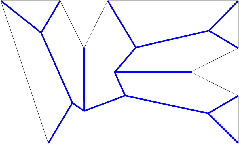
(b) Straight skeleton

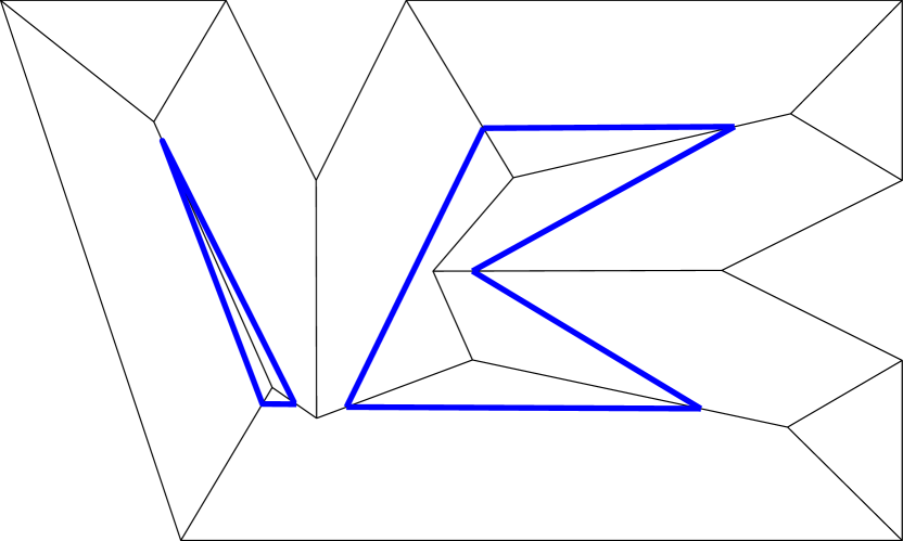
(c) Offset polygon

Figure 1: The straight skeleton of a polygon, and a corresponding offset polygon.

It has been known since at least the 19th century; for instance, figures representing the straight skeleton can be found in the book by von Peschka [32]. Aichholzer et al. [5] gave the first efficient algorithms for computing the straight skeleton, and presented it as an alternative to the medial axis having only straight-line edges. The straight skeleton has found numerous applications in computer science, for instance to city model reconstruction [27], architectural modeling [26], polyhedral surface reconstruction [7, 21, 29], biomedical image processing [16]. It also has a direct application to CAD, as it allows to compute offset polygons [18]. The straight skeleton has become a standard tool in geometric computing, and thus fast and robust software has been developed to compute it [10, 25, 30].

The complexity of straight skeleton computation, however, is still very much open. The previously best known algorithms were the $O(n^{17/11+\varepsilon})$-time algorithm by Eppstein and Erickson [18], and the $O(n^{3/2}\log^{2}n)$-time randomized algorithm by Cheng and Vigneron [15]. The only known lower bound is $\Omega(n\log n)$, by a reduction from sorting [20]. In this paper, we give new subquadratic algorithms for computing straight skeletons. In particular, if all input coordinates are $O(\log n)$-bit rational numbers, we give an $O(n\sqrt{h+1}\log^{3}n)$-time randomized algorithm for computing the straight skeleton of a polygon with $h$ holes. It is the first near-linear time algorithm for computing the straight skeleton of a simple polygon.

Eppstein and Erickson [18] introduced motorcycle graphs so as to model the main difficulty of straight skeleton computation. We are given a set of $n$ motorcycles, each motorcycle having a starting point and a velocity. Each motorcycle moves at constant velocity until it reaches the track left by another motorcycle, in which case it crashes. The resulting graph is called a motorcycle graph. (See Figure 2a.)

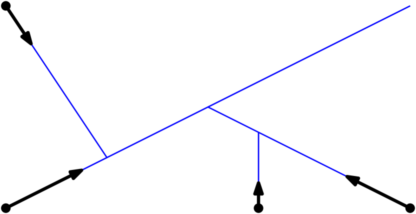
(a) A motorcycle graph

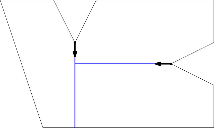
(b) Induced motorcycle graph

Figure 2: The motorcycle graph of a set of four motorcycles (a), and the motorcycle graph induced by the polygon from Figure 1.

The motorcycle graph is a special case of the straight skeleton, where each motorcycle is modeled by a small and thin triangle. Conversely, a polygon induces a motorcycle graph, where each motorcycle starts at a reflex vertex and moves with the same velocity as this vertex moves during the shrinking process. (See Figure 2b.) Cheng and Vigneron [15] showed that computing the straight skeleton of a non-degenerate polygon reduces to computing this induced motorcycle graph, and a lower envelope computation; Huber and Held extended this proof to degenerate cases [25]. The lower envelope computation can be done in $O(n\sqrt{h+1}\log^{2}n)$ expected time if $P$ has $h$ holes.

Previously, the bottleneck of straight skeleton computation was the induced motorcycle graph computation. This is our main motivation for designing a faster motorcycle graph algorithm. In this paper, we give an algorithm for computing a motorcycle graph that runs in $O(n^{4/3+\varepsilon})$ time, for any $\varepsilon>0$, improving on all previously known algorithms. Here is a brief description of our algorithm. For each motorcycle, we maintain a tentative track, which may be longer than its actual track in the motorcycle graph. We also maintain a set of target points, which contains the endpoints of the tentative tracks that have been created earlier for this motorcycle, and that it has not reached yet. Initially, the tentative tracks are empty, and then we try to extend them one by one, all the way to the destination point. If two tentative tracks cross, we retract them, by roughly halving the number of possible crossing points on each of them. After performing this halving, the tentative tracks do not intersect, and we can safely move the motorcycle that reaches the end of its tentative track first. Then we try to extend the tentative track of this motorcycle to its next target point, and repeat the process. An example is given in Appendix B.

Apart from obtaining better time bounds for straight skeleton computation, there are at least two other reasons for studying motorcycle graphs. First, Huber and Held [25] used the idea of computing the straight skeleton from its induced motorcycle graph to design and implement a practical straight skeleton algorithm. So it is important, even in practice, to get a better understanding of motorcycle graph computation. Another motivation for studying motorcycle graphs is a direct application to computer graphics, for quad mesh partitioning [19].

Some of our results make no particular assumptions on the input, but we also present a few results where we assume that the input coordinates are $O(\log n)$-bit rational numbers. We believe that this assumption is sufficient for most applications. For instance, in the applications mentioned above, it is hard to imagine that the input polygons would have features smaller than 1nm, and size larger than 1000km, so 64-bit integers should be more than sufficient.

1.1 Summary of our results and comparison with previous work

The main novelty in this paper is our algorithm for computing motorcycle graphs (Section 2.1). This algorithm is essentially different from the two previous algorithms [15, 18] that both simulate the construction in chronological order. Our algorithm, on the other hand, does not construct the motorcycle tracks in chronological order: It may move some motorcycle to its position at time $t$, and then later during the execution of the algorithm, move another motorcycle to its position at an earlier time $t^{\prime}<t$. (We give one such example in Appendix B.) This answers an open question by Eppstein and Erickson [18, end of Section 5], who asked whether the running time can be improved by relaxing the chronology of the events.

Our algorithm uses two auxiliary data structures, one for ray shooting, and another for halving queries. Given a query segment on the supporting line of a motorcycle, a halving query returns a splitting point on this segment such that there are roughly the same number of intersections with other supporting lines on both sides. (See Section 1.2.) The implementation of these data structures in different settings lead to different time bounds.

For all our results, we use the standard real-RAM model [31], that allows to perform arithmetic operations exactly on arbitrary real numbers. But for some of our results, we make the assumption that all input coordinates are $O(\log n)$-bit rational numbers. It has two advantages: It yields better time bounds, and allows us to handle the straight skeleton of degenerate polygons. This improvement comes from the fact that, for bounded precision input, two distinct crossing points between the supporting lines of two pairs of motorcycles are at distance $2^{-O(\log n)}$ from each other. It allows us to use a simpler halving scheme: Instead of halving a segment according to the number of intersection points, we use the midpoint according to the Euclidean distance. (See Section 3.3 and 4.1.)

Arbitrary precision input.

For our first set of results, the input coordinates are arbitrary real numbers, on which we can perform exact arithmetic operations. In this case, our new algorithm computes a motorcycle graph in $O(n^{4/3+\varepsilon})$ time (Theorem 5). This improves on the two subquadratic algorithms that were known before: the $O(n^{17/11+\varepsilon})$-time algorithm by Eppstein and Erickson [18], which was first published in 1998, and the $O(n^{3/2}\log n)$-time algorithm by Cheng and Vigneron [15], which first appeared in 2002.

We also give, in Section 3.2, an $O(Cn\log^{2}(n)\min(C,\log n))$-time algorithm for the case of $C$-oriented motorcycles, where the velocities take only $C$ different directions. This improves on the algorithm by Eppstein and Erickson [18], which runs in $O(n^{4/3+\varepsilon})$ time when $C=O(1)$.

Our last result with arbitrary precision input is an $O(n^{4/3+\varepsilon}+n\sqrt{h+1}\log^{2}n)$ expected time algorithm for computing the straight skeleton of a polygon with $n$ vertices and $h$ holes. (This result does not hold for a degenerate polygon where two reflex vertices may collide during the shrinking process, as in Figure 3.)

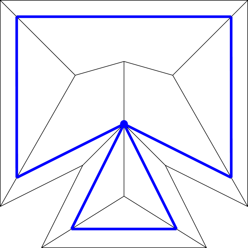
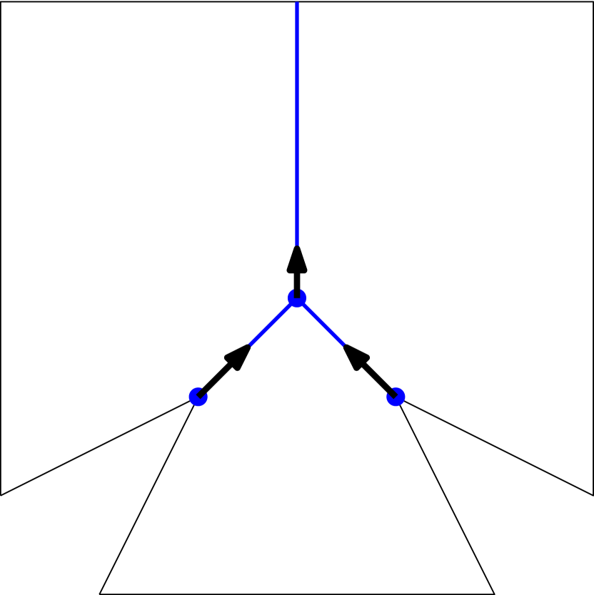
Figure 3: A degenerate polygon and its straight skeleton (left). Two reflex vertices collide during the shrinking process, and a new reflex vertex appears (middle). The induced motorcycle graph, where a new motorcycle appears when the two other crash (right).

It improves on the algorithm by Cheng and Vigneron [15] which runs in $O(n^{3/2}\log(n)+n\sqrt{h+1}\log^{2}n)$ expected time. It also improves on the $O(n^{17/11+\varepsilon})$ time bound of the algorithm by Eppstein and Erickson [18], but their algorithm is deterministic and applies to degenerate cases.

Bounded precision input.

The following results hold when all input coordinates are $O(\log n)$-bit rational numbers. There has been recent interest in studying computational geometry problems under a bounded precision model (the word RAM), for instance the computation of Delaunay triangulations, convex hulls, polygon triangulation and line segment intersections [8, 12].

We first show in Section 3.3 that a motorcycle graph can be computed in $O(n\log^{3}n)$ time if the motorcycles move within a simple polygon, starting from its boundary. The only other non-trivial cases where we know how to compute a motorcycle graph in near-linear time seem to be the case where all velocities have positive $x$-coordinate, which can be solved in $O(n\log n)$ time by plane sweep, the case of a constant number of different velocity vectors [18], or a constant number of directions (Section 3.2).

Then in Section 4.2, we show that the straight skeleton of a polygon with $n$ vertices and $h$ holes can be computed in $O(n\sqrt{h+1}\log^{3}n)$ expected time. This result still holds in degenerate cases. So with bounded-precision input, and if we allow randomization, it improves on the $O(n^{17/11+\varepsilon})$-time algorithm by Eppstein and Erickson [18]. When $h=o(n/\log^{2}n)$, it also improves on the $O(n^{3/2}\log^{2}n)$-time algorithm by Cheng and Vigneron [15], which cannot handle all degenerate cases.

In particular, our algorithm runs in expected $O(n\log^{3}n)$ time when $h=0$, so it is the first near-linear time algorithm for computing the straight skeleton of a simple polygon. The previously best known algorithms run in $\omega(n^{3/2})$ time in the worst case [15, 18].

1.2 Notation and preliminaries

For any two points $p,q$, we denote by $\overline{pq}$ the line segment between $p$ and $q$. Unless specified otherwise, $\overline{pq}$ is a closed segment. The relative interior of $\overline{pq}$ is the open segment $\overline{pq}\setminus\{p,q\}$. We say that two segments cross if their relative interiors intersect.

The motorcycles are numbered from $1$ to $n$. Each motorcycle $i$ has a starting point $s_{i}$, moves with constant velocity $\vec{v}_{i}$, and has a destination point $d_{i}$ that lies in the ray $(s_{i},\vec{v}_{i})$. (See Figure 4a.)

(a) Input

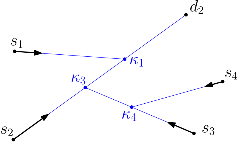
(b) Motorcycle graph

Figure 4: The input to the motorcycle graph problem (a), and the resulting motorcycle graph (b).

When $p\in\overline{s_{i}d_{i}}$, we denote by $\tau(i,p)$ the time when motorcycle $i$ reaches $p$, so $p=s_{i}+\tau(i,p)\vec{v_{i}}$. The supporting line $\ell_{i}$ of motorcycle $i$ is the line through $s_{i}$ with direction $\vec{v}_{i}$.

Each motorcycle $i$ starts at $s_{i}$ at time 0, and moves at velocity $\vec{v}_{i}$ until it meets the track left by another motorcycle and crashes, or it reaches $d_{i}$ and stops. So motorcycle $i$ crashes if it reaches a point $p$ such that $\tau(i,p)\geqslant\tau(j,p)$, for some motorcycle $j$ that has not crashed or stopped earlier than $\tau(j,p)$. If motorcycle $i$ crashes, we denote by $\kappa_{i}$ the point where it crashes, called the crashing point. (See Figure 4b.) Otherwise, $i$ reaches $d_{i}$, and we set $\kappa_{i}=d_{i}$. The trajectory of $i$ is the segment $\overline{s_{i}\kappa_{i}}$; in other words it is the track of $i$ in the motorcycle graph.

In the original motorcycle graph problem, the destination point $d_{i}$ is at infinity in direction $\vec{v}_{i}$. We can handle this case by computing a bounding box that includes all the vertices of the arrangement of the supporting lines $\ell_{i}$, $i=1,\dots,n$, and choosing as destination points the intersections of the rays $(s_{i},\vec{v}_{i})$ with the bounding box. The bounding box can be computed in $O(n\log n)$ time as any extreme vertex in the arrangement is the intersection of two lines with consecutive slopes.

Unless specified otherwise, we make the following general position assumptions. No two motorcycles share the same supporting line, or have parallel supporting lines. No three supporting lines are concurrent. No point $s_{i},d_{i}$ lies on $\ell_{j}$ if $j\neq i$. No two motorcycles reach the same point at the same time. (We make these assumptions so as to simplify the description of the algorithm and the proofs, but our results still hold in degenerate cases.)

The crossing point $\chi_{ij}$ is the intersection between $\ell_{i}$ and $\ell_{j}$, and thus $\chi_{ij}=\chi_{ji}=\ell_{i}\cap\ell_{j}$. The size $|pq|$ of a segment $\overline{pq}$ is the number of crossing points $\chi_{ij}$ that lie in $\overline{pq}$. (See Figure 5.)

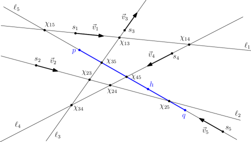
Figure 5: The size of $\overline{pq}$ is $|pq|=3$. Point $h$ is a possible result $h(p,q)$ of a halving query $(5,p,q)$ with $\rho=1/2$.

We will need a data structure to answer halving queries: Given a query $(i,p,q)$ where $p,q$ are points on the supporting line $\ell_{i}$, find a point $h=h(p,q)\in\overline{pq}$ such that $|ph|\leqslant\lceil\rho|pq|\rceil$ and $|hq|\leqslant\lceil\rho|pq|\rceil$, for a constant $\rho<1$. In addition, we require that $h$ is not a crossing point, and that both $|ph|$ and $|hq|$ are strictly smaller than $|pq|$ if $|pq|\geqslant 2$.

2 Algorithm for Computing Motorcycle Graphs

In this section, we present our algorithm for computing motorcycle graphs, as well as its proof of correctness and analysis. An example of the execution of this algorithm on a set of 4 motorcycles is given in Appendix B.

2.1 Algorithm description

Our algorithm maintains, for each motorcycle $i$, a confirmed track $\overline{s_{i}c_{i}}$, and a tentative track $\overline{s_{i}t_{i}}$, such that $c_{i}\in\overline{s_{i}d_{i}}$ and $t_{i}\in\overline{c_{i}d_{i}}$. So the tentative track is at least as long as the confirmed track. As we will show in the next section, the confirmed track is a subset of the trajectory, so we have $c_{i}\in\overline{s_{i}\kappa_{i}}$ at any time during the execution of the algorithm. The tentative track, however, may go beyond $\kappa_{i}$. (See Appendix B.)

Our algorithm will ensure that no two tentative tracks cross. We keep all the tentative tracks in a ray shooting data structure, so that we can enforce this invariant by checking for intersection each time we try to extend a tentative track. This data structure returns the first tentative track hit by a query ray $(p,\vec{v})$, if any. We also build a data structure to answer halving queries, which will be used to shorten tentative tracks and keep them disjoint.

Our algorithm builds the motorcycle graph by extending the confirmed tracks until they form the whole motorcycle graph. We may also update the tentative track of a motorcycle when we extend its confirmed track.

A set of target points is associated with each motorcycle $i$. In particular, we maintain in a stack $S_{i}$ the set of target points that lie beyond the confirmed track of motorcycle $i$, thus $S_{i}\subset\overline{c_{i}d_{i}}\setminus\{c_{i}\}$. In other words, $S_{i}$ records the target points that motorcycle $i$ has not reached yet. (See Figure 6.)

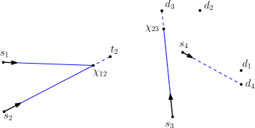
Figure 6: This is the same example as Appendix B, Figure (m). The confirmed tracks are solid, and the tentative tracks are dashed. For motorcycle 1, the confirmed track and the tentative track go to $\chi_{12}=c_{1}=t_{1}=\kappa_{1}$. The stack $S_{1}$ only records $d_{1}$. For motorcycle 2, the confirmed track ends at $c_{2}=\chi_{12}$, the tentative track ends at $t_{2}$, and $S_{2}=(t_{2},\chi_{23},d_{2})$. For motorcycle 3, we have $c_{3}=\chi_{23}$, $t_{3}=d_{3}$, and $S_{3}=(d_{3})$. For motorcycle 4, we have $c_{4}=s_{4}$, $t_{4}=d_{4}$, and $S_{4}=(d_{4})$.

The stack $S_{i}$ is ordered from $c_{i}$ to $d_{i}$. We denote by $\operatorname{Top}(S_{i})$ its first element, so $\operatorname{Top}(S_{i})$ is the target point in $S_{i}$ that is closest to $c_{i}$. At the beginning, we set $S_{i}=\{s_{i},d_{i}\}$ for all $i$. New target points will be created in Case (3b) of our algorithm, as described below.

If motorcycle $i$ has neither crashed nor stopped, then its tentative track ends at the first target point in $S_{i}$, so $t_{i}=\operatorname{Top}(S_{i})$. Otherwise, the tentative track and the confirmed track are the same, thus $t_{i}=c_{i}$. So after a motorcycle has crashed or stopped, the ray shooting data structure records its confirmed track.

An event $(i,p)$ happens when a motorcycle $i$ reaches a target point $p$. We process events one by one, and while an event is being processed, new events may be generated. After an event has been processed, we process the earliest available event. As $t_{i}=\operatorname{Top}(S_{i})$ is the closest target point to $i$ in $S_{i}$, it means that we always process the event $(i,t_{i})$ such that $\tau(i,t_{i})$ is smallest. Note that it does not imply that our simulation is done in chronological order: When we process an event $(i,t_{i})$, we may create a new event $(j,p)$ such that $\tau(j,p)<\tau(i,t_{i})$. (See Appendix B.)

We record in a priority queue $\mathcal{Q}$ the event $(i,t_{i})$ for each motorcycle $i$ that has not crashed or stopped. An event with earlier time $\tau(i,t_{i})$ has higher priority. As $t_{i}=\operatorname{Top}(S_{i})$, we can update the event queue $\mathcal{Q}$ in $O(\log n)$ time each time a stack $S_{i}$ is updated. So we can find the next available event in $O(\log n)$ time. The first $n$ events are the events $(i,s_{i})$, $i=1,\dots,n$, and occur at time $t=0$. We process these $n$ events in an arbitrary order.

We now explain how to process an event $(i,t_{i})$. To avoid confusion, for any motorcycle $j$, we use the notation $c_{j},t_{j}$ to denote the endpoints of its confirmed and tentative track just before processing this event, and we use the notation $c^{\prime}_{j},t^{\prime}_{j}$ for their position just after processing this event. We first extend the confirmed track of motorcycle $i$ to $t_{i}$, thus $c^{\prime}_{i}=t_{i}$. We also delete $t_{i}$ from $S_{i}$. We are now in one of the following cases:

• If $t_{i}=d_{i}$, then motorcycle $i$ stops. In order to avoid processing irrelevant events in the future, we remove $S_{i}$ from $\mathcal{Q}$.

• If $t_{i}$ is a crossing point $\chi_{ij}$ that lies in the confirmed track of $j$ (that is, $t_{i}\in\overline{s_{j}c_{j}}$), then $i$ crashes at $t_{i}$. So we remove $S_{i}$ from $\mathcal{Q}$.

• Otherwise, we try to extend the tentative track to the next target point $q=\operatorname{Top}(S_{i})$. So we perform a ray shooting query with ray $(t_{i},\vec{v}_{i})$, which gives us the first track intersected by $\overline{t_{i}q}$, if any.

  • If $\overline{t_{i}q}$ does not cross any track, then $t^{\prime}_{i}=q$, and we do not need to do anything else to handle this event.

  • Otherwise, let $j$ be the result of the ray-shooting query, so $\overline{s_{j}t_{j}}$ is the first track hit by segment $\overline{t_{i}q}$, starting from $t_{i}$. We shorten the tentative track of $i$, which means that we insert the new target point $\chi_{ij}$ into $S_{i}$, as well as the point $t^{\prime}_{i}=h(t_{i},\chi_{ij})$ obtained by a halving query on $\overline{t_{i}\chi_{ij}}$. If the crossing point $\chi_{ij}$ does not lie in the confirmed track of $j$, that is, if $\chi_{ij}\in\overline{c_{j}t_{j}}\setminus\{c_{j}\}$, then we also shorten the tentative track of $j$, so we insert $\chi_{ij}$ into $S_{j}$, and we insert $t^{\prime}_{j}=h(c_{j},\chi_{ij})$ into $S_{j}$.

After applying the rules above, we update the ray shooting data structure (if needed), and we move to the next available event.

2.2 Proof of correctness

Initially, we create the target points $s_{i},d_{i}$ for $i=1,\dots,n$. After this, we create new target points only in Case (3b) of our algorithm. There are two types of such target points: the crossing points $\chi_{ij}$ obtained by ray-shooting, and the points obtained by halving queries. We call $\chi$-targets the first type of target points, and $h$-targets the latter. By our assumption that the result of a halving query is not a crossing point, a target point cannot be both a $h$-target and a $\chi$-target.

We need the following lemma. Remember that we say that two segments cross if their relative interiors intersect.

Lemma 1.

During the course of the algorithm, no two tentative tracks cross.

Proof.

For sake of contradiction, assume that two tentative tracks cross during the course of the algorithm. Let $(i,t_{i})$ be the first event that generates such a crossing, so just before processing this event, the tentative tracks $\overline{s_{j}t_{j}}$, $j=1,\dots,n$ do not cross, and there is a crossing among the tracks $\overline{s_{j}t^{\prime}_{j}}$. We must be in Case (3), because we do not extend any tentative track in cases (1) and (2). Besides, we only extend the track of motorcycle $i$ in Case (3). So there must be another motorcycle $k\neq i$ such that $\overline{s_{i}t^{\prime}_{i}}$ crosses $\overline{s_{k}t_{k}}$.

In Case (3a), the segment $\overline{t_{i}q}$ obtained by ray shooting does not cross any tentative track $\overline{s_{j}t_{j}}$, $j\neq i$, and since $t^{\prime}_{i}=q$, then the new portion $\overline{t_{i}t^{\prime}_{i}}$ of the track does not cross any other tentative track. The same is true in Case (3b), because $t^{\prime}_{i}$ is in $\overline{t_{i}\chi_{ij}}$, where track $j$ is the first track hit by $\overline{t_{i}q}$. So we just proved that, in any case, the new portion $\overline{t_{i}t^{\prime}_{i}}$ of the track does not cross any track $\overline{s_{j}t_{j}}$, $j\neq i$, and in particular, $\overline{t_{i}t^{\prime}_{i}}$ does not cross $\overline{s_{k}t_{k}}$.

By our assumption, we also know that $\overline{s_{k}t_{k}}$ cannot cross $\overline{s_{i}t_{i}}$. So the only remaining possibility is that $\overline{s_{k}t_{k}}$ crosses $\overline{s_{i}t_{i}^{\prime}}$ at $t_{i}$. Then $t_{i}$ is the crossing point $\chi_{ik}$. This point $t_{i}=\chi_{ik}$ cannot be in the confirmed track $\overline{s_{k}c_{k}}$, because that would be Case (2) of our algorithm, and we showed that we are in Case (3). Since $\chi_{ik}$ is a $\chi$-target of $i$, and it does not lie in the confirmed track of $k$, then it must have been inserted at the same time in $S_{i}$ and $S_{k}$ while processing a previous event. Since $\chi_{ik}$ is not on the confirmed track of $k$, then it must still be in $S_{k}$. So the tentative track $\overline{s_{k}t_{k}}$ cannot contain $\chi_{ik}$ in its relative interior, a contradiction. ∎

We want to argue that our algorithm computes the motorcycle graph correctly. So assume it is not the case. As our algorithm moves motorcycles forward until they either reach their destination point or crash, it could only fail if during the execution of our algorithm, the confirmed track of at least one motorcycle $i$ goes beyond the point $\kappa_{i}$ where it is supposed to crash in the motorcycle graph. Let us consider the event $(i,t_{i})$ that is first processed by our algorithm, such that motorcycle $i$ goes beyond $\kappa_{i}$. So $\kappa_{i}$ is in the segment $\overline{c_{i}t_{i}}\setminus\{t_{i}\}$. Let $j$ denote the motorcycle that $i$ crashes into, in the (correct) motorcycle graph, so $\kappa_{i}=\chi_{ij}$.

When we process $(i,t_{i})$, in the current graph constructed by our algorithm, motorcycle $j$ cannot have reached $d_{j}$, because it would mean that the tentative tracks $\overline{s_{i}t_{i}}$ and $\overline{s_{j}d_{j}}$ are crossing at $\kappa_{i}=\chi_{ij}$, which is impossible by Lemma 1.

We now rule out the case where, when our algorithm processes $(i,t_{i})$, motorcycle $j$ has already crashed into some motorcycle $k$ in the graph constructed by the algorithm. (See Figure 7.) For sake of contradiction, assume it did happen.

Figure 7: The motorcycle graph (left) and an incorrect computation (right).

• If we had $i=k$, then $\chi_{ij}$ would have been created as a $\chi$-target for $j$ earlier. At this point, $i$ had not gone past $\chi_{ij}$, because $(i,t_{i})$ is the first such event. As $\tau(j,\chi_{ij})<\tau(i,\chi_{ij})$, the algorithm would have moved $j$ to $\chi_{ij}$ before $i$ moves further, and thus $j$ would not crash at $\chi_{ij}$, a contradiction.

• Thus we must have $i\neq k$. As $t_{i}$ is beyond $\kappa_{i}=\chi_{ij}$, and tentative tracks cannot cross, we must have $c_{j}\in\overline{s_{j}\chi_{ij}}$. So $j$ crashed into $k$ at $\chi_{jk}\in\overline{s_{j}\chi_{ij}}$. As in the correct motorcycle graph, $j$ does not crash into $k$, it means that the algorithm has already moved $k$ past its (correct) crashing point, which contradicts our assumption that $(i,t_{i})$ was the first such event.

We just proved that $j$ has not stopped or crashed when the algorithm processes event $(i,t_{i})$, so at this point there should be an event $(j,t_{j})$ in the queue. By Lemma 1, the tracks $\overline{s_{i}t_{i}}$ and $\overline{s_{j}t_{j}}$ cannot cross, so we must have $t_{j}\in\overline{c_{j}\kappa_{i}}$. (See Figure 8.)

Figure 8: Proof of correctness, remaining case.

It implies that $\tau(j,t_{j})\leqslant\tau(j,\kappa_{i})$. But since $i$ crashes into $j$ in the (correct) motorcycle graph, we must have $\tau(j,\kappa_{i})<\tau(i,\kappa_{i})$, thus $\tau(j,t_{j})<\tau(i,\kappa_{i})$. As $\kappa_{i}\in\overline{c_{i}t_{i}}$, we have $\tau(i,\kappa_{i})\leqslant\tau(i,t_{i})$, thus $\tau(j,t_{j})<\tau(i,t_{i})$. But this is impossible, because our algorithm always processes the earliest available event, so it would have processed $(j,t_{j})$ rather than $(i,t_{i})$.

2.3 Analysis

Our algorithm uses two auxiliary data structures: for answering halving queries, and for ray shooting. The running time of our algorithm depends on their preprocessing time and query time. Let $P(n)$ denote an upper bound on the preprocessing time of these two data structures, and let $Q(n)$ denote an upper bound on the time needed for a query or update—so we can answer a ray-shooting query or a halving query in time $Q(n)$, and we can update the ray shooting data structure in time $Q(n)$. We now prove the following result:

Theorem 2.

We can compute a motorcycle graph of size $n$ in time $O(P(n)+n(Q(n)+\log n)\log n)$.

Each time we handle an event, we perform at most two halving queries, one ray-shooting query, and we may update two tentative tracks in the ray-shooting data structure. We also pay an $O(\log n)$ time overhead to update the priority queue $\mathcal{Q}$. So after preprocessing, the running time will be at most the number of events times $Q(n)+\log n$. Thus we only need to argue that our algorithm processes a total of $O(n\log n)$ events. In fact, at each event we process, a motorcycle reaches a target point, so we only need to show that $O(n\log n)$ target points are created during the course of the algorithm.

Initially, we create $O(n)$ target points, which are $s_{i},d_{i}$ for $i=1,\dots,n$. After this, we only create new target points in Case (3b) of the algorithm. In this case, we create one $\chi$-target, and at most two $h$-targets obtained by halving. Thus we only need to bound the number of $\chi$-targets. At the end of the algorithm, some of these $\chi$-targets $\chi_{ij}$ correspond to an actual crash, with motorcycle $i$ crashing into $j$, or $j$ crashing into $i$. In any case, there are at most $n$ such $\chi$-targets. We need to consider the other $\chi$-targets, that do not correspond to an actual crash. In this case, either motorcycle $i$ or $j$ does not reach $\chi_{ij}$, so at the end of the computation, $\chi_{ij}$ must appear in the stack $S_{i}$ or $S_{j}$ of target points that have not been reached by motorcycle $i$ or $j$, respectively. Thus, in order to complete the proof of Theorem 2, we only need the following lemma.

Lemma 3.

At the end of the execution of our algorithm, for any motorcycle $i$, the number of $\chi$-targets in $S_{i}$ is $O(\log n)$.

Proof.

In this proof, we only consider the status of the stack $S_{i}$ at the end of the algorithm, and we assume that it contains more than one $\chi$-target. We denote by $\chi_{1},\dots,\chi_{m}$ the $\chi$-targets in $S_{i}$, in reverse order, so $\chi_{m}\dots\chi_{2}\chi_{1}$ is a subsequence of $S_{i}$, where $\chi_{m}$ is closest to $\kappa_{i}$ and $\chi_{1}$ is closest to $d_{i}$.

Each target $\chi_{j}$ was created in case (3b) of our algorithm. At the same time, an $h$-target $h_{j}=h(g_{j},\chi_{j})$ was created by a halving query using another target point $g_{j}$. As the points $\chi_{j}$, $j=1,\dots,m$ are in $S_{i}$, motorcycle $i$ never reaches these points during the course of the algorithm, so $\chi_{1}$ and $h_{1}$ must have been created first, then $\chi_{2}$ and $h_{2}$ …and finally $\chi_{m}$ and $h_{m}$.

For any $2\leqslant j\leqslant m$, as $\chi_{j}$ is created after $\chi_{j-1}$, and these two points are created when motorcycle $i$ reaches $g_{j}$ and $g_{j-1}$, respectively, it implies that $g_{j-1}$ is in $\overline{s_{i}g_{j}}$. We also know that $\chi_{j-1}$ lies in $\overline{\chi_{j}d_{i}}$, because $\chi_{j-1}$ appears after $\chi_{j}$ in $S_{i}$. So $\overline{g_{j}\chi_{j}}$, $j=1,\dots,m$ is a sequence of nested segments, that is, we have $\overline{g_{j}\chi_{j}}\subset\overline{g_{j-1}\chi_{j-1}}$ for all $2\leqslant j\leqslant m$. More precisely:

• If $h_{j-1}$ is in $S_{i}$, then $\overline{g_{j}\chi_{j}}\subset\overline{g_{j-1}h_{j-1}}$, because $\chi_{j}$ is created after $h_{j-1}$, and motorcycle $i$ never reaches $h_{j-1}$. (See Figure 9.)

• If $h_{j-1}$ is not in $S_{i}$, then $\overline{g_{j}\chi_{j}}\subset\overline{h_{j-1}\chi_{j-1}}$. (See Figure 10.) It can be proved as follows. As $h_{j-1}$ is created at the same time as $\chi_{j-1}$, then $\chi_{j}$ is created after $h_{j-1}$. So $\chi_{j}$ must have been created after motorcycle $i$ reaches $h_{j-1}$, otherwise we would have $\chi_{j}\in\overline{s_{i}h_{j-1}}$, and since motorcycle $i$ reaches $h_{j-1}$ later, $\chi_{j}$ would not be in $S_{i}$. As $\chi_{j}$ is created after motorcycle $i$ reaches $h_{j-1}$, we must have $g_{j}\in\overline{h_{j-1}\chi_{j-1}}$.

Figure 9: Proof of Lemma 3, first case.

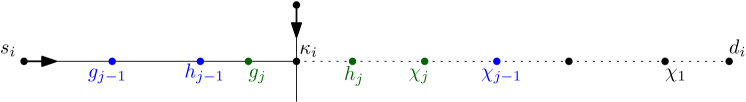
Figure 10: Proof of Lemma 3, second case.

Thus $\overline{g_{j}\chi_{j}}$ is contained in either $\overline{g_{j-1}h_{j-1}}$ or $\overline{h_{j-1}\chi_{j-1}}$, and since $h_{j-1}=h(g_{j-1},\chi_{j-1})$, it follows that the size $|g_{j}\chi_{j}|$ decreases exponentially when $j$ increases from 1 to $m$. As $\overline{g_{m-1}\chi_{m-1}}$ contains $\chi_{m}$ and $\chi_{m-1}$, we have $|g_{m-1}\chi_{m-1}|\geqslant 2$. In addition, $|g_{1}\chi_{1}|\leqslant n$, so we must have $m=O(\log n)$.

∎

3 Auxiliary Data Structures

Our algorithm, presented in Section 2.1, requires two auxiliary structures. The first one is simply a ray-shooting data structure. As ray shooting is a standard operation in computational geometry, we will be able to directly use known data structures. The second data structure we need is for answering halving queries. We show below how to construct efficient data structures for this type of queries, and the corresponding time bounds for our motorcycle graph algorithm.

3.1 General case

In this section, we present the auxiliary data structures for the most general case, as presented in Section 1.2. So motorcycles have arbitrary starting position, destination point and velocity.

For ray shooting, we can directly use a data structure by Agarwal and Matoušek [2], which requires preprocessing time $O(n^{4/3+\varepsilon})$, with update and query time $O(n^{1/3+\varepsilon})$, for any $\varepsilon>0$.

For halving queries, we use known range searching data structures and parametric search, as in the work of Agarwal and Matoušek on ray shooting: Our problem is an optimization version of range counting in an arrangement of lines, so we obtain the same bounds [2, Section 3.1].

Lemma 4.

Given the $n$ supporting lines $\ell_{1},\dots,\ell_{n}$, we can construct a data structure with $O(n^{4/3+\varepsilon})$ preprocessing time and $O(n^{1/3+\varepsilon})$ query time that answers the following queries $(i,p,q)$. Assume there are $k$ crossing points $\chi_{ij}$ on $\overline{pq}$. Then we return the median crossing point and the next: the $\lceil k/2\rceil$th and the $(\lceil k/2\rceil+1)$th such crossing point, in the ordering from $p$ to $q$ along $\overline{pq}$.

With the two auxiliary data structures above, Theorem 2 yields the following result.

Theorem 5.

A motorcycle graph can be computed in $O(n^{4/3+\varepsilon})$ time, for any $\varepsilon>0$.

It should be possible to replace the $n^{\varepsilon}$ factor in the bounds of Lemma 4 with a polylogarithm using known range searching techniques [11, 28], because we only need a static data structure for halving queries, but in any case we need a dynamic data structure for ray shooting queries, so it would not improve our overall time bounds.

3.2 $C$-Oriented Motorcycle Graphs

We consider the special case where motorcycles can only take $C$ different directions $\vec{d_{1}},\dots,\vec{d_{C}}$. Eppstein and Erickson gave an $O(n^{4/3+\varepsilon})$-time algorithm when $C=O(1)$. We show that with appropriate auxiliary data structures, we can solve this case in time $O(n\log^{3}n)$. In the following, we do not assume that $C=O(1)$, so our time bounds will also have a dependency on $C$.

Proposition 6.

We can compute a $C$-oriented motorcycle graph in $O(Cn\log^{2}(n)\min(C,\log n))$ time.

We use the following data structures, and then the result follows from Theorem 2.

Ray shooting data structures.

A first approach to answer our ray shooting queries is to use $C$ instances of a data structure for vertical ray shooting in a planar subdivision. Several data structures are known for this problem [6], we use a data structure by Cheng and Janardan [14] that takes $O(\log^{2}n)$ time per update and $O(\log n)$ time per query. So overall, we get $Q(n)=O(C\log^{2}n)$ with the terminology of Theorem 2.

Alternatively, we can use $C(C-1)$ instances of a data structure for vertical ray shooting among horizontal segments. Each data structure is used to answer ray shooting queries with a given direction, into segments with another direction: We just need to change the two coordinate axis to these two directions. Using a recent result by Giyora and Kaplan [22], we obtain $Q(n)=O(C^{2}\log n)$.

Halving queries.

Our data structure for halving queries simply consists of a sorted list of motorcycles for each direction. So for each $k\in 1,\dots,C$, we have an array $\mathcal{A}_{k}$ of the motorcycles with direction $\vec{d}_{k}$, sorted according to the intercept of their supporting lines with a line orthogonal to $\vec{d}_{k}$. We now explain how to answer a halving query $\overline{pq}\subset\ell_{i}$.

Without loss of generality, assume $\ell_{i}$ has direction $\vec{d}_{1}$. For each direction $\vec{d}_{k}$, $k=2,\dots,C$, the subset of motorcycles whose supporting lines cross $\overline{pq}$ appear in consecutive positions in $\mathcal{A}_{k}$. We can find the first and the last index of these lines in $O(\log n)$ time by binary search. So we obtain all the arrangement vertices in $\overline{pq}$ in $C-1$ sorted subarrays. We then compute the median $m_{k}$ of each such subarray $\mathcal{A}_{k}\cap\overline{pq}$, and the median of these points $m_{k}$ weighted by the number of points $|\mathcal{A}_{k}\cap\overline{pq}|$ in the corresponding subarray. This gives a halving point $h(p,q)$ with $\rho=3/4$. The median of each subarray can be found in $O(1)$ time, and their weighted median in $O(C)$ time [17], so the query time is dominated by the $C$ binary searches. Thus, we can answer halving queries in $O(C\log n)$ time.

3.3 Bounded precision input

The data structure for answering halving queries in Section 3.1 is quite involved. In practice, one would rather implement halving queries by simply halving the Euclidean length $\|pq\|$ instead of approximately halving the number of crossing points. Unfortunately, in the infinite precision model that is commonly used in computational geometry, this would cause the analysis of our algorithm in Lemma 3 to break down, because a stack of target points $S_{i}$ may have size $\Omega(n)$ at the end of the algorithm.

Such a counterexample would require the distance between consecutive target points in $S_{i}$ to become exponentially small near the crashing point, which does not seem likely to happen in practice. To formalize this idea, we make the assumption that all input numbers (the coordinates of the starting points, the destination points, and the velocities) are rational numbers, whose numerator and denominator are in $\{-2^{w-1},\dots,2^{w-1}-1\}$ for some integer $w$. In other words, the input numbers are $w$-bit signed integers. We still assume that arithmetic operations between two numbers can be performed in constant time.

This model also allows us to handle the case where input coordinates are $w$-bit rational numbers, that is, rational numbers with $w$-bit numerator and denominator; we just need to scale up each coordinate by a factor $2^{w}$ to obtain $2w$-bit integers, losing only a constant factor in our time bounds. In the proofs below we assume the input numbers are integers, to simplify the presentation, but the results are stated with rational coordinates.

As the input coordinates are $w$-bit integers, the coordinates of a crossing point $\chi_{ij}$ are rational numbers obtained by solving a $2\times 2$ linear system, their denominator being the determinant $\det(\vec{v}_{i},\vec{v}_{j})$. Thus, the denominator is an integer between $-2^{2w-1}$ and $2^{2w-1}$. So any two distinct crossing points are at distance at least $2^{-2w+1}$ from each other.

Assume that we replace our halving operation, as defined in Section 1.2, with halving the Euclidean length. So $h(p,q)$ is the midpoint of $\overline{pq}$, which can be computed in constant time. Then any nested sequence of segments obtained by successive halving, as in the proof of Lemma 3, consists of $O(w)$ such nested segments, because a segment $\overline{g_{j}\chi_{j}}$ of length smaller than $2^{-2w+1}$ cannot contain another crossing point in its interior, and hence it cannot be further subdivided. So the bound on the size of $S_{i}$ becomes $O(w)$, and we get the following result.

Theorem 7.

If the input coordinates are $w$-bit rational numbers, we can compute a motorcycle graph in time $O(nw(Q^{\prime}(n)+\log n))$, where $Q^{\prime}(n)$ is the time needed for updates or queries in the ray-shooting data structure.

For bounded-precision input, the bottleneck of our algorithm has thus become the ray shooting data structure, whose update and query time bound is $O(n^{1/3+\varepsilon})$ in the most general case. Therefore, we obtain a faster motorcycle graph algorithm if we are in a special case where faster ray-shooting data structures are known. One such case is ray-shooting in a connected planar subdivision, which can be done in $O(\log^{2}n)$-time per update and query using a data structure by Goodrich and Tamassia [23]. We can use this data structure if, for instance, all motorcycles move inside a simple polygon $P$, starting from its boundary. (So for all $i$, $\overline{s_{i}d_{i}}\subset P$, and $s_{i}$ is on the boundary of $P$.) Then we perform ray shooting in the union of the tentative tracks and the edges of $P$, which form a connected subdivision. It yields the following time bound.

Corollary 8.

We can compute a motorcycle graph in time $O(n\log^{3}n)$ for $n$ motorcycles moving inside a simple polygon with $O(n)$ vertices, starting on its boundary, and if the input has $O(\log n)$-bit rational coordinates.

4 Application to Straight Skeleton Computation

In this section, we give new results on straight skeleton computation, using our new motorcycle graph algorithm.

4.1 Preliminaries and non-degenerate cases

As we mentioned in the introduction, the straight skeleton problem and the motorcycle graph problem are closely related. We now explain it in more details.

Consider the reflex (non-convex) vertices of a polygon $P$. When we construct the straight skeleton of $P$, these vertices move inward and may collide into edges, or other vertices. These events, called split events and vertex events, are the difficult part of straight skeleton computation, because they affect the topology of the shrinking polygon by splitting it, and because they are non-local: A reflex vertex may affect a chain of edges on the other side of the polygon. The other type of events, called edge events, where an edge shrinks to a point, are easily handled with a priority queue. So the interaction between reflex vertices is a crucial part in straight skeleton computation, and the motorcycle graph presented below helps to determine these interactions.

The motorcycle graph induced by a polygon $P$ is such that each motorcycle starts at a reflex vertex, moves as the same velocity as the corresponding reflex vertex when we shrink $P$, and stops if it reaches the boundary $\partial P$ of $P$. (See Figure 2.)

If $P$ is degenerate, then two reflex vertices may collide and create a new reflex vertex. In this case we need to create a new motorcycle after the collision. (See Figure 3.) So when two motorcycles collide in the induced motorcycle graph, we may have to create a new motorcycle [25]. Our motorcycle graph algorithm, as described above, does not apply directly to this case, because the proof of Lemma 3 breaks down. (The reason is that $S_{i}$ may hold a linear number of target points at the end of the execution of the algorithm, due to the newly created motorcycles. See Figure 11.)

Figure 11: An example where $S_{i}$ holds a linear number of target points at the end of execution of the algorithm. The speed of the motorcycle at the bottom are adjusted so that $\chi_{1}$ is created first, then $\chi_{2}$…

In Section 4.2, we will explain how to compute these generalized motorcycle graphs efficiently on bounded-precision input. But the following theorem still holds in degenerate cases.

Theorem 9 (Cheng and Vigneron [15], Huber and Held [25]).

The straight skeleton of a polygon $P$ with $n$ vertices and $h$ holes can be computed in expected time $O(n\sqrt{h+1}\log^{2}n)$ if we know the motorcycle graph induced by the vertices of $P$.

From the discussion above, and using our motorcycle graph algorithm from Theorem 5, we obtain the following result.

Corollary 10.

We can compute the straight skeleton of a non-degenerate polygon with $n$ vertices and $h$ holes in $O(n^{4/3+\varepsilon}+n\sqrt{h+1}\log^{2}n)$ time for any $\varepsilon>0$.

4.2 Bounded precision input

We use the same bounded precision assumptions as in Section 3.3, where the input coordinates are $w$-bit integers or, equivalently, $w$-bit rational numbers. Similarly, to simplify the presentation, we use the integer model in the proofs, but we state the results in the rational model.

Thus, the coordinates of the vertices of the input polygon $P$ are $w$-bit integers. The supporting lines $\ell_{i}$ of the motorcycles are angle bisectors between two edges of the input polygon. In order to apply the same halving scheme as in Section 3.3, where the Euclidean length is used instead of the number of arrangement vertices, we need to argue that the separation between two vertices in this arrangement of bisectors cannot be too small. This distance can be shown to be at least $2^{-W}$, where $W=64(80w+105)+1=O(w)$, by applying the separation bound by Burnikel et al. [9]. So we obtain a result for induced motorcycle graphs that is analogous to Theorem 7.

Lemma 11.

Given a polygon $P$ whose input coordinates are $w$-bit rational numbers, we can compute the motorcycle graph induced by $P$ in time $O(nw(Q^{\prime}(n)+\log n))$, where $Q^{\prime}(n)$ is the time needed for updates or queries in the ray-shooting data structure.

In the lemma statement above, we do not exclude degenerate cases. This is another advantage of this bounded precision model. As the argument in our analysis only relies on the separation bound between two distinct crossing points, and not on the number of motorcycles crossing a given segment, a newly created motorcycle does not affect our analysis as it still obeys the same separation bound: A newly created motorcycle still lies on the bisector of two input edges, though these two edges are not adjacent in the input polygon [25]. (See Figure 3.)

We still need to describe an efficient ray-shooting data structure. As our input polygon has $h$ holes, the boundary $\partial P$ of $P$ together with the tentative tracks form a collection of $h+1$ disjoint simple polygons. We could directly use known ray-shooting data structures [4, 24], which can be made dynamic at the expense of an extra $n^{\varepsilon}$ factor in the running time [1]. In the following, we give a different approach, which leads to a better time bound when used as a subroutine of our algorithm. This approach takes advantage of the fact that the holes of $P$ are fixed (only the tentative tracks are dynamic). We use a spanning tree with low crossing number, which is not a new idea in ray-shooting data structures [13, 24].

We pick one point on the boundary of each hole of $P$, and on the boundary of $P$. We connect these $h+1$ points using a spanning tree $\mathcal{T}$ with low stabbing number [3], that is, a spanning tree such that any line crosses at most $O(\sqrt{h})$ edges of $T$. This tree can be computed in $O(n^{1+\varepsilon})$ time [3, Section 8]. We maintain a polygonal subdivision which is the overlay of $P$ with $\mathcal{T}$ and the tentative tracks. So at each intersection between an edge of $\mathcal{T}$ and an edge of $P$ or a tentative track, we split the corresponding edges and tracks at the intersection point. This subdivision $\mathcal{S}$ is connected and has $O(n\sqrt{h})$ edges, and we maintain it in the ray shooting data structure by Goodrich and Tamassia [23], which has $O(\log^{2}n)$ update and query time.

Each time a tentative track is extended or retracted, as a tentative track intersects $O(\sqrt{h})$ edge of $\mathcal{T}$, we can update the subdivision and the data structure by making $O(\sqrt{h})$ updates in the ray shooting data structure. Similarly, when our motorcycle graph algorithm tries to extend a tentative track, we can find the first tentative track being hit by a query ray in $O(\sqrt{h}\log^{2}n)$ time: We first perform a ray shooting query in $\mathcal{S}$, which takes $O(\log^{2}n)$ time. If we hit an edge of $\mathcal{T}$, we make another ray shooting query starting at the hitting point of the previous query, and in the same direction. We repeat this process as long as the result of the query is an edge of $\mathcal{T}$, and by the low-stabbing number property, it may only happen $O(\sqrt{h})$ times.

Overall, our ray shooting data structure has update and query time $O(\sqrt{h}\log^{2}n)$. So by Theorem 9 and Lemma 11, we obtain the following result. Note that it still holds for degenerate input.

Theorem 12.

The straight skeleton of a polygon with $n$ vertices and $h$ holes, whose coordinates are $O(\log n)$-bit rational numbers, can be computed in $O(n\sqrt{h+1}\log^{3}n)$ expected time.

Appendix

Appendix A Pseudocode

In this section, we give the pseudocode of our algorithm. It is more detailed than the algorithm description in Section 2.1, and it can handle degenerate cases. The proof of correctness and the analysis are essentially the same as in Section 2, but they require a more detailed case analysis.

To deal with the degenerate cases where some supporting lines are concurrent, or two or more motorcycles reach a point at the same time, we record all the target points created so far in a dictionary data structure $\mathcal{D}$. We can implement $\mathcal{D}$ as a balanced binary search tree, sorted in lexicographical order of the coordinates $(x,y)$, which allows to retrieve a point in $O(\log n)$ time. We associate three fields with each point $p$ stored in $\mathcal{D}$:

• A list $M(p)$ records the motorcycles $i$ such that $p\in S_{i}$. So $M(p)$ records all the motorcycles $i$ that could possibly reach $p$, at a given point of the execution of our algorithm. The set $M(p)$ itself is stored in a dictionary data structure, so that we can decide in $O(\log n)$ time whether a motorcycle $i$ is in $M(p)$.

• Two motorcycles $k,k^{\prime}$ of $M(p)$ such that $\tau(k,p),\tau(k^{\prime},p)$ are smallest. It will allow us to find out whether two motorcycles crash simultaneously at $p$.

• A flag $\operatorname{Blocked}(p)$ which is set to FALSE initially, and is set to TRUE as soon as a confirmed track has reached $p$, implying that any other motorcycle that reaches $p$ must crash.

After the initialization stage, our algorithm handles repeatedly the earliest available event, according to the four cases (1), (2), (3a) and (3b) from Section 2.1.

Lines 11 and 12 deal with Case (1) and (2). The condition $p=d_{i}$ corresponds to Case (1). The other two conditions check whether we are in Case (2). In particular, condition $\operatorname{Blocked}(p)=\mbox{TRUE}$ means that at least one other motorcycle has reached $p$, thus motorcycle $i$ crashes. With degenerate input, it is possible that another (or several other) motorcycle reaches $p$ at the same time as $i$, in which case $\operatorname{Blocked}(p)=\mbox{FALSE}$ if $(i,p)$ is the first event involving $p$ that has been processed. The condition at Line 12 checks whether we are in this situation. If so, $i$ must crash. As $(i,p)$ is the first event involving $p$ that we process, there is no earlier event in $M(p)$, so we can find another motorcycle that reaches $p$ at the same time in constant time using the second field associated with $p$ in $\mathcal{D}$.

Case (3a) corresponds to a positive answer to the test at Line 19. The condition $d(s_{i},p^{\prime})>d(s_{i},\operatorname{Top}(S_{i}))$ detects whether the track of $i$ to the next target points hits any other track. The other condition $p^{\prime}=\operatorname{Top}(S_{i})$ and $j\in M(p^{\prime})$, checks for a boundary case, where $\operatorname{Top}(S_{i})$ falls on another tentative track. The test is positive if $p^{\prime}$ has already been identified as a target point of $j$ before. In this case we only extend the tentative track of $i$, without doing any unnecessary halving.

Line 21 branches to Case (3b). Similar to Line 19, we do not perform an unnecessary halving operation when $i\in M(p^{\prime})$ or $j\in M(p^{\prime})$.

Our pseudocode does not handle explicitly the case where two motorcycles have same supporting line. These cases can be easily handled by ad-hoc arguments [15]. One way of doing it is to insert additional target points at initialization. For each supporting line shared by several motorcycles, between any two consecutive motorcycles $i,j$ along this line that go toward each other, we insert their potential collision point, that is, we insert into $S_{i}$ and $S_{j}$ the point $p$ such that $\tau(i,p)=\tau(j,p)$. For each motorcycle $i$ along this line, if the first starting point $s_{j}$ in the ray $(s_{i},\vec{v}_{i})$ is in $\overline{s_{i}d_{i}}$, we also update $d_{i}$ to be $s_{j}$.

Algorithm 1 motorcycle_graph

1:Initialize the dictionary $\mathcal{D}$. $\triangleright$ Initialization

2:for $i=1\to n$ do

3:     Set $c_{i}\leftarrow s_{i}$, $t_{i}\leftarrow s_{i}$ and $S_{i}\leftarrow\{s_{i},d_{i}\}$.

4:     Insert $s_{i}$ and $d_{i}$ into $\mathcal{D}$;

5:     Insert motorcycle $i$ into $M(s_{i})$ and $M(d_{i})$.

6:Initialize the event queue $Q$ and the data structures for ray-shooting and halving.

7:while ${Q}$ is not empty do $\triangleright$ Main loop

8:     Let $(i,p)$ be the earliest available event. $\triangleright$ So $p=t_{i}$.

9:     Set $c_{i}\leftarrow p$.

10:     Pop $\operatorname{Top}(S_{i})$ from $S_{i}$. $\triangleright$ Here $\operatorname{Top}(S_{i})=p$.

11:     if $\operatorname{Blocked}(p)=\mbox{TRUE}$, or $p=d_{i}$, or

12:         $\exists k\in M(p)\setminus\{i\}$ such that $\tau(k,p)=\tau(i,p)$ then

13:         Motorcycle $i$ crashes.

14:         Set $t_{i}\leftarrow p$.

15:         Remove $i$ from $M(j)$ for all $j\in S_{i}$.

16:         Remove $S_{i}$ from $Q$.

17:     else

18:         $(j,p^{\prime})\leftarrow\operatorname{rayshooting}(c_{i},\vec{v}_{i})$.

19:         if $d(s_{i},p^{\prime})>d(s_{i},\operatorname{Top}(S_{i}))$, or ($p^{\prime}=\operatorname{Top}(S_{i})$ and $j\in M(p^{\prime})$) then

20:              Set $t_{i}\leftarrow\operatorname{Top}(S_{i})$.

21:         else

22:              if $i\in M(p^{\prime})$ then

23:                  Set $t_{i}\leftarrow\operatorname{Top}(S_{i})$.

24:              else

25:                  Push $p^{\prime}$ into $S_{i}$.

26:                  Push $p^{*}=h(c_{i},p^{\prime})$ into $S_{i}$.

27:                  Set $t_{i}\leftarrow p^{*}$.

28:                  Insert $i$ into $M(p^{\prime})$ and $M(p^{*})$.               

29:              if $p^{\prime}\notin\overline{s_{j}c_{j}}$ and $j\notin M(p^{\prime})$ then

30:                  Push $p^{\prime}$ into $S_{j}$.

31:                  Push $p^{*}=h(c_{j},p^{\prime})$ into $S_{j}$.

32:                  Set $t_{j}\leftarrow p^{*}$.

33:                  Insert $j$ into $M(p^{\prime})$ and $M(p^{*})$.                             

34:     Set $\operatorname{Blocked}(p)\leftarrow\mbox{TRUE}$.

Appendix B Example

We give an example of the execution of our algorithm on a set of 4 motorcycles. (Confirmed tracks are solid, and tentative tracks are dotted.) It demonstrates two features of our algorithm, that were mentioned above.

• A tentative track may be longer than the final track in the motorcycle graph. For instance, the tentative track $\overline{s_{1}d_{1}}$ in (b) is longer than the final track $\overline{s_{1}\chi_{12}}$ in (q).

• Our algorithm does not construct the motorcycle graph in chronological order. For instance, in (i), motorcycle 2 is moved to $\chi_{12}$, which is its position at time $\tau(2,\chi_{12})=2.12072$. Then in (k), motorcycle 3 is moved to $p_{4}$, which is its position at time $\tau(3,p_{4})=1.667206$.

The four motorcycles $1,2,3$ and $4$ start at time $0$ at initial points $s_{1}=(0.8,3.3)$, $s_{2}=(0.5,1)$, $s_{3}=(5.7,0)$ and $s_{4}=(6,3.4)$. Their velocities are $v_{1}=1.2(\cos-5^{\circ},\sin-5^{\circ})$, $v_{2}=1.7(\cos 35^{\circ},\sin 35^{\circ})$, $v_{3}=2(\cos 93^{\circ},\sin 93^{\circ})$, and $v_{4}=0.8(\cos-37^{\circ},\sin-37^{\circ})$.

We use the halving scheme as specified in Section 1.2 with $\rho=1/2$. So for instance, we create $p_{4}$ in (j) by halving $\overline{s_{3}\chi_{23}}$. There are three crossings along this segment: $\chi_{13},\chi_{23},\chi_{34}$. Then $p_{4}$ is created as a point between $\chi_{13}$ and $\chi_{34}$, in this case we just use the midpoint.

(a)

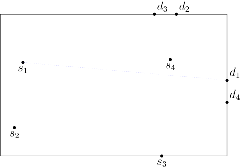
(b) $\tau(1,d_{1})=6.022919$

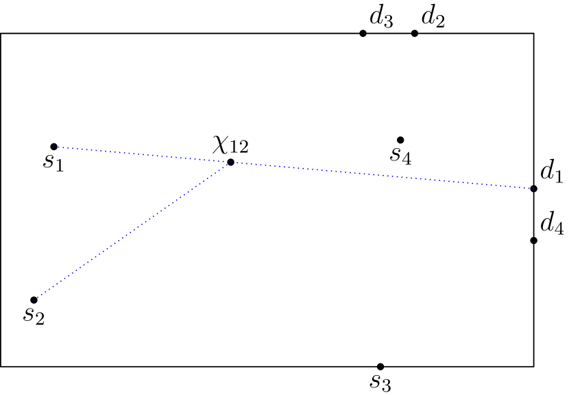
(c) new events: $\tau(1,\chi_{12})=2.219469$, and $\tau(2,\chi_{12})=2.120721$

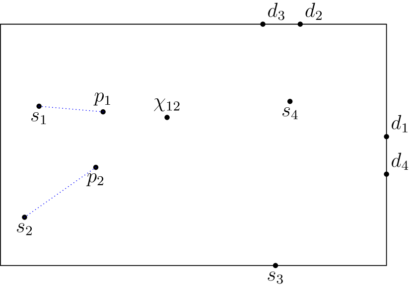
(d) new events: $\tau(1,p_{1})=1.109735$, and $\tau(2,p_{2})=1.060361$

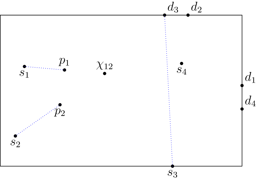
(a) $\tau(3,d_{3})=2.503431$

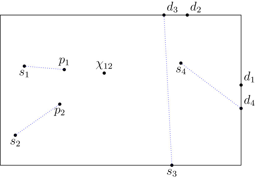
(b) $\tau(4,d_{4})=3.130339$

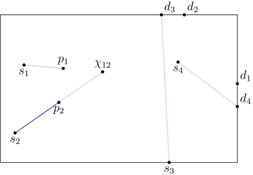
(c) move: $\tau(2,p_{2})=1.060361$

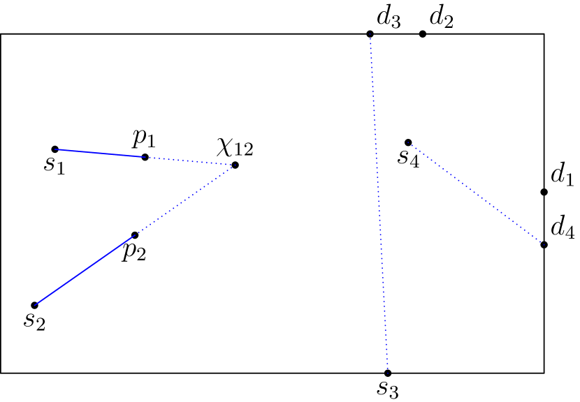
(d) move: $\tau(1,p_{1})=1.109735$

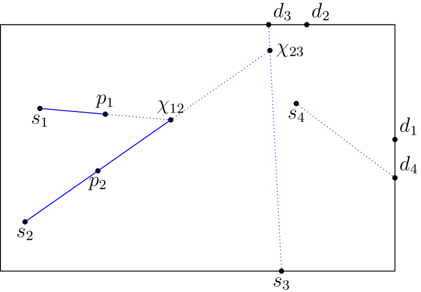
(e) move: $\tau(2,\chi_{12})=2.120721$. new events: $\tau(2,\chi_{23})=3.565653$, and $\tau(3,\chi_{23})=2.24147$

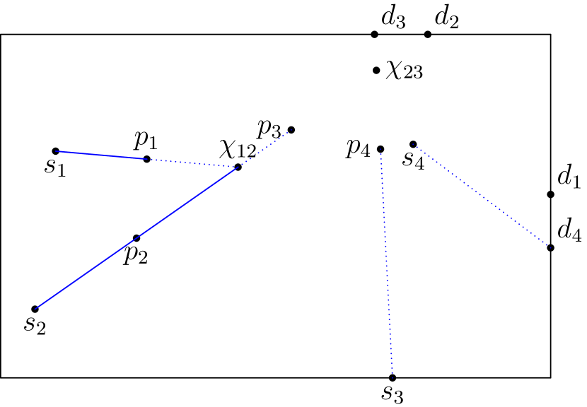
(f) new events: $\tau(2,p_{3})=2.676739$, and $\tau(3,p_{4})=1.667206$

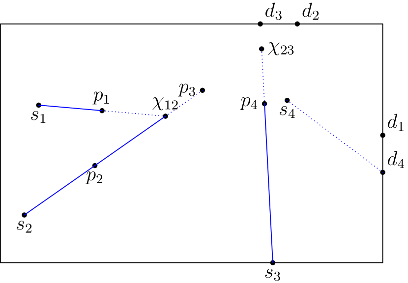
(a) move: $\tau(3,p_{4})=1.667206$

(b) move: $\tau(1,\chi_{12})=2.219469$

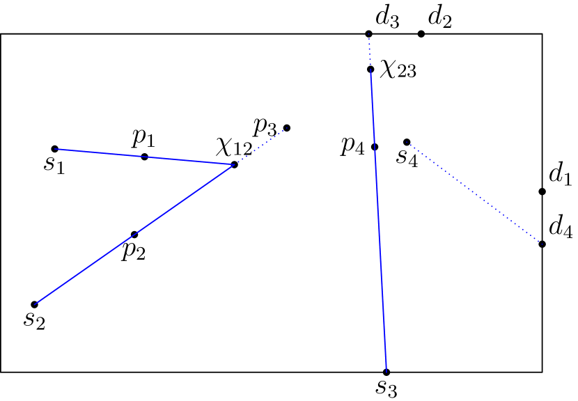
(c) move: $\tau(3,\chi_{23})=2.24147$

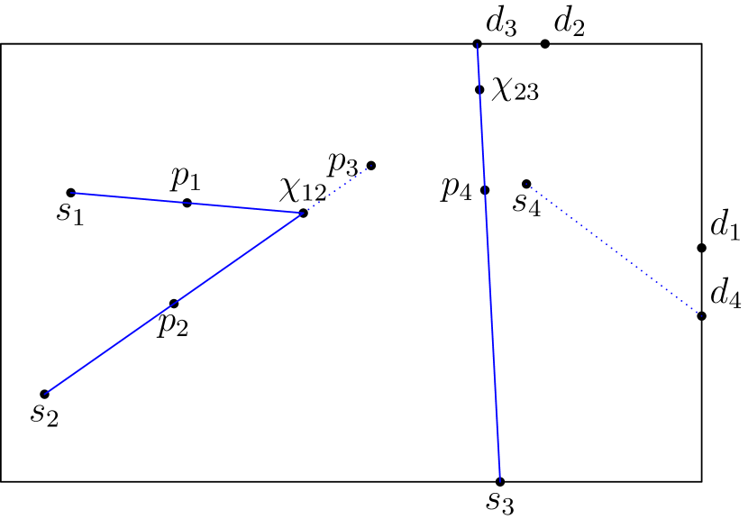
(d) move: $\tau(3,d_{3})=2.503431$

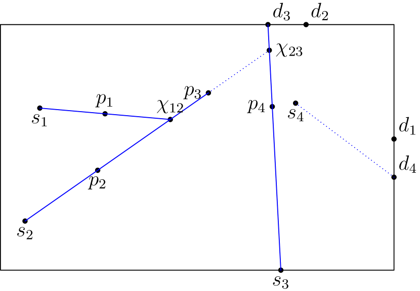
(e) move: $\tau(2,p_{3})=2.676739$

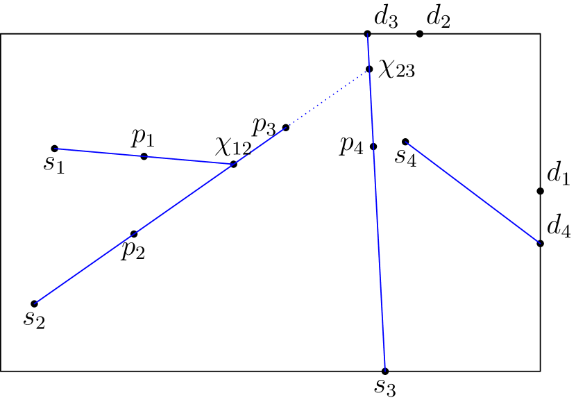
(f) move: $\tau(4,d_{4})=3.130339$

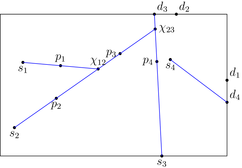
(g) move: $\tau(2,\chi_{23})=3.565653$

References

- [1] P. Agarwal and J. Erickson. Geometric range searching and its relatives. In B. Chazelle, J. E. Goodman, and R. Pollack, editors, Advances in Discrete and Computational Geometry, volume 23, page 1―56. American Mathematical Society, 1998.
- [2] P. Agarwal and J. Matoušek. Ray shooting and parametric search. SIAM Journal on Computing, 22(4):794–806, 1993.
- [3] P. Agarwal and M. Sharir. Applications of a new space-partitioning technique. Discrete & Computational Geometry, 9(1):11–38, 1993.
- [4] P. Agarwal and M. Sharir. Ray shooting amidst convex polygons in 2D. Journal of Algorithms, 21(3):508–519, 1996.
- [5] O. Aichholzer, F. Aurenhammer, D. Alberts, and B. Gärtner. A novel type of skeleton for polygons. Journal of Universal Computer Science, 1(12):752–761, 1995.
- [6] L. Arge, G. S. Brodal, and L. Georgiadis. Improved dynamic planar point location. In Proc. 47th Symposium on Foundations of Computer Science, pages 305–314, 2006.
- [7] G. Barequet, M. Goodrich, A. Levi-Steiner, and D. Steiner. Straight-skeleton based contour interpolation. In Proc. 14th ACM-SIAM Symposium on Discrete Algorithms, pages 119–127, 2003.
- [8] K. Buchin and W. Mulzer. Delaunay triangulations in o(sort(n)) time and more. Journal of the ACM, 58(2):6, 2011.
- [9] C. Burnikel, R.Fleischer, K. Mehlhorn, and S. Schirra. A strong and easily computable separation bound for arithmetic expressions involving square roots. In Proc. 8th ACM-SIAM Symposium on Discrete Algorithms, pages 702–709, 1997.
- [10] F. Cacciola. A cgal implementation of the straight skeleton of a simple 2d polygon with holes. In 2nd CGAL User Workshop, 2004. http://www.cgal.org/UserWorkshop/2004/straight_skeleton.pdf.
- [11] T. Chan. Optimal partition trees. Discrete & Computational Geometry, 47(4):661–690, 2012.
- [12] T. Chan and M. Patrascu. Transdichotomous results in computational geometry, i: Point location in sublogarithmic time. SIAM Journal on Computing, 39(2):703–729, 2009.
- [13] B. Chazelle, H. Edelsbrunner, M. Grigni, L. Guibas, J. Hershberger, M. Sharir, and J. Snoeyink. Ray shooting in polygons using geodesic triangulations. Algorithmica, 12(1):54–68, 1994.
- [14] S.-W. Cheng and R. Janardan. New results on dynamic planar point location. SIAM Journal on Computing, 21(5):972–999, 1992.
- [15] S.-W. Cheng and A. Vigneron. Motorcycle graphs and straight skeletons. Algorithmica, 47(2):159–182, 2007.
- [16] F. Cloppet, J. Oliva, and G. Stamon. Angular bisector network, a simplified generalized voronoi diagram: Application to processing complex intersections in biomedical images. IEEE Transactions on Pattern Analysis and Machine Intelligence, 22(1):120–128, 2000.
- [17] T. Cormen, C. Leiserson, R.Rivest, and C. Stein. Introduction to Algorithms. The MIT Press, 3 edition, 2009.
- [18] D. Eppstein and J. Erickson. Raising roofs, crashing cycles, and playing pool: Applications of a data structure for finding pairwise interactions. Discrete & Computational Geometry, 22(4):569–592, 1999.
- [19] D. Eppstein, M. Goodrich, E. Kim, and R. Tamstorf. Motorcycle graphs: Canonical quad mesh partitioning. Computer Graphics Forum, 27(5):1477–1486, 2008.
- [20] J. Erickson. Crashing motorcycles efficiently. http://www.cs.uiuc.edu/~jeffe/open/cycles.html, 1998.
- [21] P. Felkel and Š. Obdržálek. Straight skeleton implementation. In Proc. 14th Spring Conference on Computer Graphics, pages 210–218, 1998.
- [22] Y. Giyora and H. Kaplan. Optimal dynamic vertical ray shooting in rectilinear planar subdivisions. In Proc. 18th ACM-SIAM Symposium on Discrete Algorithms, pages 19–28, 2007.
- [23] M. Goodrich and R. Tamassia. Dynamic ray shooting and shortest paths in planar subdivisions via balanced geodesic triangulations. Journal of Algorithms, 23(1):51–73, 1997.
- [24] J. Hershberger and S. Suri. A pedestrian approach to ray shooting: Shoot a ray, take a walk. Journal of Algorithms, 18(3):403–431, 1995.
- [25] S. Huber and M. Held. Theoretical and practical results on straight skeletons of planar straight-line graphs. In Proc. 27th Symposium on Computational Geometry, pages 171–178, 2011.
- [26] T. Kelly and P. Wonka. Interactive architectural modeling with procedural extrusions. ACM Transactions on Graphics, 30(2):14:1–14:15, 2011.
- [27] R. Laycock and A. Day. Automatically generating large urban environments based on the footprint data of buildings. In Proc. 8th ACM symposium on Solid Modeling and Applications, pages 346–351, 2003.
- [28] J. Matoušek. Efficient partition trees. Discrete & Computational Geometry, 8:315–334, 1992.
- [29] J. Oliva, M. Perrin, and S. Coquillart. 3D reconstruction of complex polyhedral shapes from contours using a simplified generalized voronoi diagram. Computer Graphics Forum, 15(3):397–408, 1996.
- [30] P. Palfrader, M. Held, and S. Huber. On computing straight skeletons by means of kinetic triangulations. In Proc. 20th European Symposium on Algorithms, pages 766–777, 2012.
- [31] F. Preparata and M. Shamos. Computational Geometry: An Introduction. Springer, Berlin, 1985.
- [32] G. von Peschka. Kotirte Ebenen. Buschak & Irrgang, Brünn, 1877.