Finite element approximations of the stochastic mean curvature flow of planar curves of graphs

Abstract.

This paper develops and analyzes a semi-discrete and a fully discrete finite element method for a one-dimensional quasilinear parabolic stochastic partial differential equation (SPDE) which describes the stochastic mean curvature flow for planar curves of graphs. To circumvent the difficulty caused by the low spatial regularity of the SPDE solution, a regularization procedure is first proposed to approximate the SPDE, and an error estimate for the regularized problem is derived. A semi-discrete finite element method, and a space-time fully discrete method are then proposed to approximate the solution of the regularized SPDE problem. Strong convergence with rates are established for both, semi- and fully discrete methods. Computational experiments are provided to study the interplay of the geometric evolution and gradient type-noises.

1. Introduction

The mean curvature flow (MCF) refers to a one-parameter family of hypersurfaces $\{\Gamma_{t}\}_{t\geq 0}\subset\mathbf{R}^{d+1}$ which starts from a given initial surface $\Gamma_{0}$ and evolves according to the geometric law

$$V_{n}(t,\cdot)=H(t,\cdot),$$

where $V_{n}(t,\cdot)$ and $H(t,\cdot)$ denote respectively the normal velocity and the mean curvature of the hypersurface $\Gamma_{t}$ at time $t$. The MCF is the best known curvature-driven geometric flow which finds many applications in differential geometry, geometric measure theory, image processing and materials science and have been extensively studied both analytically and numerically (cf. [10, 16, 24, 29, 32] and the references therein).

As a geometric problem, the MCF can be described using different formulations. Among them, we mention the classical parametric formulation [18], Brakke’s varifold formulation [2], De Giorgi’s barrier function formulation [9, 3, 4], the variational formulation [1], the level set formulation [26, 14, 8], and the phase field formulation [13, 19]. We remark that different formulations often lead to different solution concepts and also lead to developing different analytical (and numerical) concepts and techniques to analyze and approximate the MCF. However, all these formulations of the MCF give rise to difficult but interesting nonlinear geometric partial differential equations (PDEs), and the resolution of the MCF then depends on the solutions of these nonlinear geometric PDEs. One interesting feature of the MCF is the development of singularities, in particular singularities which may occur in finite time, even when the initial hypersurface is smooth. The singularities may appear in different forms such as self-intersection, pinch-off, merging, and fattening. To understand and characterize these singularities have been the focus of the analytical and numerical research on the MCF (cf. [8, 10, 14, 15, 24, 29, 32], and the references therein).

For application problems, there is a great deal of interest to include stochastic effects, and to study the impact of special noises on regularities of solutions, as well as their long-time behaviors. The uncertainty may arise from various sources such as thermal fluctuation, impurities of the materials, and the intrinsic instabilities of the deterministic evolutions. In this paper we consider the following form of a stochastically perturbed mean curvature flow:

(1.1) $$V_{n}=H(t,\cdot)+\epsilon\dot{W}_{t},$$

where $\dot{W}$ denotes a white in time noise, and $\epsilon>0$ is a constant. It is easy to check that (cf. [31, 12]) the level set formulation of (1.1) is given by the following nonlinear parabolic stochastic partial differential equation (SPDE):

(1.2) $$df=|\nabla_{x^{\prime}}f|\,\mbox{div}_{x^{\prime}}\Bigl{(}\frac{\nabla_{x^{\prime}}f}{|\nabla_{x^{\prime}}f|}\Bigr{)}\,dt+\epsilon|\nabla_{x^{\prime}}f|\circ dW_{t},$$

where $f=f(x^{\prime},t)$ with $x^{\prime}=(x,x_{d+1})$ denotes the level set function so that $\Gamma_{t}$ is represented by the zero level set of $f$, and ‘$\circ$’ refers to the Stratonovich interpretation of the stochastic integral. Again, stochastic effects are modeled by a standard ${\mathbb{R}}$-valued Wiener process $W\equiv\{W_{t};\,t\geq 0\}$ which is defined on a given filtered probability space $(\Omega,{\mathcal{F}},\{{\mathcal{F}}_{t};\,t\geq 0\},{\mathbb{P}})$.

In the case that $f$ is a $d$-dimensional graph, that is, $f(x^{\prime},t)=x_{d+1}-u(x,t)$, equation (1.2) reduces to

(1.3) $$du=\sqrt{1+|\nabla_{x}u|^{2}}\,\mbox{div}_{x}\Bigl{(}\frac{\nabla_{x}u}{\sqrt{1+|\nabla_{x}u|^{2}}}\Bigr{)}\,dt+\epsilon\sqrt{1+|\nabla_{x}u|^{2}}\circ dW_{t}.$$

To the best of our knowledge, a comprehensive PDE theory for the SPDE (1.3) is still missing in the literature. For the case $d=1$, (1.3) reduces to the following one-dimensional nonlinear parabolic SPDE:

(1.4) $$du =\frac{\partial^{2}_{x}u}{\sqrt{1+|\partial_{x}u|^{2}}}dt+\epsilon\sqrt{1+|\partial_{x}u|^{2}}\circ dW_{t}$$

$$=\partial_{x}\bigl{(}{\rm arctan}(\partial_{x}u)\bigr{)}dt+\epsilon\sqrt{1+|\partial_{x}u|^{2}}\circ dW_{t}.$$

Here $\partial_{x}u$ stands for the derivative of $u$ with respect to $x$. This Stratonovich SPDE can be equivalently converted into the following Itô SPDE:

(1.5) $$du =\Bigl{[}\frac{\epsilon^{2}}{2}\partial^{2}_{x}u+\bigl{(}1-\frac{\epsilon^{2}}{2}\bigr{)}\frac{\partial_{x}^{2}u}{\sqrt{1+|\partial_{x}u|^{2}}}\Bigr{]}dt+\epsilon\sqrt{1+|\partial_{x}u|^{2}}\,dW_{t}$$

$$=\partial_{x}\Bigl{(}\frac{\varepsilon^{2}}{2}\partial_{x}u+(1-\frac{\varepsilon^{2}}{2}){\rm arctan}(\partial_{x}u)\Bigr{)}dt+\epsilon\sqrt{1+|\partial_{x}u|^{2}}\,dW_{t}.$$

As is evident from (1.4), (1.5), the stochastic mean curvature flow (1.3) for $d=1$ may be interpreted as a gradient flow with multiplicative noise. Recently, Es-Sarhir and von Renesse [12] proved existence and uniqueness of (stochastically) strong solutions for (1.4) by a variational method, based on the Lyapunov structure of the problem (cf. [12, property (H3)]) which replaces the standard coercivity assumption (cf. [12, property (A)]). As is pointed out in [12], mild solutions for (1.4) may not be expected due to its quasilinear character.

The primary goal of this paper is to develop and analyze by a variational method some semi-discrete and fully discrete finite element methods for approximating (with rates) the strong solution of the Itô form (1.5) of the stochastic MCF. The error analysis presented in this paper differs from most existing works on the numerical analysis of SPDEs, where mild solutions are mostly approximated with the help of corresponding discrete semi-groups (see  [20] and the references therein). We also note that the error estimates derived in [17] which hold for general quasilinear SPDEs do not apply to (1.5) because the structural assumptions, such as the coercivity assumption [17, cf. Assumption 2.1, (ii)] and the strong monotonicity assumption [17, cf. Assumption 2.2, (i)] fail to hold for (1.5), and also the regularity assumptions [17, cf. Assumption 2.3] are not known to hold in the present case. In this paper, we use a variational approach similar to [17, 6, 7] to analyze the convergence of our finite element methods. One main difficulty for approximating the strong solution of (1.5) with certain rates is caused by the low regularity of the solution. To circumvent this difficulty, we first regularize the SPDE (1.5) by adding an additional linear diffusion term $\delta\partial_{x}^{2}u$ to the drift coefficient of (1.5); as a consequence the related drift operator in (2.3) becomes strongly monotone, and the corresponding solution process $u^{\delta}$ is then $H^{2}$-valued in space. However, it is due to the ‘gradient-type’ noise that a relevant Hölder estimate in the $H^{1}$-norm for the solution $u^{\delta}$ seems not available, which is necessary to properly control time-discretization errors. In order to circumvent this problematic issue, we proceed first with the spatial discretization (3.1)-(3.2); we may then use an inverse finite element estimate, and the weaker Hölder estimate (3.17) for the process $u^{\delta}_{h}$ to control time-discretization errors. We remark that addressing space discretization errors first requires to efficiently cope with the limited regularity of Lagrange finite element functions in the context of required higher norm estimates, which is overcome by a perturbation argument (cf. Proposition 3.2).

The remainder of this paper consists of three additional sections. In section 2 we first recall some relevant facts about the solution of (1.5) from [12]; we then present an analysis for the regularized problem. The main result of this section is to prove an error bound for $u^{\delta}-u$ in powers of $\delta$. In section 3 we propose a semi-discrete (in space) and a fully discrete finite element method for the regularized equation (2.3) of the SPDE (1.5). The main result of this section is the strong $L^{2}$-error estimate for the finite element solution. Finally, in section 4 we present several computational results to validate the theoretical error estimate, and to study relative effects due to geometric evolution and gradient-type noises.

2. Preliminaries and error estimates for a PDE regularization

The standard function and space notation will be adapted in this paper. For example, $H^{2}(I)$ denotes the Sobolev space $W^{2,2}(I)$ on the interval $I=(0,1)$, and $H^{0}(I)=L^{2}(I)$. Let $(\cdot,\cdot)_{I}$ denote the $L^{2}$-inner product on $I$. The triple $(\Omega,\mathcal{F},{\mathbb{P}})$ stands for a given probability space. For a random variable $X$, we denote by $\mathbb{E}[X]$ the expected value of $X$.

We first quote the following existence and uniqueness result from [12] for the SPDE (1.5) with periodic boundary conditions.

Theorem 2.1.

Suppose that $u_{0}\in H^{1}(I)$ and fix $T>0$. Let $\epsilon\leq\sqrt{2}$. There exists a unique strong solution to SPDE (1.4) with periodic boundary conditions and attaining the initial condition $u(0)=u_{0}$, that is, there exists a unique $H^{1}$-valued $\{{\mathcal{F}}_{t}\}_{t\in[0,T]}$-adapted process $u\equiv\{u(t);\,t\in[0,T]\}$ such that ${\mathbb{P}}$-almost surely

$$\quad\bigl{(}u(t),\varphi\bigr{)}_{I} = \bigl{(}u_{0},\varphi\bigr{)}_{I}-\frac{\epsilon^{2}}{2}\int_{0}^{t}\bigl{(}\partial_{x}u,\partial_{x}\varphi\bigr{)}_{I}\,ds$$

$$-\bigl{(}1-\frac{\epsilon^{2}}{2}\bigr{)}\int_{0}^{t}\bigl{(}\arctan(\partial_{x}u),\partial_{x}\varphi\bigr{)}_{I}\Bigr{]}ds$$

$$+\epsilon\int_{0}^{t}\Bigl{(}\sqrt{1+|\partial_{x}u|^{2}},\varphi\Bigr{)}_{I}dW_{s}\qquad\forall\varphi\in H^{1}(I)\quad\forall t\in[0,T].$$

Moreover, $u$ satisfies for some $C>0$ independent of $T>0$,

(2.2) $$\sup_{t\in[0,T]}\mathbb{E}\bigl{[}\|u(t)\|_{H^{1}(I)}^{2}\bigr{]}\leq C.$$

It is not clear if such a regularity can be improved from the analysis of [12] because of the difficulty caused by the gradient-type noise. In particular, $H^{2}$-regularity in space, which would be desirable in order to derive some rates of convergence for finite element methods, seems not clear. To overcome this difficulty, we introduce the following simple regularization of (1.5):

(2.3) $$du^{\delta}=\Bigl{[}\bigl{(}\delta+\frac{\epsilon^{2}}{2}\bigr{)}\partial_{x}^{2}u^{\delta}+\bigl{(}1-\frac{\epsilon^{2}}{2}\bigr{)}\frac{\partial_{x}^{2}u^{\delta}}{\sqrt{1+|\partial_{x}u^{\delta}|^{2}}}\Bigr{]}dt+\epsilon\sqrt{1+|\partial_{x}u^{\delta}|^{2}}\,dW_{t}.$$

To make this indirect approach successful, we need to address the well-posedness and regularity issues for (2.3) and to estimate the difference between the strong solutions $u^{\delta}$ of (2.3) and $u$ of (1.5).

Theorem 2.2.

Suppose that $u^{\delta}_{0}\in H^{1}(I)$ and $\|u^{\delta}_{0}\|_{H^{1}(I)}\leq C_{0}$, where $C_{0}>0$ is independent of $\delta$. Let $\epsilon\leq\sqrt{2(1+\delta)}$. Then there exists a unique strong solution to SPDE (2.3) with periodic boundary conditions and initial condition $u^{\delta}(0)=u^{\delta}_{0}$, that is, there exists a unique $H^{1}$-valued $\{{\mathcal{F}}_{t}\}_{t\in[0,T]}$-adapted process $u^{\delta}\equiv\{u^{\delta}(t);\,t\in[0,T]\}$ such that there holds ${\mathbb{P}}$-almost surely

(2.4) $$\quad\bigl{(}u^{\delta}(t),\varphi\bigr{)}_{I} =\bigl{(}u^{\delta}_{0},\varphi\bigr{)}_{I}-\bigl{(}\delta+\frac{\epsilon^{2}}{2}\bigr{)}\int_{0}^{t}\bigl{(}\partial_{x}u^{\delta},\partial_{x}\varphi\bigr{)}_{I}\,ds$$

$$\quad-\bigl{(}1-\frac{\epsilon^{2}}{2}\bigr{)}\int_{0}^{t}\bigl{(}\arctan(\partial_{x}u^{\delta}),\partial_{x}\varphi\bigr{)}_{I}\,ds$$

$$\quad+\epsilon\int_{0}^{t}\Bigl{(}\sqrt{1+|\partial_{x}u^{\delta}|^{2}},\varphi\Bigr{)}_{I}dW_{s}\quad\forall\varphi\in H^{1}(I)\quad\forall\,t\in[0,T].$$

Moreover, $u^{\delta}$ satisfies

(2.5) $$\sup_{t\in[0,T]}\mathbb{E}\Bigl{[}\frac{1}{2}\|\partial_{x}u^{\delta}(t)\|_{L^{2}(I)}^{2}\Bigr{]}+\delta\,\mathbb{E}\Bigl{[}\int_{0}^{T}\|\partial_{x}^{2}u^{\delta}(s)\|_{L^{2}(I)}^{2}\,ds\Bigr{]}\leq\mathbb{E}\Bigl{[}\frac{1}{2}\|\partial_{x}u^{\delta}_{0}\|_{L^{2}(I)}^{2}\Bigr{]}.$$

Proof.

Existence of $u^{\delta}$ can be shown in the same way as done in Theorem 2.1 (cf.  [12]). To verify (2.5), we proceed formally and apply Ito’s formula with $f(\cdot)=\frac{1}{2}\|\partial_{x}\cdot\|^{2}_{L^{2}(I)}$ to (a Galerkin approximation of) the solution $u^{\delta}$ to get

$$\frac{1}{2}\|\partial_{x}u^{\delta}(t)\|^{2}_{L^{2}(I)}+\int_{0}^{t}\Bigl{[}\bigl{(}\frac{\varepsilon^{2}}{2}+\delta\bigr{)}\|\partial_{x}^{2}u^{\delta}\|^{2}_{L^{2}(I)}+\bigl{(}1-\frac{\varepsilon^{2}}{2}\bigr{)}\Bigl{\|}\frac{\partial_{x}^{2}u^{\delta}}{\sqrt{1+|\partial_{x}u^{\delta}|^{2}}}\Bigr{\|}_{L^{2}}^{2}\Bigr{]}\,ds$$

$$\qquad=\frac{1}{2}\|\partial_{x}u^{\delta}_{0}\|^{2}_{L^{2}(I)}+\frac{\varepsilon^{2}}{2}\int_{0}^{t}\Bigl{\|}\partial_{x}\sqrt{1+|\partial_{x}u^{\delta}|^{2}}\Bigr{\|}^{2}_{L^{2}}\,ds+M_{t}$$

$$\qquad=\frac{1}{2}\|\partial_{x}u^{\delta}_{0}\|^{2}_{L^{2}(I)}+\frac{\varepsilon^{2}}{2}\int_{0}^{t}\Bigl{\|}\frac{\partial_{x}u^{\delta}\cdot\partial_{x}^{2}u^{\delta}}{\sqrt{1+|\partial_{x}u^{\delta}|^{2}}}\Bigr{\|}_{L^{2}(I)}^{2}\,ds+M_{t}\qquad\forall\,t\in[0,T],$$

where

$$M_{t}:=\epsilon\int_{0}^{t}\Bigl{(}\partial_{x}\sqrt{1+|\partial_{x}u^{\delta}(s)|^{2}},\partial_{x}u^{\delta}\Bigr{)}_{I}\,dW_{s}$$

is a martingale. Taking expectation yields

$${\mathbb{E}}\Bigl{[}\frac{1}{2}\|\partial_{x}u^{\delta}(t)\|^{2}_{L^{2}(I)}+\int_{0}^{t}\bigl{[}\delta\|\partial_{x}^{2}u^{\delta}\|^{2}_{L^{2}} +\bigl{(}1-\frac{\varepsilon^{2}}{2}\bigr{)}\Bigl{\|}\frac{\partial_{x}^{2}u^{\delta}}{\sqrt{1+|\partial_{x}u^{\delta}|^{2}}}\Bigr{\|}_{L^{2}}^{2}\bigr{]}\,ds\Bigr{]}$$

$$\leq{\mathbb{E}}\bigl{[}\frac{1}{2}\|\partial_{x}u^{\delta}_{0}\|^{2}_{L^{2}}\bigr{]}.$$

Hence, (2.5) hold. The proof is complete. ∎

Next, we shall derive an upper bound for the error $u^{\delta}-u$ as a low order power function of $\delta$.

Theorem 2.3.

Suppose that $u^{\delta}_{0}\equiv u_{0}$. Let $u$ and $u^{\delta}$ denote respectively the strong solutions of the initial-boundary value problems (1.5) and (2.3) as stated in Theorems 2.1 and 2.2. Then there holds the following error estimate:

(2.6) $$\sup_{t\in[0,T]}\mathbb{E}\Bigl{[}\|u^{\delta}(t)-u(t)\|_{L^{2}(I)}^{2}\Bigr{]}+\delta\,\mathbb{E}\Bigl{[}\int_{0}^{T}\|\partial_{x}\bigl{(}u^{\delta}(s)-u(s)\bigr{)}\|_{L^{2}(I)}^{2}\,ds\Bigr{]}\leq CT\delta.$$

Proof.

Let $e^{\delta}:=u^{\delta}-u$. Subtracting (2.1) from (2.4) we get that ${\mathbb{P}}$-a.s.

$$\bigl{(}e^{\delta}(t),\varphi\bigr{)}_{I} =-\int_{0}^{t}\Bigl{[}\delta\bigl{(}\partial_{x}u,\partial_{x}\varphi\bigr{)}_{I}+\bigl{(}\delta+\frac{\epsilon^{2}}{2}\bigr{)}\bigl{(}\partial_{x}e^{\delta},\partial_{x}\varphi\bigr{)}_{I}$$

$$\hskip 21.68121pt+\bigl{(}1-\frac{\epsilon^{2}}{2}\bigr{)}\bigl{(}\arctan(\partial_{x}u^{\delta})-\arctan(\partial_{x}u),\partial_{x}\varphi\bigr{)}_{I}\Bigr{]}ds+M_{t}$$

for all $\varphi\in H^{1}(I)$ and $t\in[0,T]$, with the martingale

$$M_{t}:=\epsilon\int_{0}^{t}\bigl{(}\sqrt{1+|\partial_{x}u^{\delta}|^{2}}-\sqrt{1+|\partial_{x}u|^{2}},\varphi\bigr{)}_{I}dW_{s}.$$

By Itô’s formula we get

(2.7) $$\|e^{\delta}(t)\|_{L^{2}(I)}^{2} =-2\int_{0}^{t}\Bigl{[}\delta\bigl{(}\partial_{x}u,\partial_{x}e^{\delta}\bigr{)}_{I}+\bigl{(}\delta+\frac{\epsilon^{2}}{2}\bigr{)}\|\partial_{x}e^{\delta}\bigr{\|}^{2}_{L^{2}(I)}$$

$$\qquad+\bigl{(}1-\frac{\epsilon^{2}}{2}\bigr{)}\bigl{(}\arctan(\partial_{x}u^{\delta})-\arctan(\partial_{x}u),\partial_{x}e^{\delta}\bigr{)}_{I}\Bigr{]}ds$$

$$\qquad+\epsilon^{2}\int_{0}^{t}\Bigl{\|}\sqrt{1+|\partial_{x}u^{\delta}|^{2}}-\sqrt{1+|\partial_{x}u|^{2}}\Bigr{\|}_{L^{2}(I)}^{2}\,ds$$

$$\qquad+2\epsilon\int_{0}^{t}\Bigl{(}\sqrt{1+|\partial_{x}u^{\delta}|^{2}}-\sqrt{1+|\partial_{x}u|^{2}},e^{\delta}\Bigr{)}_{I}dW_{s}.$$

Taking expectations on both sides, and using the monotonicity property of the $\arctan$ function and the inequality $\bigl{(}\sqrt{1+x^{2}}-\sqrt{1+y^{2}}\bigr{)}^{2}\leq|x-y|^{2}$ yield

$$\mathbb{E}\bigl{[}\|e^{\delta}(t)\|_{L^{2}(I)}^{2}\bigr{]} +2\delta\,\mathbb{E}\Bigl{[}\int_{0}^{t}\|\partial_{x}e^{\delta}\|_{L^{2}(I)}^{2}\,ds\Bigr{]}\leq-2\delta\,\mathbb{E}\Bigl{[}\int_{0}^{t}\bigl{(}\partial_{x}u,\partial_{x}e^{\delta}\bigr{)}_{I}ds\Bigr{]}$$

$$\leq\delta\,\mathbb{E}\Bigl{[}\int_{0}^{T}\Bigl{[}\|\partial_{x}u\|_{L^{2}(I)}^{2}+\|\partial_{x}e^{\delta}\|_{L^{2}(I)}^{2}\Bigr{]}\,ds\Bigr{]},$$

which and (2.2) imply that

$$\mathbb{E}\bigl{[}\|e^{\delta}(t)\|_{L^{2}(I)}^{2}\bigr{]}+\delta\,\mathbb{E}\Bigl{[}\int_{0}^{t}\|\partial_{x}e^{\delta}\|_{L^{2}(I)}^{2}\,ds\Bigr{]} \leq\delta\,\mathbb{E}\Bigl{[}\int_{0}^{T}\|\partial_{x}u\|_{L^{2}(I)}^{2}\,ds\Bigr{]}$$

$$\leq(CT)\delta.$$

The desired estimate (2.6) follows immediately. The proof is complete. ∎

3. Finite element methods

In this section we propose a fully discrete finite element method to solve the regularized SPDE (2.3) and to derive an error estimate for the finite element solution. This goal will be achieved in two steps. We first present and study a semi-discrete in space finite element method and then discretize it in time to obtain our fully discrete finite element method.

3.1. Semi-discretization in space

Let $0=x_{0}<x_{1}<\cdots<x_{J+1}=1$ be a quasiuniform partition of $I=(0,1)$. Define the finite element spaces

$$V^{h}_{r}:=\bigl{\{}v_{h}\in C^{0}(\overline{I});\,v_{h}|_{[x_{j},x_{j+1}]}\in P_{r}([x_{j},x_{j+1}]),\,j=0,1,\cdots,J\bigr{\}},$$

where $P_{r}([x_{j},x_{j+1}]$ denotes the space of all polynomials of degree not exceeding $r(\geq 0$) on $[x_{j},x_{j+1}]$. Our semi-discrete finite element method for SPDE (2.3) is defined by seeking $u_{h}(\cdot,t,\omega):[0,T]\times\Omega\to V^{h}_{r}$ such that ${\mathbb{P}}$-almost surely

(3.1) $$\bigl{(}u_{h}^{\delta}(t),v_{h}\bigr{)}_{I} =\bigl{(}u_{h}^{\delta}(0),v_{h}\bigr{)}_{I}-\bigl{(}\delta+\frac{\epsilon^{2}}{2}\bigr{)}\int_{0}^{t}\bigl{(}\partial_{x}u_{h}^{\delta},\partial_{x}v_{h}\bigr{)}_{I}\,ds$$

$$\qquad-\bigl{(}1-\frac{\epsilon^{2}}{2}\bigr{)}\int_{0}^{t}\bigl{(}\arctan(\partial_{x}u_{h}^{\delta}),\partial_{x}v_{h}\bigr{)}_{I}\,ds$$

$$\qquad+\epsilon\int_{0}^{t}\Bigl{(}\sqrt{1+|\partial_{x}u_{h}^{\delta}|^{2}},v_{h}\Bigr{)}_{I}dW_{s}\qquad\forall v_{h}\in V^{h}_{r}\quad\forall t\in[0,T],$$

(3.2) $$u_{h}^{\delta}(t,0) =u_{h}^{\delta}(t,1)\qquad\forall t\in[0,T],$$

where $u_{h}^{\delta}(0)=P_{h}^{r}u_{0}^{\delta}$, and $P_{h}^{r}$ denotes the $L^{2}$-projection operator from $L^{2}(I)$ to $V_{r}^{h}$.

To rewrite the above weak form in the equation form, we introduce the discrete (nonlinear) operator $A_{h}^{\delta}:V_{r}^{h}\to V_{r}^{h}$ by

(3.3) $$\bigl{(}A_{h}^{\delta}w_{h},v_{h}\bigr{)}_{I} :=\bigl{(}\delta+\frac{\epsilon^{2}}{2}\bigr{)}\bigl{(}\partial_{x}w_{h},\partial_{x}v_{h}\bigr{)}_{I}$$

$$\hskip 21.68121pt+\bigl{(}1-\frac{\epsilon^{2}}{2}\bigr{)}\bigl{(}\arctan(\partial_{x}w_{h}),\partial_{x}v_{h}\bigr{)}_{I}\quad\forall w_{h},v_{h}\in V_{r}^{h}.$$

Then (3.1) can be equivalently written as

(3.4) $$du_{h}^{\delta}(t)=-A_{h}^{\delta}u_{h}(t)\,dt+\epsilon P_{h}\Bigl{(}\sqrt{1+|\partial_{x}u_{h}^{\delta}(t)|^{2}}\Bigr{)}\,dW_{t}.$$

Proposition 3.1.

For $\epsilon\leq\sqrt{2(1+\delta)}$, there is a unique solution $u_{h}^{\delta}\in C\bigl{(}[0,T];L^{2}(\Omega;V_{r}^{h})\bigr{)}$ to scheme (3.1). Moreover, there holds

(3.5) $$\sup_{0\leq t\leq T}\mathbb{E}\Bigl{[}\frac{1}{2}\bigl{\|}u_{h}^{\delta}(t)\bigr{\|}_{L^{2}(I)}^{2}\Bigr{]}+\delta\,\mathbb{E}\Bigl{[}\int_{0}^{T}\bigl{\|}\partial_{x}u_{h}^{\delta}(s)\bigr{\|}_{L^{2}(I)}^{2}\,ds\Bigr{]}$$

$$\hskip 144.54pt\leq\mathbb{E}\Bigl{[}\frac{1}{2}\bigl{\|}u_{h}^{\delta}(0)\bigr{\|}_{L^{2}(I)}^{2}\Bigr{]}+\epsilon^{2}T.$$

Proof.

Well-posedness of (3.4) follows from the standard theory for stochastic ODEs with Lipschitz drift and diffusion. To verify (3.5), applying Itô’s formula to $f(u_{h}^{\delta})=\|u_{h}^{\delta}\|_{L^{2}(I)}^{2}$ and using (3.4) we get

(3.6) $$\|u_{h}^{\delta}(t)\|_{L^{2}(I)}^{2} =\|u_{h}^{\delta}(0)\|_{L^{2}(I)}^{2}-2\int_{0}^{t}\Bigl{(}A_{h}^{\delta}u_{h}^{\delta}(s),u_{h}^{\delta}(s)\Bigr{)}_{I}\,ds$$

$$\qquad+\epsilon^{2}\int_{0}^{t}\Bigl{\|}P_{h}^{r}\sqrt{1+|\partial_{x}u_{h}^{\delta}(s)|^{2}}\Bigr{\|}_{L^{2}(I)}^{2}\,ds$$

$$\qquad+2\epsilon\int_{0}^{t}\Bigl{(}P_{h}^{r}\sqrt{1+|\partial_{x}u_{h}^{\delta}(s)|^{2}},u_{h}^{\delta}\Bigr{)}_{I}\,dW_{s}.$$

It follows from the definitions of $A_{h}^{\delta}$ and $P_{h}^{r}$ that

(3.7) $$\|u_{h}^{\delta}(t)\|_{L^{2}(I)}^{2} \leq\|u_{h}^{\delta}(0)\|_{L^{2}(I)}^{2}-(2\delta+\epsilon^{2})\int_{0}^{t}\bigl{\|}\partial_{x}u_{h}^{\delta}(s)\bigr{\|}_{L^{2}(I)}^{2}\,ds$$

$$\hskip 14.45377pt-(2-\epsilon^{2})\int_{0}^{t}\Bigl{(}\arctan(\partial_{x}u_{h}^{\delta}(s)),\partial_{x}u_{h}^{\delta}(s)\Bigr{)}_{I}\,ds$$

$$\hskip 14.45377pt+\epsilon^{2}\int_{0}^{t}\Bigl{[}1+\bigl{\|}\partial_{x}u_{h}^{\delta}(s)\bigr{\|}_{L^{2}(I)}^{2}\Bigr{]}\,ds$$

$$\hskip 14.45377pt+2\epsilon\int_{0}^{t}\Bigl{(}\sqrt{1+|\partial_{x}u_{h}^{\delta}(s)|^{2}},u_{h}^{\delta}\Bigr{)}_{I}\,dW_{s}.$$

Then (3.5) follows from applying expectation to (3.7), and using the coercivity of arctan. The proof is complete. ∎

An a priori estimate for $u_{h}^{\delta}$ in stronger norms is more difficult to obtain, which is due to low global smoothness and local nature of finite element functions. We shall derive some of these estimates in Proposition 3.2 using a perturbation argument after establishing error estimates for $u_{h}^{\delta}$.

To derive error estimates for $u_{h}^{\delta}$, we introduce the elliptic $H^{1}$-projection $R_{h}^{r}:H^{1}(I)\to V_{r}^{h}$, i.e., for any $w\in H^{1}(I)$, $R_{h}^{r}w\in V_{r}^{h}$ is defined by

(3.8) $$\bigl{(}\partial_{x}[R_{h}^{r}w-w],\partial_{x}v_{h}\bigr{)}_{I}+\bigl{(}R_{h}^{r}w-w,v_{h}\bigr{)}_{I}=0\qquad\forall v_{h}\in V_{r}^{h}.$$

The following error bounds are well-known (cf. [5]),

(3.9) $$\bigl{\|}w-R_{h}^{r}w\bigr{\|}_{L^{2}(I)}+h\bigl{\|}w-R_{h}^{r}w\bigr{\|}_{H^{1}(I)}\leq Ch^{2}\|w\|_{H^{2}(I)}.$$

Theorem 3.1.

Let $\epsilon\leq\sqrt{2(1+\delta)}$. Then there holds

(3.10) $$\sup_{t\in[0,T]}\mathbb{E}\Bigl{[}\bigl{\|}u^{\delta}(t)-u_{h}^{\delta}(t)\bigr{\|}_{L^{2}(I)}^{2}\Bigr{]} +\delta\,\mathbb{E}\Bigl{[}\int_{0}^{T}\bigl{\|}\partial_{x}[u^{\delta}(s)-u_{h}^{\delta}(s)]\bigr{\|}_{L^{2}(I)}^{2}\,ds\Bigr{]}$$

$$\leq Ch^{2}\bigl{(}1+\delta^{-2}\bigr{)}.$$

Proof.

Let

$$e^{\delta}(t):=u^{\delta}(t)-u_{h}^{\delta}(t),\quad\eta^{\delta}:=u^{\delta}(t)-R_{h}^{r}u^{\delta}(t),\quad\xi^{\delta}:=R_{h}^{r}u^{\delta}(t)-u_{h}^{\delta}(t).$$

Then $e^{\delta}=\eta^{\delta}+\xi^{\delta}$. Subtracting (3.1) from (2.4) we obtain the following error equation which holds ${\mathbb{P}}$-almost surely:

(3.11) $$\bigl{(}e^{\delta}(t),v_{h}\bigr{)}_{I}+\bigl{(}\delta+\frac{\epsilon^{2}}{2}\bigr{)}\int_{0}^{t}\bigl{(}\partial_{x}e^{\delta}(s),\partial_{x}v_{h}\bigr{)}_{I}ds$$

$$\hskip 0.0pt=-\bigl{(}1-\frac{\epsilon^{2}}{2}\bigr{)}\int_{0}^{t}\Bigl{(}\arctan(\partial_{x}u^{\delta}(s))-\arctan(\partial_{x}u_{h}^{\delta}(s)),\partial_{x}v_{h}\Bigr{)}_{I}ds$$

$$\hskip 7.22743pt+\epsilon\int_{0}^{t}\Bigl{(}\sqrt{1+|\partial_{x}u^{\delta}(s)|^{2}}-\sqrt{1+|\partial_{x}u_{h}^{\delta}(s)|^{2}},v_{h}\Bigr{)}_{I}dW_{s}+\bigl{(}e^{\delta}(0),v_{h}\bigr{)}_{I}$$

for all $v_{h}\in V_{r}^{h}$. Substituting $e^{\delta}=\eta^{\delta}+\xi^{\delta}$ and rearranging terms leads to

(3.12) $$\bigl{(}\xi^{\delta}(t),v_{h}\bigr{)}_{I}+\bigl{(}\delta+\frac{\epsilon^{2}}{2}\bigr{)}\int_{0}^{t}\bigl{(}\partial_{x}\xi^{\delta}(s),\partial_{x}v_{h}\bigr{)}_{I}ds$$

$$\hskip 14.45377pt+\bigl{(}1-\frac{\epsilon^{2}}{2}\bigr{)}\int_{0}^{t}\Bigl{(}\arctan\bigl{(}\partial_{x}u^{\delta}(s)\bigr{)}-\arctan\bigl{(}\partial_{x}u_{h}^{\delta}(s)\bigr{)},\partial_{x}v_{h}\Bigr{)}_{I}ds$$

$$\hskip 0.0pt=\epsilon\int_{0}^{t}\Bigl{(}\sqrt{1+|\partial_{x}u^{\delta}(s)|^{2}}-\sqrt{1+|\partial_{x}u_{h}^{\delta}(s)|^{2}},v_{h}\Bigr{)}_{I}dW_{s}$$

$$\hskip 14.45377pt-\bigl{(}\delta+\frac{\epsilon^{2}}{2}\bigr{)}\int_{0}^{t}\bigl{(}\eta^{\delta}(s),v_{h}\bigr{)}_{I}\,ds-\bigl{(}\eta^{\delta}(t),v_{h}\bigr{)}_{I}+\bigl{(}e^{\delta}(0),v_{h}\bigr{)}_{I}.$$

Applying Itô’s formula with $f(\xi^{\delta})=\|\xi^{\delta}\|_{L^{2}(I)}^{2}$, and using (3.12) and (3.3) we obtain

(3.13) $$\bigl{\|}\xi^{\delta}(t)\bigr{\|}_{L^{2}(I)}^{2}+\bigl{(}2\delta+\epsilon^{2}\bigr{)}\int_{0}^{t}\bigl{\|}\partial_{x}\xi^{\delta}(s)\bigr{\|}_{L^{2}(I)}^{2}\,ds$$

$$\hskip 28.90755pt+(2-\epsilon^{2})\int_{0}^{t}\Bigl{(}{\rm arctan}\bigl{(}\partial_{x}R_{h}^{r}u^{\delta}(s)\bigr{)}-{\rm arctan}\bigl{(}\partial_{x}u_{h}^{\delta}(s)\bigr{)},\partial_{x}\xi^{\delta}(s)\Bigr{)}_{I}ds$$

$$\hskip 14.45377pt=-\bigl{(}2-\epsilon^{2}\bigr{)}\int_{0}^{t}\Bigl{(}\arctan\bigl{(}\partial_{x}u^{\delta}(s)\bigr{)}-\arctan\bigl{(}\partial_{x}R^{r}_{h}u^{\delta}(s)\bigr{)},\partial_{x}\xi^{\delta}(s)\Bigr{)}_{I}ds$$

$$\hskip 28.90755pt+\epsilon^{2}\int_{0}^{t}\Bigl{\|}\sqrt{1+|\partial_{x}u^{\delta}(s)|^{2}}-\sqrt{1+|\partial_{x}u_{h}^{\delta}(s)|^{2}}\Bigr{\|}_{L^{2}(I)}^{2}\,ds$$

$$\hskip 28.90755pt+2\epsilon\int_{0}^{t}\Bigl{(}\sqrt{1+|\partial_{x}u^{\delta}(s)|^{2}}-\sqrt{1+|\partial_{x}u_{h}^{\delta}(s)|^{2}},\xi^{\delta}(s)\Bigr{)}_{I}dW_{s}$$

$$\hskip 28.90755pt-\bigl{(}2\delta+\epsilon^{2}\bigr{)}\int_{0}^{t}\bigl{(}\eta^{\delta}(s),\xi_{h}\bigr{)}_{I}\,ds-2\bigl{(}\eta^{\delta}(t),\xi^{\delta}(t)\bigr{)}_{I}+2\bigl{(}e^{\delta}(0),\xi^{\delta}(t)\bigr{)}_{I}.$$

By the monotonicity of arctan, (3.9), (2.5), and the inequality $\bigl{(}\sqrt{1+x^{2}}-\sqrt{1+y^{2}}\bigr{)}^{2}\leq|x-y|^{2}$ we have

$${\mathbb{E}}\Bigl{[}\int_{0}^{t}\Bigl{(}\arctan(\partial_{x}R_{h}^{r}u^{\delta}(s))-\arctan(\partial_{x}u_{h}^{\delta}(s)),\partial_{x}\xi^{\delta}(s)\Bigr{)}_{I}ds\Bigr{]}\geq 0,$$

$$(2-\epsilon^{2}){\mathbb{E}}\Bigl{[}\int_{0}^{t}\Bigl{(}\arctan\bigl{(}\partial_{x}u^{\delta}(s)\bigr{)}-\arctan\bigl{(}\partial_{x}R^{r}_{h}u^{\delta}(s)\bigr{)},\partial_{x}\xi^{\delta}(s)\Bigr{)}_{I}ds\Bigr{]}$$

$$\hskip 36.135pt\leq{\mathbb{E}}\Bigl{[}\int_{0}^{t}\Bigl{(}\frac{\delta}{4}\|\partial_{x}\xi^{\delta}(s)\|_{L^{2}(I)}^{2}+4\delta^{-1}\bigl{\|}\partial_{x}u^{\delta}(s)-\partial_{x}R_{h}^{r}u^{\delta}(s)\bigr{\|}_{L^{2}(I)}^{2}\Bigr{)}\,ds\Bigr{]}$$

$$\hskip 36.135pt\leq\frac{\delta}{4}{\mathbb{E}}\Bigl{[}\int_{0}^{t}\|\partial_{x}\xi^{\delta}(s)\|_{L^{2}(I)}^{2}\,ds\Bigr{]}+Ch^{2}\delta^{-2},$$

$${\mathbb{E}}\Bigl{[}\epsilon^{2}\int_{0}^{t}\Bigl{\|}\sqrt{1+|\partial_{x}u^{\delta}(s)|^{2}}-\sqrt{1+|\partial_{x}u_{h}^{\delta}(s)|^{2}}\Bigr{\|}_{L^{2}(I)}^{2}\,ds\Bigr{]}$$

$$\hskip 36.135pt\leq{\mathbb{E}}\Bigl{[}\bigl{(}\epsilon^{2}+\frac{\delta}{4}\bigr{)}\int_{0}^{t}\|\partial_{x}\xi^{\delta}(s)\|_{L^{2}(I)}^{2}\,ds\Bigr{]}+C\delta^{-1}{\mathbb{E}}\Bigl{[}\int_{0}^{t}\|\partial_{x}\eta^{\delta}\|_{L^{2}(I)}^{2}\,ds\Bigr{]}$$

$$\hskip 36.135pt\leq\bigl{(}\epsilon^{2}+\frac{\delta}{4}\bigr{)}{\mathbb{E}}\Bigl{[}\int_{0}^{t}\|\partial_{x}\xi^{\delta}(s)\|_{L^{2}(I)}^{2}\,ds\Bigr{]}+Ch^{2}\delta^{-2},$$

$${\mathbb{E}}\Bigl{[}\bigl{(}\eta^{\delta}(t),\xi^{\delta}(t)\bigr{)}_{I}\Bigr{]}\leq{\mathbb{E}}\Bigl{[}\frac{1}{4}\|\xi^{\delta}(t)\|_{L^{2}(I)}^{2}+\|\eta^{\delta}(t)\|_{L^{2}(I)}^{2}\Bigr{]}\leq\frac{1}{4}{\mathbb{E}}\Bigl{[}\|\xi^{\delta}(t)\|_{L^{2}(I)}^{2}\Bigr{]}+Ch^{2},$$

$${\mathbb{E}}\Bigl{[}\bigl{(}e^{\delta}(0),\xi^{\delta}(t)\bigr{)}_{I}\Bigr{]}\leq\frac{1}{4}{\mathbb{E}}\Bigl{[}\|\xi^{\delta}(t)\|_{L^{2}(I)}^{2}\Bigr{]}+{\mathbb{E}}\Bigl{[}\|e^{\delta}(0)\|_{L^{2}(I)}^{2}\Bigr{]}\leq\frac{1}{4}\|\xi^{\delta}(t)\|_{L^{2}(I)}^{2}+Ch^{2}.$$

Taking the expectation in (3.13) and using the above estimates then yields

(3.14) $$\sup_{t\in[0,T]}\mathbb{E}\Bigl{[}\bigl{\|}\xi^{\delta}(t)\bigr{\|}_{L^{2}(I)}^{2}\Bigr{]} +3\delta\,\mathbb{E}\Bigl{[}\int_{0}^{T}\bigl{\|}\partial_{x}\xi^{\delta}(s)\bigr{\|}_{L^{2}(I)}^{2}\,ds\Bigr{]}\leq Ch^{2}\bigl{(}1+\delta^{-2}\bigr{)}.$$

Finally, (3.10) follows from the triangle inequality, (3.9), and (3.14). The proof is complete. ∎

Remark 3.1.

(a) Estimate (3.10) is optimal in the $H^{1}$-norm, but suboptimal in the $L^{2}$-norm. The suboptimal rate for the $L^{2}$-error is caused by the stochastic effect, i.e., the second term on the right-hand side of (3.13), and it is also caused by the lack of the space-time regularity in $L^{\infty}((0,T);H^{2}(I))$ for $u^{\delta}$.

(b) The proof still holds if the elliptic projection $R_{h}^{r}$ is replaced by the $L^{2}$-projection $P_{h}^{r}$.

We now use estimate (3.14) to derive some stronger norm estimates for $u_{h}^{\delta}$. To this end, we define the discrete Laplacian $\partial^{2}_{h}:V_{r}^{h}\rightarrow V_{r}^{h}$ by

(3.15) $$(\partial^{2}_{h}w_{h},v_{h})_{I}=-(\partial_{x}w_{h},\partial_{x}v_{h})_{I}\qquad\forall w_{h},v_{h}\in V_{r}^{h},$$

and the $L^{2}$-projection $P_{h}^{r}:L^{2}(I)\rightarrow V_{r}^{h}$ by

$$(P_{h}^{r}w,v_{h})_{I}=(w,v_{h})_{I}\qquad\forall v_{h}\in V^{h}_{r}.$$

Proposition 3.2.

For $\varepsilon\leq\sqrt{2(1+\delta)}$ there hold the following estimates for the solution $u_{h}^{\delta}$ of scheme (3.1):

(3.16) $$\sup_{0\leq t\leq T}{\mathbb{E}}\Bigl{[}\|\partial_{x}u^{\delta}_{h}(t)\|^{2}_{L^{2}(I)}\Bigr{]}+\delta\,{\mathbb{E}}\Bigl{[}\int_{0}^{T}\|\partial^{2}_{h}u_{h}^{\delta}(s)\|^{2}_{L^{2}(I)}\,ds\Bigr{]}\leq C\bigl{(}1+\delta^{-2}\bigr{)},$$

(3.17) $${\mathbb{E}}\Bigl{[}\|u^{\delta}_{h}(t)-u^{\delta}_{h}(s)\|_{L^{2}(I)}^{2}+\frac{\delta}{2}\int_{s}^{t}\|\partial_{x}[u^{\delta}_{h}(\zeta)-u^{\delta}_{h}(s)]\|^{2}_{L^{2}(I)}\,d\zeta\Bigr{]}$$

$$\hskip 101.17755pt\leq C\bigl{(}1+\delta^{-3}\bigr{)}|t-s|\qquad\forall\,0\leq s\leq t\leq T.$$

Proof.

Notice that $u_{h}^{\delta}=\xi^{\delta}+R_{h}^{r}u^{\delta}$. By the $H^{1}$-stability of $R_{h}^{r}$, an inverse inequality, (2.5), and (3.14) we get

$$\sup_{t\in[0,T]}{\mathbb{E}}\Bigl{[}\|\partial_{x}u_{h}^{\delta}(t)\|^{2}_{L^{2}(I)}\Bigr{]} \leq 2\sup_{t\in[0,T]}{\mathbb{E}}\Bigl{[}\|\partial_{x}R_{h}^{r}u^{\delta}(t)\|^{2}_{L^{2}(I)}\Bigr{]}+2\sup_{t\in[0,T]}{\mathbb{E}}\Bigl{[}\|\partial_{x}\xi^{\delta}(t)\|^{2}_{L^{2}(I)}\Bigr{]}$$

$$\leq C\sup_{t\in[0,T]}{\mathbb{E}}\Bigl{[}\|\partial_{x}u^{\delta}(t)\|^{2}_{L^{2}(I)}\Bigr{]}+\frac{C}{h^{2}}\sup_{t\in[0,T]}{\mathbb{E}}\Bigl{[}\|\xi^{\delta}(t)\|^{2}_{L^{2}(I)}\Bigr{]}$$

$$\leq C(1+\delta^{-2}).$$

It follows from (3.15) and (3.8) that

$$\|\partial^{2}_{h}R_{h}^{r}w\|^{2}_{L^{2}(I)} =-\bigl{(}\partial_{x}\partial^{2}_{h}R_{h}^{r}w,\partial_{x}R_{h}^{r}w\bigr{)}_{I}$$

$$=\bigl{(}\partial^{2}_{h}R_{h}^{r}w,\partial_{x}^{2}w\bigr{)}_{I}+\bigl{(}w-R_{h}^{r}w,\partial_{h}^{2}R_{h}^{r}w\bigr{)}_{I}\qquad\forall w\in H^{2}(I),$$

and hence

(3.18) $$\|\partial^{2}_{h}R_{h}^{r}w\|_{L^{2}(I)}\leq\|\partial_{x}^{2}w\|_{L^{2}(I)}+\|w-R_{h}^{r}w\|_{L^{2}(I)}\leq(1+Ch^{2})\|w\|_{H^{2}(I)}.$$

By an inverse estimate, (3.18), and (3.14) we have

$${\mathbb{E}}\Bigl{[}\int_{0}^{T}\|\partial^{2}_{h}u_{h}^{\delta}(s)\|^{2}_{L^{2}(I)}\,ds\Bigr{]} \leq 2{\mathbb{E}}\Bigl{[}\int_{0}^{T}\Bigl{(}\|\partial^{2}_{h}\xi^{\delta}(s)\|^{2}_{L^{2}(I)}+\|\partial^{2}_{h}R_{h}^{r}u^{\delta}(s)\|^{2}_{L^{2}(I)}\Bigr{)}ds\Bigr{]}$$

$$\leq 2{\mathbb{E}}\Bigl{[}\int_{0}^{T}\Bigl{(}Ch^{-2}\|\partial_{x}\xi^{\delta}(s)\|^{2}_{L^{2}(I)}+C\|\partial^{2}_{x}u^{\delta}(s)\|^{2}_{L^{2}(I)}\Bigr{)}ds\Bigr{]}$$

$$\leq C\delta^{-1}(1+\delta^{-2})+C{\mathbb{E}}\Bigl{[}\int_{0}^{T}\|\partial_{x}^{2}u^{\delta}(s)\|^{2}_{L^{2}(I)}\,ds\Bigr{]},$$

which and (2.5) give the desired bound in (3.16).

To show (3.17), we fix $s\geq 0$ and apply Ito’s formula to $f(u_{h}^{\delta})=\|u_{h}^{\delta}(t)-u^{\delta}_{h}(s)\|^{2}_{L^{2}(I)}$ to get that for some $\{{\mathcal{F}}_{t};\,t\in[s,T]\}$-martingale $M_{t}$

(3.19) $$\|u^{\delta}_{h}(t)-u^{\delta}_{h}(s)\|^{2}_{L^{2}(I)}$$

$$\hskip-14.45377pt=-(\epsilon^{2}+2\delta)\int_{s}^{t}\Bigl{(}\partial_{x}[u_{h}^{\delta}(\zeta)\pm u^{\delta}_{h}(s)],\partial_{x}[u^{\delta}_{h}(\zeta)-u^{\delta}_{h}(s)]\Bigr{)}_{I}\,d\zeta$$

$$-(2-\epsilon^{2})\int_{s}^{t}\Bigl{(}{\rm arctan}\bigl{(}\partial_{x}u_{h}^{\delta}(\zeta)\bigr{)}\pm{\rm arctan}\bigl{(}\partial_{x}u_{h}^{\delta}(s)\bigr{)},\partial_{x}[u^{\delta}_{h}(\zeta)-u^{\delta}_{h}(s)]\Bigr{)}_{I}\,d\zeta$$

$$+\epsilon^{2}\int_{s}^{t}\bigl{\|}P_{h}^{r}\sqrt{1+|\partial_{x}\bigl{[}u^{\delta}_{h}(\zeta)\pm u^{\delta}_{h}(s)\bigr{]}|^{2}}\bigr{\|}^{2}_{L^{2}(I)}\,d\zeta+M_{t}.$$

By the $L^{2}$-stability of $P_{h}^{r}$, the triangle and Young’s inequality, we can bound the last term above as follows:

$$\epsilon^{2}\int_{s}^{t}\bigl{\|}P_{h}^{r}\sqrt{1+|\partial_{x}\bigl{[}u^{\delta}_{h}(\zeta)\pm u^{\delta}_{h}(s)\bigr{]}|^{2}}\bigr{\|}^{2}_{L^{2}(I)}\,d\zeta$$

$$\hskip 36.135pt\leq\epsilon^{2}\int_{s}^{t}\Bigl{(}\bigl{\|}\partial_{x}[u^{\delta}_{h}(\zeta)-u^{\delta}_{h}(s)]\bigr{\|}_{L^{2}(I)}+\bigl{\|}1+|\partial_{x}u^{\delta}_{h}(s)|\bigr{\|}_{L^{2}(I)}\Bigr{)}^{2}\,d\zeta$$

$$\hskip 36.135pt\leq\epsilon^{2}(1+\delta)\int_{s}^{t}\|\partial_{x}[u^{\delta}_{h}(\zeta)-u^{\delta}_{h}(s)]\bigr{\|}_{L^{2}(I)}^{2}\,d\zeta$$

$$\hskip 57.81621pt+\epsilon^{2}(4+\delta^{-1})\Bigl{(}1+\|\partial_{x}u_{h}^{\delta}(s)\|_{L^{2}(I)}^{2}\Bigr{)}\,|t-s|.$$

Also

$$(\epsilon^{2}+2\delta)\int_{s}^{t}\Bigl{(}\partial_{x}u^{\delta}_{h}(s),\partial_{x}[u_{h}^{\delta}(\zeta)-u^{\partial}_{h}(s)]\Bigr{)}_{I}\,d\zeta$$

$$\quad\leq\frac{\delta}{4}\int_{s}^{t}\|\partial_{x}[u^{\delta}_{h}(\zeta)-u^{\delta}_{h}(s)]\|^{2}_{L^{2}(I)}\,d\zeta+(\epsilon^{2}+2\delta)^{2}\delta^{-1}\,|t-s|\|\partial_{x}u_{h}^{\delta}(s)\|^{2}_{L^{2}(I)},$$

$$(2-\epsilon^{2})\int_{s}^{t}\Bigl{(}{\rm arctan}\bigl{(}\partial_{x}u_{h}^{\delta}(s)\bigr{)},\partial_{x}[u_{h}^{\delta}(\zeta)-u^{\partial}_{h}(s)]\Bigr{)}_{I}\,d\zeta$$

$$\quad\leq\frac{\delta}{4}\int_{s}^{t}\|\partial_{x}[u^{\delta}_{h}(\zeta)-u^{\delta}_{h}(s)]\|^{2}_{L^{2}(I)}\,d\zeta+4(2-\epsilon^{2})^{2}\delta^{-1}\,|t-s|.$$

Substituting the above estimates into (3.19) yields

$$\|u^{\delta}_{h}(t)-u_{h}^{\delta}(s)\|^{2}_{L^{2}(I)}+\frac{\delta}{2}\int_{s}^{t}\|\partial_{x}[u^{\delta}_{h}(\zeta)-u^{\delta}_{h}(s)]\|^{2}\,d\zeta$$

$$\hskip 36.135pt\leq C\delta^{-1}\Bigl{(}(2-\epsilon^{2})^{2}+\epsilon^{4}+\delta^{2}\Bigr{)}\Bigl{(}1+\|\partial_{x}u^{\delta}_{h}(s)\|_{L^{2}(I)}^{2}\Bigr{)}\,|t-s|+M_{t}.$$

Finally, (3.17) follows from applying the expectation to the above inequality and using (3.16). ∎

3.2. Fully discrete finite element methods

Let $t_{n}=n\tau$ for $n=0,1,\cdots,N$ be a uniform partition of $[0,T]$ with $\tau=T/N$. Our fully discrete finite element method for SPDE (2.3) is defined by seeking an $\{\mathcal{F}_{t_{n}};n=0,1,\cdots,N\}$-adapted $V_{r}^{h}$-valued process $\{u_{h}^{n};\,n=0,1,\cdots,N\}$ such that such that $\mathbb{P}$-almost surely

(3.20) $$\bigl{(}u_{h}^{\delta,n+1},v_{h}\bigr{)}_{I}+\tau\bigl{(}\delta+\frac{\epsilon^{2}}{2}\bigr{)}\bigl{(}\partial_{x}u_{h}^{\delta,n+1},\partial_{x}v_{h}\bigr{)}_{I}$$

$$\hskip 57.81621pt+\tau\bigl{(}1-\frac{\epsilon^{2}}{2}\bigr{)}\bigl{(}\arctan(\partial_{x}u_{h}^{\delta,n+1}),\partial_{x}v_{h}\bigr{)}_{I}$$

$$\hskip 21.68121pt=\bigl{(}u_{h}^{\delta,n},v_{h}\bigr{)}_{I}+\epsilon\Bigl{(}\sqrt{1+|\partial_{x}u_{h}^{\delta,n}|^{2}},v_{h}\Bigr{)}_{I}\,\Delta W_{n+1}\qquad\forall v_{h}\in V^{h}_{r},$$

(3.21) $$u_{h}^{\delta,n+1}(0)=u_{h}^{\delta,n+1}(1),$$

where $\Delta W_{n+1}:=W(t_{n+1})-W(t_{n})\sim{\mathcal{N}}(0,\tau)$.

We first establish the following stability estimate for $u_{h}^{\delta,n}$.

Proposition 3.3.

Let $\epsilon\leq\sqrt{2(1+\delta)}$. For each $n=0,1,\cdots,N$, there is a $V_{r}^{h}$-valued discrete process $\{u_{h}^{\delta,n+1};\,0\leq n\leq N-1\}$ which solves scheme (3.20)–(3.21). Moreover, there holds

(3.22) $$\max_{0\leq n\leq N}\mathbb{E}\Bigl{[}\bigl{\|}u_{h}^{\delta,n}\bigr{\|}_{L^{2}(I)}^{2}\Bigr{]}+2\delta\sum_{n=0}^{N}\tau\mathbb{E}\Bigl{[}\bigl{\|}\partial_{x}u_{h}^{\delta,n}\bigr{\|}_{L^{2}(I)}^{2}\Bigr{]}\leq\mathbb{E}\Bigl{[}\bigl{\|}u_{h}^{\delta,0}\bigr{\|}_{L^{2}(I)}^{2}\Bigr{]}+\epsilon^{2}T.$$

Proof.

The existence of solutions to scheme (3.20)–(3.21) for $\tau,h>0$ can be proved by Brouwer’s fixed-point theorem, which uses the coercivity of the operator $I+\tau A_{h}^{\delta}$ (see  (3.3)).

To show (3.22), we choose $v_{h}=u_{h}^{\delta,n+1}(\omega)$ in (3.20) to find $\mathbb{P}$-almost surely

(3.23) $$\frac{1}{2}\Bigl{[}\bigl{\|}u_{h}^{\delta,n+1}\bigr{\|}_{L^{2}(I)}^{2}-\bigl{\|}u_{h}^{\delta,n}\bigr{\|}_{L^{2}(I)}^{2}\Bigr{]}+\frac{1}{2}\bigl{\|}u_{h}^{\delta,n+1}-u_{h}^{\delta,n}\bigr{\|}_{L^{2}(I)}^{2}$$

$$\hskip 14.45377pt+\tau\bigl{(}\delta+\frac{\epsilon^{2}}{2}\bigr{)}\bigl{\|}\partial_{x}u_{h}^{\delta,n+1}\bigr{\|}_{L^{2}(I)}^{2}+\tau\bigl{(}1-\frac{\epsilon^{2}}{2}\bigr{)}\bigl{(}\arctan(\partial_{x}u_{h}^{\delta,n+1}),\partial_{x}u_{h}^{\delta,n+1}\bigr{)}_{I}$$

$$\hskip 7.22743pt=\epsilon\Bigl{(}\sqrt{1+|\partial_{x}u_{h}^{\delta,n}|^{2}},u_{h}^{\delta,n}+u_{h}^{\delta,n+1}-u_{h}^{\delta,n}\Bigr{)}_{I}\,\Delta W_{n+1}.$$

We compute

$$\bigl{(}\arctan(\partial_{x}u_{h}^{\delta,n+1}),\partial_{x}u_{h}^{\delta,n+1}\bigr{)}_{I}\geq 0,$$

$$\epsilon\Bigl{(}\sqrt{1+|\partial_{x}u_{h}^{\delta,n}|^{2}},u_{h}^{\delta,n+1}-u_{h}^{\delta,n}\Bigr{)}_{I}\,\Delta W_{n+1}$$

$$\hskip 36.135pt\leq\frac{1}{2}\bigl{\|}u_{h}^{\delta,n+1}-u_{h}^{\delta,n}\bigr{\|}_{L^{2}(I)}^{2}+\frac{\epsilon^{2}}{2}\Bigl{\|}\sqrt{1+|\partial_{x}u_{h}^{\delta,n}|^{2}}\Bigr{\|}_{L^{2}(I)}^{2}|\Delta W_{n+1}|^{2}.$$

By the tower property for expectations, there holds

$$\frac{\epsilon^{2}}{2}{\mathbb{E}}\Bigl{[}\Bigl{\|}\sqrt{1+|\partial_{x}u_{h}^{\delta,n}|^{2}}\Bigr{\|}_{L^{2}(I)}^{2}{\mathbb{E}}\bigl{[}|\Delta W_{n+1}|^{2}|{\mathcal{F}}_{t_{n}}\bigr{]}\Bigr{]}=\frac{\epsilon^{2}}{2}\tau\,{\mathbb{E}}\Bigl{[}1+\|\partial_{x}u^{\delta,n}\|^{2}_{L^{2}(I)}\Bigr{]},$$

such that we get

(3.24) $$\frac{1}{2}\mathbb{E}\,\Bigl{[}\bigl{\|}u_{h}^{\delta,n+1}\bigr{\|}_{L^{2}(I)}^{2}-\bigl{\|}u_{h}^{\delta,n}\bigr{\|}_{L^{2}(I)}^{2}\Bigr{]}+\tau\delta\,\mathbb{E}\Bigl{[}\bigl{\|}\partial_{x}u_{h}^{\delta,n+1}\bigr{\|}_{L^{2}(I)}^{2}\Bigr{]}$$

$$\qquad+\frac{\epsilon^{2}}{2}\tau\,{\mathbb{E}}\Bigl{[}\bigl{\|}\partial_{x}u_{h}^{\delta,n+1}\bigr{\|}_{L^{2}(I)}^{2}-\bigl{\|}\partial_{x}u_{h}^{\delta,n}\bigr{\|}_{L^{2}(I)}^{2}\Bigr{]}\leq\epsilon^{2}\tau.$$

After summation, we arrive at

$$\max_{0\leq n\leq N}\mathbb{E}\bigl{[}\bigl{\|}u_{h}^{\delta,n}\bigr{\|}_{L^{2}(I)}^{2}\bigr{]}+2\delta\tau\sum_{n=0}^{N}\mathbb{E}\Bigl{[}\bigl{\|}\partial_{x}u_{h}^{\delta,n}\bigr{\|}_{L^{2}(I)}^{2}\Bigr{]}\leq\mathbb{E}\Bigl{[}\bigl{\|}u_{h}^{\delta,0}\bigr{\|}_{L^{2}(I)}^{2}\Bigr{]}+\epsilon^{2}T.$$

So (3.22) holds. The proof is complete. ∎

Next, we derive an error bound for $u_{h}^{\delta}(t_{n})-u_{h}^{\delta,n}$.

Theorem 3.2.

There holds the following error estimate:

(3.25) $$\sup_{0\leq n\leq N}\mathbb{E}\Bigl{[}\bigl{\|}u_{h}^{\delta}(t_{n})-u_{h}^{\delta,n}\bigr{\|}_{L^{2}(I)}^{2}\Bigr{]} +\delta\,\mathbb{E}\Bigl{[}\sum_{n=0}^{N}\tau\bigl{\|}\partial_{x}u_{h}^{\delta}(t_{n})-\partial_{x}u_{h}^{\delta,n}\bigr{\|}_{L^{2}(I)}^{2}\Bigr{]}$$

$$\leq CT\bigl{(}1+\delta^{-2}\bigr{)}h^{-2}\tau.$$

Proof.

Let $e^{\delta,n}:=u_{h}^{\delta}(t_{n})-u_{h}^{\delta,n}$. It follows from (3.1) that for all $\{t_{n};n\geq 0\}$ there holds ${\mathbb{P}}$-almost surely

(3.26) $$\bigl{(}u_{h}^{\delta}(t_{n+1}),v_{h}\bigr{)}_{I}-\bigl{(}u_{h}^{\delta}(t_{n}),v_{h}\bigr{)}_{I}$$

$$\hskip 65.04256pt=-\bigl{(}\delta+\frac{\epsilon^{2}}{2}\bigr{)}\int_{t_{n}}^{t_{n+1}}\bigl{(}\partial_{x}u_{h}^{\delta}(s),\partial_{x}v_{h}\bigr{)}_{I}ds$$

$$\hskip 86.72377pt-\bigl{(}1-\frac{\epsilon^{2}}{2}\bigr{)}\int_{t_{n}}^{t_{n+1}}\bigl{(}\arctan(\partial_{x}u_{h}^{\delta}(s)),\partial_{x}v_{h}\bigr{)}_{I}ds$$

$$\hskip 86.72377pt+\epsilon\int_{t_{n}}^{t_{n+1}}\Bigl{(}\sqrt{1+|\partial_{x}u_{h}^{\delta}(s)|^{2}},v_{h}\Bigr{)}_{I}dW_{s}\qquad\forall v_{h}\in V_{r}^{h}.$$

Subtracting (3.20) from (3.26) yields the following error equation:

(3.27) $$\bigl{(}e^{\delta,n+1},v_{h}\bigr{)}_{I}-\bigl{(}e^{\delta,n},v_{h}\bigr{)}_{I}$$

$$\hskip 14.45377pt=-\bigl{(}\delta+\frac{\epsilon^{2}}{2}\bigr{)}\int_{t_{n}}^{t_{n+1}}\bigl{(}\partial_{x}u_{h}^{\delta}(s)-\partial_{x}u_{h}^{\delta,n+1},\partial_{x}v_{h}\bigr{)}_{I}ds$$

$$\hskip 28.90755pt-\bigl{(}1-\frac{\epsilon^{2}}{2}\bigr{)}\int_{t_{n}}^{t_{n+1}}\Bigl{(}\arctan\bigl{(}\partial_{x}u_{h}^{\delta}(s)\bigr{)}-\arctan(\partial_{x}u_{h}^{\delta,n+1}),\partial_{x}v_{h}\Bigr{)}_{I}ds$$

$$\hskip 28.90755pt+\epsilon\int_{t_{n}}^{t_{n+1}}\Bigl{(}\sqrt{1+|\partial_{x}u_{h}^{\delta}(s)|^{2}}-\sqrt{1+|\partial_{x}u_{h}^{\delta,n}|^{2}},v_{h}\Bigr{)}_{I}dW_{s}.$$

Choosing $v_{h}=e^{\delta,n+1}(\omega)$ in (3.27) leads to $\mathbb{P}$-almost surely

(3.28) $$\frac{1}{2}\bigl{[}\|e^{\delta,n+1}\|_{L^{2}(I)}^{2}-\|e^{\delta,n}\|_{L^{2}(I)}^{2}\bigr{]}+\frac{1}{2}\bigl{\|}e^{\delta,n+1}-e^{\delta,n}\bigr{\|}_{L^{2}(I)}^{2}$$

$$\hskip 72.26999pt+\bigl{(}\frac{\epsilon^{2}}{2}+\delta\bigr{)}\tau\,\|\partial_{x}e^{\delta,n+1}\|^{2}_{L^{2}(I)}$$

$$\hskip 7.22743pt=-\bigl{(}\frac{\epsilon^{2}}{2}+\delta\bigr{)}\int_{t_{n}}^{t_{n+1}}\Bigl{(}\partial_{x}u_{h}^{\delta}(s)-\partial_{x}u_{h}^{\delta}(t_{n+1}),\partial_{x}e^{\delta,n+1}\Bigr{)}_{I}ds$$

$$\hskip 18.06749pt-\bigl{(}1-\frac{\epsilon^{2}}{2}\bigr{)}\int_{t_{n}}^{t_{n+1}}\Bigl{(}\arctan\bigl{(}\partial_{x}u_{h}^{\delta}(s)\bigr{)}\pm{\rm arctan}\bigl{(}\partial_{x}u_{h}^{\delta}(t_{n+1})\bigr{)}$$

$$\hskip 173.44756pt-\arctan(\partial_{x}u_{h}^{\delta,n+1}),\partial_{x}e^{\delta,n+1}\Bigr{)}_{I}ds$$

$$\hskip 18.06749pt+\epsilon\int_{t_{n}}^{t_{n+1}}\Bigl{(}\sqrt{1+|\partial_{x}u_{h}^{\delta}(s)|^{2}}-\sqrt{1+|\partial_{x}u_{h}^{\delta,n}|^{2}},e^{\delta,n+1}\pm e^{\delta,n}\Bigr{)}_{I}dW_{s}.$$

We now bound each term on the right-hand side. First, since ${\mathbb{E}}[\Delta W_{n+1}]=0$, by Ito’s isometry, the inequality $\bigl{(}\sqrt{1+x^{2}}-\sqrt{1+y^{2}}\bigr{)}^{2}\leq(x-y)^{2}$, and the inverse inequality we get

$$\mathbb{E}\Bigl{[}\epsilon\int_{t_{n}}^{t_{n+1}}\Bigl{(}\sqrt{1+|\partial_{x}u_{h}^{\delta}(s)|^{2}}-\sqrt{1+|\partial_{x}u_{h}^{\delta,n}|^{2}},e^{\delta,n+1}\pm e^{\delta,n}\Bigr{)}_{I}dW_{s}\Bigr{]}$$

$$\leq{\mathbb{E}}\Bigl{[}\frac{1}{2}\|e^{\delta,n+1}-e^{\delta,n}\|^{2}_{L^{2}(I)}\Bigr{]}+\frac{\epsilon^{2}}{2}\int_{t_{n}}^{t_{n+1}}\|\partial_{x}[u_{h}^{\delta}(s)-u_{h}^{\delta,n}\pm u_{h}^{\delta}(t_{n})]\|^{2}_{L^{2}(I)}\,ds\Bigr{]}$$

$$\leq\frac{1}{2}{\mathbb{E}}\Bigl{[}\|e^{\delta,n+1}-e^{\delta,n}\|^{2}_{L^{2}(I)}\Bigr{]}+{\mathbb{E}}\Bigl{[}\bigl{(}\frac{\epsilon^{2}}{2}+\frac{\delta}{2}\bigr{)}\tau\,\|\partial_{x}e^{\delta,n}\|^{2}_{L^{2}(I)}$$

$$\hskip 36.135pt+\bigl{(}\frac{\epsilon^{2}}{2}+\frac{2}{\delta}\bigr{)}\int_{t_{n}}^{t_{n+1}}\|\partial_{x}[u_{h}^{\delta}(s)-u_{h}^{\delta}(t_{n})]\|^{2}_{L^{2}(I)}\,ds\Bigr{]}$$

$$\leq\frac{1}{2}{\mathbb{E}}\Bigl{[}\|e^{\delta,n+1}-e^{\delta,n}\|^{2}_{L^{2}(I)}\Bigr{]}+\bigl{(}\frac{\epsilon^{2}}{2}+\frac{\delta}{2}\bigr{)}\tau\,{\mathbb{E}}\Bigl{[}\|\partial_{x}e^{\delta,n}\|^{2}_{L^{2}(I)}\Bigr{]}$$

(3.29) $$\hskip 36.135pt+C\bigl{(}1+\delta^{-1}\bigr{)}h^{-2}\,\mathbb{E}\Bigl{[}\int_{t_{n}}^{t_{n+1}}\|u_{h}^{\delta}(s)-u_{h}^{\delta}(t_{n})\|^{2}_{L^{2}(I)}\,ds\Bigr{]}.$$

An elementary calculation and an application of an inverse inequality yield

$$\bigl{(}\frac{\epsilon^{2}}{2}+\delta\bigr{)}\int_{t_{n}}^{t_{n+1}}\Bigl{(}\partial_{x}u_{h}^{\delta}(s)-\partial_{x}u_{h}^{\delta}(t_{n+1}),\partial_{x}e^{\delta,n+1}\Bigr{)}_{I}ds$$

$$\leq\frac{\delta}{8}\tau\,\|\partial_{x}e^{\delta,n+1}\|^{2}_{L^{2}(I)}+\frac{2(\frac{\epsilon^{2}}{2}+\delta)^{2}}{\delta}\int_{t_{n}}^{t_{n+1}}\|\partial_{x}[u^{\delta}_{h}(s)-u^{\delta}_{h}(t_{n+1})]\|^{2}_{L^{2}(I)}\,ds$$

(3.30) $$\leq\frac{\delta}{8}\tau\,\|\partial_{x}e^{\delta,n+1}\|^{2}_{L^{2}(I)}+(\epsilon^{2}+2\delta)^{2}\delta^{-1}h^{-2}\int_{t_{n}}^{t_{n+1}}\|u_{h}^{\delta}(s)-u_{h}^{\delta}(t_{n})\|^{2}_{L^{2}(I)}\,ds.$$

By the monotonicity of $\arctan$ we get

$$-\bigl{(}1-\frac{\epsilon^{2}}{2}\bigr{)}\int_{t_{n}}^{t_{n+1}}\Bigl{(}\arctan\bigl{(}\partial_{x}u_{h}^{\delta}(s)\bigr{)}\pm{\rm arctan}\bigl{(}\partial_{x}u_{h}^{\delta}(t_{n+1})\bigr{)}$$

$$\hskip 108.405pt-\arctan(\partial_{x}u_{h}^{\delta,n+1}),\partial_{x}e^{\delta,n+1}\Bigr{)}_{I}ds$$

$$\leq-\bigl{(}1-\frac{\epsilon^{2}}{2}\bigr{)}\int_{t_{n}}^{t_{n+1}}\Bigl{(}\arctan\bigl{(}\partial_{x}u_{h}^{\delta}(s)\bigr{)}-{\rm arctan}\bigl{(}\partial_{x}u_{h}^{\delta}(t_{n+1})\bigr{)},\partial_{x}e^{\delta,n+1}\Bigr{)}\,ds$$

$$\leq\frac{\delta}{8}\tau\,\|\partial_{x}e^{\delta,n+1}\|^{2}_{L^{2}(I)}+\frac{2}{\delta}(1-\frac{\epsilon^{2}}{2})^{2}\int_{t_{n}}^{t_{n+1}}\|\partial_{x}[u^{\delta}_{h}(s)-u^{\delta}_{h}(t_{n+1})]\|^{2}_{L^{2}(I)}\,ds$$

(3.31) $$\leq\frac{\delta}{8}\tau\,\|\partial_{x}e^{\delta,n+1}\|^{2}_{L^{2}(I)}+(2-\epsilon^{2})^{2}\delta^{-1}h^{-2}\int_{t_{n}}^{t_{n+1}}\|u_{h}^{\delta}(s)-u_{h}^{\delta}(t_{n})\|^{2}_{L^{2}(I)}\,ds.$$

Finally, substituting the above estimates into (3.28), summing over $n=0,1,2,\cdots,N-1$, and using (3.17) and the fact that $e^{\delta,0}=0$ we get

$$\sup_{0\leq n\leq N}{\mathbb{E}}\Bigl{[}\|e^{\delta,n}\|^{2}_{L^{2}(I)}\Bigr{]}+\frac{\delta}{2}{\mathbb{E}}\Bigl{[}\tau\sum_{n=0}^{N}\|\partial_{x}e^{\delta,n+1}\|^{2}_{L^{2}(I)}\Bigr{]}$$

$$\hskip 36.135pt\leq C\bigl{(}1+\delta^{-1}\bigr{)}h^{-2}\sum_{n=0}^{N}\int_{t_{n}}^{t_{n+1}}\mathbb{E}\Bigl{[}\sup_{s\in[t_{n},t_{n+1}]}\|u_{h}^{\delta}(s)-u_{h}^{\delta}(t_{n})\|^{2}_{L^{2}(I)}\Bigr{]}\,ds$$

$$\hskip 36.135pt\leq CT(1+\delta^{-1})^{2}h^{-2}\tau,$$

which infers (3.25). The proof is complete. ∎

We conclude this section by stating the following error estimates for the fully discrete finite element solution $u_{h}^{\delta,n}$ as an approximation to the solution of the original mean curvature flow equation (1.5).

Theorem 3.3.

Let $u$ and $u_{h}^{\delta,n}$ denote respectively the solutions of SPDE (1.5) and scheme (3.20)–(3.21). Under assumptions of Theorems 2.1, 3.1, and 3.2, there holds the following error estimate:

(3.32) $$\sup_{0\leq n\leq N}\mathbb{E}\Bigl{[}\bigl{\|}u(t_{n})-u_{h}^{\delta,n}\bigr{\|}_{L^{2}(I)}^{2}\Bigr{]}+\delta\,\mathbb{E}\Bigl{[}\sum_{n=0}^{N}\tau\bigl{\|}\partial_{x}u(t_{n})-\partial_{x}u_{h}^{\delta,n}\bigr{\|}_{L^{2}(I)}^{2}\Bigr{]}$$

$$\qquad\leq CT\delta+C\bigl{(}1+\delta^{-2}\bigr{)}h^{2}+CT\bigl{(}1+\delta^{-2}\bigr{)}h^{-2}\tau.$$

Inequality (3.32) follows immediately from Theorems 2.3, 3.1 and 3.2, and an application of the triangle inequality.

Remark 3.2.

We note that the main reason to have a restrictive coupling between numerical parameters in (3.32) is due to the lack of Hölder continuity (in time) estimate for $\partial_{x}u_{h}^{\delta}$ in $L^{2}$-norm. On the other hand, it can be shown that, under a stronger regularity assumption, the estimate (3.32) can be improved to

(3.33) $$\sup_{0\leq n\leq N}\mathbb{E}\Bigl{[}\bigl{\|}u(t_{n}) -u_{h}^{\delta,n}\bigr{\|}_{L^{2}(I)}^{2}\Bigr{]}$$

$$+\delta\,\mathbb{E}\Bigl{[}\sum_{n=0}^{N}\tau\bigl{\|}\partial_{x}u(t_{n})-\partial_{x}u_{h}^{\delta,n}\bigr{\|}_{L^{2}(I)}^{2}\Bigr{]}\leq C\bigl{(}h^{2}+\tau\bigr{)}\,.$$

This is because we no longer need to use the inverse inequality to get (3.29)–(3.31), and (3.33) can be obtained by starting with a control of the time discretization first.

4. Numerical experiments

In this section we shall first present some numerical experiments to gauge the performance of the proposed fully discrete finite element method and to examine the effect of the noise for long-time dynamics of the stochastic MCF of planar graphs, and we then present a numerical study of the stochastic MCF driven by both colored and space-time white noises where no theoretical result is known so far in the literature.

4.1. Verifying the rate of convergence of time discretization

To verify the rate of convergence of the time discretization obtained in Theorem 3.3, in this first test we use the following parameters $\epsilon=1$, $\delta=10^{-5}$, and $T=0.1$. In order to computationally generate a driving reference ${\mathbb{R}}$-valued Wiener process, we use the smaller time step $\tau=10^{-5}$. The initial condition is set to be $u_{0}(x)=\sin(\pi x)$. To calculate the rate, we compute the solution $u_{h}^{\delta,n}$ for varying $\tau=0.0005,0.001,0.002,0.004$. We take $500$ stochastic samples at each time step $t_{n}$ in order to compute the expected values of the $L^{\infty}(L^{2})$-norm of the error. The computed errors along with the computed convergence rates are exhibited in Table 1. The numerical results confirm the theoretical result of Theorem 3.2.

	Expected values of error	order of convergence
dt=0.004	0.41965657	$-$
dt=0.002	0.27206448	0.62526
dt=0.001	0.18136210	0.58508
dt=0.0005	0.12373884	0.55157

Table 1. Computed time discretization errors and convergence rates.

4.2. Dynamics of the stochastic MCF

We shall perform several numerical tests to demonstrate the dynamics of the stochastic MCF with different magnitudes of noise (i.e., different sizes of the parameter $\epsilon$).

Figure 1 shows the surface plots of the computed solution $u_{h}^{\delta,n}$ at one stochastic sample over the space-time domains $(0,1)\times(0,0.1)$ (left) and $(0,1)\times(0,2^{8}\times 10^{-5})$ (right) with the initial value $u_{0}(x)=\sin(\pi x)$ and the noise intensity parameter $\epsilon=0.1$. The test shows that the solution converges to a steady state solution at the end.

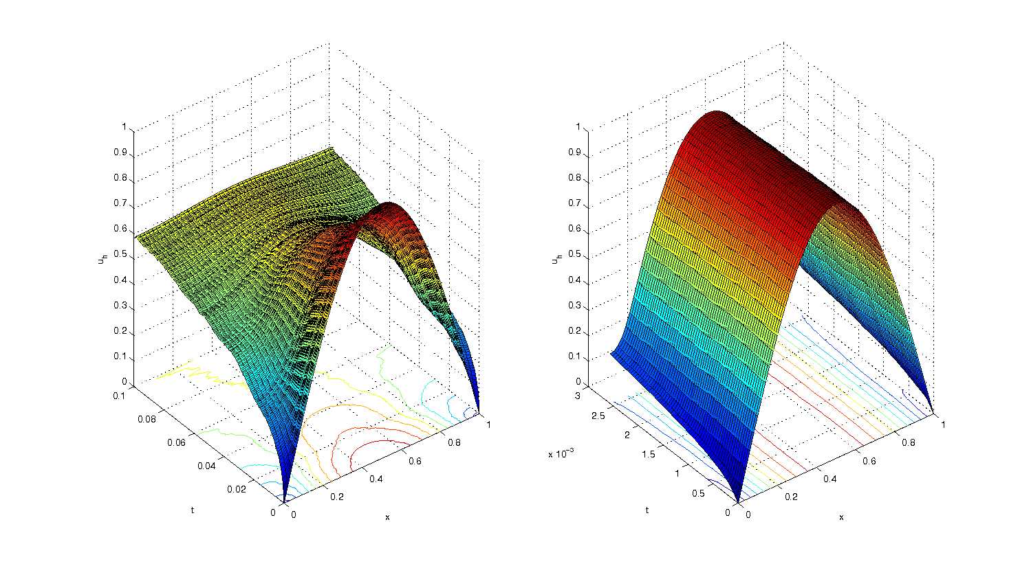
Figure 1. Surface plots of computed solution at a fixed stochastic sample on the space time domains $(0,1)\times(0,0.1)$ (left) and $(0,1)\times(0,2^{8}\times 10^{-5})$ (right). $u_{0}(x)=\sin(\pi x)$ and $\epsilon=0.1$.

Figures 2–4 are the counterparts of Figure 1 with noise intensity parameter $\epsilon=1,\sqrt{2},5$, respectively. We note that the error estimate of Theorem 3.3 does not apply to the latter case because the condition $\epsilon\leq\sqrt{2(1+\delta)}$ is violated. However, the computation result suggests that the stochastic MCF also converges to the steady state solution at the end although the paths to reach the steady state are different for different noise intensity parameter $\epsilon$.

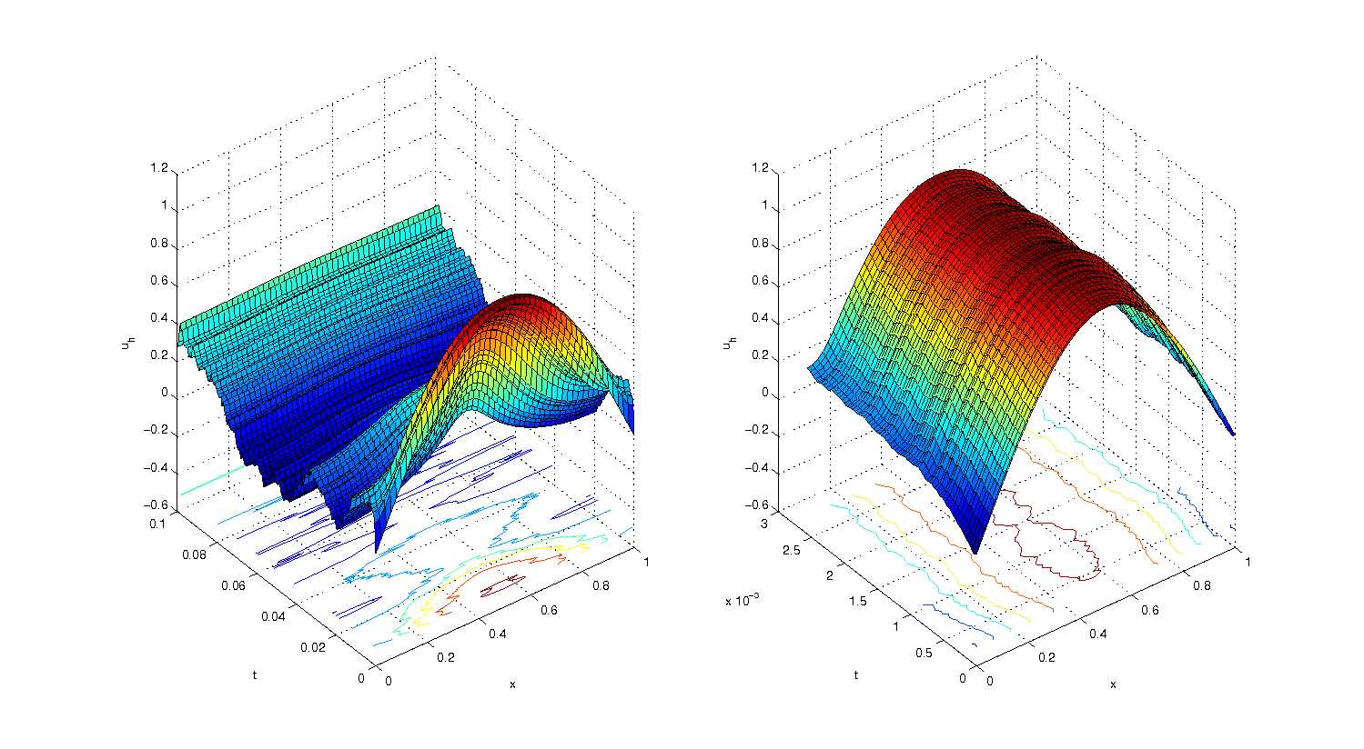
Figure 2. Surface plots of computed solution at a fixed stochastic sample on the space time domains $(0,1)\times(0,0.1)$ (left) and $(0,1)\times(0,2^{8}\times 10^{-5})$ (right). $u_{0}(x)=\sin(\pi x)$ and $\epsilon=1$.

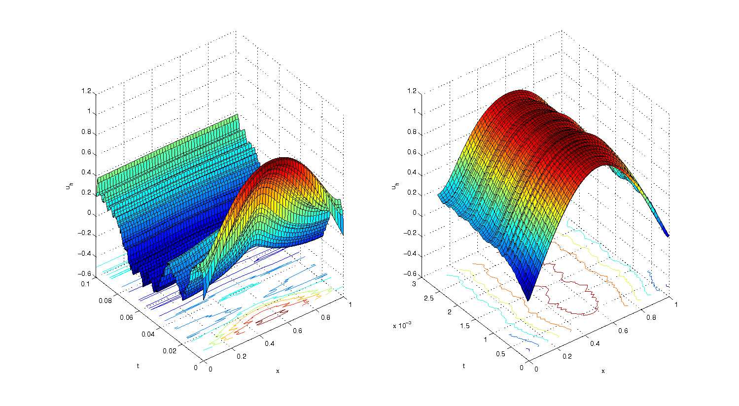
Figure 3. Surface plots of computed solution at a fixed stochastic sample on the space time domains $(0,1)\times(0,0.1)$ (left) and $(0,1)\times(0,2^{8}\times 10^{-5})$ (right). $u_{0}(x)=\sin(\pi x)$ and $\epsilon=\sqrt{2}$.

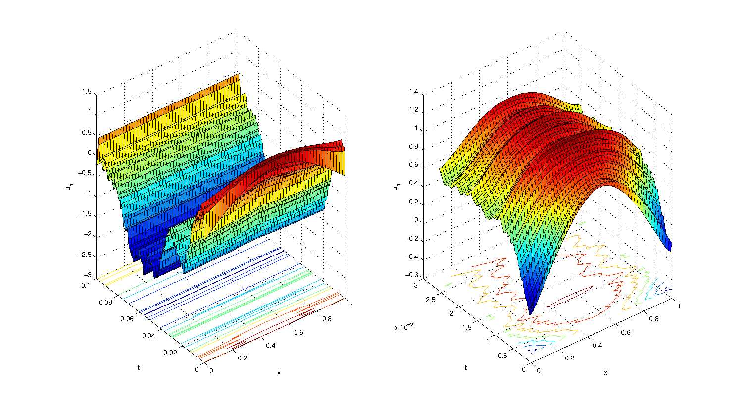
Figure 4. Surface plots of computed solution at a fixed stochastic sample on the space time domains $(0,1)\times(0,0.1)$ (left) and $(0,1)\times(0,2^{8}\times 10^{-5})$ (right). $u_{0}(x)=\sin(\pi x)$ and $\epsilon=5$.

We then repeat the above four tests after replacing the smooth initial function $u_{0}$ by the following non-smooth initial function:

(4.1) $$u_{0}(x)=\begin{cases}10x,&\text{if}\ x\leq 0.25,\\ 5-10x,&\text{if}\ 0.25<x\leq 0.5,\\ 10x-5,&\text{if}\ 0.5<x\leq 0.75,\\ 10-10x,&\text{if}\ 0.75<x\leq 1.\\ \end{cases}$$

The surface plots of the computed solutions are shown in Figures 5–8, respectively. Again, the numerical results suggest that the solution of the stochastic MCF converges to the steady state solution at the end although the paths to reach the steady state are different for different noise intensity parameter $\epsilon$. As expected, the geometric evolution dominates for small $\epsilon$, but the noise dominates the geometric evolution for large $\epsilon$.

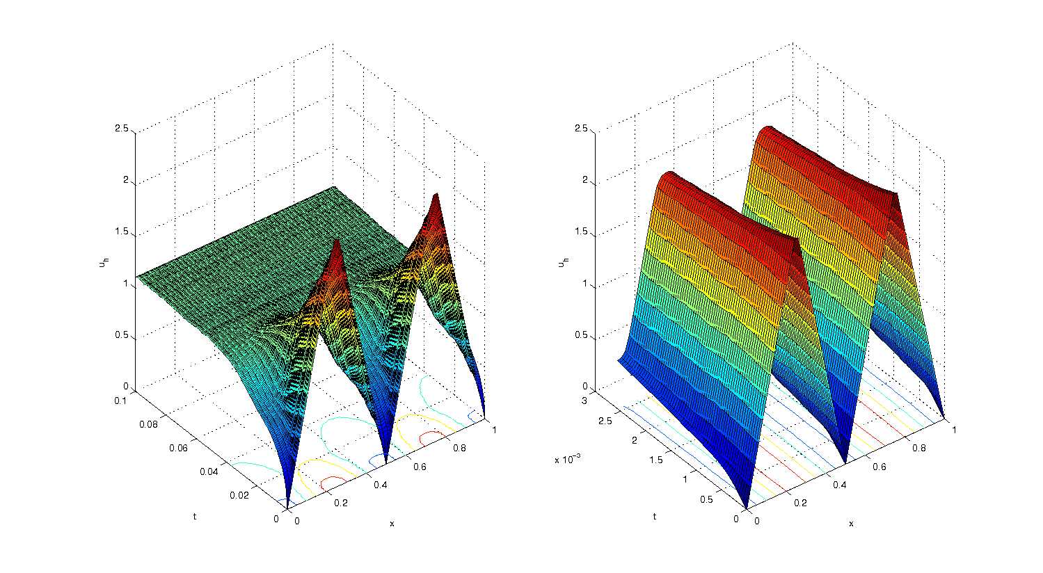
Figure 5. Surface plots of computed solution at a fixed stochastic sample on the space time domains $(0,1)\times(0,0.1)$ (left) and $(0,1)\times(0,2^{8}\times 10^{-5})$ (right). $u_{0}$ is given in (4.1) and $\epsilon=0.1$.

Figure 6. Surface plots of computed solution at a fixed stochastic sample on the space time domains $(0,1)\times(0,0.1)$ (left) and $(0,1)\times(0,2^{8}\times 10^{-5})$ (right). $u_{0}$ is given in (4.1) and $\epsilon=1$.

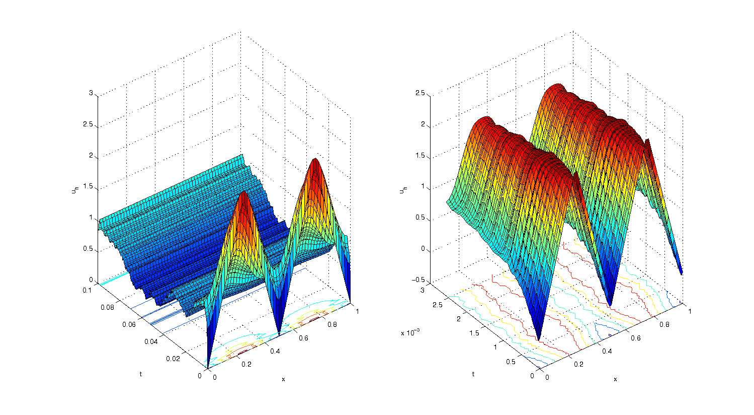
Figure 7. Surface plots of computed solution at a fixed stochastic sample on the space time domains $(0,1)\times(0,0.1)$ (left) and $(0,1)\times(0,2^{8}\times 10^{-5})$ (right). $u_{0}$ is given in (4.1) and $\epsilon=\sqrt{2}$.

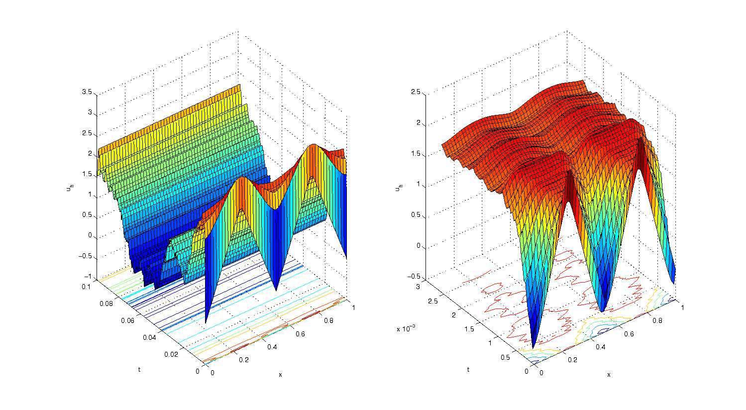
Figure 8. Surface plots of computed solution at a fixed stochastic sample on the space time domains $(0,1)\times(0,0.1)$ (left) and $(0,1)\times(0,2^{8}\times 10^{-5})$ (right). $u_{0}$ is given in (4.1) and $\epsilon=5$.

4.3. Verifying energy dissipation

It follows from (2.5) that the “energy” $J(t):=\frac{1}{2}\mathbb{E}\bigl{[}\|\partial_{x}u^{\delta}(t)\|_{L^{2}(I)}^{2}\bigr{]}$ decreases monotonically in time. In the following we verify this fact numerically. Again, we consider the case with the initial function $u_{0}(x)=\sin(\pi x)$ and the noise intensity parameter $\epsilon=1$. It is not hard to prove that $J(t)$ converges to zero as $t\to\infty$. Figure 9 plots the computed $J(t)$ as a function of $t$. The numerical result suggests that $J(t)$ does not change anymore for $t\geq 0.1$.

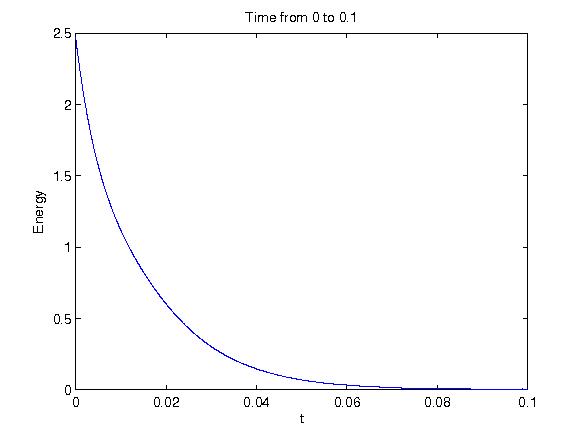
Figure 9. Decay of the energy $J(t)$ on the interval $(0,0.1)$.

4.4. Thresholding for colored noise

In this subsection we present a computational study of the interplay of noise and geometric evolution in (1.5), which is beyond our theoretical results in section 3.1 and 3.2. For this purpose, we use driving colored noise represented by the $Q$-Wiener process ($J\in{\mathbb{N}}$)

(4.2) $$W_{t}=\sum_{j=1}^{J}q_{j}^{\frac{1}{2}}\beta_{j}(t)e_{j}\,,$$

where $\{\beta_{j}(t);\,t\geq 0\}_{j\geq 1}$ denotes a family of real-valued independent Wiener processes on $\bigl{(}\Omega,{\mathcal{F}},{\mathbb{F}},{\mathbb{P}}\bigr{)}$, and $\{(q_{j},e_{j})\}_{j=1}^{J}$ is an eigen-system of the symmetric, non-negative trace-class operator $Q:L^{2}(I)\rightarrow L^{2}(I)$, with $e_{j}=\sqrt{2}\sin(j\pi x)$. In particular, we like to numerically address the following questions:

1. Thresholding: By Theorem 2.1, strong solutions of (1.5) exist for $\varepsilon\leq\sqrt{2}$, and a similar result can be shown for the PDE problem with the noise (4.2). What are admissible intensities of the noise suggested by computations? Moreover, what do the computations suggest about the stochastic MCF in the case of spatially white noise (i.e., $q_{j}\equiv 1,J=\infty$) where no theoretical result is available so far?

2. General initial profiles: The deterministic evolution of Lipschitz initial graphs is well-understood. For example, the (upper) graph of two touching spheres may trigger non-uniqueness. What are the regularization and the noise excitation effects in the case of the initial data with infinite energy and using different noises?

Recall that the estimate in Proposition 3.3 for $V_{r}^{h}$-valued solution $u^{\delta,n}_{h}$ suggests that $\varepsilon>0$ ought be sufficiently small to ensure the existence. In our test, we employ the colored noise (4.2) with $q_{j}^{\frac{1}{2}}=j^{-0.6}$, $J=20$, and the following non-Lipschitz initial data:

(4.3) $$u_{0}(x)=|0.5-x|^{\kappa}\qquad\forall\,x\in(0,1)\,,$$

where $\kappa=0.1$. In addition, we set $(\tau,h)=(0.01,0.02)$ and $T=\frac{1}{2}$. Figure 10 shows the single trajectory of the stochastic MCF plotted as graphs over the space-time domain with, respectively, $\epsilon=0.1,0.5,\sqrt{2}$. The results indicate thresholding, namely, the trajectories grow rapidly in time for sufficiently large values $\varepsilon$, and the noise effect dominates the geometric evolution.

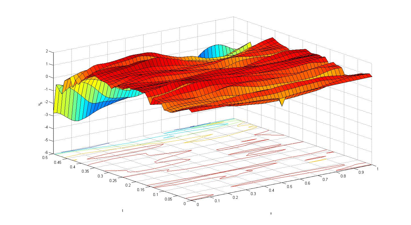
Figure 10. Thresholding for colored noise: Trajectories for $\varepsilon=0.1$ (top left), $\varepsilon=0.5$ (top right), $\varepsilon=\sqrt{2}$ (bottom).

The excitation effect of the noise on the geometric evolution is illustrated by corresponding plots for the evolution of the functional $n\mapsto\|\partial_{x}u_{h}^{\delta,n}(\omega)\|^{2}_{L^{2}}$ vs its expectation $n\mapsto{\mathbb{E}}\bigl{[}\|\partial_{x}u_{h}^{\delta,n}\|^{2}_{L^{2}}\bigr{]}$ in Figure 11 and 12. We observe that the geometric evolution dominates for small values of $\varepsilon$, while the noise evolution takes over for large values of $\varepsilon$.

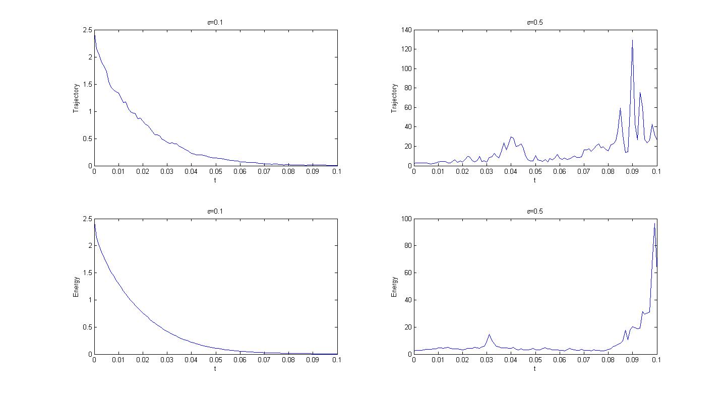
Figure 11. Geometric evolution vs colored noise evolution ($q^{\frac{1}{2}}_{j}=j^{-0.6}$, $J=20$): 1st row: single trajectory for $n\mapsto\|\partial_{x}u_{h}^{\delta,n}(\omega)\|^{2}_{L^{2}}$ and $\varepsilon=0.1$ (left), $\varepsilon=0.5$ (right); 2nd row: $n\mapsto{\mathbb{E}}\bigl{[}\|\partial_{x}u_{h}^{\delta,n}\|^{2}_{L^{2}}\bigr{]}$ for $\varepsilon=0.1$ (left), $\varepsilon=0.5$ (right).

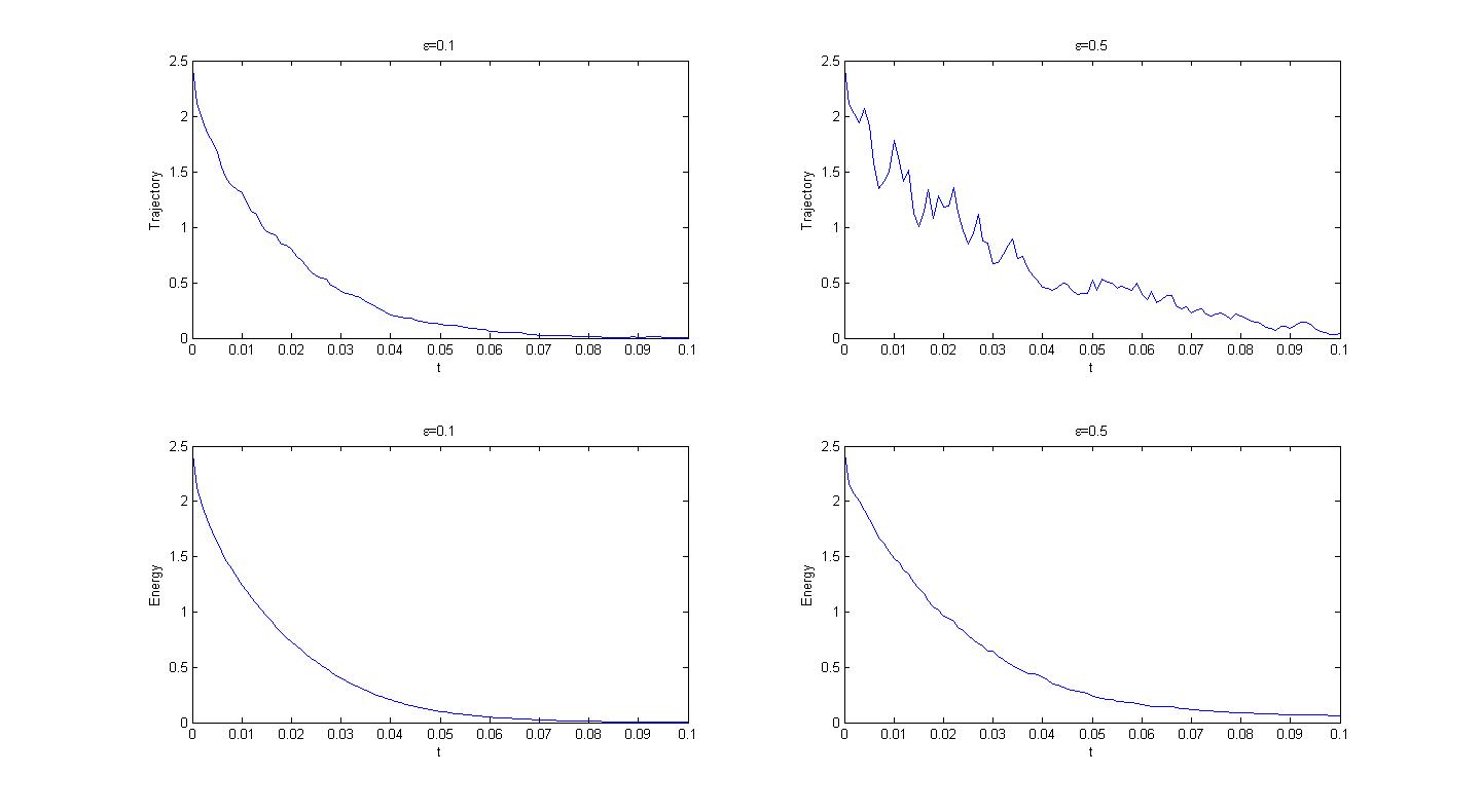
Figure 12. Geometric evolution vs colored noise evolution ($q^{\frac{1}{2}}_{j}=j^{-1}$, $J=50$): 1st row: single trajectory for $n\mapsto\|\partial_{x}u_{h}^{\delta,n}(\omega)\|^{2}_{L^{2}}$ and $\varepsilon=0.1$ (left), $\varepsilon=0.5$ (right); 2nd row: $n\mapsto{\mathbb{E}}\bigl{[}\|\partial_{x}u_{h}^{\delta,n}\|^{2}_{L^{2}}\bigr{]}$ for $\varepsilon=0.1$ (left), $\varepsilon=0.5$ (right).

4.5. Thresholding for white noise

We now consider the case of white noise in (3.20)–(3.21), that is, $q_{j}\equiv 1$ in (4.2) and $J=\infty$, for which the solvability of (1.3) is not known. Figure 13 shows the single trajectory of the stochastic MCF (with the same data as in section 4.4) plotted as graphs over the space-time domain with, respectively, $\epsilon=0.1,0.5,\sqrt{2}$. We observe a very rapid growth of trajectories (numerical values range between $10^{14}$ and $10^{21}$) even for small values of $\varepsilon>0$. These numerical results suggest either a rapid growth or a finite time explosion for the stochastic MCF in the case of white noise.

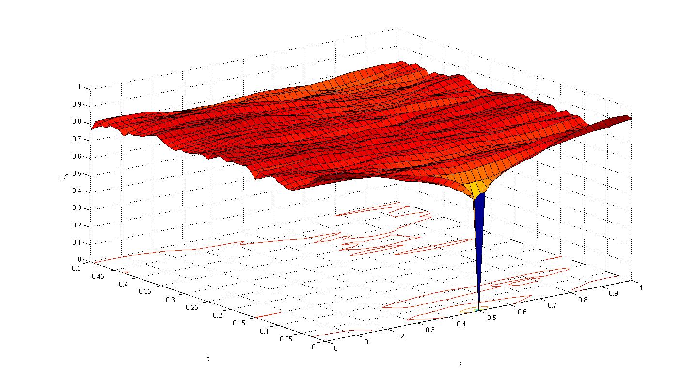
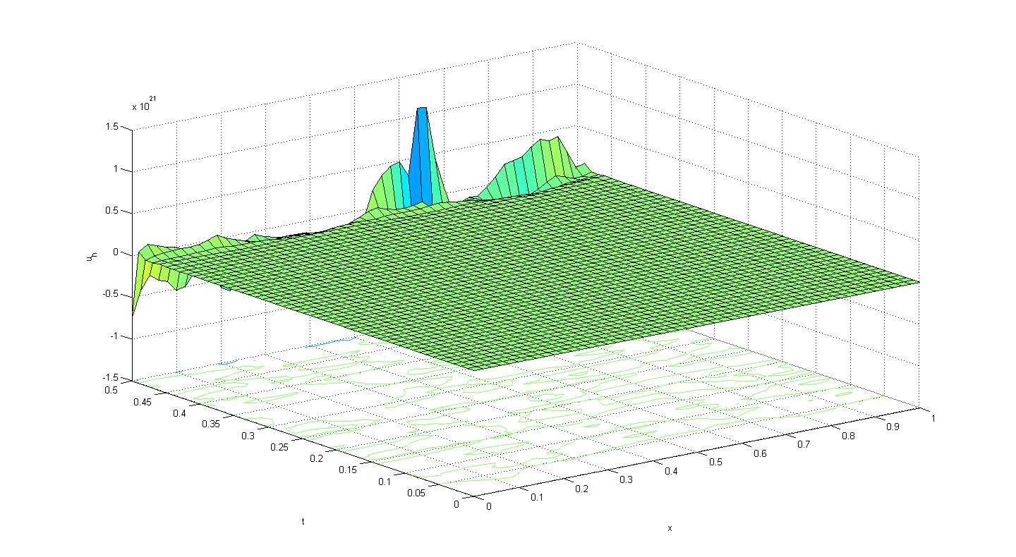
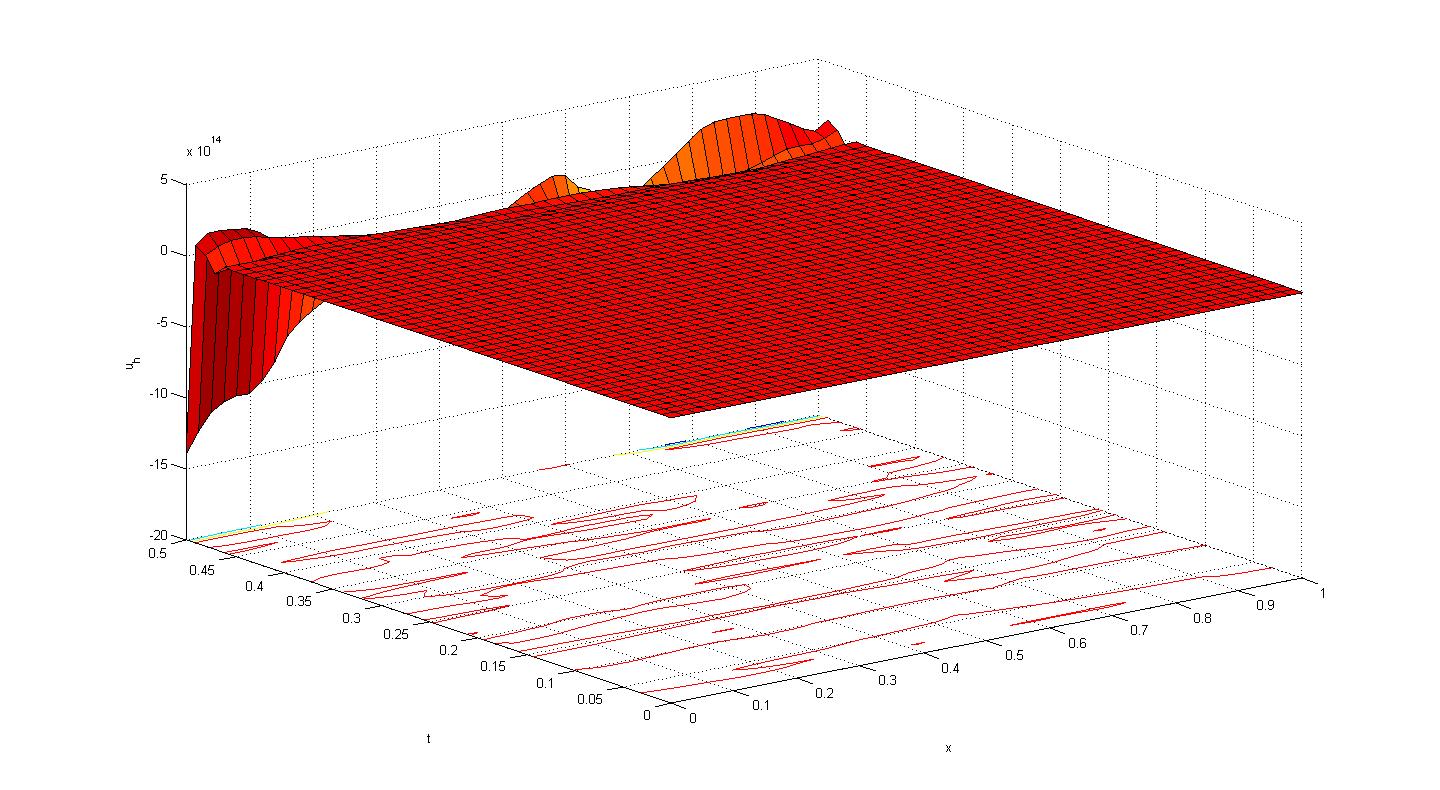
Figure 13. Thresholding and white noise: $\varepsilon=0.1$ (top left), $\varepsilon=0.5$ (top right) $\varepsilon=\sqrt{2}$ (bottom).

References

- [1] F. Almgren, J. E. Taylor, and L. Wang, Curvature-driven flows: a variational approach, SIAM J. Control Optim. 31 (1993), no. 2, 387–438.
- [2] K. A Brakke, The Motion of a Surface by its Mean Curvature, Mathematical Notes 20. Princeton University Press, Princeton, N.J., 1978.
- [3] G. Bellettini and M. Novaga, Minimal barriers for geometric evolutions, J. Differential Equations 139 (1997), no. 1, 76–103.
- [4] G. Bellettini and M. Paolini, Some results on minimal barriers in the sense of De Giorgi applied to driven motion by mean curvature, Rend. Accad. Naz. Sci. XL, Mem. Mat. Appl. (5) 19 (1995), 43–67.
- [5] S. C. Brenner and L. R. Scott, The Mathematical Theory of Finite Element Methods, Second edition, Texts in Applied Mathematics 15. Springer-Verlag, New York, 2002.
- [6] Z. Brzezniak, E. Carelli, A. Prohl, Finite element based discretisations of the incompressible Navier-Stokes equations with multiplicative random forcing, IMA J. Num. Anal. (2013).
- [7] E. Carelli, A. Prohl, Rates of convergence for discretizations of the stochastic incompressible Navier-Stokes equations, SIAM J. Num. Anal., 50 (2012), 2467–2496.
- [8] Y. G. Chen, Y. Giga, and S. Goto, Uniqueness and existence of viscosity solutions of generalized mean curvature flow equations, Proc. Japan Acad. Ser. A, Math. Sci. 65(1989), pp. 207–210.
- [9] E. De Giorgi, Barriers, boundaries, motion of manifolds, Conference held at Department of Mathematics of Pavia, March 18, 1994.
- [10] K. Deckelnick, G. Dziuk, and C. M. Elliott, Computation of geometric partial differential equations and mean curvature flow, Acta Numer. 14 (2005), pp. 139–232.
- [11] K. Ecker and G. Huisken, Mean curvature evolution of entire graphs, Ann. of Math. (2) 130 (1989), no. 3, 453–471.
- [12] A. Es-Sarhir and M. von Renesse, Ergodicity of stochastic curve shortening flow in the plane, SIAM J. Math. Anal., 44 (2013), 224–244.
- [13] L. C . Evans, H. M. Soner and P. E. Souganidis, Phase transitions and generalized motion by mean curvature, Comm. Pure Appl. Math. 45 (1992), no. 9, 1097–112.
- [14] L. C. Evans and J. Spruck, Motion of level sets by mean curvature. I, J. Differential Geom. f 33 (1991), pp. 635–681.
- [15] X. Feng and A. Prohl, Numerical analysis of the Allen-Cahn equation and approximation of the mean curvature flows, Numer. Math. 94 (2003), pp. 33–65.
- [16] Y. Giga, Surface Evolution Equations, A Level Let Approach, Monographs in Mathematics 99. Birkh user Verlag, Basel, 2006.
- [17] I. Gyöngy, A. Millet, Rate of convergence of space time approximations for stochastic evolution equations, Potential Anal. 30 (2009), pp. 29–64.
- [18] G. Huisken, Flow by mean curvature of convex surfaces into spheres, J. Differential Geom. 20 (1984), no. 1, 237–266.
- [19] T. Ilmanen, Convergence of the Allen-Cahn equation to Brakke’s motion by mean curvature, J. Differential Geom. 38 (1993), no. 2, 417–461.
- [20] M. Kovacs, S. Larsson, A. Mesforush, Finite element approximation of the Cahn-Hilliard-Cook equation, SIAM J. Num. Anal. 49, pp. 2407 2429 (2011).
- [21] N. V. Krylov and B. L. Rozovskiǐ, Stochastic evolution equations (Russian), Current problems in mathematics, Vol. 14 (Russian), pp. 71–147, 256, Akad. Nauk SSSR, Vsesoyuz. Inst. Nauchn. Tekhn. Informatsii, Moscow, 1979.
- [22] P. L. Lions and P. E. Souganidis, Fully nonlinear stochastic partial differential equations: non-smooth equations and applications, C. R. Acad. Sci. Paris Sr. I Math. 327 (1998), no. 8, 735–741.
- [23] P. L. Lions and P. E. Souganidis, Fully nonlinear stochastic partial differential equations, C. R. Acad. Sci. Paris Sr. I, Math. 326 (1998), no. 9, 1085–1092.
- [24] S. Osher and R. Fedkiw, Level Set Methods and Dynamic Implicit Surfaces, Applied Mathematical Sciences 153. Springer-Verlag, New York, 2003.
- [25] B. Øksendal, Stochastic differential equations. An introduction with applications, Sixth edition, Universitext, Springer-Verlag, Berlin, 2003.
- [26] S. Osher and J. A. Sethian, Fronts propagating with curvature-dependent speed: algorithms based on Hamilton-Jacobi formulations, J. Comput. Phys. 79 (1988), no. 1, 12–49.
- [27] E. Pardoux, Équations aux dérivées partielles stochastiques de type monotone (French), Séminaire sur les Équations aux Dérivées Partielles (1974 1975), III, Exp. No. 2, page 10. Collége de France, Paris, 1975.
- [28] E. Pardoux, Sur des équations aux dérivées partielles stochastiques monotones (French), C. R. Acad. Sci. Paris Sr. A-B 275 (1972), A101–A103.
- [29] J. A. Sethian, Level Set Methods and Fast Marching Methods. Evolving Interfaces in Computational Geometry, Fluid Mechanics, Computer Vision, and Materials Science, Second edition, Cambridge Monographs on Applied and Computational Mathematics, 3, Cambridge University Press, Cambridge, 1999.
- [30] P. E. Souganidis and N. K. Yip, Uniqueness of motion by mean curvature perturbed by stochastic noise, Ann. Inst. H. Poincar Anal. Non Linaire 21 (2004), no. 1, 1–23.
- [31] N. K. Yip, Stochastic motion by mean curvature, Arch. Rational Mech. Anal. 144 (1998), no. 4, 313–355.
- [32] X. -P. Zhu, Lectures on Mean Curvature Flows, AMS/IP Studies in Advanced Mathematics 32. American Mathematical Society, Providence, RI; International Press, Somerville, MA, 2002.