Compass and Kitaev models – Theory and Physical Motivations

Abstract

Compass models are theories of matter in which the couplings between the internal spin (or other relevant field) components are inherently spatially (typically, direction) dependent. A simple illustrative example is furnished by the “90^∘ compass” model on a square lattice in which only couplings of the form $\tau^{x}_{i}\tau^{x}_{j}$ (where $\{\tau^{a}_{i}\}_{a}$ denote Pauli operators at site $i$) are associated with nearest neighbor sites $i$ and $j$ separated along the $x$ axis of the lattice while $\tau^{y}_{i}\tau^{y}_{j}$ couplings appear for sites separated by a lattice constant along the $y$ axis. Such compass-type interactions appear in diverse physical systems including Mott insulators with orbital degrees of freedom (where interactions sensitively depend on the spatial orientation of the orbitals involved), the low energy effective theories of frustrated quantum magnets, systems with strong spin-orbit couplings (such as the iridates), vacancy centers, and cold atomic gases. Kitaev’s models, in particular the compass variant on the honeycomb lattice, realize basic notions of topological quantum computing. The fundamental inter-dependence between internal (spin, orbital, or other) and external (i.e., spatial) degrees of freedom which underlies compass models generally leads to very rich behaviors including the frustration of (semi-)classical ordered states on non-frustrated lattices and to enhanced quantum effects prompting, in certain cases, the appearance of zero temperature quantum spin liquids. As a consequence of these frustrations, new types of symmetries and their associated degeneracies may appear. These intermediate symmetries lie midway between the extremes of global symmetries and local gauge symmetries and lead to effective dimensional reductions. We review compass models in a unified manner, paying close attention to exact consequences of these symmetries, and to thermal and quantum fluctuations that stabilize orders via order out of disorder effects. We review non-trivial statistics and the appearance of topological quantum orders in compass systems in which, by virtue of their intermediate symmetry standard orders do not arise. This is complemented by a survey of numerical results. Where appropriate theoretical and experimental results are compared.

I Introduction & Outline

I.1 Introduction

This article reviews compass models. The term ”compass models” refers to a family of closely related lattice models involving interacting quantum degrees of freedom (and their classical approximants). Members of this family appear in very different physical contexts. Already three decades ago they were first encountered as minimal models to describe interactions between orbital degrees of freedom in strongly correlated electron materials Kugel & Khomskii (1982). The name orbital compass model was coined at the time, but only in the past decade these models started to receive wide-spread attention to describe physical properties of materials with orbital degrees of freedom Tokura & Nagaosa (2000); van den Brink (2004); Khaliullin (2005a).

In different guises, these models describe the phase variable in certain superconducting Josephson-junction arrays Xu & Moore (2004); Nussinov & Fradkin (2005) and exchange interactions in ultra-cold atomic gasses Duan et al. (2003); Wu (2008). Last but not least, quantum compass models have recently made an entrance to the scene of quantum information theory as mathematical models for topological quantum computing Kitaev (2003): The much-studied Kitaev’s honeycomb model has the structure of a compass model. It is interesting to note that the apparently different fields dealing with orbital degrees of freedom in complex oxides and dealing with models for quantum computing have compass models in common and can thereby in principle cross-fertilize. Kitaev’s honeycomb model has, for instance, been put forward to describe the interactions between magnetic moments in certain iridium-oxide materials Jackeli & Khaliullin (2009).

Here we review the different incarnations of compass models, their physical motivations, symmetries, ordering and excitations. In doing so, we aim to highlight in particular the relation between orbital models and Kitaev’s models for quantum computation. One should stress however that although the investigation of compass and Kitaev models has grown into a considerable area of research, this is an active field of research with still many interesting and open problems, as will become more explicit in the following.

I.2 Outline of the Review

We start by introducing and defining, in Section II, various compass models. Next, in Section III, we discuss viable extensions of more typical compass models including, e.g., ring-exchange and extensions to general spatial dimensions. While the most common representation of compass models is that on a lattice, other representations are noteworthy.

In Section IV, we put to the fore continuum representations that are suited for field theoretic treatments, introduce general momentum space representations and illustrate how it naturally suggests the presence of dimensional reductions in compass models. We furthermore discuss classical incommensurate ground states and the representation of a quantum compass model as an unusual anisotropic classical Ising model. In subsection IV.4, the general equations of motion associated with compass theories are presented; these equations capture the quintessential anisotropic character of the compass models.

Next, in Section V, we discuss the physical contexts that motivate compass models and derive them for special cases. This includes situations where the compass degrees of freedom represent orbital degrees of freedom [subsection V.1]. We review how they emerge, how they interact, and how they are described mathematically in terms of orbital Hamiltonians. Most typical representations rely on SU(2) algebra but we also discuss SU(3) Gell-mann and other matrix forms that are better suited for the description of certain orbital systems. We conclude subsection V.1 by illustrating how strong spin-orbit effects can lead, within the subspace of low-energy locked orbit and spin states, to compass model hybrids, in particular to the so-called Heisenberg-Kitaev model of pertinence to the iridates. A brief summary of how compass models arise vacancy center and trapped ion systems with effective dipolar interactions is provided in subsection V.2. In subsection V.3 we proceed with a review of the realization of compass models in cold atomic systems. We conclude our general discussion of incarnations of compass models in general physical systems in subsection V.4 where we review how the effective low energies theories in chiral frustrated magnets (such as the Kagome and triangular antiferromagnets) are of the compass model type.

In Section VI, we turn to one of the most common unifying features of compass models: the intermediate symmetries that they exhibit. We review what these symmetries are and place in them in perspective to the two extremes of global and local gauge symmetries. We discuss precise consequences of these symmetries notably those concerning effective dimensional reductions, briefly allude to relations to topological quantum orders and illustrate how these symmetries arise in the various compass models.

In Section VII, we introduce a new result: an exact relation between intermediate symmetries and band structures. In particular, we illustrate how flat bands can arise and are protected by the existence of these symmetries and demonstrate how this is materialized in various compass models. One common and important consequence of intermediate symmetries is the presence of an exponentially large ground state degeneracy. We will discuss situations where this degeneracy is exact and ones in which it emerges in various limits.

In Section VIII, we review how low temperature orders in various compass models nevertheless appear and are stabilized by fluctuations or, as they are often termed, order out of disorder effects. Orders in classical compass models that we review are, rigorously, stabilized by thermal fluctuations. This ordering tendency is further bolstered by quantum zero point fluctuations. Due an exact equivalence between the large $n$ and high temperature limits, the low temperature behavior of compass models is supplanted by exact results at high temperatures as review in Section VIII.6.

Following the review of these earlier analytic results concerning the limiting behaviors at both low and high temperatures, we turn in Section IX to numerical results concerning the phases and transitions in various compass model systems. In Section IX.12, we present a discussion (containing both rigorous and numerical results) of the hybrid Heisenberg-Kitaev model and its possible connection to iridate compounds (along with a comparison between theoretical and experimental results).

In the final part of this article, Section X, we review Kitaev’s honeycomb model and its context. This exactly solvable model was inspired by the ideas of topological quantum computing yet also exhibits many other notable features including spin liquid type ground states. Both these aspects we will present and review in a largely self-contained manner.

II Compass Model Overview

II.1 Definition of Quantum Compass Models

In order to define quantum compass models, we start by considering a lattice with sites on which quantum degrees of freedom live. Throughout this review the total number of lattice sites is denoted by by $N$. When square (or cubic) lattices will be involved, these will be consider of dimension $N=L\times L$ (or $N=L\times L\times L$). On more general lattices, $L$ denotes the typical linear dimension (i.e., linear extent along one of the crystalline axis). We set the lattice constant to unity. The spatial dimensionality of the lattice is denoted by $D$ (e.g., $D=2$ for the square and honeycomb lattices, $D=3$ in cubic and pyrochlore lattices etc.).

Depending on the problem at hand, we will refer to these degrees of freedom at the lattice sites as spins, pseudospins or orbitals. We denote these degrees of freedom by $\bm{\tau}_{i}$, where $i$ labels the lattice sites and $\bm{\tau}\equiv\frac{1}{2}(\sigma^{x},\sigma^{y},\sigma^{z})$, where $\sigma^{x}$, $\sigma^{y}$ and $\sigma^{z}$ are the Pauli matrices. In terms of the creation ($c_{\alpha}$) and annihilation ($c^{\dagger}_{\alpha}$) operator for an electron in state $\alpha$, the pseudospin operator ${\bm{\tau}}$ can be expressed as ${\bm{\tau}}=\frac{1}{2}\sum_{\alpha\beta}c^{\dagger}_{\alpha}{\bm{\sigma}}_{\alpha\beta}c_{\beta}$, where the sum if over the two different possibilities for each $\alpha$ and $\beta$. Here $\bm{\tau}$ is the fundamental $T=1/2$ representation of SU(2), for $T>1/2$ we use $\bm{T}$.

A representation in terms of Pauli matrices is particularly useful for degrees of freedom that have two flavors, for instance two possible orientations of a spin (up or down) or two possible orbitals that an electron can occupy, as the Pauli matrices are generators of SU(2), the group of $2\times 2$ matrices with determinant one. For degrees of freedom with $n$ flavors, it makes sense to use a representation in terms of the generators of SU($n$), which for the particular case of $n=3$ are the eight Gell-Mann matrices $\lambda_{i}$, with $i=1,8$ (see Appendix, Sec. XIV).

The name that one chooses to bestow upon the degree of freedom (whether spin, pseudospin, color, flavor or orbital) is of course mathematically irrelevant. For SU(2) quantum compass models it is important that the components of $\bm{\tau}$ obey the well-known commutation relation $[\tau^{x},\tau^{y}]=i\tau^{z}$, and its cyclic permutations and that $(\tau^{\gamma})^{2}=1/4$ for any component $\gamma=x,y,$ or $z$. In the case of SU(3), in the fundamental representation ${\bm{\tau}}$ is the eight component vector ${\bm{\tau}}=\frac{1}{2}\sum_{\alpha\beta}c^{\dagger}_{\alpha}{\bm{\lambda}}_{\alpha\beta}c_{\beta}$, with the commutation relations governed by those of the Gell-Mann matrices.

Compass models are characterized by the specific form that the interaction between the degrees of freedom assumes: $(i)$ there is only an interaction between certain vector components of $\bm{\tau}$ and $(ii)$ on different bonds in the lattice, different vector components interact. When, for instance, a site $i$ is linked to nearest neighbor sites $j$ and $k$, the interaction along the lattice link $\langle ij\rangle$ can be of the type $\tau^{x}_{i}\tau^{x}_{j}$, whereas on the link $\langle ik\rangle$ it is $\tau^{y}_{i}\tau^{y}_{k}$. In the following sections specific Hamiltonians corresponding to various quantum compass models are introduced, in particular the $90^{\circ}$ compass models, Kitaev’s honeycomb model, $120^{\circ}$ compass models and a number of generalizations thereof.

II.1.1 $90^{\circ}$ compass models

A basic realization of a quantum compass model can be set up on a two-dimensional square lattice, where every site has two horizontal and two vertical bonds. If one defines the interaction along horizontal lattice links $\langle ij\rangle_{H}$ to be $J\tau^{x}_{i}\tau^{x}_{j}$ and along the vertical links $\langle ij\rangle_{V}$ to be $J\tau^{y}_{i}\tau^{y}_{j}$, we have constructed the so-called two-dimensional $90^{\circ}$ quantum compass model also known as the planar $90^{\circ}$ orbital compass model, see Fig. 1. Its Hamiltonian is

$$H_{\square}^{90^{\circ}}=-J_{x}\sum_{\langle ij\rangle_{H}}\tau^{x}_{i}\tau^{x}_{j}-J_{y}\sum_{\langle ij\rangle_{V}}\tau^{y}_{i}\tau^{y}_{j}.$$ (1)

The isotropic variant of this system has equal couplings along the vertical and horizontal directions ($J_{x}=J_{y}=J$). The minus signs that appear in this Hamiltonian were chosen such that the interactions between the pseudospins $\bf\tau$ tend to stabilize uniform ground states with ”ferro” pseudospin order. (In $D=2$ the $90^{\circ}$ compass models with ”ferro” and ”antiferro” interactions are directly related by symmetry, see Section II.1.4). For clarity, we note that the isotropic two dimensional compass model is very different from the two-dimensional Ising model

$$H^{Ising}_{\square} = -J\sum_{\langle ij\rangle_{H}}\tau^{x}_{i}\tau^{x}_{j}-J\sum_{\langle ij\rangle_{V}}\tau^{x}_{i}\tau^{x}_{j}$$ (2)

$$= -J\sum_{\langle ij\rangle_{H},\langle ij\rangle_{V}}\tau^{x}_{i}\tau^{x}_{j},$$

where on each horizontal and vertical vertex of the square lattice the interaction is the same and of the form $J\tau^{x}_{i}\tau^{x}_{j}$ – it is also very different from the two-dimensional XY model

$$H^{XY}_{\square}=-J\sum_{\langle ij\rangle_{H},\langle ij\rangle_{V}}(\tau^{x}_{i}\tau^{x}_{j}+\tau^{y}_{i}\tau^{y}_{j}),$$ (3)

because also in this case on all bonds the interaction terms in the Hamiltonian are of the same form.

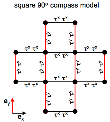
Figure 1: The planar $90^{\circ}$ compass model on a square lattice: the interaction of (pseudo-)spin degrees of freedom ${\bm{\tau}}=(\tau^{x},\tau^{y})$ along horizontal bonds that are connected by the unit vector ${\bf e}_{x}$ is $\tau^{x}_{i}\tau^{x}_{i+{\bf e}_{x}}$. Along vertical bonds ${\bf e}_{y}$ it is $\tau^{y}_{i}\tau^{y}_{i+{\bf e}_{y}}$.

Model Hamiltonian: ${\cal H}=-\sum_{i,\gamma}\tau^{\gamma}_{i}\tau^{\gamma}_{i+\bm{e}_{\gamma}}$
$\{\tau^{\gamma}\}$	$\{\bm{e}_{\gamma}\}$	model name	symbol	dimension
$\{\tau^{x}\}$	$\{\bm{e}_{x}\}$	Ising chain	$H_{1}^{Ising}$	1
$\{\tau^{x},\tau^{y}\}$	$\{\bm{e}_{x},\bm{e}_{x}\}$	XY chain	$H_{1}^{XY}$	1
$\{\tau^{x},\tau^{y},\tau^{z}\}$	$\{\bm{e}_{x},\bm{e}_{x},\bm{e}_{x}\}$	Heisenberg chain	$H_{1}^{Heis}$	1
$\{\tau^{x},\tau^{x}\}$	$\{\bm{e}_{x},\bm{e}_{y}\}$	square Ising	$H_{\square}^{Ising}$	2
$\{\tau^{x},\tau^{x},\tau^{x}\}$	$\{\bm{e}_{x},\bm{e}_{y},\bm{e}_{z}\}$	cubic Ising	$H_{3\square}^{Ising}$	3
$\{\tau^{x},\tau^{y},\tau^{x},\tau^{y}\}$	$\{\bm{e}_{x},\bm{e}_{x},\bm{e}_{y},\bm{e}_{y}\}$	square XY	$H_{\square}^{XY}$	2
$\{\tau^{x},\tau^{y},\tau^{z},\tau^{x},\tau^{y},\tau^{z}\}$	$\{\bm{e}_{x},\bm{e}_{x},\bm{e}_{x},\bm{e}_{y},\bm{e}_{y},\bm{e}_{y}\}$	square Heisenberg	$H_{\square}^{Heis}$	2
$\{\tau^{x},\tau^{y}\}$	$\{\bm{e}_{x},\bm{e}_{y}\}$	90∘ square compass	$H_{\square}^{90^{\circ}}$	2
$\{\tau^{x},\tau^{y},\tau^{z}\}$	$\{\bm{e}_{x},\bm{e}_{y},\bm{e}_{z}\}$	90∘ cubic compass	$H_{3\square}^{90^{\circ}}$	3
With $\{\theta_{\gamma}\}=\{0,2\pi/3,4\pi/3\}$:
$\{\tau^{x},\tau^{x},\tau^{x}\}$	$\bm{e}_{x}\cos{\theta_{\gamma}}+\bm{e}_{y}\sin{\theta_{\gamma}}$	honeycomb Ising	$H_{\varhexagon}^{Ising}$	2
$\{\tau^{x},\tau^{y},\tau^{z}\}$	$\bm{e}_{x}\cos{\theta_{\gamma}}+\bm{e}_{y}\sin{\theta_{\gamma}}$	honeycomb Kitaev	$H_{\varhexagon}^{Kitaev}$	2
$\{\tau^{x},\tau^{x},\tau^{z}\}$	$\bm{e}_{x}\cos{\theta_{\gamma}}+\bm{e}_{y}\sin{\theta_{\gamma}}$	honeycomb XXZ	$H_{\varhexagon}^{XXZ}$	2
$\pi^{\gamma}=\tau^{x}\cos{\theta_{\gamma}}+\tau^{y}\sin{\theta_{\gamma}}$	$\{\bm{e}_{x},\bm{e}_{y},\bm{e}_{z}\}$	cubic 120∘	$H_{3\square}^{120^{\circ}}$	3
$\pi^{\gamma}$	$\bm{e}_{x}\cos{\theta_{\gamma}}+\bm{e}_{y}\sin{\theta_{\gamma}}$	honeycomb 120∘	$H_{\varhexagon}^{120^{\circ}}$	2
With $\{\theta_{\gamma}\}=\{0,2\pi/3,4\pi/3\}$ and $\eta=\pm 1$:
$\{\tau^{x},\tau^{y},\tau^{z}\}$	$\eta\bm{e}_{x}\cos{\frac{\theta_{\gamma}}{2}}+\eta\bm{e}_{y}\sin{\frac{\theta_{\gamma}}{2}}$	triangular Kitaev	$H^{Kitaev}_{\vartriangle}$	2
$\pi^{\gamma}$	$\eta\bm{e}_{x}\cos{\frac{\theta_{\gamma}}{2}}+\eta\bm{e}_{y}\sin{\frac{\theta_{\gamma}}{2}}$	triangular 120∘	$H^{120}_{\vartriangle}$	2

Table 1: Generalized notation that casts compass models and more well-known model Hamiltonians such as the Ising, XY or Heisenberg model on various lattices of different dimensions in the same form. When coupling constants $J_{\gamma}$ depend on the bond direction $\{\bm{e}_{\gamma}$, connecting sites $i$ and $j$, an additional spatial anisotropy is introduced which changes the strengths of the interaction on different links, but not the form of those interactions which is determined by how different components of the vectors ${\bm{\tau}}_{i}$ and ${\bm{\tau}}_{j}$ couple.

One can rewrite the $90^{\circ}$ compass Hamiltonian in a more compact form by introducing unit vectors $\bm{e}_{x}$ and $\bm{e}_{y}$ that denote the bonds along the $x$- and $y$-direction in the 2D lattice, so that

$$H_{\square}^{90^{\circ}}=-J\sum_{i}(\tau^{x}_{i}\tau^{x}_{i+\bm{e}_{x}}+\tau^{y}_{i}\tau^{y}_{i+\bm{e}_{y}}).$$ (4)

With this notation the compass model Hamiltonian can be cast in the more general form

$$H_{\square}^{90^{\circ}}=-J\sum_{i,\gamma}\tau^{\gamma}_{i}\tau^{\gamma}_{i+\bm{e}_{\gamma}},$$ (5)

where for the $90^{\circ}$ square lattice compass model, $H_{\square}^{90^{\circ}}$, we have $\gamma=1,2$, $\{\tau^{\gamma}\}=\{\tau^{1},\tau^{2}\}=\{\tau^{x},\tau^{y}\}$ and $\{\bm{e}_{\gamma}\}=\{\bm{e}_{1},\bm{e}_{2}\}=\{\bm{e}_{x},\bm{e}_{y}\}$.

This generalized notion allows for different compass models and the more well-known models such as the Ising or Heisenberg model to be cast in the same form, see Table 1. For instance the two-dimensional square lattice Ising model $H^{Ising}_{\square}$ corresponds to $\gamma=1,2$ with $\{\tau^{\gamma}\}=\{\tau^{x},\tau^{x}\}$ and $\{\bm{e}_{\gamma}\}=\{\bm{e}_{x},\bm{e}_{y}\}$. The Ising model on a three dimensional cubic lattice is then given by $\gamma=1...3$, $\{\tau^{\gamma}\}=\{\tau^{x},\tau^{x},\tau^{x}\}$ and $\{\bm{e}_{\gamma}\}=\{\bm{e}_{x},\bm{e}_{y},\bm{e}_{z}\}$. The XY model on a square lattice $H^{XY}_{\square}$ corresponds to $\gamma=1...4$, $\{\tau^{\gamma}\}=\{\tau^{x},\tau^{y},\tau^{x},\tau^{y}\}$ and $\{\bm{e}_{\gamma}\}=\{\bm{e}_{x},\bm{e}_{x},\bm{e}_{y},\bm{e}_{y}\}$. Another example is the square lattice Heisenberg model, where we have $\gamma=1...6$, $\{\tau^{\gamma}\}=\{\tau^{x},\tau^{y},\tau^{z},\tau^{x},\tau^{y},\tau^{z}\}$ and $\{\bm{e}_{\gamma}\}=\{\bm{e}_{x},\bm{e}_{x},\bm{e}_{x},\bm{e}_{y},\bm{e}_{y},\bm{e}_{y}\}$, so that in this case $\sum_{\gamma}\tau^{\gamma}_{i}\tau^{\gamma}_{i+\bm{e}_{\gamma}}$ is equal to $\frac{1}{3}\sum_{\gamma}{\bm{\tau}}_{i}\cdot{\bm{\tau}}_{i+\bm{e}_{\gamma}}$.

This class of compass models can be further generalized in a straightforward manner by allowing for a coupling strength $J_{\gamma}$ between the pseudospins $\tau^{\gamma}$ that depends on the direction of the bond $\gamma$ (anisotropic compass models Nussinov & Fradkin (2005)) and by adding a field $h_{\gamma}$ that couples to $\tau^{\gamma}$ linearly Nussinov & Ortiz (2008c); Scarola et al. (2009). This general class of compass models is then defined by the Hamiltonian

$${\cal H}_{compass}=-\sum_{i,\gamma}\left(J_{\gamma}\tau^{\gamma}_{i}\tau^{\gamma}_{i+\bm{e}_{\gamma}}+h_{\gamma}\tau^{\gamma}_{i}\right).$$ (6)

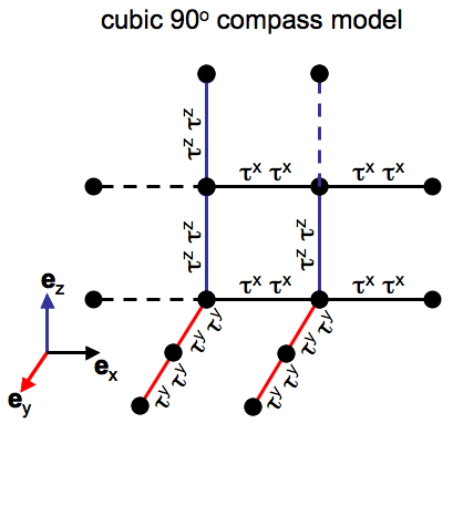
Figure 2: The $90^{\circ}$ compass model on a cubic lattice: the interaction of (pseudo-)spin degrees of freedom ${\bm{\tau}}=(\tau^{x},\tau^{y},\tau^{z})$ along horizontal bonds that are connected by the unit vector ${\bf e}_{x}$ is $J\tau^{x}_{i}\tau^{x}_{i+{\bf e}_{x}}$. On bonds connected by ${\bf e}_{y}$ it is $J\tau^{y}_{i}\tau^{y}_{i+{\bf e}_{y}}$ and along the vertical bonds it is $J\tau^{z}_{i}\tau^{z}_{i+{\bf e}_{z}}$.

From a historical (as well as somewhat practical) viewpoint the three dimensional 90^∘ compass model is particularly interesting. Denoted by $H_{3\square}^{90^{\circ}}$, it is customarily defined on a cubic lattice and given by $\cal H$ (Eq. (6)) where $\gamma$ spans three Cartesian directions: $\gamma=1...3$ with $\{\tau^{\gamma}\}=\{\tau^{x},\tau^{y},\tau^{y}\}$, $J_{\gamma}=J=1$, $h_{\gamma}=0$ and $\{\bm{e}_{\gamma}\}=\{\bm{e}_{x},\bm{e}_{y},\bm{e}_{z}\}$, so that

$$H_{3\square}^{90^{\circ}}=-J\sum_{i}(\tau^{x}_{i}\tau^{x}_{i+\bm{e}_{x}}+\tau^{y}_{i}\tau^{y}_{i+\bm{e}_{y}}+\tau^{z}_{i}\tau^{z}_{i+\bm{e}_{z}}).$$ (7)

Thus, the square lattice 90 degree compass model of Eq. (5) is trivially extended to three spatial dimensions by allowing $\gamma$ to assume values $\gamma=1,2,3$, Thus, with appropriate generalizations, in an arbitrary spatial dimension $D$ (which we will return to in later sections), $\gamma=1,2,...,D$. The structure of this Hamiltonian is schematically represented in Fig. 2. This compass model is actually the one that was originally proposed by Kugel & Khomskii (1982) in the context of orbital ordering. At that time it was noted that even if the interaction on each individual bond is Ising-like, the overall symmetry of the model is considerably more complicated, as will be reviewed in Sec. V.1.

In alternative notations for compass model Hamiltonians one introduces the unit vector $\bm{n}$ connecting neighboring lattice sites $i$ and $j$. Along the three Cartesian axes on a cubic lattice, for instance, ${\bm{n}}$ equals $\bm{e}_{x}=(1,0,0)$, $\bm{e}_{y}=(0,1,0)$ or $\bm{e}_{z}=(0,0,1)$. With this one can express $\tau^{x}$ as $\tau^{x}=\bm{\tau}\cdot\bm{e}_{x}$ and with this vector notation

$$H_{3\square}^{90^{\circ}}=-\sum_{i,\gamma}\tau^{\gamma}_{i}\tau^{\gamma}_{i+\bm{e}_{\gamma}}=-\sum_{ij}\left(\bm{\tau}_{i}\cdot{\bm{n}}\right)\left(\bm{\tau}_{j}\cdot{\bm{n}}\right).$$ (8)

The Hamiltonian in vector form stresses the compass nature of the interactions between the pseudospins. The vector notation, however, not always generalizes naturally to cases with higher dimensions and/or different lattice geometries. All Hamiltonians in this review will therefore be given in terms $\tau^{\gamma}$ operators and be complemented by an expression in vector notation where appropriate.

It is typical for compass models that even the ground state structure is non-trivial. For a system governed by $H_{3\square}^{90^{\circ}}$, pairs of pseudospins on lattice links parallel to the $x$-axis, for instance, favor pointing their pseudospins $\bm{\tau}$ along $x$ so that the expectation value $\langle\tau^{x}\rangle\neq 0$, see Fig. 3. Similarly, on bonds parallel to the $y$-direction, it is advantageous for the pseudospins to align along the $y$ direction, so that $\langle\tau^{y}\rangle\neq 0$. It is clear that at a site the bonds along $x$, $y$ and $z$ cannot be satisfied at the same time, so that the interactions are in fact strongly frustrated. This situation bears resemblance to the dipole-dipole interactions between magnetic needles positioned on a lattice, and hence the Hamiltonian above was coined a compass model.

Such a frustration of interactions is typical of compass models, but of course also appears in numerous other systems. Indeed, on a conceptual level, many of the ideas and results that will be discussed in this review such as renditions of thermal and quantum fluctuation-driven ordering effects, unusual symmetries and ground state sectors labeled by topological invariants have similar incarnations in frustrated spin, charge, cold atom and Josephson junction array systems. Although these similarities are mostly conceptual there are also instances where there are exact correspondences. For instance, the two dimensional 90^∘ compass model is, in fact, dual to the Moore-Lee model describing Josephson coupling between superconducting grains in a square lattice Xu & Moore (2005, 2004); Moore & Lee (2004) that exhibits time reversal symmetry breaking Nussinov & Fradkin (2005); Cobanera et al. (2010).

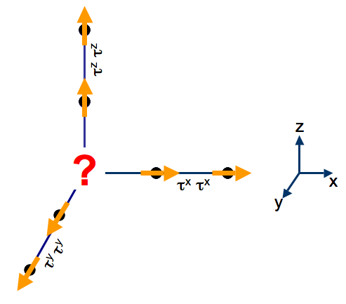
Figure 3: Frustration in the $90^{\circ}$ compass model on a cubic lattice. The interactions between pseudospins $\bm{\tau}$ are such that the pseudospins tend to align their components $\tau^{x}$, $\tau^{y}$ and $\tau^{z}$ along the $x$, $y$ and $z$-axis, respectively. This causes mutually exclusive ordering patterns.

II.1.2 Kitaev’s honeycomb model

In 2006, Alexei Kitaev introduced a type of compass model that has interesting topological properties and excitations, which are relevant and much studied in the context of topological quantum computing Kitaev (2006). The model is defined on a honeycomb lattice and is referred to either as Kitaev’s honeycomb model or the XYZ honeycomb compass model. The lattice links on a honeycomb lattice may point along three different directions, see Fig. 4. One can label the bonds along these directions by $\bm{e}_{1}$, $\bm{e}_{2}$ and $\bm{e}_{3}$, where the angle between the three unit lattice vectors is $120^{\circ}$. With these preliminaries, the Kitaev’s honeycomb model Hamiltonian $H_{\varhexagon}^{Kitaev}$ reads

$$-J_{x}\sum_{\begin{smallmatrix}\bm{e}_{1}-&\\ {\sf bonds}&\end{smallmatrix}}\tau^{x}_{i}\tau^{x}_{j}-J_{y}\sum_{\begin{smallmatrix}\bm{e}_{2}-&\\ {\sf bonds}&\end{smallmatrix}}\tau^{y}_{i}\tau^{y}_{j}-J_{z}\sum_{\begin{smallmatrix}\bm{e}_{3}-&\\ {\sf bonds}&\end{smallmatrix}}\tau^{z}_{i}\tau^{z}_{j}.$$

One can re-express this model in the form of $H_{compass}$ introduced above, where

$$H_{\varhexagon}^{Kitaev} = -\sum_{i,\gamma}J_{\gamma}\tau^{\gamma}_{i}\tau^{\gamma}_{i+\bm{e}_{\gamma}}$$ (13)

$$with\left\{\begin{array}[]{l}\{\tau^{\gamma}\}=\{\tau^{x},\tau^{y},\tau^{z}\}\\ \{J_{\gamma}\}=\{J_{x},J_{y},J_{z}\}\\ \bm{e}_{\gamma}=\bm{e}_{x}\cos{\theta_{\gamma}}+\bm{e}_{y}\sin{\theta_{\gamma}}\\ \{\theta_{\gamma}\}=\{0,2\pi/3,4\pi/3\}\end{array}\right.$$

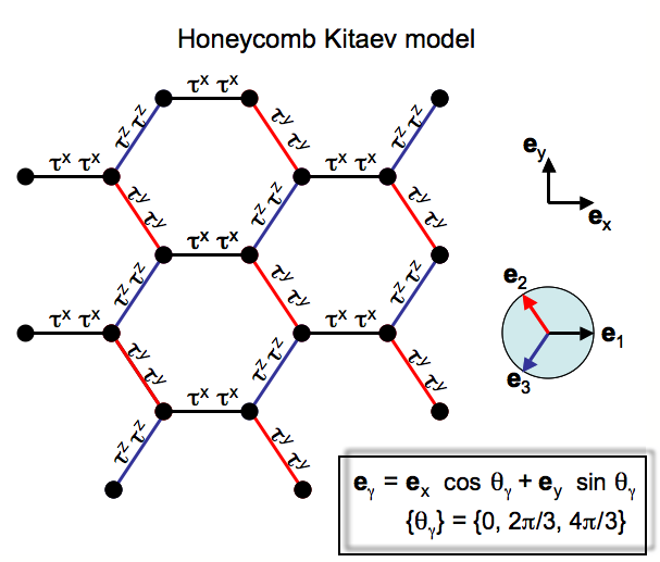
Figure 4: Kitaev’s compass model on a honeycomb lattice: the interaction of (pseudo-)spin degrees of freedom ${\bm{\tau}}=(\tau^{x},\tau^{y},\tau^{z})$ along the three bonds that each site is connected to are $\tau^{x}_{i}\tau^{x}_{i+{\bf e}_{1}}$, $\tau^{y}_{i}\tau^{y}_{i+{\bf e}_{2}}$ and $\tau^{z}_{i}\tau^{z}_{i+{\bf e}_{z}}$, where the bond-vectors of the honeycomb lattice $\{{\bf e}_{1},{\bf e}_{2},{\bf e}_{3}\}$ are $\{{\bf e}_{x},-{\bf e}_{x}/2+\sqrt{3}{\bf e}_{y}/2,-{\bf e}_{x}/2-\sqrt{3}{\bf e}_{y}/2\}$, respectively.

It was proven that for large $J_{z}$, the model Hamiltonian $H_{\varhexagon}^{Kitaev}$ maps onto a square lattice model known as Kitaev’s toric code model Kitaev (2003). We will return to these models of Kitaev in Sec. X and discuss there other related quantum computing models. Numerous other aspects of these models have been investigated in great depth. These include, amongst others, issues pertaining to quench dynamics Mondal et al. (2008); Sengupta et al. (2008); Sen & Vishveshwara (2010). Related hybrid models (see sections II.2, V.1.8, IX.12) were suggested to be of relevance to certain iridium oxide materials. To highlight the pertinent interactions and geometry of Kitaev’s honeycomb model as a compass model, it may also be termed an XYZ honeycomb compass model. It suggests variants such as the XXZ honeycomb compass model which we define next.

II.1.3 The XXZ honeycomb compass model

A variation of the Kitaev honeycomb compass Hamiltonian $H_{\varhexagon}^{Kitaev}$ in Eq. (13) is to consider a compass model where on bonds in two directions there is an $\tau^{x}\tau^{x}$-type interaction and in the third direction a $\tau^{z}\tau^{z}$ interaction. This model goes under the name of the XXZ honeycomb compass model Nussinov et al. (2012a). Explicitly, it is given by the Hamiltonian

$$H_{\varhexagon}^{XXZ} = -\sum_{i,\gamma}J_{\gamma}\tau^{\gamma}_{i}\tau^{\gamma}_{i+\bm{e}_{\gamma}}$$ (18)

$$with\left\{\begin{array}[]{l}\{\tau^{\gamma}\}=\{\tau^{x},\tau^{x},\tau^{z}\}\\ \{J_{\gamma}\}=\{J_{x},J_{x},J_{z}\}\\ \bm{e}_{\gamma}=\bm{e}_{x}\cos{\theta_{\gamma}}+\bm{e}_{y}\sin{\theta_{\gamma}}\\ \{\theta_{\gamma}\}=\{0,2\pi/3,4\pi/3\}\end{array}\right.$$

A schematic is provided in Fig. 5. The key defining feature of this Hamiltonian vis a vis the original Kitaev model of Section II.1.2- the interactions along both the diagonal (“zig-zag”) - “x” and “y”- directions of the honeycomb lattice are of the $\tau^{x}\tau^{x}$ type (as opposed to both $\tau^{x}\tau^{x}$ and $\tau^{y}\tau^{y}$ in Kitaev’s model). Similar to Kitaev’s honeycomb model, all interactions along the vertical (“z” direction) are of the $\tau^{z}\tau^{z}$ type. While in Eq. (18) only two couplings, $J_{x}$ and $J_{z}$, appear, the model can of course be further generalized to having three different couplings on the three different types of links (and more generally to have non-uniform spatially dependent couplings), while the interactions retain their $XXZ$ form. In all of these cases, an exact duality to a corresponding Ising lattice gauge theory on a square lattice which we will elaborate on in later in this review (Section IX.8) exists.

Figure 5: Schematic representation of the XXZ honeycomb compass model Nussinov et al. (2012a).

II.1.4 120^∘ compass models

The 120^∘ compass model has the form of $H_{compass}$ (Eq. (6)) and is defined on a general lattice having three distinct lattice directions ${\bm{e}}_{\gamma}$ for nearest neighbor links. As for the other compass models on these lattice links different components of $\bm{\tau}$ interact. Its particularity is that the three components of $\bm{\tau}$ are not orthogonal. Along bond $\gamma$ the interaction is between the vector components $\tau^{x}\cos{\theta}+\tau^{y}\sin{\theta}$ of the two sites connected by the bond, where for the three different links of each site $\theta=0,2\pi/3$ and $4\pi/3$ respectively.

The model was first studied on the cubic lattice Nussinov et al. (2004); Biskup et al. (2005); van den Brink (2004) and later on the honeycomb Nasu et al. (2008); Wu (2008); Zhao & Liu (2008) and pyrochlore lattice Chern et al. (2010). The general $120^{\circ}$ Hamiltonian can be denoted as

$$H^{120}=-J\sum_{i,\gamma=1...3}\hat{\pi}^{\gamma}_{i}\hat{\pi}^{\gamma}_{i+{\bm{e}}_{\gamma}},$$ (19)

where $\hat{\pi}^{\gamma}_{i}$ are the three projections of $\tau$ along three equally spaced directions on a unit disk in the $xy$-plane:

$$\begin{array}[]{l}\hat{\pi}^{1}=\tau^{x},\\ \hat{\pi}^{2}=-(\tau^{x}-\sqrt{3}\tau^{y})/2\\ \hat{\pi}^{3}=-(\tau^{z}+\sqrt{3}\tau^{x})/2.\end{array}$$ (23)

Hence the name 120^∘ model. In the notation of $H_{compass}$ in Eq. (6) the $120^{\circ}$ Hamiltonian on a 3D cubic lattice, represented in Fig. 6, takes the form

$$H^{120}_{3\square} = -J\sum_{i,\gamma}\hat{\pi}^{\gamma}_{i}\hat{\pi}^{\gamma}_{i+\bm{e}_{\gamma}}$$ (27)

$$with\left\{\begin{array}[]{l}\hat{\pi}^{\gamma}=\tau^{x}\cos{\theta_{\gamma}}+\tau^{y}\sin{\theta_{\gamma}}\\ \{\bm{e}_{\gamma}\}=\{\bm{e}_{x},\bm{e}_{y},\bm{e}_{z}\}\\ \{\theta_{\gamma}\}=\{0,2\pi/3,4\pi/3\}.\end{array}\right.$$

Similar to the $90^{\circ}$ compass model, the bare $120^{\circ}$ model can be extended to include anisotropy of the coupling constants $J_{\gamma}$ along the different crystalline directions and external fields van Rynbach et al. (2010). On a honeycomb lattice the $120^{\circ}$ Hamiltonian Nasu et al. (2008); Wu (2008); Zhao & Liu (2008) can be thought of as a breed of $H^{120}_{3\square}$ and $H^{Kitaev}_{\varhexagon}$:

$$H^{120}_{3\varhexagon} = -J\sum_{i,\gamma}\pi^{\gamma}_{i}\pi^{\gamma}_{i+\bm{e}_{\gamma}}$$ (31)

$$with\left\{\begin{array}[]{l}\pi^{\gamma}=\tau^{x}\cos{\theta_{\gamma}}+\tau^{y}\sin{\theta_{\gamma}}\\ \bm{e}_{\gamma}=\bm{e}_{x}\cos{\theta_{\gamma}}+\bm{e}_{y}\sin{\theta_{\gamma}}\\ \{\theta_{\gamma}\}=\{0,2\pi/3,4\pi/3\}.\end{array}\right.$$

It is worth highlighting the differences and similarity between the models of Eqs. (27, 31) on the cubic and honeycomb lattices respectively. Although the pseudo-spin operators that appear in these two equations have an identical form, they correspond to different physical links. In the cubic lattice, bonds of the type $\hat{\pi}^{\gamma}_{i}\hat{\pi}^{\gamma}_{i+\bm{e}_{\gamma}}$ are associated with links along the Cartesian $\gamma$ directions; on the honeycomb lattice, bonds of the type $\pi^{\gamma}_{i}\pi^{\gamma}_{i+\bm{e}_{\gamma}}$ correspond to links along the three possible orientations of nearest neighbor links in the two dimensional honeycomb lattice.

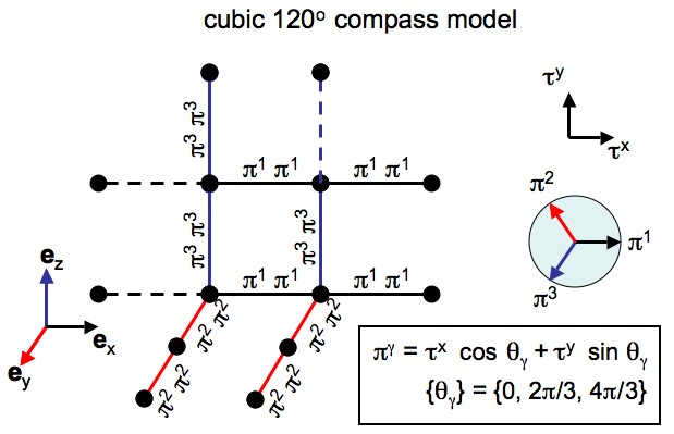
Figure 6: The $120^{\circ}$ compass model on a cubic lattice: the interaction of (pseudo-)spin degrees of freedom ${\bm{\tau}}=(\tau^{x},\tau^{y},\tau^{z})$ along the three bonds that each site is connected to are $\hat{\pi}^{1}_{i}\hat{\pi}^{1}_{i+{\bf e}_{x}}$, $\hat{\pi}^{2}_{i}\hat{\pi}^{2}_{i+{\bf e}_{y}}$ and $\hat{\pi}^{3}_{i}\hat{\pi}^{3}_{i+{\bf e}_{z}}$, where the different components $\{\hat{\pi}^{1},\hat{\pi}^{2},\hat{\pi}^{3}\}$ of the vector $\hat{\bm{\pi}}=(\tau^{x},(-\tau^{x}+\sqrt{3}\tau^{y})/2,(-\tau^{x}-\sqrt{3}\tau^{y})/2)$ interact along the different bonds $\{{\bf e}_{x},{\bf e}_{y},{\bf e}_{z}\}$.

In 120^∘ compass models the interactions involve only two of the components of $\bf{\tau}$ (so that $n=2$) as opposed to three component “Heisenberg” character of the three dimensional $90^{\circ}$ compass system, having $n=3$. In that sense 120^∘ models are similar XY models. On bipartite lattices, the ferromagnetic (with $J>0$) and antiferromagnetic ($J<0$) variants of the 120^∘ compass model are equivalent to one another up to the standard canonical transformation involving every second site of the bipartite lattice. This can be made explicit by defining the operator

$$U=\prod_{i=odd}\tau^{z}_{i},$$ (32)

with the product taken over all sites $i$ that belong to, e.g., the odd sublattice for which the sum of the components of the lattice site along the three Cartesian directions, $i_{x}+i_{y}+i_{z}$, is an odd integer. The unitary mapping $U^{\dagger}H_{120}U$ then effects a change of sign of the interaction constant $J$ (i.e., $J\to-J$). The ferro and antiferro square lattice $90^{\circ}$ compass model $(H^{90^{\circ}}_{\square})$ are related to one another in the same way as, similarly, in this case $n=2$. It should be noted that this mapping does not hold for the 3D rendition of the $90^{\circ}$ model: in this case the interactions also involve $\tau^{z}$ and consequently $H^{90^{\circ}}_{3\square}$ has different low temperature statistical mechanical properties for $J>0$ and $J<0$.

The 120^∘ models have also appeared in various physical contexts on non bipartite lattices. On the triangular lattice Mostovoy & Khomskii (2002); Wu (2008); Zhao & Liu (2008), the model is given by

$$H^{120}_{3\vartriangle} = -J\sum_{i,\gamma,\eta}\pi^{\gamma}_{i}\pi^{\gamma}_{i+\eta\bm{e}_{\gamma}}$$ (37)

$$with\left\{\begin{array}[]{l}\pi^{\gamma}=\tau^{x}\cos{\theta_{\gamma}}+\tau^{y}\sin{\theta_{\gamma}}\\ \bm{e}_{\gamma}=\bm{e}_{x}\cos\frac{\theta_{\gamma}}{2}+\bm{e}_{y}\sin\frac{\theta_{\gamma}}{2}\\ \{\theta_{\gamma}\}=\{0,2\pi/3,4\pi/3\}\\ \eta=\pm 1.\end{array}\right.$$

The triangular model is very similar to the honeycomb lattice model of Eq. (31). The notable difference is that in the triangular lattice there are additional links: In the triangular lattice, each site has six nearest neighbor whereas on the honeycomb lattice, each site has three nearest neighbors. In the Hamiltonian of Eq. (37), nearest neighbor interactions of the $\pi^{1}\pi^{1}$ type appear for nearest neighbor interactions along the rays parallel to the ${\bm{e}}_{x}$ direction (i.e., appear, for a given site to its two neighbors at angles of zero or 180^∘ relative to the ${\bm{e}}_{1}$ crystalline directions). Similarly, interactions of the $\pi^{2,3}\pi^{2,3}$ type appear for rays parallel to the other two crystalline directions.

II.2 Hybrid Compass Models

An interesting and relevant extension of the bare compass models is one in which both usual SU(2) symmetric Heisenberg-type exchange terms $\bm{\tau_{i}}\cdot\bm{\tau_{j}}$ appear in unison with the directional bonds of the bare $90^{\circ}$ or $120^{\circ}$ compass model, resulting in compass-Heisenberg Hamiltonians of the type

$$H=-\sum_{i,\gamma}(J_{H}\bm{\tau_{i}}\cdot\bm{\tau}_{i+\bm{e}_{\gamma}}+J_{K}\tau^{\gamma}_{i}\tau^{\gamma}_{i+\bm{e}_{\gamma}}),$$ (38)

where $J_{H}$ denotes the coupling constant for the interactions of Heisenberg form and $J_{K}$ the coupling constant of the compass or Kitaev terms in the Hamiltonian. For instance the $120^{\circ}$ rendition of this Hamiltonian lattice has been considered on a honeycomb lattice, where it describes exchange interactions between the magnetic moments Ir⁴⁺ ions in a family of layered iridates A₂IrO₃ (A= Li, Na) – materials in which the relativistic spin-orbit coupling plays an important role Chaloupka et al. (2010); Trousselet et al. (2011). The hybrid $90^{\circ}$ Heisenberg-compass model was introduced in the context of interacting $t_{2g}$ orbital degrees of freedom van den Brink (2004) and its 2D quantum incarnation was studied by Trousselet et al., 2010. Another physical context in which such a hybrid model appears is the modeling of the consequences of the presence of orbital degrees of freedom in LaTiO₃ on the magnetic interactions in this material Khaliullin (2001). We will review in detail these resulting Heisenberg-compass and Heisenberg-Kitaev models Chaloupka et al. (2010); Reuther et al. (2011) and its physical motivations in Sec. V.1.8 and Sec. IX.12.

In a very similar manner hybrids of Ising and compass models be constructed. An Ising-compass Hamiltonian of the form $H_{\square}^{90^{\circ}}+H_{\square}^{Ising}$ has for instance been introduced and studied by Brzezicki & Oleś, 2010.

III Generalized & Extended Compass Models

Thus far, we focused solely only a single pseudospin at a given site. It is also possible to consider situations in which more than one pseudospin appears at a site or with a coupling between pseudospins and usual spin degrees of freedom – a situation equivalent to having two pseudospin degrees of freedom per site. Kugel-Khomskii (KK) models comprise a class of Hamiltonians that are characterized by having both spin and pseudospin (orbital) degrees of freedom on each site. These models are introduced in the next Section but their physical incarnations will be reviewed in detail in Sec. V. The KK models are reviewed in Sec. III.1 followed by a possible generalization that we briefly introduce and discuss which includes multiple pseudo-spin degrees of freedom. We will then discuss, in Sec. III.2, extensions of the quantum compass models introduced earlier to the classical arena, to higher dimensions and to large number of spin components $n$. In Sec. III.3 we collect other compass model extensions.

III.1 Kugel-Khomskii Spin-Orbital Models

The situation in which at a site both pseudospin and usual spin degrees of freedom are present naturally occurs in the realm of orbital physics. It arises when (electron) spins can occupy different orbital states of an ion – the orbital degree of freedom or pseudospin. The spin and orbital degree of freedom couple to each other because the inter-site spin-spin interaction depends on the orbital states of the two spins involved. Hamiltonians that result from such a coupling of spin and orbital degrees of freedom are generally know as Kugel-Khomskii (KK) model Hamiltonians, after the authors that have first derived Kugel & Khomskii (1972, 1973) and reviewed them Kugel & Khomskii (1982) in a series of seminal papers. Later reviews include Tokura & Nagaosa (2000); Khaliullin (2005a)

The physical motivation and incarnations of such KK spin-orbital models will be discussed in Sec. V.1. In Sec. V.1.4 they will be derived for certain classes of materials from models of their microscopic electronic structure, in particular from the multi-orbital Hubbard model in which the electron-hopping integrals $t_{i,j}^{\alpha\beta}$ between orbital $\alpha$ on lattice site $i$ and $\beta$ on site $j$ and the Coulomb interactions between electrons in orbitals on the same site are the essential ingredients. A KK Hamiltonian then emerges as the low-energy effective model of a multi-orbital Hubbard system in the Mott insulating regime, when there is on average an integer number of electrons per site and Coulomb interactions are strong. In that case charge excitations are suppressed because of a large gap and the low energy dynamics is governed entirely by the spin and orbital degrees of freedom. In this Section we introduce the generic structure of KK models. Generally speaking the interaction between spin and orbital degrees of freedom on site $i$ and neighboring site $i+\bm{e}_{\gamma}$ is the product of usual spin-spin exchange interactions and compass-type orbital-orbital interactions on this particular bond. The generic structure of the KK models therefore is

$$H^{KK}=-J_{KK}\sum_{i,\gamma}H^{orbital}_{i,i+\bm{e}_{\gamma}}H^{spin}_{i,i+\bm{e}_{\gamma}}.$$ (39)

$H^{orbital}_{i,i+\bm{e}_{\gamma}}$ are operators that act on the pseudospin (orbital) degrees of freedom ${\bm{\tau}}_{i}$ and ${\bm{\tau}}_{i+\bm{e}_{\gamma}}$ on sites $i$ and $i+\bm{e}_{\gamma}$ and $H^{spin}_{i,i+\bm{e}_{\gamma}}$ acts on the spins ${\bm{S}}_{i}$ and ${\bm{S}}_{i+\bm{e}_{\gamma}}$ at these same sites.

When the interaction between spin degrees is considered to be rotational invariant so that it only depends on the relative orientation of two spins, $H^{spin}_{i,i+\bm{e}_{\gamma}}$ takes the simple Heisenberg form ${\bm{S}}_{i}\cdot{\bm{S}}_{i+\bm{e}_{\gamma}}+c_{S}$. This is the usual rotationally invariant interaction between spins if orbital (pseudospin) degrees of freedom are not considered. $H^{orbital}_{i,i+\bm{e}_{\gamma}}$, in contrast, is a Hamiltonian of the compass type. KK Hamiltonians can thus be viewed as particular extensions of compass models, where the interaction strength on each bond is determined by the relative orientation of the spins on the two sites connected by the bond.

Electrons in the open $3d$ shell of for instance transition metal ions can, depending on the local symmetry of the ion in the lattice and the number of electrons in the $3d$ shell an orbital degree of freedom. In case of orbital degrees of freedom of so-called $e_{g}$ symmetry two distinct orbital flavors are present (corresponding to an electron in either a $3z^{2}-r^{2}$ or a $x^{2}-y^{2}$ orbital). On a 3D cubic lattice the purely orbital part of the superexchange Hamiltonian $H^{orbital}_{i,i+\bm{e}_{\gamma}}$ takes the $120^{\circ}$ compass form Kugel & Khomskii (1982):

$$H^{orbital}_{i,i+\bm{e}_{\gamma}}=\left(\frac{1}{2}+\hat{\pi}_{i}^{\gamma}\right)\left(\frac{1}{2}+\hat{\pi}_{i+\bm{e}_{\gamma}}^{\gamma}\right),$$ (40)

where $\hat{\pi}_{i}^{\gamma}$ are the orbital pseudospins and, as in the earlier discussion of compass models,  $\gamma$ is the direction of the bond $\langle ij\rangle$ . The pseudospins $\hat{\pi}_{i}^{\gamma}$ are defined in terms of $\tau_{i}^{\gamma}$ cf. Eq. (23) as the 120^∘ type compass variables. If the spin degrees of freedom in the KK Hamiltonian Eq. (39) are considered as forming static and homogenous bonds, then on the lattice only the orbital exchange part of the Hamiltonian is active. The Hamiltonian $\sum_{i,\gamma}H^{orbital}_{i,i+\bm{e}_{\gamma}}$ then reduces to $H^{120}_{3\square}$, up to a constant, as for the 120^∘ compass variables $\sum_{\gamma}\tau_{i}^{\gamma}=0$.

For transition metal $3d$ orbitals of $t_{2g}$ symmetry, there are three orbital flavors ($xy$, $yz$ and $zx$), a situation similar to $p$ orbitals (that have the three flavors $x$, $y$ and $z$). As one is dealing with a three-component spinor, the most natural representation of three-flavor compass models is in terms of the generators of the SU(3) algebra, using the Gell-Mann matrices, which are the SU(3) analog of the Pauli matrices for SU(2). Such three-flavor compass models also arise in the context of ultra-cold atomic gases, where they describe the interactions between bosons or fermions with a $p$-like orbital degree of freedom Chern & Wu (2011), which will be further reviewed in Sec. V. In descriptions of transition metal systems, which we will explore in more detail in section V.1, with pseudo-spin (orbital) and spin degrees of freedom, usual spin exchange interactions are augmented by both pseudo-spin interactions and KK type terms describing pseudo-spin (i.e., orbital) dependent spin exchange interactions.

In principle, even richer situations may arise when, aside from spins, one does not have a single additional pseudospin degree of freedom per site, as in the KK models, but two or more. As far as we aware, such models have so far not been considered in the literature. The simplest variants involving two pseudospins at all sites give rise to compass type Hamiltonians of the form

$$H = \sum_{i,\gamma}[J_{\gamma}\tau^{\gamma}_{i}\tau^{\gamma}_{i+\bm{e}_{\gamma}}+J^{\prime}_{\gamma}\tau^{\prime\gamma}_{i}\tau^{\prime\gamma}_{i+\bm{e}_{\gamma}}]$$ (41)

$$+ \sum_{i,\gamma,\gamma^{\prime}}[V_{\gamma\gamma^{\prime}}\tau^{\gamma}_{i}\tau^{\prime\gamma^{\prime}}_{i}+W_{\gamma\gamma^{\prime}}\tau^{\gamma}_{i}\tau^{\gamma}_{i+\bm{e}_{\gamma}}\tau^{\prime\gamma}_{i}\tau^{\prime\gamma}_{i+\bm{e}_{\gamma}^{\prime}}]$$

$$+ \cdots.$$

Such interactions may, of course, be multiplied by a spin-spin interaction as in the Kugel-Khomskii Hamiltonian of Eq. (39).

III.2 Classical, Higher D and Large $n$ Generalizations

A generalization to larger pseudospins is possible in all compass models Nussinov et al. (2004); Biskup et al. (2005); Mishra et al. (2004) and proceeds by replacing the Pauli operators $\tau_{i}^{\gamma}$ by corresponding angular momentum matrix representations of size $(2T+1)\times(2T+1)$ with $T>1/2$. The limit $T\to\infty$ then corresponds to a classical model. For the classical renditions of the $H^{90^{\circ}}_{\square}$ and $H^{120^{\circ}}_{\square}$ compass models $\bm{T}$ is a two component ($n=2$) vector of unit length,

$$(T_{i}^{x})^{2}+(T_{i}^{y})^{2}=1,$$ (42)

on each lattice site $i$. this is simply because $\tau^{z}$ does not appear in the Hamiltonian. In a similar manner, for $n=3$ renditions of the compass model, as for instance in $H^{90^{\circ}}_{3\square}$, the vector ${\bm{T}}$ has unit norm and three components.

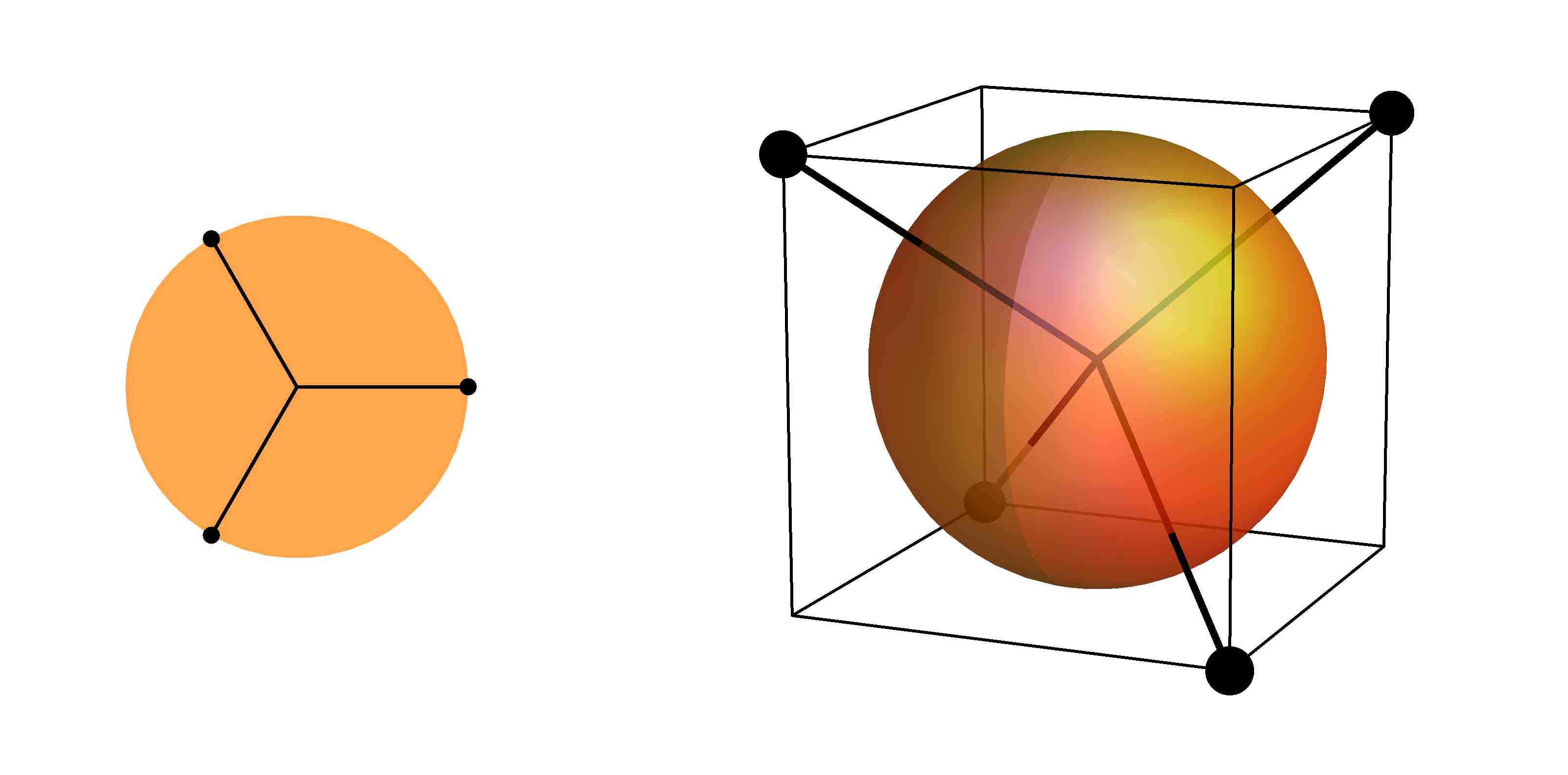
Figure 7: Left: unit disk with three uniformly spaced vectors, the building blocks for the $120^{\circ}$ model with $n=2$, on for instance a $3D$ cubic or the $2D$ honeycomb lattice. Right: generalization to higher dimensions with four uniformly spaced vectors on the $n=3$ dimensional unit sphere, relevant to a $4D$ hyper-cubic lattice, or the $3D$ diamond lattice.

An obvious extension is to consider vectors ${\bm{T}}$ with a general number of components $n$. The $90^{\circ}$ compass models (Eq. (7)) generalize straightforwardly to any system having $n$ independent directions $\gamma$. The simplest variant of this type is a hyper-cubic lattice in $D=n$ dimensions wherein along each axis $\gamma$ (all at 90^∘ relative to each other) the interaction is of the form

$$H_{\square}^{~{}\sf classical~{}90^{\circ}}=-\sum_{i,\gamma}J_{\gamma}T_{i}^{\gamma}T_{i+\hat{e}_{\gamma}}^{\gamma}.$$ (43)

[More generally, we will set in general classical analogs, $T^{\gamma}_{i}\equiv{\bf T}_{i}\cdot{\bf e}_{\gamma}$.] When looked at through this prism, the one dimensional Ising model can be viewed as a classical one dimensional rendition of a compass model.

In the classical arena, when ${\bm{\tau}}$ is replaced by vectors ${\bm{T}}$ of unit norm, there is also a natural generalization of the 120^∘ compass model to hyper-cubic lattices in arbitrary spatial dimension $D$. To formulate this generalization, it is useful to introduce the unit sphere in $n$ dimensions. In the classical 120^∘ compass model on the $D=3$ cubic lattice, the three two-component vectors $T^{\gamma}$ are uniformly partitioned on the unit disk (the $n=2$ unit sphere). These form $D$ equally spaced directions $\bm{e}_{\gamma}$ on the $n$ unit sphere. The angle $\theta$ between any pair of differing vectors is therefore same (and for $n=2$ equal to $2\pi/3$). The generic requirement of uniform angular spacing of $D$ vectors on a sphere in $n$ dimensions is possible only when $n=D-1$. The angle $\theta$ between the unit vectors is then given by

$$\bm{e}_{\gamma}\cdot\bm{e}_{\gamma^{\prime}}=\cos\theta=-\frac{1}{D-1}.$$ (44)

If $n=3$, for instance, the four equally spaced vectors can be used to describe the interactions on any lattice having 4 independent directions $\gamma$, for instance the $4D$ hyper-cubic one, or the $3D$ diamond lattice, see Fig. 7.

It is interesting to note that formally, in the limit of high spatial dimension of a hyper-cubic lattice rendition of the 120^∘ model, the angle $\theta\to$ 90^∘ and the two most prominent types of compass models discussed above (the 90^∘ and 120^∘ compass models) become similar (albeit differing by one dimension of the $n$ dimensional unit sphere on which ${\bm{T}}$ is defined).

From here one can return to the quantum arena. The quantum analogues of these $D$ dimensional classical compass models (including extensions of the 120^∘ model on a $3D$ cubic lattice) can be attained by replacing ${\bm{T}}$ by corresponding quantum operators ${\bm{\tau}}$ that are the generators of spin angular momentum in $n$ dimensional space. These are then finite size representations of the quantum spin angular momentum generators in an $n$ dimensional space (e.g., the representations $T=1/2,1,3/2,...)$ of SU(2) for a three component vector just discussed earlier (including the pertinent $T=1/2$ representation), representations of SU(2) $\times$ SU(2) for a four component ${\bm{\tau}}$, representations of Sp(2) and SU(4) for a five and six component ${\bm{\tau}}$, and so on).

These dimensional extensions and definitions of the 90^∘ and 120^∘ models are not unique. The so-called “one dimensional 90^∘ compass model” (sometimes also referred to as the one-dimensional Kitaev model) was studied in multiple works, e.g., Brzezicki et al. (2007); You & Tian (2008); Sun et al. (2008). In its simplest initial rendition Brzezicki et al. (2007), this model is defined on a chain in which nearest neighbor interactions sequentially toggle between being of the $\tau^{x}_{2i}\tau^{x}_{2i+1}$ and $\tau^{y}_{2i+1}\tau^{y}_{2i+2}$ variants as one proceeds along the chain direction for even/odd numbered bonds. Many aspects of this model have been investigated such as its quench dynamics Divakarian & Dutta (2009); Mondal et al. (2008). Such a system is, in fact, dual to the well-studied one-dimensional transverse field Ising model, e.g., Brzezicki et al. (2007); Nussinov & Ortiz (2009b); Eriksson & Johannesson (2009). A two leg ladder rendition of Kitaev’s honeycomb model (and, in particular, the quench dynamics in this system) was investigated in Sen & Vishveshwara (2010). A very interesting two-dimensional realization of the 120^∘ model was further introduced and studied  You & Tian (2008) wherein only two of the directions $\gamma$ are active in Eq. (27).

Lastly, we comment on these models (in their classical or quantum realization) in the “large $n$ limit” wherein the number of Cartesian components of the pseudo-spins ${\bf T}$ becomes large. This limit, albeit seemingly academic, is special. The $n\to\infty$ limit has the virtue that it is exactly solvable, where it reduces to the “spherical model”, Berlin & Kac (1952); Stanley (1968) and further amenable to perturbative corrections in “$1/n$ expansions” Ma (1973). We will return to discuss some aspects of the large $n$ limit in section VIII.

III.3 Other Extended Compass Models

III.3.1 Arbitrary angle

Several additional extensions of the more standard models have been proposed and studied in various contexts. One of these includes a generalized angle that need not be 90^∘ or 120^∘ or another special value Ref. Cincio et al. (2010) considered a variant of Eq. (19) on the square lattice in which, instead of Eq. (27), one has

$$\hat{\pi}_{i}^{x}=\cos(\theta/2)\tau_{i}^{x}+\sin(\theta/2)\tau_{i}^{y}$$

$$\hat{\pi}_{i}^{y}=\cos(\theta/2)\tau_{i}^{x}-\sin(\theta/2)\tau_{i}^{y}$$ (45)

with a tunable angle $\theta$.

III.3.2 Plaquette and Checkerboard (sub-)lattices

Another variant that has been considered, initially introduced to better enable simulation Wenzel & Janke (2009), is one in which the angle $\theta$ is held fixed ($\theta=90^{\circ}$) but the distribution of various bonds is permuted over the lattice Biskup & Kotecky (2010). Specifically, the plaquette orbital model is defined on the square lattice via

$$H_{POM}=-J_{A}\sum_{\langle ij\rangle\in A}\tau^{x}_{i}\tau^{x}_{j}-J_{B}\sum_{\langle ij\rangle\in B}\tau^{y}_{i}\tau^{y}_{j},$$ (46)

where $A$ and $B$ denote two plaquette sublattices, see Fig. 8. Bonds are summed over according to whether the physical link $\langle ij\rangle$ resides in sublattice A or sublattice B.

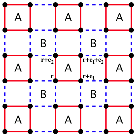
Figure 8: The configuration underlying the definition of the plaquette orbital model. Here the $x$ components of the spins are coupled over the red (solid) edges and the $z$ components are coupled over the blue (dashed) edges Biskup & Kotecky (2010).

Although this system is quite distinct from the models introduced thus far, it does share some common features, including a bond algebra (the notion of bond-algebra Cobanera et al. (2010, 2011); Nussinov & Ortiz (2008c, 2009b) will be introduced and applied to the Kitaev model in subsection X.3) which as the reader may verify in the Appendix (Section XIII)) is, locally, similar to that of the 90^∘ compass model on the square lattice.

The checkerboard lattice (a two-dimensional variant of the three-dimensional pyrochlore lattice) is composed of corner sharing crossed plaquettes. This lattice may be regarded as a square lattice in which on every other square plaquettes, there are additional diagonal links, see Fig. 9.

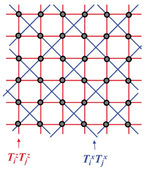
Figure 9: A schematic representation for the orbital compass model on a checkerboard lattice. Nasu et al. (2012a).

On this lattice, a compass model may be defined by the following Hamiltonian Nasu & Ishihara (2011a); Nasu et al. (2012a)

$$H_{checkerboard}=-J_{x}\sum_{(ij)}\tau_{i}^{x}\tau_{j}^{x}-J_{z}\sum_{\langle ij\rangle}\tau^{z}_{i}\tau^{z}_{j}.$$ (47)

In the first term of Eq. (47), the sum is over diagonal (or next nearest neighbor) pairs in crossed plaquettes. The second term in Eq. (47) contains a sum over all nearest neighbor (i.e., horizontal or vertical) pairs on the lattice.

III.3.3 Longer-range and Ring Interactions

In a similar vein, compass models can be defined by pair interactions of varying range and orientation on other general lattices. For instance in the study of layered oxides, Kargarian et al., 2012 introduced a hybrid compass model of Heisenberg-Kitaev type with nearest-neighbor and next-neighbor interactions on the honeycomb lattice, which we will return to in section V.1.8.

One should keep in mind that models in which different spin components couple for different spatial separations may be similar to compass models that we have considered in the previous sections, yet on enlarged lattices. A case in point is that of a one dimensional spin system with the Hamiltonian

$$H_{chain}=-J_{x}\sum_{i}\tau_{i}^{x}\tau_{i+1}^{x}-J_{z}\sum_{i}\tau^{z}_{i}\tau^{z}_{i+2}.$$ (48)

Here, the interactions on the chain defined by the Hamiltonian of Eq. (48) are topologically equivalent to a system composed on two parallel chains that are horizontally displaced from one another by half a lattice constant. On one of these chains, we label the sites by odd integers, i.e., $i=1,3,5,...$ while the other chain hosts the even sites $i=2,4,...$. On this lattice, the Hamiltonian of Eq. (48) assumes a form similar to that of Eq. (47) when the $J_{x}$ interactions appear along diagonally connected sites between the two chains while $J_{z}$ coupling occurs between spins that lie on the same chain. Thus, the one dimensional system with interactions that vary with the range of the coupling between spins is equivalent to a compass model wherein the spin coupling is dependent on the orientation between neighboring spin pairs.

Compass models need not involve only pair interactions. A key feature of models that go beyond pair interactions is that the internal pseudospin components appearing in the interaction terms that depend on a external spatial direction can be extended to any number of interacting pseudospins. A very natural variant was considered in Nasu & Ishihara (2011c) for ring exchange interactions involving four spins around basic square plaquette in a cubic lattice. Specifically, these interactions are defined via the Hamiltonian

$$H_{ring}=K\sum_{[ijkl]_{\gamma}}(\tau^{\gamma+}_{i}\tau^{\gamma-}_{j}\tau^{\gamma+}_{k}\tau^{\gamma-}_{l}+h.c.).$$ (49)

In  Eq.(49), $\tau^{\pm\gamma}_{i}=\tau^{\gamma}_{i}\pm i\frac{\sqrt{3}}{2}\tau^{y}_{i}$ where, similar to the 120^∘ model, $\tau_{i}^{\gamma}=\cos(2\pi n_{\gamma}/3)\tau^{z}_{i}-\sin(2\pi n_{\gamma}/3)\tau_{i}^{x}.$ In Eq. (49), the subscript $[ijkl]_{\gamma}$ denotes sites $[ijkl]$ forming a four-site plaquette that is perpendicular to the cubic lattice direction $\gamma$. In the definition of $\tau_{i}^{\gamma}$, $n_{\gamma}=1$ for a direction $\gamma$ parallel to the x-axis (i.e., the plaquette $[ijkl]$ is orthogonal to the x direction). Similarly, $n_{\gamma}=2$ or 3 for an orientation $\gamma$ parallel to the cubic lattice y- or z- axis. The physically motivated Hamiltonian of Eq.(49) with its definitions of $\tau_{i}^{\gamma}$ corresponds to a ring-exchange of interactions of the 120^∘ type. One may similarly consider extensions for other angles $\theta$.

IV Compass Model Representations

IV.1 Continuum Representation

A standard approach in statistical mechanics is to construct effective continuum descriptions of discrete models. A continuum representation of a compass models can be attained by coarse-graining its discrete counterpart with pseudo-spins attached to each point on a lattice. Such coarse-grained continuum representations can offer much insight into the low-energy, long-wave-length behavior and properties of lattice models. We therefore briefly discuss the particular field-theoretic incarnation of compass type systems, both classical and quantum.

IV.1.1 Classical Compass Models

For a classical pseudospin $\bm{T}$ one defines $T_{i}^{\gamma}=\bm{T}_{i}\cdot\bf{n}_{\gamma},$ with the angles defining $\bf{n}_{\gamma}=(\cos\theta_{\gamma},\sin\theta_{\gamma})$ given by Eq.(27) for the 120^o model. Similarly, in the 90^o compass model in three dimensions, the three internal pseudospin polarization directions ${\bf{n}}$ are defined by ${\bf{n}}={\bf{e}}_{x},{\bf{e}}_{y}$ or ${\bf{e}}_{z}$. In going over from the discrete lattice model to its continuum representation one uses

$$-T_{i}^{\gamma}T_{i+{\bf{e}}_{\gamma}}^{\gamma} \to \frac{a}{2}(T^{\gamma}_{i+{\bf{e}}_{\gamma}}-T_{i}^{\gamma})^{2}-\frac{a}{2}[(T_{i+{\bf{e}}_{\gamma}}^{\gamma})^{2}+(T_{i}^{\gamma})^{2}]$$ (50)

$$\to \frac{a}{2}(\partial_{\gamma}T^{\gamma})^{2},$$

where $a$ is the lattice constant and the normalization of the pseudo-vector $\sum_{\gamma}(T_{i}^{\gamma})^{2}$ has been invoked. Classical compass models will be reviewed in detail later. For now, we note that if $\bm{T}$ is a vector of unit norm then, in the 120⁰ model in $D=3$ dimensions, regardless of the orientation of that vector on the unit disk, $\sum_{\gamma}(T_{i}^{\gamma})^{2}=3/2$ identically. (For a rendition of the 120^o model of the form of Eq. (44) in $D$ dimensions the general result is $D/(D-1)$.) In a similar fashion, for the classical 90^o model $\sum_{\gamma}(T_{i}^{\gamma})^{2}=1$. In all such instances, $\sum_{\gamma}(T_{i}^{\gamma})^{2}$ identically amounts to an innocuous constant and as such may be discarded.

In what follows, briefly the “soft-spin” approximation will be discussed, in which the “hard-spin” constraint ${\bf{T}}^{2}=1$ is replaced by a quartic term of order $\lambda$ that enforces it weakly. Such a term is of the form $(\lambda/4!)({\bf{T}}^{2}-1)^{2}$ with small positive $\lambda$. The limit $\lambda\to\infty$ corresponds to the “hard-spin” situation in which the pseudospin is strictly normalized at every point.

With the definition of $T_{i}^{\gamma}$ and simple preliminaries, the continuum limit Ginzburg-Landau type free energy in $D$ spatial dimensions is

$$F=\int d^{D}x\Big{[}\sum_{\gamma}\frac{(\partial_{\gamma}T^{\gamma})^{2}}{2g}+\frac{r}{2}{\bf{T}}^{2}+\frac{\lambda}{4!}({\bf{T}}^{2})^{2}\Big{]},$$ (51)

with $g$ an inverse coupling constant and $r$ a parameter that emulates the effect of temperature, $r=c(\cal{T}-\cal{T}_{0})$ with $c$ a positive constant and $\cal{T}_{0}$ the mean-field temperature. The partition function of the theory is then given by a functional integration over all pseudospin configurations at all lattice sites, $Z=\int DTe^{-F}$. What differentiates this form from standard field theories is that it does not transform as a simple scalar under rotations. Inspecting Eq. (51), one sees that there is no implicit immediate summation over the repeated index $\gamma$ in the argument of the square. In Eq. (51), the summation over $\gamma$ is performed at the end after the squares of the various gradients have been taken. Written long-hand for, e.g., the 90^o compass model in two dimensions, the integrand is

$$\left(\frac{\partial T^{x}}{\partial x}\right)^{2}+\left(\frac{\partial T^{y}}{\partial y}\right)^{2}.$$ (52)

This is to be distinguished from the square of the divergence of $\bf{T}$ (in which the sum over $\gamma$ would be made prior to taking the square) which would read

$$\left(\frac{\partial T^{x}}{\partial x}\right)^{2}+2\frac{\partial T^{x}}{\partial x}\frac{\partial T^{y}}{\partial y}+\left(\frac{\partial T^{y}}{\partial y}\right)^{2}.$$ (53)

This is also different from the square of the gradient of components $T^{\gamma}$ and their sums thereof for which, rather explicitly, one would have for any single component $\gamma=x$ or $y$,

$$(\nabla T^{\gamma})^{2}=\left(\frac{\partial T^{\gamma}}{\partial x}\right)^{2}+\left(\frac{\partial T^{\gamma}}{\partial y}\right)^{2}.$$ (54)

In the present case, ${\bf{T}}$ indeed represents an internal degree of freedom that does not transform under a rotation of space. By comparison to standard field-theories, Eq. (51) manifestly breaks rotational invariance – a feature that is inherited from the original lattice models that it emulates. In Sec. VI the investigations of symmetries as well as of the classical compass models will be reviewed in detail.

IV.1.2 Quantum Compass Models

As with usual spin models, the quantum pseudospin systems differ from their classical counterparts by the addition of Berry phase terms. This phase, identical in form to that appearing in spin systems, can be written both in the real time and the imaginary time (Euclidean) formalisms. Fradkin (1991); Sachdev (1999) In the quantum arena, one considers the dynamics in imaginary time $\tau$ where $0\leq u\leq\beta$ with $\beta$ the inverse temperature. The pseudospin ${\bf T}(u)$ evolves on a sphere of radius $T$ with the boundary conditions that ${\bf T}(u=0)={\bf T}(u=\beta)$. Thus, the pseudospin describes a closed trajectory on a sphere of radius $T$. The Berry phase for quantum spin systems (also known as the Wess-Zumino-Witten term (WZW)) is, for each single pseudospin at site $j$, given by $S^{WZW}_{j}=-iTA_{j}$ with $A$ the area the spherical cap circumscribed by the closed pseudospin trajectory at that site. That is, there is a quantum mechanical (Aharonov-Bohm type) phase that would be associated with a magnetic monopole of strength $T$ situated at the origin. Denoting the orientation on the unit sphere by ${\bf{n}}$, that monopole may be described by a vector potential ${\cal{A}}$ is a function of ${\bf{n}}$ that solves the equation $\epsilon^{abc}(\partial{\cal{A}}^{b}/\partial n^{c})=Tn^{a}$. The partition function is given by for ferromagnetic variants of the compass models is given by

$$Z = \int Dn^{a}({\bf x},u)\delta((n^{a})^{2}-1)\exp(-S),$$

$$S = iT\int_{0}^{\beta}du\int d^{D}x{\cal{A}}^{a}\frac{dn^{a}}{du}$$ (55)

$$+ T^{2}\int_{0}^{\beta}du\int d^{D}x\sum_{\gamma}\frac{(\partial_{\gamma}n^{\gamma})^{2}}{2g}.$$

As in the classical case, we note that here summation over $\gamma$ is performed only after the squares have been taken. Similar to the “soft-spin” classical model, it is possible to construct approximations in which the delta function in Eq. (55) is replaced by soft quartic potentials of the form $\frac{\lambda}{4!}({\bf n}^{2}-1)^{2}$. In the classical case as well as for XY quantum systems (such as the 120^o compass), the behavior of $J>0$ and $J<0$ systems is identical. As noted earlier, this is no longer true in quantum compass systems in which all three components of the spin appear. Similar to the case of usual quantum spin systems, the role of the Berry phase terms is quite different for ferromagnetic and anti-ferromagnetic renditions of the three component compass models. Although the squared gradient exchange involving ${\bf n}$ can be made similar when looking at the staggered pseudospin on the lattice, the Berry phase term will change upon such staggering and may lead to non-trivial effects.

IV.2 Momentum Space Representations

The directional dependence of the interactions in compass models is, of course, manifest also in momentum space. Such a momentum space representation strongly hint that the 90^o compass models may exhibit a dimensional reduction Batista & Nussinov (2005). A general pseudospin model having $n$ components can be Fourier transformed and cast into the form

$$H=\frac{1}{2}\sum_{\bf k}{\bf T}^{\dagger}({\bf k})\hat{V}({\bf k}){\bf T}({\bf k}).$$ (56)

In Eq. (56), ${\bf k}$ is the momentum space index, the row vector ${\bf T}^{\dagger}({\bf k})=(T^{1}({\bf k}),T^{2}({\bf k}),...,T^{n}({\bf k}))^{*}$ with ^∗ representing complex conjugation is the hermitian conjugate of ${\bf T}({\bf k})$ and ${\hat{V}}({\bf k})$ is a momentum space kernel- an $n\times n$ matrix whose elements depend on the $D$ components of the momenta ${\bf k}$.

In usual isotropic spin exchange systems (i.e., those with isotropic interactions of the form ${\bf T}_{i}\cdot{\bf T}_{j}$ between (real-space) nearest neighbor lattice sites $i$ and $j$), the kernel ${\hat{V}}({\bf k})$ has a particularly simple form,

$${\hat{V}}_{isotropic}=\left(-2\sum_{l=1}^{D}\cos k_{l}\right)\hbox{$1\hskip-1.2pt\vrule depth=0.0pt,height=6.88889pt,width=0.7pt\vrule depth=0.0pt,height=0.3pt,width=1.19995pt$}_{n},$$ (57)

with $k_{l}$ the $l$th Cartesian component of ${\bf k}$ and $\hbox{$1\hskip-1.2pt\vrule depth=0.0pt,height=6.88889pt,width=0.7pt\vrule depth=0.0pt,height=0.3pt,width=1.19995pt$}_{n}$ the $n\times n$ identity matrix. There is a redundancy in the form of Eq. (57) following from spin normalization. At each lattice site $i$ the sum $\sum_{\gamma}(T_{i}^{\gamma})^{2}$ is a constant so that $\sum_{i}(T_{i}^{\gamma})^{2}$ is a constant proportional to the total number of sites. From this follows that $\sum_{\bf{k}}{\bf T}^{\dagger}({\bf k}){\bf{T}}({\bf k})$ is a constant. Consequently, any constant term (i.e., any constant (non-momentum dependent) multiple of the identity matrix) may be added to the right-hand side of Eq. (57). Choosing this constant to be $2D$, in the continuum limit, the right hand of Eq. (57) disperses as ${\bf k}^{2}$ for small wave vectors ${\bf k}$. This is, of course, a manifestation of the usual squared gradient term that appears in standard field theories whose Fourier transform is given by ${\bf k}^{2}$. Thus, in the standard case, the momentum space kernel ${\hat{V}}_{isotropic}$ has a single zero (or lowest energy state) with a dispersion that rises, for small ${\bf{k}}$ quadratically in all directions.

IV.2.1 Dimensional Reduction

The form of the interactions is drastically different for compass models. As will be discussed in e.g., Sec. VIII.2 in greater depth, this may lead to a flat momentum space dispersion in which lines of zeros of ${\hat{V}}({\bf k})$ appear much unlike the typical quadratic dispersion about low energy modes. The relation between the directional character of the interactions in external space (that of $D$ dimensions) and the internal space (the $n$ components of ${\bf T}$). sentences misses verb The $n\times n$ kernel ${\hat{V}}$ can be written down for all of the compass models introduced earlier by replacing any appearance of $(J_{\gamma\gamma^{\prime}l}T^{\gamma}_{i}T^{\gamma^{\prime}}_{j}$) in the Hamiltonian where the real space between nearest neighbor sites $i$ and $j$ are separated along the $l$-th lattice Cartesian direction (on a hypercubic lattice) by a corresponding matrix element of ${\hat{V}}$ that is given by $\langle\gamma|{\hat{V}}|\gamma^{\prime}\rangle=2J_{\gamma\gamma^{\prime}l}\cos k_{l}$. By contrast to the usual isotropic spin exchange interactions, the resulting ${\hat{V}}$ for compass models is no longer an identity matrix in the internal $n$ dimensional space spanning the components of ${\bf T}$. Rather, each component of ${\hat{V}}$ can have a very different dependence on ${\bf k}$. For the 90^o compass models this allows expression of the Hamiltonian in the form of a one-dimensional system in disguise. One sets ${\hat{V}}$ to be a diagonal matrix whose diagonal elements are given by

$$\langle\gamma|{\hat{V}}_{90^{o}}|\gamma\rangle=-2J\cos k_{\gamma},$$ (58)

the 90^o compass model on an $n=D$-dimensional hyper-cubic lattice is recovered. The contrast between Eq. (57) and Eq. (58) is marked and directly captures the directional character of the interactions in the compass model. As in the various compass models (including, trivially, the 90^o compass models), $\sum_{i}(T_{i}^{\gamma})^{2}$ is constant at every lattice site $i$, one may as before add to the right hand side of Eq. (58) any constant times the identity matrix. One can then formally recast Eq. (58) in a form very similar to a one dimensional variant of Eq. (57) – one which depends on only one momentum space “coordinate” but with that coordinate no longer being a $k$ but rather a matrix. Towards that end, one may define a diagonal matrix $\hat{K}$ whose diagonal matrix elements are given by $(k_{1},...,k_{n})$ and cast Eq. (58) as

$${\hat{V}}_{90^{o}}=-2J\cos\hat{K}.$$ (59)

In this form, Eq. (59) looks like a one dimensional $(D=1)$ model by comparison to Eq. (57). The only difference is that instead of having a real scalar quantity $k$ in $1D$ one now formally has an $D\times D$ dimensional matrix (or a quaternion form for the $D=2$ dimensional 90^∘ compass model) but otherwise it looks very much similar.

Indeed, to lowest orders in various approximations ($1/n$, high temperature series expansions, etc.) the 90^o compass models appears to be one dimensional. This is evident in the spin-wave spectrum: naively, to lowest orders in all of these approaches, there seems to be a decoupling of excitations along different directions. That is, in the continuum (small ${\bf k}$ limit), one may replace $2(1-\cos k_{\gamma})$ by $k_{\gamma}^{2}$ and the spectrum for excitations involving $T^{\gamma}$ is identical to that of a one dimensional system parallel to the Cartesian $\gamma$ direction. This is a manifestation of the unusual gradient terms that appear in the continuum representation of the compass model – Eqs. (50,51). In reality, though, the compass models express the character expected from systems in $D$ dimensions (not one-dimensional systems) along their finite temperature phase transitions and universality classes. In the field theory representation of Eq. (51), this occurs due to the quartic term that couples the different pseudospin polarization directions (e.g., $T^{x}$ and $T^{y}$) to one another. However, an exact remnant of the dimensional reduction suggested by this form still persists in the form of symmetries Batista & Nussinov (2005), see Sec. VI.

IV.2.2 (In-)Commensurate Ground States

In what follows below and in later sections, the eigenvalues of ${\bf V}({\bf k})$ for each ${\bf k}$ are denoted by $v_{\alpha}({\bf k})$ with $\alpha=1,2,...,n$ with $n$ the number of pseudo-spin components. In rotationally symmetric, isotropic systems when $v_{\alpha}({\bf k})$ is independent of the pseudo-spin index $\alpha$ and $\pm{\bf q}^{*}$ are two wave-vectors that minimize $v$ then, it is easy to see that two-component spirals of the form ${\bf{T}}({\bf r})=(\cos{\bm{q}^{*}}\cdot{\bm{r}},\sin{\bm{q}^{*}}\cdot{\bm{r}})$ are classical ground states of the normalized pseudo-spins ${\bf T}$. Similar extensions appear for $n=3$ (and higher) component pseudo-spins. It has been proven that for general incommensurate wave-vectors ${\bf q}^{*}$, all ground states must be spirals of this form Nussinov (2001); Nussinov et al. (1999). When the wave-vectors that minimize $v$ are related to one another by commensurability conditions Nussinov (2001) then more complicated (e.g., stripe or checkerboard type) configurations can arise.

In several compass type systems that are reviewed here (e.g., the 90^∘ compass and Kitaev’s honeycomb model), the interaction kernel $v$ will still be diagonal in the original internal pseudo-spin component basis ($\alpha=1,2,\cdots,n$) yet $v_{\alpha}({\bf k})$ will different functions for different $\alpha$. Depending on the model at hand, these functions for different components $\alpha$ may be related to one another by a point group rotation of ${\bf k}$ from one lattice direction to another. We briefly remark on the case when the wave-vectors ${\bf q}^{*}$ that minimize, for each $\alpha$, the kernel $v_{\alpha}({\bf k})$ are commensurate and allow the construction of Ising type ground states Nussinov (2001) such as commensurate stripes or checkerboard states. In such a case it is possible to construct $n$ component ground states by having Ising type states for each component $\alpha$. That is, for each internal spin direction $\alpha=1,2,...,n$, we can construct states with $(T_{\alpha}^{2}=a_{\alpha}^{2}$ with $a_{\alpha}$ (for an Ising system, only one component $n=1$ exists and $a_{\alpha}=1$, for Ising type states, we scale each Cartesian component by a uniform factor of $a_{\alpha}$ at all lattice site and require that $\sum_{\alpha=1}^{n}a_{\alpha}^{2}=1$ to ensure global pseudo-spin normalization. As we will review in later sections, the symmetries that compass type systems exhibit ensures that in many cases there is a multitude of ground states that extends beyond expectations in most other (pseudo)spin systems.

IV.3 Ising Model Representations

It is well-known that using the Feynman mapping, one can relate zero temperature quantum system in $D$ spatial dimensions to classical systems in $(D+1)$ dimensions Sachdev (1999). In the current context, one can express many of the quantum compass systems as classical Ising models in one higher dimension. The key idea of such Feynman maps is to work in a classical Ising basis ($\{\sigma^{z}_{i,u}\}$) at each point in space $i$ and imaginary time $u$ and to write the transfer matrix elements of the imaginary time evolution operator between the system and itself at two temporally separated times. The derivation will not be reviewed here, see e.g., Sachdev (1999).

A simple variant of the Feynman mapping invokes duality considerations Nussinov & Fradkin (2005); Cobanera et al. (2010, 2011) to another quantum system Xu & Moore (2004, 2005) prior to the use of the standard transfer matrix technique. Here we merely quote the results. The two-dimensional 90^o compass model of Eq. (6) in the absence of an external field ($h=0$) maps onto a classical model in 2+1 dimensions with the action Nussinov & Fradkin (2005); Cobanera et al. (2011)

$$S= -K \sum_{\Box\in(xu)~{}{\rm plane}}\sigma^{z}_{i,u}\sigma^{z}_{i+{\bf{e}}_{x},u}\sigma^{z}_{i,u+\Delta u}\sigma^{z}_{i+{\bf{e}}_{x},u+\Delta u}$$ (60)

$$-J_{z}\Delta u\sum_{i}\sigma^{z}_{i,u}\sigma^{z}_{i+{\bf{e}}_{z},u},$$

with $K$ and $J_{z}\Delta u$ constants that will be detailed later on. The Ising spins $\{\sigma^{z}_{i,u}\}$ are situated at lattice points in the 2+1 dimensional lattice in space-time. A particular separation $\Delta u$ along the imaginary time axis has to be specified in performing the mapping of the quantum system onto a classical lattice system in space-time. The coupling constants in Eq. (60) are directly related to those in Eq. (6). We aim to keep the form of Eq. (60) general and cast it in the form of a gauge type theory (with spins at the vertices of the lattice instead of on links). The plaquette coupling $K$ is related to the coupling constant $J_{x}$ of Eq. (6) via

$$\sinh 2(J_{x}\Delta u)\sinh 2K=1.$$ (61)

The particular anisotropic directional character of the compass model rears its head in Eq. (60). Unlike canonical systems in which the form of the interactions is the same in all plaquettes regardless of their orientation, here four-spin interactions appear only for plaquette that lie parallel to the $(xu)$ plane- that is, the plane spanned by one of Cartesian spatial directions ($x$) and the imaginary time axis ($u$). Similarly, exchange interactions (of strength $(J_{z}\Delta u)$) appears between pairs of spins that are separated along links parallel to the spatial Cartesian $z$ direction.

The zero temperature effective classical Ising action of Eq. (60) enables the study of the character of the zero temperature transition that occurs as $J_{x}/J_{z}$ is varied. From the original compass model of Eq. (1), it is clear that when $|J_{z}|$ exceeds $|J_{x}|$ there is a preferential orientation of the spins along the $z$ axis (and, vice versa, when $|J_{x}|$ exceeds $|J_{z}$ an ordering along the $x$ axis is preferred). The point $J_{x}=J_{z}$ (a “self-dual” point for reasons which will be elaborated on later) marks a transition which has been studied by various other beautiful means and found to be first order Dorier et al. (2005); Chen et al. (2007); Orús et al. (2009).

IV.4 Dynamics – Equation of Motion

The anisotropic form of the interactions leads to equations of motion that formally appear similar to those in magnetic systems but are highly anisotropic. In general spin and pseudospin systems, time evolution (both classical (i.e., classical magnetic moments) and quantum) is governed by the equation of motion

$$\frac{\partial{\bf T}_{i}}{\partial t}={\bf T}_{i}\times{\bf h}_{i},$$ (62)

where ${\bf h}_{i}$ is the local magnetic (pseudo-magnetic) field at site $i$. For a stationary field ${\bf h}$, this leads to a ”Larmor precession”- the spin rotates at constant rate about the field direction. This well known spin effect has a simple incarnation for pseudospins where it may further implies a non-trivial time evolution of electronic orbitals Nussinov & Ortiz (2008c) or any other degree of freedom that the pseudospin represents.

For uniform ferromagnetic variants of the compass models (with a single constant $J$), the equation of motion is

$$\frac{\partial{\bf T}_{i}}{\partial t}=J{\bf T}_{i}\times\sum_{j}({\bf T}_{j}\cdot{\bf e}_{\gamma||\langle ij\rangle}){\bf e}_{\gamma||\langle ij\rangle},$$ (63)

which directly follows from Eq. (62). In Eq. (63), the sum is over sites $j$ that are nearest neighbors of $i$. By the designation ${\bf e}_{\gamma||\langle ij\rangle}$, we make explicit that the internal pseudospin direction ${\bf e}_{\gamma}$ is set by that particular value of $\gamma$ that corresponds to the direction from site $i$ to site $j$ on the lattice itself (i.e., by the direction of the lattice link $\langle ij\rangle$). If the effective pseudo-magnetic field at site $i$ is parallel to the pseudospin at that site, $\Big{(}\sum_{j}({\bf T}_{j}\cdot{\bf e}_{\gamma||\langle ij\rangle}){\bf e}_{\gamma||\langle ij\rangle}\Big{)}||{\bf T}_{i}$ then semi-classicaly the pseudospin is stationary (i.e., $\partial{\bf T}_{i}/\partial t=0$). Such a case arises, for instance, for any semi-classical uniform pseudospin configuration: ${\bf T}_{i}$ = constant vector for all $i$ which we denote below by ${\bf T}$. In such a case, for the 90^o compass, $\sum_{j}({\bf T}_{j}\cdot{\bf e}_{\gamma||\langle ij\rangle}){\bf e}_{\gamma||\langle ij\rangle}=2{\bf T}$ whereas for the cubic lattice 120^o compass, $\sum_{j}({\bf T}_{j}\cdot{\bf e}_{\gamma||\langle ij\rangle}){\bf e}_{\gamma||\langle ij\rangle}=3{\bf T}$.

As, classically, ${\bf T}\times{\bf T}=0$, all uniform pseudospin states are stationary states (which correspond to classical ground states at strictly zero temperature). Similarly, of course, a staggered uniform configuration in which ${\bf T}_{i}$ is equal to one constant value (${\bf T}$) on one sublattice and is equal to $(-{\bf T})$ on the other sublattice, will also lead to a stationary state (that of highest energy for $J>0$). Such semi-classical uniform states are also ground states of usual spin ferromagnets. The interesting twist here is that the effective field ${\bf h}_{i}$ is not given by $J\sum_{j}{\bf S}_{j}$ as for usual spin systems but rather by $\sum_{j}({\bf T}_{j}\cdot{\bf e}_{\gamma||\langle ij\rangle}){\bf e}_{\gamma||\langle ij\rangle}$.

V Physical Motivations & Incarnations

In this section we review the different physical contexts that motivate compass models and how they can emerge as low-energy effective models of systems with strongly interacting electrons. There are quite a few classes of materials where the microscopic interactions between electrons are typically described by an extended Hubbard model. Typically such materials contain transition-metal ions. Hubbard-type models incorporate both the hopping of electrons from lattice-site to lattice-site and the Coulomb interaction $U$ between electrons that meet on the same site, typically the transition-metal ion. Particularly in the situation that electron-electron interactions are strong, effective low-energy models can be derived by expanding the Hubbard Hamiltonian in $1/U$ – the inverse interaction strength. In such a low-energy model interactions are not anymore between electrons, but between the remaining spin and orbital degrees of freedom of the electrons.

Compass model Hamiltonians arise, in particular, when orbital degrees of freedom interact with each other, which we will survey in detail (Sec. V.1), but can also emerge in the description of chiral degrees of freedom in frustrated magnets (Sec. V.4).

In the situation that both orbital and spin degrees of freedom are present and their interactions are intertwined, so-called Kugel-Khomskii models arise. We will briefly review in Sec. V.1.4 how such models are relevant for strongly correlated electron systems such as transition metal (TM) oxides, when the low-energy electronic behavior is dominated by the presence of a very strong electron-electron interactions. Within the standard Kugel-Khomskii models, the orbital degrees of freedom are represented via SU(2) type pseudo-spins.

So-called $e_{g}$ and $t_{2g}$ orbital degrees of freedom that can emerge in transition metal compounds with electrons in partially filled TM $d$-shells, give rise to two-flavor compass models (for $e_{g}$) and to three-flavor compass models (for $t_{2g}$) which, as we will explain in this section, are conveniently cast in an SU(3) Gell-Mann matrix form. Precisely these type of compass models emerge in cold atom systems in optical

V.1 Orbital Degrees of Freedom

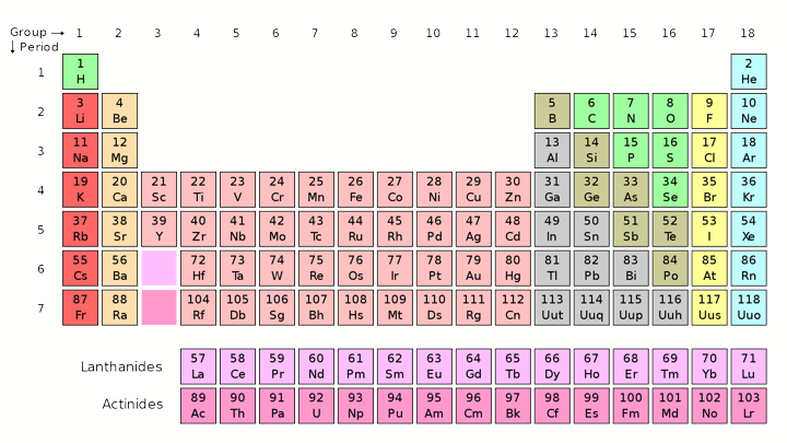
Figure 10: In the periodic table the transition metal (TM) elements with ions that have partially filled $d$-shells are in the 4th row, the $3d$ elements Ti to Cu, below it the $3d$ elements in the 5th row, and the $5d$ elements in the 6th row. Electrons in such partially filled TM $d$-shell can have besides a spin, also an orbital degree of freedom.

Understanding the structure and interplay of orbital degrees of freedom has garnered much attention in various fields. Amongst many others, these include studies of the colossal-magnetoresistance manganites Tokura & Tomioka (1999); van den Brink et al. (2004) and pnictide superconductors Nakayama et al. (2009); Cvetkovic & Tesanovic (2009); Kuroki et al. (2008); Kruger et al. (2009).

Orbital degrees of freedom are already present in the electronic wavefunctions of the hydrogen atom. A brief discussion of the hydrogen atoms with just a single electron can thus serve as a first conceptual introduction to orbital physics (Sec. V.1.1). These concepts translate to transition metal ions, where electrons in partially filled TM $d$-shells can have so-called $e_{g}$ and $t_{2g}$ orbital degrees of freedom Griffith (1971); Fazekas (1999). These orbital states, which can be represented as spinors (Sec. V.1.2), of ions on neighboring lattice sites can interact via electronic superexchange interactions (Sec. V.1.3), which in the most general situation also depends on the spin orientation of the electrons. The relevant Hamiltonians that govern orbital-orbital interactions are derived, and we will briefly review how spin-spin interactions affect the interactions between orbitals in Kugel-Khomskii models (Sec. V.1.4). Reviews on this subject are Refs. Kugel & Khomskii (1982); Tokura & Nagaosa (2000). Sec. V.1.6 is devoted to effective orbital interactions that arise via lattice deformations and give rise to cooperative Jahn-Teller distortions. For $t_{2g}$ orbitals in addition relativistic spin-orbit coupling is relevant, especially for correlated materials build from heavy transition metal ions (those of the 6th row of the periodic table, see Fig. 10), for instance iridates, which will be discussed at the end of this section (Sec. V.1). The basic concepts relevant to strongly correlated electron systems can be found in the books Goodenough (1963); Griffith (1971); Fazekas (1999); Khomskii (2010).

We will first review orbital systems on cubic and other unfrustrated lattices. Caricatures of these systems lead to the most prominent realizations of compass models. It is notable that on frustrated lattices, coupling with the orbital degrees of freedom may lead to rather unconventional states. These include, e.g., on spinel type geometries, spin-orbital molecules in AlV₂O₄ Horibe et al. (2006), a viable cascade of transitions in ZnV₂O₄ Motome & Tsunetsugu (2004). Resonating valence bond states were suggested to occur in the layered triangular compound LiNiO₂ Vernay et al. (2004).

V.1.1 Atomic-like States in Correlated Solids

The well-know hydrogen wave-functions are the product of a radial part $R_{nl}$ and an angular part $Y_{l}^{m}$, with principle quantum number $n$ and angular quantum numbers $l$ and $m$:

$$\psi_{nlm}(r,\theta,\phi) = R_{nl}(2r/n)\cdot Y^{m}_{l}(\theta,\phi),$$ (64)

where the radial coordinate $r$ is measured in Bohr radii, $\theta$, $\phi$ are the angular coordinates and $n$ any positive integer, $l=0,...,n-1$ and $m=-l,...,l$. States with $l=0,1,2,3$ correspond to $s,p,d$ and $f$ states, respectively. The energy levels of hydrogen are $E_{n}=-13.6eV/n^{2}$ when the small spin-orbit coupling is neglected. The energy therefore does not depend on the angular quantum numbers $l$ and $m$, implying that for any $l\geq 1$ the hydrogen energy levels are $2m+1$-fold degenerate – this degeneracy of constitutes the orbital degeneracy and with it the orbital degree of freedom is associated. Thus hydrogen $p$ states are 3-fold degenerate, $d$-states 5-fold and $f$-states 7-fold. In explicit terms the angular wave-functions for the $d$ states, the spherical harmonics $Y_{2}^{m}$ are:

$$Y_{l}^{-m}=(-1)^{m}(Y_{l}^{m})^{*}\ and\left\{\begin{array}[]{l}Y_{2}^{0}=\sqrt{\frac{5}{16\pi}}\left(3\cos^{2}\theta-1\right)\\ Y_{2}^{1}=\sqrt{\frac{15}{8\pi}}\sin\theta\cos\theta e^{i\phi}\\ Y_{2}^{2}=\sqrt{\frac{15}{32\pi}}\sin^{2}\theta e^{i2\phi}\end{array}\right.$$

Introducing the radial coordinates $x=r\sin\theta\cos\phi$, $y=r\sin\theta\sin\phi$ and $z=r\cos\theta$ the angular basis-functions can be combined into real basis-states, for instance $(Y^{-2}_{2}+Y^{2}_{2})/\sqrt{2}=\sqrt{\frac{15}{16\pi}}\sqrt{\frac{1}{r^{2}}}(x^{2}-y^{2})$. Apart from an over-all normalization constant the resulting $d$ orbitals are

$$e_{g}\ orbitals \ \left\{\begin{array}[]{c | l}Y^{-2}_{2}+Y^{2}_{2}&x^{2}-y^{2}\\ \sqrt{2}Y_{2}^{0}&(3z^{2}-r^{2})/\sqrt{3}\end{array}\right.$$

$$t_{2g}\ orbitals \ \left\{\begin{array}[]{c | l}Y^{-2}_{2}-Y^{2}_{2}&xy\\ Y^{-1}_{2}+Y^{1}_{2}&yz\\ Y^{-1}_{2}-Y^{1}_{2}&zx\end{array}\right.$$

where a distinction between so-called $e_{g}$ and $t_{2g}$ orbitals is made, which is based on their different local symmetry properties, as will shortly become clear from crystal field considerations. These orbitals are pictured in Fig. 11. In atoms and ions further down the periodic table (Fig. 10), this orbital degree of freedom can persist, depending on the number of electrons filling a particular electronic shell.

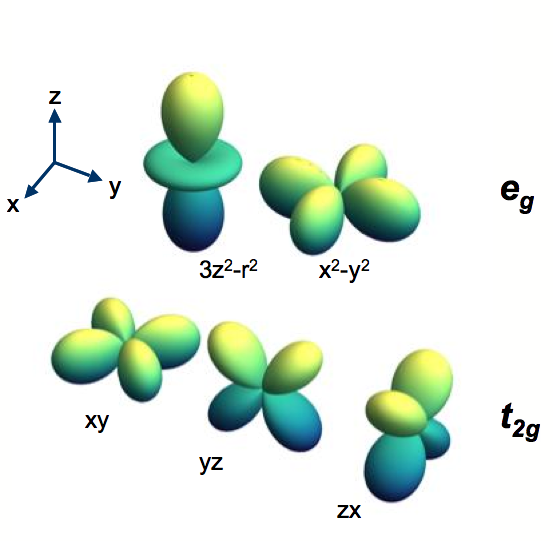
Figure 11: The five orthogonal $d$-orbitals. Crystal field effects lift the five-fold degeneracy of the $d$ atomic orbitals into an $e_{g}$ doublet (top) and a $t_{2g}$ triplet of states.

In solids $p$ wavefunctions of atoms tend to be rather delocalized, forming wide bands. When such wide bands form and a material is consequently a metal or semiconductor, the different atomic states mix and local orbital degeneracies are completely lifted. However, $d$ and $f$ states tend to retain to certain extent their atomic character and especially the $3d$ and $4f$ states are particularly localized – $4d$, $5d$ and $5f$ wave-functions are again more extended than $3d$ and $4f$, respectively. In the periodic table (Fig. 10) ions with open $d$-shells are in the group of transition metals and open $f$-shells are found in the lanthanides and actinides.

The localized nature of $3d$ and $4f$ states has as a consequence that in the solid the interactions between electrons in an open $3d$/$4f$ shell are much like in the atom Griffith (1971). For instance Hund’s first rule – stating that when possible the electrons form high-spin states and maximize their total spin – keeps it relevance for these ions and for the $3d$’s leads to an energy lowering of $J_{H}\sim 0.8$ eV for a pair of electrons having parallel spins. Another large energy scale is the Coulomb interaction $U$ between electrons in the same localized shell. In a solid $U$ is substantially screened from its atomic value and its precise value therefore depends critically on the details of the screening processes – it for instance reduces the Cu d-d Coulomb interactions in copper-oxides from an atomic value of 16 eV to a solid state value of about 5 eV van den Brink et al. (1995). But in many cases it is still the dominant energy scale compared to the bandwidth $W$ of the $3d$ electrons Imada et al. (1998). If $U$ is strong enough, roughly when $U>W$, this causes a collective localization of the electrons and the system becomes a Mott insulator Mott (1990); Fazekas (1999); Khomskii (2010).

In a Mott insulator, that is driven by strong Coulomb interactions, electrons in an open $d$-shell can partially retain their orbital degree of freedom. The full 5-fold degeneracy of the hydrogen-like $d$ states is broken down by the fact that in a solid a positively charged TM ion is surrounded by other ions, which manifestly breaks the rotational invariance that is present in a free hydrogen atom and on the basis of which the atomic wave-functions were derived in the first place. How precisely the 5-fold degeneracy is broken depends on the point group symmetry of the lattice Ballhausen (1962); Fazekas (1999).

The simplest – and rather common – case is the one of cubic symmetry, in which a TM ion is in the center of a cube, with ligand ions at the center of each of its six faces. The negatively charged ligand ions produce an electrical field at the center of the cube. Expanding this field in its multipoles, the first non-vanishing contribution is quadrupolar. This quadrupole field splits the $d$ states into the two $e_{g}$’s and the three $t_{2g}$’s, where the $t_{2g}$’s are lower in energy because the lobes of their electronic wavefunctions point away from the negatively ligand ions Ballhausen (1962); Fazekas (1999), see Fig. 11. Also, the electronic hybridization of these two classes of states with the ligand states is different, which further adds to the energy splitting between the $e_{g}$’s and $t_{2g}$’s. But for a cubic ligand field (also referred to as crystal field) a two-fold orbital degeneracy remains if their is an electron (or a hole) in the $e_{g}$ orbitals and a three-fold degeneracy for an electron/hole in the $t_{2g}$ orbitals.

The two $e_{g}$ states and the three $t_{2g}$ states relate, respectively, to two- and three-dimensional vector spaces (or two- and three-component pseudo-vectors ${\bf T}$). This, combined with the real space anisotropic directional character of the orbitals leads to Hamiltonians similar to compass models that we introduced in earlier sections.

A further lowering of the lattice point-group symmetry, from for instance cubic to tetragonal, will cause a further splitting of degeneracies. The existence of degenerate orbital freedom raises the specter of cooperative effects- i.e., orbital ordering. Indeed, in many of the materials in which they occur, orbital orders appear at high temperatures- often at temperatures far higher than magnetic orders.

V.1.2 Representations of Orbital States

For the $e_{g}$ doublet the orbital pseudospin can be represented by a spinor, where $1\choose 0$ corresponds to an electron in the $x^{2}-y^{2}$ orbital and $0\choose 1$ to the electron in the $(3z^{2}-r^{2})/\sqrt{3}$ orbital. It is instructive to consider the rotations of this spinor, which are generated by the Pauli matrices $\sigma_{1}$, $\sigma_{2}$ and $\sigma_{3}$, the generators of the SU(2) algebra; the identity matrix is $\sigma_{0}$. Rotation by an angle $\phi$ around the $2$-axis is denoted by the operator $\hat{R_{2}}(\phi)$, where

$$\hat{R_{2}}(\phi)=e^{i\sigma_{2}\phi/2}=\sigma_{0}\cos\phi/2+i\sigma_{2}\sin\phi/2.$$ (73)

It is easily checked that for $\phi/2=\pm 2\pi/3$, rotation of the spinor corresponding to $x^{2}-y^{2}$ leads to $\hat{R_{2}^{\pm}}{1\choose 0}=-{1\over 2}{1\choose\mp\sqrt{3}}=-{1\over 2}(x^{2}-y^{2}\mp(3z^{2}-r^{2}))=y^{2}-z^{2},z^{2}-x^{2}$ and similarly $3z^{2}-r^{2}\rightarrow 3x^{2}-r^{2},3y^{2}-r^{2}$. Rotations of the orbital wavefunction by $\phi/2=2\pi/3$, thus cause the successive cyclic permutations $xyz\rightarrow yzx\rightarrow zxy\rightarrow xyz$ in the wavefunctions, as is depicted in Fig. 12.

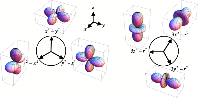
Figure 12: Result of the rotations of the $e_{g}$ orbital spinor by an angle $\phi/2=2\pi/3$.

Next we consider how the pseudospin operator ${\bm{\tau}}$ transforms under these rotations van den Brink et al. (1999a). As ${\bm{\tau}}=\frac{1}{2}\sum_{\alpha\beta}c^{\dagger}_{\alpha}{\bm{\sigma}}_{\alpha\beta}c_{\beta}$, where the sum if over the two different orbital states for each $\alpha$ and $\beta$, after the rotation it is ${\bm{\tau}}=\frac{1}{2}\sum_{\alpha\beta}c^{\dagger}_{\alpha}\hat{R}_{2}^{\mp}{\bm{\sigma}}_{\alpha\beta}\hat{R}^{\pm}_{2}c_{\beta}$. For the vector component $\tau^{3}$ this implies for instance that successive rotations by an angle $\phi/2=\pm 2\pi/3$ transform it as $\tau^{3}\rightarrow-\frac{1}{2}(\tau^{3}+\sqrt{3}\tau^{1})\rightarrow-\frac{1}{2}(\tau^{3}-\sqrt{3}\tau^{1})\rightarrow\tau^{3}$.

The same procedure can be applied to the three $t_{2g}$ states, with can be represented by three-component spinors $xy=\bigl{(}\begin{smallmatrix}1\\ 0\\ 0\end{smallmatrix}\bigr{)}$, $yz=\bigl{(}\begin{smallmatrix}0\\ 1\\ 0\end{smallmatrix}\bigr{)}$ and $zx=\bigl{(}\begin{smallmatrix}0\\ 0\\ 1\end{smallmatrix}\bigr{)}$. The operators acting on the three-flavor spinors form a SU(3) algebra, which is generated by the eight Gell-Mann matrices $\lambda^{1...8}$, see Appendix XIV. This implies that pseudospin operator for $t_{2g}$ orbitals ${\bm{\tau}}=\frac{1}{2}\sum_{\alpha\beta}c^{\dagger}_{\alpha}{\bm{\lambda}}_{\alpha\beta}c_{\beta}$ is an eight-component vector. The operator $\hat{R}^{+}=\bigl{(}\begin{smallmatrix}0&0&1\\ 1&0&0\\ 0&1&0\end{smallmatrix}\bigr{)}$ brings about the cyclic permutations $xyz\rightarrow yzx\rightarrow zxy\rightarrow xyz$ in the $t_{2g}$ wavefunctions and $\hat{R}^{-}=(\hat{R}^{+})^{T}$. $\hat{R}^{\pm}$ applied to the Gell-Man matrices transforms the $t_{2g}$ pseudospin operators accordingly.

V.1.3 Orbital-Orbital Interactions

Figure 13: Superexchange between spin $1/2$ electrons, resulting into the effective antiferromagnetic Heisenberg Hamiltonian $H=J\sum_{i,j}\left({\bf S}_{i}\cdot{\bf S}_{j}-\frac{1}{4}\right)$, with $J=4t^{2}/U$

Even if in a Mott insulator electrons are localized in their atomic-like orbitals, they are not completely confined and can hop between neighboring sites. For electrons in non-degenerate $s$-like orbitals, this lead to the magnetic superexchange interactions between the spins of different electrons, see Fig. 13. The competition between the strong Coulomb interaction that electrons experience when they are in the same orbital, which tends to localize electrons, and the hopping, which tends to delocalize them is captured by the isotropic Hubbard Hamiltonian Hubbard (1963)

$$H^{iso}_{Hub}=\sum_{\begin{subarray}{c}\langle ij\rangle,\alpha=\uparrow,\downarrow\end{subarray}}t(c^{\dagger}_{i\alpha}c^{\phantom{\dagger}}_{j\alpha}+h.c.)+U\sum_{i}n_{i\uparrow}n_{i\downarrow},$$ (74)

where $c^{\dagger}_{i\alpha}$ creates and electron with spin $\alpha=\uparrow,\downarrow$ on site $i$ and $c^{\phantom{\dagger}}_{j\alpha}$ annihilates it on neighboring site $j$, $t$ is the hopping amplitude and the Hubbard $U$ the energy penalty when two electrons meet on the same site and thus are in the same $s$-like orbital Fazekas (1999); Khomskii (2010).

It is convenient to introduce here for later purposes the two by two hopping matrix $t^{\gamma}_{\alpha\beta}$, where with spin $\alpha=\uparrow,\downarrow$ and $\beta=\uparrow,\downarrow$, which determines how an electron changes its spin from $\alpha$ to $\beta$ when it hops from site $i$ to $j$ on the bond $\langle ij\rangle$ in the direction $\gamma$. Using this notation the first term in the Hubbard Hamiltonian $H_{Hub}$ is

$$\sum_{\begin{subarray}{c}\langle ij\rangle,\alpha\end{subarray}}tc^{\dagger}_{i\alpha}c^{\phantom{\dagger}}_{j\alpha}=\sum_{\begin{subarray}{c}i,\gamma,\alpha,\beta\end{subarray}}t^{\gamma}_{\alpha,\beta}c^{\dagger}_{i\alpha}c^{\phantom{\dagger}}_{i+{\bm{e}}_{\gamma}\beta},$$ (75)

so that

$$H_{Hub}=\sum_{\begin{subarray}{c}i,\gamma,\sigma,\sigma\prime\end{subarray}}(t^{\gamma}_{\alpha\beta}c^{\dagger}_{i\alpha}c^{\phantom{\dagger}}_{i+{\bm{e}}_{\gamma}\beta}+h.c.)+U\sum_{\begin{subarray}{c}i\end{subarray}}n_{i\uparrow}n_{i\downarrow},$$ (76)

where for the isotropic Hubbard Hamiltonian $H^{iso}_{Hub}$ of Eq. (76), since hopping does not depend on the direction $\gamma$ of the bond and spin is conserved during the hopping process, we simply have

$$t^{\gamma}_{\alpha\beta}=t\left(\begin{matrix}1&0\\ 0&1\end{matrix}\right),$$ (77)

for all $\gamma$. Compass and Kitaev models are related to Hubbard models with more involved, bond direction depend, forms of $t^{\gamma}_{\alpha\beta}$.

For $U\gg t$ and half filling (i.e. the number of electrons equal to the number of sites in the system) the resulting Heisenberg-type interaction between spins is $H=J\sum_{i,j}\left({\bf S}_{i}\cdot{\bf S}_{j}-\frac{1}{4}\right)$, which is antiferomagnetic: $J=4t^{2}/U$. The high symmetry of the Heisenberg Hamiltonian – the interaction ${\bf S}_{i}\cdot{\bf S}_{j}$ is rotationally invariant – is rooted in the fact that the hopping amplitude $t$ is equal for spin up and spin down electrons and thus does not depend on spin at all. This is again reflected by the hopping matrix of an electron on site $i$ and spin $\alpha$ to site $j$ and spin $\beta$ being diagonal: $t_{\alpha\beta}=t\bigl{(}\begin{smallmatrix}1&0\\ 0&1\end{smallmatrix}\bigr{)}$. For orbital degrees of freedom the situation is very different, because hopping amplitudes strongly depend on the type of orbitals involved and thus on the orbital pseudospin. This anisotropy is rather extreme as it not only depends on the local symmetry of the two orbitals involved, but also on their relative position in the lattice: for instance the hopping amplitude between two $3z^{2}-r^{2}$ orbitals is very different when the two sites are positioned above each other, along the $z$-axis, or next to each other, e.g. on the $x$-axis, see Fig. 14.

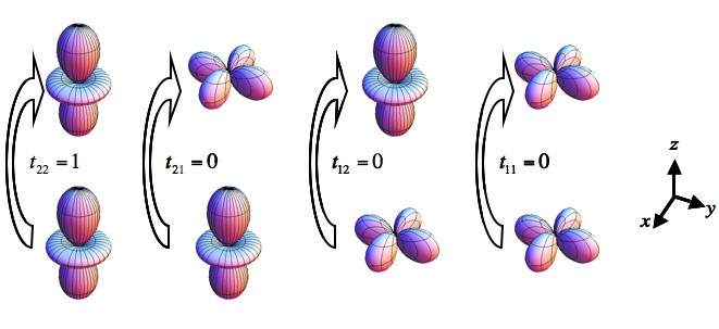
Figure 14: Hopping amplitudes between $e_{g}$ orbitals along the $\hat{z}$ axis: the hopping matrix is $t^{\hat{z}}_{\alpha\beta}=t\delta_{\alpha,2}\delta_{\beta,2}$. Three matrix elements vanish because of the symmetry of the $x^{2}-y^{2}$ orbitals, with a wavefunction on adjacent lobes that has opposite sign.

$e_{g}$ orbital-only Hamiltonians
For the $e_{g}$ orbitals the hopping matrix between sites $i$ and $j$ along the $\hat{z}$ direction is $t_{\alpha\beta}^{\hat{z}}=t\delta_{\alpha,2}\delta_{\beta,2}=t\bigl{(}\begin{smallmatrix}0&0\\ 0&1\end{smallmatrix}\bigr{)}$ in the basis $x^{2}-y^{2}$, $3z^{2}-r^{2}$. This fully species the hopping between orbitals on a cubic lattice, as the hopping along $\hat{x}$ and $\hat{y}$ are dictated by symmetry. The corresponding hopping matrices can be determined with the help of the rotations introduced in the previous subsection, Sec. V.1.2. The hopping matrix $t_{\alpha\beta}^{\hat{x}}$, is obtained by first the full coordinate system is rotated by $\pi/2$ around the $y$-axis, so that $t_{\alpha\beta}^{\hat{z}}\rightarrow t^{\hat{x}}_{\alpha\beta}=t\delta_{\alpha,2}\delta_{\beta,2}$, now with basis states $z^{2}-y^{2}$, $3x^{2}-r^{2}$. A subsequent rotation of the orbital spinors by $\phi/2=-2\pi/3$ around the $2$-axis brings the matrix back in the original $x^{2}-y^{2}$, $3z^{2}-r^{2}$ basis and transforms $t_{\alpha\beta}^{\hat{x}}\rightarrow R_{2}^{+}t_{\alpha\beta}^{\hat{x}}R_{2}^{-}$. After the rotations one finds $t_{\alpha\beta}^{\hat{x}}=\frac{t}{4}\bigl{(}\begin{smallmatrix}3&\sqrt{3}\\ \sqrt{3}&1\end{smallmatrix}\bigr{)}$ and similarly first rotating around the $\hat{y}$-axis and transforming $t_{\alpha\beta}^{\hat{y}}\rightarrow R_{2}^{-}t_{\alpha\beta}^{\hat{x}}R_{2}^{+}$, leads to $t_{\alpha\beta}^{\hat{y}}=\frac{t}{4}\bigl{(}\begin{smallmatrix}3&-\sqrt{3}\\ -\sqrt{3}&1\end{smallmatrix}\bigr{)}$, a well-known result Kugel & Khomskii (1982); van den Brink & Khomskii (1999); Ederer et al. (2007) that is in accordance with microscopic tightbinding considerations Harrison (2004).

Orbital-orbital interactions are generated by superexchange processes between electrons in $e_{g}$ orbitals. When the electron spin is disregarded, the most basic form of the orbital-orbital interaction Hamiltonian is obtained. Superexchange with spin-full electrons leads to Kugel-Khomskii Hamiltonians which will be derived and discussed in the following section. For spin-less fermions the exchange interactions along the $\hat{z}$ axis take a particularly simple form. If the electron on site $i$ is in an $x^{2}-y^{2}$ orbital, corresponding to $\tau_{i}^{3}=-\frac{1}{2}$, and the one on site $j$ in a $3z^{2}-r^{2}$ orbital ($\tau_{j}^{3}=\frac{1}{2}$) a virtual hopping process is possible, giving rise to an energy gain of $-t^{2}/U$ in second order perturbation theory, where $U$ is the energy penalty of having to spinless fermions on the same site (which are by definition in different orbitals). The only other configuration with non-zero energy gain is the one with $i$ and $j$ interchanged. The Hamiltonian on the bond $ij$ is therefore $H^{\hat{z}}_{ij}=-\frac{t^{2}}{U}\left[(\frac{1}{2}-\tau^{3}_{i})(\frac{1}{2}+\tau^{3}_{j})+(\frac{1}{2}-\tau^{3}_{j})(\frac{1}{2}+\tau^{3}_{i})\right]=\frac{J}{2}(\tau^{3}_{i}\tau^{3}_{j}-\frac{1}{4})$. With the same rotations as above, but now acting on the operator $\tau^{z}$, the Hamiltonian on the bonds in the other two directions can be determined: along the $\hat{x}$ and $\hat{y}$ axis, respectively

$$\tau^{3}\rightarrow R_{2}^{+}\tau^{3}R_{2}^{-}\ {\rm along}\ \hat{x}$$

$$\tau^{3}\rightarrow R_{2}^{-}\tau^{3}R_{2}^{+}\ {\rm along}\ \hat{y}$$ (78)

so that $H^{\hat{x}}_{ij}=\frac{J}{8}[(\tau^{3}_{i}+\sqrt{3}\tau^{1}_{i})(\tau^{3}_{j}+\sqrt{3}\tau^{1}_{j})-1]=\frac{J}{4}\pi^{x}_{i}\pi^{x}_{j}$, where the last step defines $\pi^{\gamma}$, (see Eq. (82)) similarly as in Eq. (23), and along $\hat{y}$ one obtains $H^{\hat{y}}_{ij}=\frac{J}{8}[(\tau^{3}_{i}-\sqrt{3}\tau^{1}_{i})(\tau^{3}_{j}-\sqrt{3}\tau^{1}_{j})-1]=\frac{J}{4}\pi^{y}_{i}\pi^{y}_{j}$. The orbital-only Hamiltonian for $e_{g}$ orbital pseudospins therefore is exactly the 120^∘ compass model of Eqs.(19, 23) van den Brink et al. (1999a)

$$H^{e_{g}}_{3\square} = \frac{J}{2}\sum_{i,\gamma}\left(\pi^{\gamma}_{i}\pi^{\gamma}_{i+\bm{e}_{\gamma}}-\frac{1}{4}\right)$$ (82)

$$with\left\{\begin{array}[]{l}\pi^{\gamma}=\tau^{3}\cos{\theta_{\gamma}}+\tau^{1}\sin{\theta_{\gamma}}\\ \{\bm{e}_{\gamma}\}=\{\bm{e}_{x},\bm{e}_{y},\bm{e}_{z}\}\\ \{\theta_{\gamma}\}=\{0,2\pi/3,4\pi/3\}.\end{array}\right.$$

with $J=4t^{2}/U$, which is the 120^∘ quantum compass model on a cubic lattice, Eq. (82), with ”antiferro” orbital-orbital interactions, driving a tendency towards the formation of staggered orbital ordering patterns.

The 120^∘ compass model on the honeycomb lattice $H_{\varhexagon}^{120^{\circ}}$, Eq. (31), was motivated by Nasu et al. (2008) in a study of the layered iron oxides $R$Fe₂O₄ ($R$=Lu, Y, Yb), see Fig. 15. These oxides are multiferroic systems in which both the magnetic and electric response are dominated by Fe $3d$ electrons. The nominal valence of the Fe ions is 2.5 ⁺ and thus an equal number of Fe²⁺ and Fe⁺³ are present. One of the $e_{g}$ levels in the Fe²⁺ ions is doubly occupied where all of the five 3d orbitals in the Fe³⁺ ions are singly occupied. The system assumes the form of a stack of pairs of triangular lattice planes along the $c$ axis of the form Fe²⁺-2Fe³⁺ and 2Fe²⁺-Fe³⁺. In the 2Fe²⁺-Fe³⁺ member of this pair, Fe²⁺ ions (with a doubly degenerate $e_{g}$ orbital degree of freedom) form a honeycomb lattice. Superexchange with the Fe³⁺ ions leads to directly the Hamiltonian of Eq. (31).

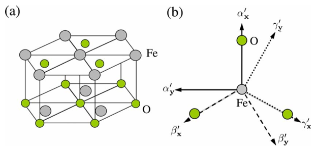
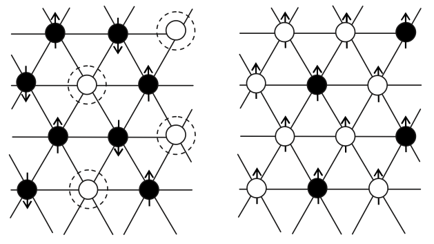
Figure 15: $H_{\varhexagon}^{120^{\circ}}$ models orbital-orbital interactions in RFe₂O₄ (a) A pair of triangular planes and (b) three Fe-O bond directions in a triangular lattice in RFe₂O₄. Nasu et al. (2008). Below: Schematic of the charge and spin structures in 2Fe²⁺-Fe³⁺ plane (right) and in Fe²⁺-2Fe³⁺ plane (left) for RFe₂O₄. Filled and open circles represent Fe³⁺ and Fe²⁺, respectively. At sites surrounded by dotted circles, spin directions are not uniquely determined due to frustration.

The 120^∘ model has been proposed to account for the physics of materials such as NaNiO₂ in which the transition metal ions [with doubly degenerate $e_{g}$ orbitals occupied by a single electron or hole] lie on weakly coupled triangular layers Mostovoy & Khomskii (2002). In NaNiO₂, Na and Ni ions occupy alternate [111] planes as seen in Fig. (16).

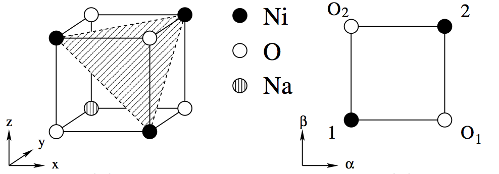
Figure 16: Left: the crystal structure of NaNiO₂. Right: a plaquette in the $\alpha\beta$ plane $(\alpha,\beta=x,y,z)$ formed by two nearest-neighbor Ni ions, 1 and 2, and two oxygens, O₁ and O₂ Mostovoy & Khomskii (2002)

In NaNiO₂, consecutive low spin $Ni^{3+}$ triangular layers are weakly coupled to each other. Within each such layer the dominant interactions between Ni ions involve exchange paths via intermediate oxygens. The bonds between neighboring Ni and oxygen ions form a 90^∘ angle. Direct calculations lead to the triangular lattice 120^∘ Hamiltonian of Eq. (37). In section V.1.7, we will further review charge transfer via intermediate ligand (e.g., oxygen) sites and how they may lead to orbital interactions. Augmenting the orbital only interactions of the 120^∘ compass type, an additional orbital dependent ferromagnetic spin exchange is found Mostovoy & Khomskii (2002). Although the strength of this coupled spin and orbital Hamiltonian varies with the orbital state, the (ferromagnetic) sign of the spin exchange is independent of the orbital configuration; even if the orbitals are in a disordered state, ferromagnetic spin coupling will be present. The spin exchange coupling is far weaker than associated with the orbital interactions (governed by Eq. (37). The experimentally far lower value of the spin ordering temperature is indeed consistent with this analysis Mostovoy & Khomskii (2002) . The dominant interactions are those of the orbital-orbital type.

Compass and Kitaev Hamiltonians
Compass and Kitaev Hamiltonians are the low-energy effective description of certain two-flavor Hubbard Hamiltonians of the type $H_{Hub}$ given by Eq. (76). When the two flavors are spin up and down, the hopping matrix corresponds to the one of the simple isotropic Hubbard model $H^{iso}_{Hub}$, see Eqs.(75,77) and the low-energy effective spin Hamiltonian is the spin 1/2 Heisenberg model. Instead the hopping matrix $t^{\hat{z}}_{\alpha\beta}=\bigl{(}\begin{smallmatrix}0&0\\ 0&1\end{smallmatrix}\bigr{)}$, as for $e_{g}$ orbitals along $\hat{z}$, gives rise to a Ising type of interaction $\tau^{3}_{i}\tau^{3}_{j}$ between pseudospins on the bond $\langle ij\rangle$ parallel to $\hat{z}$. Such a hopping matrix is realized in the original Hubbard model (Eq. 76), if only spin $\downarrow$ electrons would be permitted to hop between the sites $i$ and $j$.

When the hopping matrix has a different form along different bonds a compass model can arises. The 90^∘ compass model, for instance, has a Ising-type interaction $\tau^{3}_{i}\tau^{3}_{j}$ along $\hat{z}$, corresponding to $t^{\hat{z}}_{\alpha\beta}=\bigl{(}\begin{smallmatrix}0&0\\ 0&1\end{smallmatrix}\bigr{)}$, but on the bond along $\hat{x}$ $\tau^{1}_{i}\tau^{1}_{j}$ has to be active, which implies a rotation of (pseudo)spin with angle $\phi=\pi/2$ around the 2-axis, where in the rotated basis the hopping matrix again takes the shape $\bigl{(}\begin{smallmatrix}0&0\\ 0&1\end{smallmatrix}\bigr{)}$. This requires an specific form of the original, unrotated hopping matrix $t_{\alpha\beta}$ along $\hat{x}$. It is easy to check by performing these rotations that for $t^{\hat{x}}_{\alpha\beta}=\frac{1}{2}\bigl{(}\begin{smallmatrix}1&-1\\ -1&1\end{smallmatrix}\bigr{)}$ and $t^{\hat{y}}_{\alpha\beta}=\frac{1}{2}\bigl{(}\begin{smallmatrix}1&-i\\ i&1\end{smallmatrix}\bigr{)}$ the cubic 90^∘ compass model $H_{3\square}^{90^{\circ}}$ (Eq. (8)) arises.

It thus follows that for hopping matrices in the Hubbard Hamiltonian (Eq. (76)) that have the form

$$t^{\hat{x}}_{\alpha,\beta}=\frac{1-\sigma^{x}}{2},\ \ t^{\hat{y}}_{\alpha,\beta}=\frac{1-\sigma^{y}}{2}\ {\rm and}\ t^{\hat{z}}_{\alpha,\beta}=\frac{1-\sigma^{z}}{2}$$ (83)

on a cubic lattice in the large $U$ limit and at half-filling, the low energy effective Hamiltonian is the 90^∘ compass model $H_{3\square}^{90^{\circ}}$ (Eq. (8)). A hopping matrix of this type can be realized physically for electrons in the 5d states of iridium ions, where a strong relativistic spin-orbit coupling locks to spin to the orbital degree of freedom Jackeli & Khaliullin (2009). Controlling the (pseudo)spin dependence of the hopping amplitudes on different bonds thus suffices to generate any type of compass Hamiltonian as the effective low-energy (pseudo)spin model of the Hubbard Hamiltonian.

$t_{2g}$ orbital-only Hamiltonian
The three flavors of $t_{2g}$ orbitals $xy$, $yz$, $zx$ are most naturally represented by a three-component spinor so that the hopping $t_{\alpha\beta}$ is a 3x3 matrix. The structure of the hopping matrix is rather simple (Fig. 17), as between site $i$ and $j$ electrons can only hop between orbitals of the same symmetry so that orbital-flavor is conserved in the hopping process, which renders $t_{\alpha\beta}$ diagonal. Moreover, along the $\hat{x}$ axis the hopping between $yz$ orbitals vanishes. This determines the hopping matrices in all three directions, which can be constructed via rotations, similar as for the $e_{g}$’s, (see Appendix, Sec. XIV):

$$t^{\hat{x}}=\begin{pmatrix}1&0&0\\ 0&0&0\\ 0&0&1\end{pmatrix};\ t^{\hat{y}}=\begin{pmatrix}1&0&0\\ 0&1&0\\ 0&0&0\end{pmatrix};\ t^{\hat{z}}=\begin{pmatrix}0&0&0\\ 0&1&0\\ 0&0&1\end{pmatrix}.$$ (84)

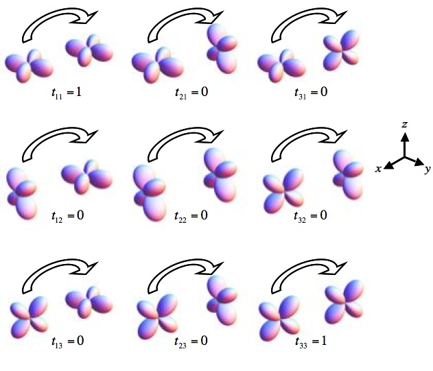
Figure 17: Hopping amplitudes between $t_{2g}$ orbitals along the $\hat{x}$ axis, assuming that the hopping is via an ligand intermediate $p$ state (not shown here), for instance of an oxygen atom between two TM ions, see Figs. 20 and 31.

As along, for instance, the $\hat{y}$ the hopping matrix is diagonal for the two orbitals involved, the exchange interaction for two (spin-less) fermions in these two active orbitals on site $i$ and $j$ is of Heisenberg type. In terms of Gell-Mann matrices it is $\frac{J}{4}(\lambda_{1,i}\lambda_{1,j}+\lambda_{2,i}\lambda_{2,j}+\lambda_{3,i}\lambda_{3,j}-1)$, which is SU(2) invariant. Because both fermions need not be in the two active orbitals, an additional diagonal term $\rho_{1,i}\rho_{1,j}$ is present, where $\rho_{1}=\frac{1}{3}(\lambda_{0}-\sqrt{3}\lambda_{8}$). As $\rho_{1}$ commutes with $\lambda_{1...3}$, it does not break the SU(2) invariance. Defining the vector ${\bm{\mu}}^{1}=(\lambda_{1},\lambda_{2},\lambda_{3},\rho_{1})$ along the $\hat{x}$ direction $H^{\hat{x}}_{ij}=\frac{J}{4}({\bm{\mu}}^{1}_{i}\cdot{\bm{\mu}}^{1}_{j}-1)$. Rotation of the coordinate system and subsequently of the orbital basis produce the interactions along the other two directions, ${\bm{\mu}}^{2}_{i}\cdot{\bm{\mu}}^{2}_{j}-1$ along $\hat{y}$ and ${\bm{\mu}}^{3}_{i}\cdot{\bm{\mu}}^{3}_{j}-1$ along $\hat{z}$, so that

$$H^{t_{2g}}_{3\square} = \frac{J}{4}\sum_{i,\gamma}\left({\bm{\mu}}^{\gamma}_{i}{\bm{\mu}}^{\gamma}_{i+\bm{e}_{\gamma}}-1\right)$$ (85)

with $\{\bm{e}_{\gamma}\}=\{\bm{e}_{x},\bm{e}_{y},\bm{e}_{z}\}$. Along each of the bonds one of the SU(2) subgroups corresponding to the elements of ${\bm{\mu}}^{\gamma}$ is active and the Hamiltonian is rotational invariant in terms of that subgroup. This aspect emphasizes the compass character of the ensuing Hamiltonian. The situation is complicated by the fact that all three ${\bm{\mu}}^{\gamma}$ belong to the same SU(3) algebra, so that the elements of ${\bm{\mu}}^{\gamma}$ and ${\bm{\mu}}^{\gamma^{\prime}}$ in general do not commute.

As the 3-flavor exchange Hamiltonian is represented Gell-Mann matrices, it is natural to refer to it as a Gell-Mann matrix model. This approach allows for a representation of the interactions between $t_{2g}$ orbitals that goes beyond the current well studied orbital Hamiltonians in which SU(2) representations are used. In the context of ultracold gas systems such a number of this type of models has been proposed. Of course the Gell-Mann representation is not unique. Gell-Mann matrices can for example be expressed in polynomials of the three $L=1$ angular momentum matrices $L_{x}$, $L_{y}$ and $L_{z}$, which thus also can be used to represent $H^{t_{2g}}_{3\square}$ Kugel & Khomskii (1982).

V.1.4 Spin-spin and orbital-orbital interactions

Going beyond the case of spin-less fermions, requires considering the local Coulomb and exchange interactions between electrons in various orbital configurations, via a multi-orbital Hubbard Hamiltonian. This opens an entire field, of which reviews can be found in Kugel & Khomskii (1982); Tokura & Nagaosa (2000); Khaliullin (2005b). Here we restrict ourselves to indicating how compass models are decorated with spin-spin interactions, with a particular focus the $120^{\circ}$ compass model for $e_{g}$ electrons.

The considerations concerning the hopping amplitudes of $e_{g}$ electrons directly enter into the kinetic part of the $e_{g}$-orbital Hamiltonian

$$H^{multi}_{Hub} = \sum_{\begin{subarray}{c}i,\gamma\\ \alpha,\beta,\sigma\end{subarray}}t^{\gamma}_{\alpha\beta}(c^{\dagger}_{i,\alpha\sigma}c^{\phantom{\dagger}}_{i+{\bf e}_{\gamma},\beta\sigma}+h.c.)+H_{C}$$ (86)

$${\rm with} \left\{\begin{array}[]{l}t^{\gamma}_{\alpha\beta}=\frac{t}{2}\begin{pmatrix}1-\cos 2\theta_{\gamma}&\sin 2\theta_{\gamma}\\ \sin 2\theta_{\gamma}&1+\cos 2\theta_{\gamma}\end{pmatrix}\\ \{\theta_{\gamma}\}=\{0,2\pi/3,4\pi/3\},\end{array}\right.$$ (89)

where the on-site electron-electron interaction terms are Dworin & Narath (1970); Kugel & Khomskii (1982); Han et al. (1998)

$$H_{C}= (U+J_{H})\sum_{i,\alpha}n_{i\alpha\uparrow}n_{i\alpha\downarrow}+(U-J_{H})\sum_{\begin{subarray}{c}i,\sigma\\ \alpha<\beta\end{subarray}}n_{i\alpha\sigma}n_{i\beta\sigma}$$ (90)

$$+U\sum_{\begin{subarray}{c}i,\sigma\\ \alpha\neq\beta\end{subarray}}n_{i\alpha\uparrow}n_{i\beta\downarrow}+J_{H}\sum_{\begin{subarray}{c}i\\ \alpha\neq\beta\end{subarray}}c^{\dagger}_{i\alpha\downarrow}c^{\dagger}_{i\beta\uparrow}c^{\phantom{\dagger}}_{i\alpha\uparrow}c^{\phantom{\dagger}}_{i\beta\downarrow}.\ \ \$$

Here not only the Hubbard $U$, but also Hund’s rule $J_{H}$ enters, and in such a form that $H_{C}$ does not break the local rotational symmetry in the spin-orbital basis. Normally the regime $U\gg J_{H}$ is considered, which is the most physical.

A second order perturbation expansion in $t/U$ directly lead to exchange interactions between spin and $e_{g}$ orbital degrees of freedom, resulting in an effective low-energy Kugel-Khomskii (KK) Hamiltonian Kugel & Khomskii (1972, 1973, 1982). The KK Hamiltonian can also be derived from symmetry arguments. In doing so, first the case $J_{H}=0$ is considered. With regard to the orbital-only $e_{g}$ Hamiltonian, in the spin-full case in addition spin-superexchange is possible along the $\hat{z}$ direction if both electrons are $3z^{2}-r^{2}$ orbitals ($\tau_{j}^{3}=\frac{1}{2}$), so that $J({\bm{S}}_{i}\cdot{\bm{S}}_{j}-\frac{1}{4})(\frac{1}{2}-\tau^{3}_{i})(\frac{1}{2}-\tau^{3}_{j})$ has to be added to $\frac{J}{2}(\tau^{3}_{i}\tau^{3}_{j}-\frac{1}{4})$ from $H^{e_{g}}_{3\square}$ in $\hat{z}$ direction, see Eq. (82), so that

$$H^{\hat{z}}_{ij} = J\left({\bm{S}}_{i}\cdot{\bm{S}}_{j}+\frac{1}{4}\right)\left(\frac{1}{2}-\tau^{3}_{i}\right)\left(\frac{1}{2}-\tau^{3}_{j}\right)$$ (91)

$$+ J/4\left(\tau^{3}_{i}+\tau^{3}_{j}-1\right)$$

The Hamiltonian along the other two axis is generated by the rotations of the orbital basis specified in Eqs. (73, 78). This Kugel-Khomskii Hamiltonian is, up to a constant, of the form (cf. Eq. (39))

$$H^{KK}_{U} = J\sum_{i,\gamma}H^{U,orb}_{i,i+\bm{e}_{\gamma}}H^{U,spin}_{i,i+\bm{e}_{\gamma}}$$ (92)

$${\rm with} \left\{\begin{array}[]{l}H^{U,spin}_{i,i+\bm{e}_{\gamma}}={\bm{S}}_{i}\cdot{\bm{S}}_{i+{\bm{e}}_{\gamma}}+\frac{1}{4}\\ H^{U,orb}_{i,i+\bm{e}_{\gamma}}=\left(\frac{1}{2}-\pi^{\gamma}_{i}\right)\left(\frac{1}{2}-\pi^{\gamma}_{i+{\bm{e}}_{\gamma}}\right),\\ \end{array}\right.$$ (95)

where the operators $\pi^{\gamma}$ are defined in Eq. (23). Interestingly, the energy of the classical antiferromagnetic Néel state, where ${\bm{S}}_{i}\cdot{\bm{S}}_{j}=-1/4$ is identically zero independent of any orbital configuration and therefore macroscopically degenerate, which opens the possibility to stabilize spin-orbital liquid states Feiner et al. (1997); Oleś et al. (2000) or drive the formation of quasi one-dimensional spin states that are stabilized by quantum fluctuations Khaliullin & Oudovenko (1997). However, the presence of a finite $J_{H}$ will lift this degeneracy of the Néel ordered spin state. In leading order in $\eta=J_{H}/U$, this generates the spin-orbital Hamiltonian

$$H^{KK}_{J_{H}} = \eta J\sum_{i,\gamma}H^{J_{H},orb}_{i,i+\bm{e}_{\gamma}}H^{J_{H},spin}_{i,i+\bm{e}_{\gamma}}$$ (96)

$${\rm with} \left\{\begin{array}[]{l}H^{J_{H},spin}_{i,i+\bm{e}_{\gamma}}={\bm{S}}_{i}\cdot{\bm{S}}_{i+{\bm{e}}_{\gamma}}+\frac{3}{4}\\ H^{J_{H},orb}_{i,i+\bm{e}_{\gamma}}=\pi^{\gamma}_{i}\pi^{\gamma}_{i+{\bm{e}}_{\gamma}}-\frac{1}{4}\\ \end{array}\right.$$ (99)

and the full Kugel-Khomskii Kugel & Khomskii (1982) model for electrons in $e_{g}$ orbitals on a cubic lattice given by

$$H^{KK}=H^{KK}_{U}+H^{KK}_{J_{H}}.$$ (100)

It is interesting to note that when on two neighboring sites different orbitals are occupied, i.e. $\langle\pi^{\gamma}_{i}\pi^{\gamma}_{i+{\bm{e}}_{\gamma}}\rangle<0$ the resulting spin-spin interaction according to Eq. (99) is ferromagnetic. If instead different orbital are occupied and $\langle\pi^{\gamma}_{i}\pi^{\gamma}_{i+{\bm{e}}_{\gamma}}\rangle>1/4$, the magnetic exchange is antiferromagnetic. This correlation between orbital occupation and magnetic exchange interactions reflect the well-known Goodenough-Kanamori-Anderson rules for superexchange Goodenough (1963); Kanamori (1959); Anderson (1959).

Similar models describe magnetic systems with $e_{g}$ orbital degrees of freedom on different lattices, for instance the checkerboard one Nasu & Ishihara (2012) and with different types of bonds between the ions, for instance $90^{o}$ ones Mostovoy & Khomskii (2002) and have been extended to systems with $t_{2g}$ orbital degrees of freedom Kugel & Khomskii (1982); Khaliullin (2005a, 2001).

V.1.5 Compass Hubbard Models

Compass type hopping amplitudes leads to more complex variants of the standard Hubbard model Hubbard (1963) and lead to further impetus in the study of compass systems. In this subsection, we describe an extended compass Hubbard model (ECHM) on the square lattice that contains both standard kinetic hopping terms (as in the Hubbard model) as well as pairing terms. As we will elaborate on in section IX.11, this system has the virtue of being exactly reducible to well studied quantum gauge systems at a point of symmetry. At this point, this symmetric extended compass Hubbard model (SECHM) is given by

$$H_{\sf SECHM}= - \sum_{i,\gamma=x,y}t_{i,i+{\bf{e}}_{\gamma}}\Big{[}(c_{i\sigma_{\gamma}}^{\dagger}+c_{i\sigma_{\gamma}})$$ (101)

$$(c_{i+{\bf{e}}_{\gamma},\sigma_{\gamma}}^{\dagger}-c_{i+{\bf{e}}_{\gamma},\sigma_{\gamma}})\Big{]}$$

$$+ \sum_{i}U_{i}n_{i\uparrow}n_{i\downarrow}-\sum_{i}U_{i}n_{i}.$$

Here both the Coulomb penalty $U_{i}$ as well the hopping amplitudes ($t$) linking sites $i$ and $i+{\hat{e}}_{\gamma}$ are allowed to vary spatially with the site $i$ and direction $\gamma$. The operators $c_{i\sigma_{\gamma}}$ (and $c_{i\sigma_{\gamma}}^{\dagger}$) denote the annihilation (creation) of an electron of spin polarization $\sigma_{\gamma}$ at site $i$. The shorthand $\sigma_{\gamma}$ (with $\gamma=x,y$) is defined via $\sigma_{x}=\uparrow$ and $\sigma_{y}=\downarrow$. The dependence of a hopping amplitude for an electron of spin polarization $\sigma$ on the lattice direction $\gamma$ along which the electron may hop embodies a compass type feature. In sections (V.1.3, V.1.4) we will review how such hopping amplitudes precisely appear for the pseudo-spin orbital degrees of freedom. The number operators $n_{i\sigma}$ with the spin polarization $\sigma=\uparrow,\downarrow$ are, as usual, given by $n_{i\sigma}=c_{i\sigma_{\gamma}}^{\dagger}c_{i\sigma_{\gamma}}$. The total number operator at site $i$ is $n_{i}=n_{i,\uparrow}+n_{i,\downarrow}$. The Hamiltonian of Eq. (101) is symmetric inasmuch as the pairing and hopping terms are of equal magnitudes. Somewhat similarly to $H_{\sf SECHM}$, equal strength pairing and hopping terms appear soluble antiferromagnetic spin chains Lieb et al. (1961) and related fermionic representations of the two-dimensional Ising model Schultz et al. (1964)). An extended compass Hubbard model arises away from the particular point of symmetry in Eq. (101); such a system allows for differing ratios of the pairing and hopping terms as well as a general chemical potential term $\sum_{i}\mu_{i}n_{i}$ where $\mu_{i}\neq U_{i}$. Further extensions to other lattices are possible as well.

V.1.6 Lattice Mediated Interactions

A convenient mathematical way to describe the pseudospin $\frac{1}{2}$ of an orbital doublet on the classical level is to introduce the vector ${\bm{T}}_{i}=(T_{i}^{z},T_{i}^{x})$ to describe the orbital occupation, so that e.g. the state $|T^{z}=\frac{1}{2}\rangle$ corresponds to the occupied $|3z^{2}-r^{2}\rangle$ orbital, and $|T^{z}=-\frac{1}{2}\rangle$ to $|x^{2}-y^{2}\rangle$ one. With these vectors at hand the effective, classical Hamiltonian for $e_{g}$ electrons on a cubic lattice interacting via Jahn-Teller distortions can be obtained. If the elongated orbital $3z^{2}-r^{2}$ is occupied on site $i$, the octahedron elongates with a $Q_{3}$ distortion, see Fig. 18.

Denoting the crystalographic axes of the solid by $a$, $b$ and $c$ and consider how the Jahn-Teller distortions of neighboring octahedra interact. If the orbital $3z^{2}-r^{2}$ is occupied on site $i$, and the octahedron elongates with a $Q_{3}$ distortion the octahedron connected to it along the $c$ axis is automatically compressed: a distortion $-Q_{3}$ is induced on the neighboring site along the $c$ axis. Thus along this direction the interaction between the distortions at nearest neighbors $\{i,j\}$ is $Q_{3,i}Q_{3,j}$. One can, however, rotate the orbitals in any direction: by choosing $\theta=2\pi/3$ one obtains an orbital that is elongated along the $a$ axis: the $3x^{2}-r^{2}$ orbital. As discussed earlier, an $3x^{2}-r^{2}$ orbital corresponds to the linear combination $\frac{1}{2}(-|3z^{2}-r^{2}\rangle+\sqrt{3}|x^{2}-y^{2}\rangle)$. The distortion that goes along with it is $\frac{1}{2}(-Q_{3}+\sqrt{3}\ Q_{2})$. Therefore it is this linear combination of distortions that determines the interaction along the $a$ axis. Along the $b$ axis the situation is analogous with $\theta=-2\pi/3$. One arrives at the Hamiltonian for $e_{g}$ orbitals on a cubic lattice with corner sharing octahedra Kanamori (1960); van den Brink (2004)

$$H_{120}=\sum_{i,\gamma}Q_{i}^{\gamma}Q_{i+{\bm{e}}_{\gamma}}^{\gamma},$$ (102)

where $\gamma=a,b,c$ and $Q^{a}=\frac{1}{2}(Q_{3}-\sqrt{3}Q_{2})$, $Q^{b}=\frac{1}{2}(Q_{3}+\sqrt{3}Q_{2})$, $Q^{c}=Q_{3}$, see Fig. (18).

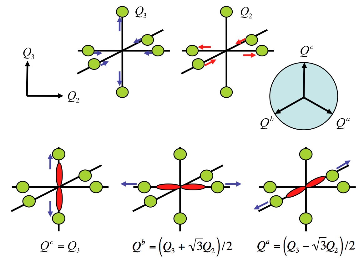
Figure 18: Jahn-Teller distortions of $e_{g}$ symmetry, $Q_{2}$ and $Q_{3}$, of a transition metal - oxygen octahedron. The orbital degree of freedom $(T_{i}^{z},T_{i}^{x})$ is locked to the distortion $(Q_{3},Q_{2})$

This model is that of the 120^∘ model of Eqs.(19, 23). Note that unlike the realization of Eq. (82), the 120^∘ model of Eq. (102) derived from Jahn-Teller distortions is essentially classical: the zero point quantum oscillations of the heavy oxygen ions that mediate the orbital-orbital interactions (or equivalently, the interactions between Jahn-Teller centers) are negligible.

V.1.7 Charge Transfer Effects Through Ligand Sites

So far, the electronic hopping have been implied to occur directly from a $d$-orbital on one site to a $d$-orbital on a neighboring site. In many oxides however such hoppings from $d$ to $d$ state occur via an oxygen $p$ orbital of an oxygen ion that is bridging two transition metal ions. This is particularly relevant for oxides that are charge transfer isolators Zaanen et al. (1985). In these materials the charge transfer through ligand sites is dominant when the energy for an electron transfer $\Delta$ between the ligand and the transition metal ion is smaller than the energy penalty $U$ for direct charge transfer between two transition metal ions.

However, it can be easily shown that the effective hoping integrals between $e_{g}$ and $t_{2g}$ states do not change their symmetry if hopping is occurring via an oxygen ligand bridging the two transition-metal sites and the emerging Kugel-Khomskii and compass models for the orbital and/or spin degrees of freedom in the strong coupling limit of large $U$, remain unaltered. This situation changes fundamentally when the TM-oxygen-TM bond is not 180 degrees, which is in particular the case for edge-sharing octahedra, where this bond is (close to) 90 degrees Mostovoy & Khomskii (2002).

The effective orbital-only and orbital-dependent spin exchange Hamiltonians that result when charge transfer though ligand sites is the dominant conduit for charge excitations between transition metal ions leads to compass type Hamiltonians which are different from which we discussed thus far Mostovoy & Khomskii (2004). Most notably, an orbital only Hamiltonian appears which does not result from Jahn-Teller distortions which may account for the far higher orbital ordering transition temperature as opposed to spin ordering in these materials. Unlike the KK model (in which spin and orbital degrees of freedom are correlated), the orbital only Hamiltonian which remains in the limit of $U\to\infty$ is asymmetric between hole and electron excitations. When pairs of transition metal ions with a single hole (h) on the doubly degenerate e_g orbitals [e.g., Cu²⁺ ions that have an outer-shell structure of $t^{6}_{2g}e^{3}_{2g}$] interact with one another through ligand sites (the ligand holes are assumed to be dispersion-less), Mostovoy & Khomskii (2004) in the limit $U\to\infty$ (leaving the charge transfer $\Delta$ as the only remaining finite energy scale), the effective resultant charge transfer orbital-only Hamiltonian assumes the form

$$H^{(h)}_{CT}=\frac{2t^{2}}{\Delta^{3}}\sum_{i,\gamma}(\frac{1}{2}+\pi^{\gamma}_{i})(\frac{1}{2}+\pi^{\gamma}_{i+{\bm{e}}_{\gamma}}).$$ (103)

In Eq. (103), $t$ is the hopping amplitude between the transition metal ion and the ligand site. The operators $\pi^{\gamma}$ are of the same form as in Eqs. (23,82). Similarly, for transition metal ions that have one electron (e) in the doubly degenerate $e_{g}$ states, the effective interaction that remains in the large $U$ limit is of the form

$$H^{(e)}_{CT}=\frac{2t^{2}}{\Delta^{3}}\sum_{i,\gamma}(\frac{3}{2}-\pi^{\gamma}_{i})(\frac{3}{2}-\pi^{\gamma}_{i+{\bm{e}}_{\gamma}}).$$ (104)

A single electron in the $e_{g}$ for which Eq. (104) my be relevant can be that of ions such as Mn³⁺ Cr²⁺ (both of which have an ($t_{2g}^{3}e_{g}^{1}$) structure) as well as the low spin Ni³⁺ ($t_{2g}^{6}e_{g}^{1}$) which we earlier encountered when reviewing NaNiO₂ Mostovoy & Khomskii (2002). The Hamiltonians of Eqs. (103,104) capture the effect of common ligand sites which are shared by the transition metal ions. For finite values of $U$, a compass type coupled spin and orbital Hamiltonian different from the Kugel-Khomskii Hamiltonian further appears. The fact that this spin and orbital Hamiltonian is of a smaller size, for large $U$, than the orbital only Hamiltonians of Eqs. (103, 104) may, as hinted at above, rationalize the higher values of the orbital ordering temperatures as compared to the spin ordering temperatures that are commonly observed. Similarly for finite $U$, there are additional corrections to the orbital only Hamiltonians of Eqs. (103, 104)). The energetics associated with these Hamiltonians favors orbital and spin states which differ from those that would be chosen by the Jahn-Teller or Kugel-Khomskii Hamiltonians alone. An additional marked feature of the orbital only interactions that result is, as is clearly seen in Eqs. (103, 104), the appearance of linear terms in the pseudospins. Such terms are not present in the Jahn-Teller Hamiltonian. These linear terms effectively act as external effective fields that couple to the pseudospins and may help account for empirically observed orbital structure which is not favored by Jahn-Teller nor Hubbard (and thus also Kugel-Khomskii) type Hamiltonians Mostovoy & Khomskii (2004).

V.1.8 Strong Relativistic Spin-Orbit Coupling

As noted in Section II.2, hybrid models interpolating between a Heisenberg model and compass models have been introduced in various physical contexts (van den Brink (2004), Chaloupka et al. (2010), Chern et al. (2010)). Such models are relevant to describe superexchange interactions in transition metal systems with large spin-orbit coupling, which appears 4d and 5d transition metal ions (see Fig. 10) such as Rh, Ru, Os, and Ir. This spin-orbit coupling mixes the orbital and spin degrees of freedom of an ion, into an effective moment that carries both orbital and spin character. In a Mott insulator the moments on different ions couple to each other via superexchange process.

In what follows, we will discuss the viable physical realization of the Heisenberg-Kitaev model. The properties and phase diagram of this type of Heisenberg-Kitaev model are reviewed in Sec. IX.12. We review a specific type first of these interactions as first introduced by Jackeli & Khaliullin (2009) in their study of Mott insulators and, specifically, several iridates. More recently, some other iridates (including the compounds A₂IrO₃ with A an alkaline metal such as Na or Li or a lanthanide that will focus on in this section) have witnessed a flurry of activity due to interest in their possible potential as topological insulators, e.g., Shitade et al. (2009); Yang, B-J. & Kim, Y-B. (2010); Wan et al. (2011); Balents (2011). Other notable families include iridates with a pyrochlore A₂Ir₂O₇ or a hyper-kagome structure A₄Ir₃O₈. Strong spin-orbit couplings were seen to lead to unique Mott insulating states Kim et al. (2008). The couplings between the spin and orbital degrees of freedom on such lattices can lead to compass type interactions. We first review the physical considerations underlying the specific “honeycomb iridates” that form the focus of present interest. In compounds of the A₂IrO₃ type, iridium (Ir⁴⁺) ions at the centers of IrO₆ octahedra form a layered honeycomb lattice (see Fig. 19).

Figure 19: The crystallographic structure of Na₂IrO₃. The Na, Ir, and O atoms are shown as blue (black), red (dark gray), and yellow (light gray) spheres, respectively. (a) The view perpendicular to the $c$ axis showing the layered structure with layers containing only Na atoms alternating slabs of NaIr₂O₆ stacked along the $c$ axis. The IrO₆ octahedra are shown in pink with the (red) Ir atoms sitting in the middle. (b) One of the NaIr₂O₆ slabs viewed down the c axis to highlight the honeycomb lattice of Ir atoms within the layer. The Na atoms occupy voids between the IrO₆ octahedra Singh & Gegenwart (2010).

Large spin-orbit coupling appears 4d and 5d transition metal ions such as Rh, Ru, Os, and Ir. The large mass of the iridium ion ($Z=77$) leads to a spin-orbit coupling constant as large as $\lambda\sim 380$ meV in Ir⁴⁺ ions Schirmer et al. (1984). Direct measurements of the insulating iridates Sr₂IrO₄ Kim et al. (2012b), Sr₃Ir₂O₇ Kim et al. (2012a), as well as Na₂IrO₃ directly attest to the spin-orbit couplings that they exhibit. Strong crystal field effects of octahedral oxygen cage split the 5d⁵ configuration of the typical Ir⁴⁺ valency and lead to the occupation of the five electrons (or single hole) in the three low energy t_2g states. The considerations below apply to magnetic Ir⁴⁺ and other (e.g., Rh⁴⁺) transition metal ions with a single hole in the t_2g triplet.

The hole in the t_2g orbitals has an effective orbital angular momentum $L=1$ Abragam & Bleaney (1970). Specifically, $|L_{z}=0\rangle\equiv|xy\rangle$ and $|L_{z}=\pm 1\rangle\equiv-\frac{1}{\sqrt{2}}(i|xz\rangle\pm|yz\rangle)$. The t_2g sector is further splintered as follows. The local, ionic low energy Hamiltonian for the single hole

$$H=\lambda{\bm{L}}\cdot{\bm{S}}+\Delta L_{z}^{2}$$ (105)

contains both spin-orbit effects and a tetragonal splitting $\Delta$, which might be finite or zero depending on the coordination of the ligand ions. For an octahedral IrO₆ oxygen cage that is elongated along the $c$ axis direction the tetragonal splitting $\Delta>0$.

Spin-orbit coupling splits up the six basis states $|L_{z},S_{z}\rangle$ spanning the azimuthal angular momentum ($L_{z}$) and spin component $S_{z}$ (up or down) of the hole, into doublet and quartet. The low energy sector of the Hamiltonian of Eq. (105) is spanned by the following two states for the hole Jackeli & Khaliullin (2009)

$$|\Uparrow\rangle = \sin(\theta/2)|L_{z}=0,\uparrow\rangle-\cos(\theta/2)|L_{z}=1,\downarrow\rangle\ \ \ \$$

$$|\Downarrow\rangle = \sin(\theta/2)|L_{z}=0,\downarrow\rangle-\cos(\theta/2)|L_{z}=-1,\downarrow\rangle\ \ \ \$$ (106)

with $\tan\theta=2\sqrt{2\lambda}/(\lambda-2\Delta)$. The two states in Eq. (106) enable the definition of a SU(2) pseudo-spin operator such that $|\Uparrow\rangle$ and $|\Downarrow\rangle$ correspond, respectively, to its up and down eigenstates ($|\tau_{z}=1/2\rangle=|\Uparrow\rangle$ and $|\tau_{z}=-1/2\rangle=|\Downarrow\rangle$). These two states in Eq. (106) are related to each other by time reversal (and thus form a Kramers doublet). As a consequence of spin-orbit effects, the hole lies within the sector formed by these two states.

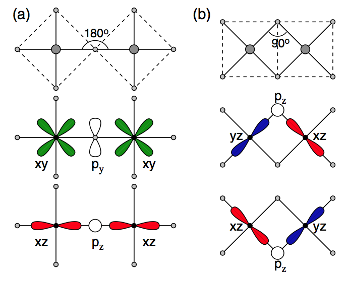
Figure 20: Two possible geometries of a TM-O-TM bond with corresponding orbitals active along these bonds. The large (small) dots stand for the transition metal (oxygen) ions. (a) A 180^∘-bond formed by corner-shared octahedra (see also Fig. 17), and (b) a 90^∘-bond formed by edge-shared octahedra.  Jackeli & Khaliullin (2009).

The Ir moments in Na₂IrO₃ become antiferromagnetically ordered at a Neel temperature $T_{N}\simeq 15K$ Liu et al. (2011)- a temperature which is notably lower than the paramagnetic Curie temperature (-125 K Singh et al. (2012)). Such a reduced ordering temperature is to be expected in frustrated systems and is natural within the Heisenberg-Kitaev” (HK) model  Jackeli & Khaliullin (2009); Chaloupka et al. (2010) which we will study in greater depth in Section IX.12. We now review the processes which may lead to precisely such a Hamiltonian in these systems.

Hopping through intermediate oxygen ligands:

Similar to our discussion in subsection V.1.7, we now consider the effect of intermediate ligand (i.e., oxygen) sites. In the case of cubic symmetry ($\Delta=0,\sin\theta=1/\sqrt{3}$), there are, generally, two dominant exchange paths for an exchange between two Ir ions at lattice sites $i$ and $j$ via an intermediate oxygen ion Jackeli & Khaliullin (2009), see Fig. 20:

(i) 180^∘ paths. These are schematically depicted in the lefthand panel of Fig. 20. In this case, the hopping is diagonal is the orbital index. For instance, both a bond along the $x$ direction, as seen in panel (a) of Fig. 20, an $|xy\rangle$ state on the left TM ion may be coupled to an $|xy\rangle$ state on the right TM ion. Similarly, along such a link parallel to the cubic lattice $x$ direction, an $|xz\rangle$ state may be coupled to another $|xz\rangle$ state. The same applies with trivial alterations for bonds parallel to the $y$ or $z$ axis cubic lattice directions. Within the two state subspace of Eq. (106), the effective exchange interaction between the effective spin-orbital moments is given by

$$H_{ij}={\cal J}_{1}{\bm{\tau}}_{i}\cdot{\bm{\tau}}_{j}+{\cal J}_{2}({\bm{\tau}}_{i}\cdot\bm{e}_{ij})({\bm{\tau}}_{j}\cdot\bm{e}_{ij}),$$ (107)

where the coupling constants $J_{1,2}$ are dependent on hopping amplitudes, the (Hubbard type) Coulomb repulsion $U$ between two $t_{2g}$ electrons on the same ion and Hund’s coupling $J_{H}$ Jackeli & Khaliullin (2009). As throughout in this review, in Eq. (107), $\bf{e}_{ij}$ denotes a unit vector along the direction from point $i$ to point $j$. In the pertinent limit of strong spin-orbit coupling, the interaction of Eq. (107) is dominated by the isotropic Heisenberg type interaction with the anisotropy set by Hund’s coupling. In Na₂IrO₄ and other iridates, the dominant exchange paths are not those of the 180^∘ type via an intermediate oxygen lying on the line between neighboring Ir ions. Rather, the dominant mechanisms via intermediate oxygen orbitals are those involving oxygen ions that lie at 90^∘ off relative to the line between the TM ions (see panel (b) of Fig. 20). We turn to these next.

(ii) 90^∘ bonds. In such geometries, several mechanisms are possible. In these, unlike the 180^∘ bonds reviewed above, the dominant couplings between the $d$ electron orbital states are non-diagonal in the orbital index: different orbital states are coupled to each other. We first comment on the case of (intra-orbital sector) coupling between two $t_{2g}$ (orthogonal) states and then discuss an important inter-orbital process that couples an $e_{g}$ orbital to a $t_{2g}$ state.

(a) There are two dominant intra-orbital $t_{2g}$ couplings:

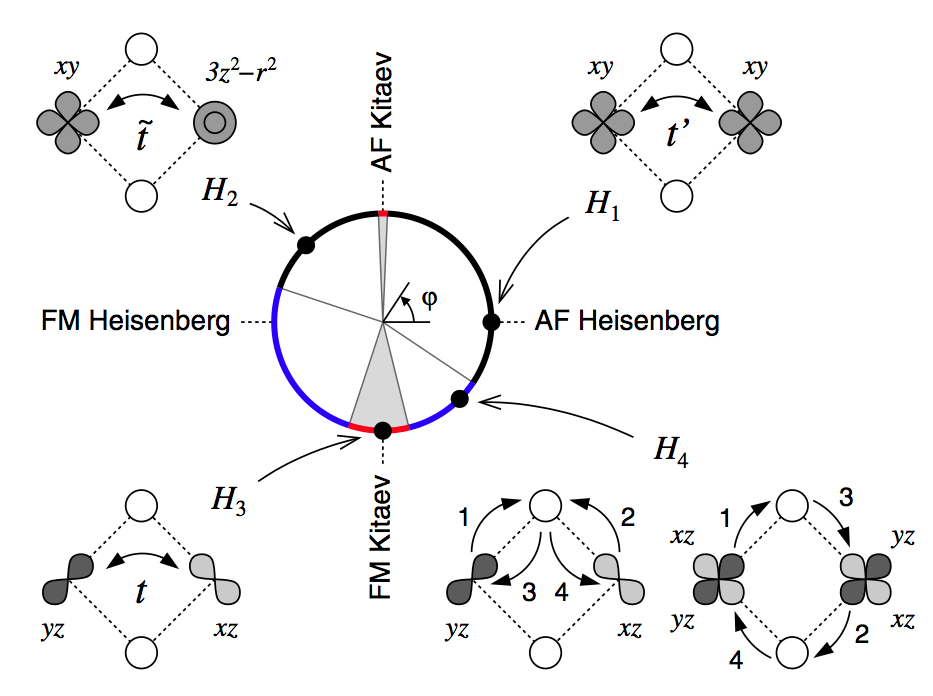
Figure 21: Schematics of four different exchange processes Chaloupka et al. (2013).

$\bullet$ $t_{2g}$-$t_{2g}$ coupling resulting from hopping between two TM ions via intermediate oxygen ions (See also process $H_{3}$ of Fig. 21.) as well as the righthand panel of Fig. 20). For links $(ij)$ with a TM-O-TM angle 90^∘, the superexchange between theTM ions along the cubic $\gamma$ axis, is mediated via two ligands that are perpendicular to that axis, the effective exchange reads

$$H^{superexchage}_{ij}=-{\cal J}^{ex}\tau_{i}^{\gamma}\tau_{j}^{\gamma}.$$ (108)

The exchange coupling ${\cal J}^{ex}\simeq\frac{8}{3}\frac{t^{2}J_{H}}{U^{2}}$ where $t$ is the indirect hopping amplitude between nearest neighboring $t_{2g}$ orbitals via intermediate oxygen ions.

$\bullet$ $t_{2g}$-$t_{2g}$ coupling via $pd$ charge transfer excitations (of energy $\Delta_{pd}$)

such as those schematically illustrated in (process $H_{4}$ of Fig. 21)
– In the first of such processes (that of the lefthand side of process $H_{4}$ of Fig. 21), two TM holes may hop to the same oxygen site wherein there is a Coulomb repulsion of strength $U_{p}$). The energy associated with such a process is

$$H^{transfer}_{ij}\simeq-\frac{8}{9(\Delta_{pd}+\frac{U_{p}}{2})}\tau_{i}^{\gamma}\tau_{j}^{\gamma}.$$ (109)

– In a second process, two holes may go (either clockwise or counter-clockwise within a loop) through the sites of a plaquette (as in the righthand process of $H_{4}$ of Fig. 21). This leads to a contribution

$$H^{plaquette}\simeq\frac{8}{9\Delta_{pd}}\tau_{i}^{\gamma}\tau_{j}^{\gamma}.$$ (110)

(b) Inter-orbital $t_{2g}$- $e_{g}$ hopping $\tilde{t}$ via an intermediate oxygen (as in the process of $H_{2}$ of Fig. 21). This is the dominant Chaloupka et al. (2013) mechanism in a 90^∘ bonding geometry. In the iridates, this contribution is borne by the sizable $t_{pd\sigma}$ overlap between the oxygen $2p$ and $e_{g}$ orbital of the TM ion. Along a cubic lattice direction $\gamma$, Khaliullin (2005a)

$$H^{inter-orbital}_{ij}={\cal{J}}^{i-o}[2\tau_{i}^{\gamma}\tau_{j}^{\gamma}-{\bm{\tau}}_{i}\cdot{\bm{\tau}}_{j}].$$ (111)

Within the Mott-insulating iridates, ${\cal{J}}^{i-o}\simeq\frac{4}{9}({\tilde{t}}/{\tilde{U}})^{2}{\tilde{J}}_{H}$ where Chaloupka et al. (2013) $\tilde{J}_{H}$ is Hund’s coupling between $t_{2g}$ and $e_{g}$ orbitals and $\tilde{U}$ is the Coulomb penalty associated with $t_{2g}$-$e_{g}$ hopping. Typically, in the iridates, ${\tilde{t}}/t/t\sim 2$ rendering these interactions very notable. The origin of the form of ${\cal{J}}^{i-o}$ is transparent as we briefly review. The factor of $(\tilde{t}/\tilde{U})^{2}$ provides the probability that a $t_{2g}$ spin is transferred to a nearest neighbor $e_{g}$ orbital; on arrival at that orbital of the nearest neighbor ion, the transferred spin has to obey Hund’s rule with the “host” $t_{2g}$ spin Khaliullin (2005a); Chaloupka et al. (2013).

Direct hopping between $t_{2g}$ orbitals:

Supplanting all of these exchange paths above through an intermediate oxygen (whether of the 90^circ or 180^∘ type), there are also direct exchange interactions (as in the process $H_{1}$ of Fig. 21). These lead to a Heisenberg type standard spin exchange result

$$H^{direct}=\frac{4}{9}\frac{(t^{\prime})^{2}}{U}[{\bm{\tau}}_{i}\cdot{\bm{\tau}}_{j}],$$ (112)

where $t^{\prime}$ denotes the direct hopping amplitude between the $t_{2g}$ electrons.

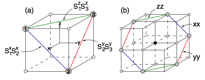
Figure 22: Examples of the structural units formed by $90^{\circ}$ TM-O-TM bonds and corresponding spin-coupling patterns. Gray circles stand for magnetic ions, and small open circles denote oxygen sites. (a) Triangular unit cell of ABO₂-type layered compounds, periodic sequence of this unit forms a triangular lattice of magnetic ions. The model on this structure is a realization of a quantum compass model on a triangular lattice: e.g., on a bond $1-2$, laying perpendicular to x-axis, the interaction is $\tau^{x}_{1}\tau^{x}_{2}$. (b) Hexagonal unit cell of A₂BO₃-type layered compound, in which magnetic ions (B-sites) form a honeycomb lattice. (Black dot: nonmagnetic A-site). On an $xx$-bond, the interaction is $\tau^{x}_{i}\tau^{x}_{j}$, etc. For this structure, the model (3) is identical to the Kitaev model Jackeli & Khaliullin (2009).

In an ABO₂ system with A (and B) being non-magnetic alkali (TM magnetic) ions, a layered triangular geometry with 90^∘ type exchange processes between the magnetic B ions appear. [See also our earlier discussion of NaNiO₂ in subsection V.1.3.] Further dilution of this system, as in A₂BO₃ systems leads to a layered honeycomb type structure of the magnetic B ions, see Fig. 22. On such a geometry, the 90^∘ processes lead to Kitaev type interactions augmenting rotationally symmetric Heisenberg type exchange processes. These considerations apply to layered honeycomb iridates (B = Ir and A = Na or Li).

Putting all of the pieces together, exchange processes lead to an effective Hamiltonian in the projected subspace of Eq.(106) that is of the Heisenberg-compass form of Section II.2. In A₂BO₃ systems this compass model is of the Kitaev type. This Heisenberg-Kitaev (HK) model, in the form that it is typically studied Chaloupka et al. (2010), is

$$H_{HK} = -J_{1}\sum_{\langle ij\rangle_{\gamma}}\tau_{i}^{\gamma}\tau_{j}^{\gamma}+J_{2}\sum_{\langle ij\rangle}{\bm{\tau}}_{i}\cdot{\bm{\tau}}_{j}\ \ \ \$$ (113)

$$\equiv C\Big{[}-2\alpha\sum_{\langle ij\rangle_{\gamma}}\tau_{i}^{\gamma}\tau_{j}^{\gamma}+(1-\alpha)\sum_{\langle ij\rangle}{\bm{\tau}}_{i}\cdot{\bm{\tau}}_{j}\Big{]}\ \ \ \$$

$$\equiv A\Big{[}2\sin\varphi\sum_{\langle ij\rangle_{\gamma}}\tau_{i}^{\gamma}\tau_{j}^{\gamma}+\cos\varphi\sum_{\langle ij\rangle}{\bm{\tau}}_{i}\cdot{\bm{\tau}}_{j}\Big{]}.$$

Eq. (113) constitutes a particular realization of Eq. (38). The parameterizations of the coupling constants $J_{1}$ and $J_{2}$ in terms of $(C,\alpha)$ or $(A,\varphi)$ are prevalent in the literature and are natural in disparate contexts. We will return to these in subsection IX.12. In early works within the field, the focus has been on systems with ferromagnetic $(J_{1}>0$) Kitaev couplings. It was later realized Chaloupka et al. (2013) that antiferromagnetic Kitaev type interactions can be notable due to the process of Eq. (111); these contributions lead, consistent various experimental measurements, to zig-zag type magnetic ordering Singh & Gegenwart (2010); Liu et al. (2011); Singh et al. (2012); Choi et al. (2012).

Effective related models with longer ranger interactions were advanced by Kargarian et al., 2012, introducing a Hubbard model with next nearest neighbor hopping on a honeycomb lattice – the pertinent geometry of the layers. The Hamiltonian is given by

$$H= -t\sum_{\langle ij\rangle,\alpha}c_{i\alpha}^{\dagger}c_{j\alpha}+\sum_{\langle\langle ij\rangle\rangle_{\alpha}}\sum_{\alpha\beta}t_{\alpha\beta}^{\gamma}c_{i\alpha}^{\dagger}c_{j\beta}$$ (114)

$$+U\sum_{i}n_{i\uparrow}n_{i\downarrow}.$$

In Eq. (114), $\alpha,\beta=\uparrow,\downarrow$ denote spin-orbital coupled pseudo-spin states, $U$ is the standard Hubbard Coulomb penalty term, $t$ is the hopping amplitude between nearest neighbor sites on the lattice, and the compass-type next nearest neighbor hopping $t^{\gamma}=-t^{\prime}+it^{\prime\prime}\sigma^{\gamma}$ where $\sigma^{\gamma}$ are Pauli operators; the flavors $\gamma=x,y,$ or $z$ of the Pauli operators are given by the relative orientation of the next nearest sites $i$ and $j$. On the honeycomb lattice, the vector connecting next neighbor sites can be along one of three directions. In the strong coupling limit, $U\gg t$, Eq. (114) reduces to a longer range counterpart of the Heisenberg- Kitaev models discussed in section II.2. See Eq. (38) in particular. This is given by Kargarian et al. (2012)

$$H = J_{1}\sum_{\langle ij\rangle}{\bf{\tau}}_{i}\cdot{\bf{\tau}}_{j}-J_{2}\sum_{\langle\langle ij\rangle\rangle}{\bf{\tau}}_{i}\cdot{\bf{\tau}}_{j}$$ (115)

$$+J_{3}\sum_{\langle\langle ij\rangle\rangle}\tau_{i}^{\gamma}\tau_{j}^{\gamma}.$$

where $J_{1}=4t^{2}/U,J_{2}=4[(t^{\prime})^{2}-(t^{\prime\prime})^{2}]/U$ and $J_{3}=8(t^{\prime\prime})^{2}/U$.

V.2 Vacancy Centers and Trapped Ions

As noted earlier, the Heisenberg-Kitaev model of Eq. (113) represents a specific type of the compass-Heisenberg models discussed in Section II.2. Hamiltonians of the form of Eq. (38) may also describe vacancy center systems Trousselet et al. (2012).Such systems are afforded by, e.g., arrays of nitrogen vacancy (NV) centers in diamond Gaebel et al. (2006); Neumann et al. (2010). When hyperfine and other effects may be neglected, vacancy arrays may, in some instances, be modeled by quantum pseudo-spins that are predominantly coupled via effective dipolar interactions that contain both a couplings of the Heisenberg exchange variety along with compass type interactions,

$$H_{dipolar}=\sum_{\langle ij\rangle_{\gamma}}\frac{A}{r_{ij}^{3}}({\bf{T}}_{i}\cdot{\bf{T}}_{j}-3T_{i}^{\gamma}T_{j}^{\gamma}),$$ (116)

where the pseudo-spin ${\bf T}_{i}$ now represents the dipole moment at lattice site $i$ and $A$ is a system dependent constant. In such lattices formed by vacancies, the dipole interactions have a compass type, anisotropic, component (the second term in Eq. (116)) which depends on the projection of the effective dipoles along the external lattice directions $\gamma$ (the latter directions are defined by the directions of lattice vectors linking interacting nearest neighbor lattice sites). The sum of the two (anisotropic and isotropic) terms in Eq. (116), capturing interactions between these effective dipoles on the lattice, leads to a compass-Heisenberg type system Trousselet et al. (2012). Dipole type interactions also arise in trapped ion systems Schmied et al. (2011). Already on the classical level, the direction dependence of the dipolar interactions leads to notable differences in thermodynamic properties and correlations Chakrabarty & Nussinov (2011) from dipolar interactions that include the isotropic component alone.

V.3 Cold Atom Systems

In recent years, the ability to manipulate cold atom (and molecule) systems in standing wave laser beams has enabled the generation of systems with tunable interactions. In essence, laser beams enable to generate confining potentials and a crystal of light in which the lattice sites serve as energy minima for the location of dilute atoms or molecules.

Gaining understanding of electronic and magnetic effects is in a solid typically complicated by, for example, the presence of impurities, and the long-range nature of Coulomb interactions and in general the rather limited possibility to change parameters and interactions. Ultracold atoms in optical lattices provide a great advantage in allowing to probe model Hamiltonians that capture the essential many-body physics of strongly correlated electron systems in a controllable and clean experimental setting D. Jaksch (2005); Bloch et al. (2008). Relevant parameters can be independently controlled, thus allowing quantitative comparisons of the experiment and theory.

In particular the Hubbard Hamiltonian for both bosonic Jaksch et al. (1998); Greiner et al. (2002); Stöferle et al. (2004) and fermionic particles Schneider et al. (2008) on optical lattices has been realized, also in the Mott insulating regime. This has opened the road to prepare other effective spinor models with ultracold atoms on the lattice, such as the ones of compass and Kitaev type, which we review in this section.

Proposals for the creation of compass-type models in the ultra-cold gas setting can be classified into three categories. The first one is to use an ensemble of ultra-cold bosonic or fermionic atoms with two relevant internal states and engineer the hopping amplitudes by additional laser fields Duan et al. (2003). The second category is to use atoms that are in $p$-like states, the orbital degeneracy of which constitutes the pseudo-spin degree of freedom, which can be created either by excitation out of $s$-like states or by filling a site with more than one fermionic atom Isacsson & Girvin (2005); Köhl et al. (2005); Browaeys et al. (2005); Müller et al. (2007); Anderlini et al. (2007); Kuklov (2006); Liu & Wu (2006); Wu et al. (2006); Wu (2008); Wu & Zhai (2008); Wu & Das Sarma (2008); Zhao & Liu (2008). Finally, by manipulating ultra cold dipolar molecules anisotropic spin interactions can be generated Micheli et al. (2006); Weimer .

V.3.1 Engineering Tunneling Amplitudes

In an ensemble of ultra-cold bosonic or fermionic atoms with two relevant internal states, a T=1/2 pseudospin, confined in an optical lattice, the pseudospin dependent tunneling between neighboring atoms in the lattice can be controlled. As reviewed in Sec. V.1.3, full control of these hopping amplitudes is in the Mott insulating regime of the Hubbard model enough to construct any compass-type Hamiltonian. In both Bose and Fermi systems, the anisotropy of the exchange in particular tunneling directions can be engineered by applying blue-detuned standing-wave laser beams along those directions  Duan et al. (2003); Kuklov & Svistunov (2003).

V.3.2 Bosonic Gases with Orbital Degree of Freedom

In the ground state, the atoms in an optical lattice are centered about their local minima provided by the confining potential of the laser beams which in the vicinity of its minima is harmonic. The atomic states in the lowest Bloch band are, essentially, the ground of the harmonic oscillator (more precisely, the product of single harmonic oscillator centered about each of the minima of the periodic confining potential generated by the laser beams) and those within the first excited Bloch band correspond to the first excited states of a harmonic oscillator.

Several approaches are available for transferring cold atoms to the first excited $p$-orbital band, for instance by applying an appropriate vibrational pulse with frequency on resonance with the $s$-$p$ state transition Liu & Wu (2006). A theory for the interactions in a dilute system of bosons in which the two lowest Bloch bands of a three dimensional optical lattice are considered was developed by Isacsson & Girvin (2005).

The central point in all of this is that in the cold atomic gas there are three such excited state corresponding to an ”excitation” along each of the three Cartesian directions (which for a single atom about its local confining potential minimum, which for symmetric confining potentials along all three directions, are of the form $xe^{-(r/a)^{2}}$, $ye^{-(r/a)^{2}}$ and $ze^{-(r/a)^{2}}$, with $r^{2}=x^{2}+y^{2}+z^{2}$ and $a$ the harmonic confining potential length scale. Henceforth these excitations are labelled as $p=X$, $Y$, $Z$.

The $p$-states are rather confined along all Cartesian directions apart from one and in that sense resemble atomic $p$-orbital. In the presence of Hubbard-type local interactions between the bosons the resulting system is thus of a compass type, where the pseudo-spins emerge from bosonic degrees of freedom. The strength of the confining potential along the three Cartesian directions can be tuned by the optical lattice. In the symmetric case, the resulting effective Hubbard type model taking into account on-site interactions of strength $U$ between the atoms is the form Isacsson & Girvin (2005)

$$H_{IG} = \sum_{i,p}\Big{(}E_{i}(i)n_{i}^{(p)}+\frac{U_{pp}}{2}n_{i}^{p}(n_{i}^{p}-1)\Big{)}$$ (117)

$$+ \sum_{i,p\neq p^{\prime}}U_{pp^{\prime}}\Big{(}n_{i}^{p}n_{i}^{p^{\prime}}+\frac{1}{2}(p_{i}^{\dagger}p_{i}^{\dagger}p_{i}^{\prime}p_{i}^{\prime}+h.c.)\Big{)}$$

$$- t\sum_{\langle i,i^{\prime}\rangle_{p},p}(p_{i}^{\dagger}p_{i^{\prime}}+h.c.).$$

The operators $p_{i}^{\dagger}$ and $p_{i}$ correspond to the creation and annihilation operators for an excited boson of flavor $p=X,Y,Z$ at site $i$. The constants $U_{pp^{\prime}}$, $U_{pp}$, and $E_{i}$ are determined by the parameters describing the confining optical potential. In a similar vein, if the confining potential along, say, the $z$ direction is much larger than along the $x$ and $y$ directions, the system is effectively two dimensional ($p=X,Y$ in Eq. 117 above). Physically, the Hamiltonian then describes two boson species (of type $X$ and $Y$) each of which may propagate only along one direction. The interaction terms enable two bosons of type $X$ to fuse and generate two bosons of type $Y$ (and vice versa).

There is a formal connection between a system of hard core bosons where the on-site repulsion $U\to\infty$ and no two bosons can occupy the same site and the pseudo-spin variants of the compass models. Towards this end, one can employ the Matsuda-Matsuda transformation Matsubara & Matsuda (956) relating a two flavor system of hard core bosons (e.g., bosons of type $X$ and $Y$) and the two states of a pseudo-spin $T=1/2$ particle.

V.3.3 Fermionic Gases with Orbital Degree of Freedom

Fermionic realizations of compass type systems have also been considered in optical lattices Wu (2008); Zhao & Liu (2008). A situation with a strong confining potential along e.g. the spatial $z$ direction will again lead to a two dimensional system. Wu (2008) focused on atomic orbitals and considered a situation in which there are two fermions per site with one of the fermions in an inert $s$ shell and the other occupying the $p$ bands (which in the case of strong optical confinement along the vertical ($z$) direction is restricted to the one of the two $p-$states (i.e., $p_{x}$ and $p_{y}$ orbitals). Hopping within the $p$ band states can be of either of the $\sigma$ bonding ($t_{||}$)- wherein there is a head on overlap of one electronic lobe of one site with another (parallel) single electronic $p$ lobe on a neighbor site- the wave-functions are parallel to the spatial direction linking the two sites or of the $\pi$ bonding ($t_{\perp}$) type where the $p$ wave-functions on two neighboring sites are orthogonal to the axis that links these two sites. Due to the far smaller overlaps involved in $\pi$ bonding, the $\sigma$ bonding is typically far stronger ($t_{||}/t_{\perp}\gg 1$). In what follows $\pi$ effects will be neglected. The directional character of the $\sigma$ bonding underlies the compass type interactions in this system. Orbitals in the $p_{x}$ state have a high tunneling amplitude only the $x$ direction and similarly orbitals in the $p_{y}$ state have a high tunneling and lead to consequent effective interactions only along the $y$ direction. Scattering in the $p$ wave channel as well as enhancements by magnetic effects and proximity to the Feshbach resonance can lead to a substantial Hubbard like interaction

$$H_{Hubbard}=U\sum_{i}n_{i,x}n_{i,y}.$$ (118)

In Eq. 118, with $p_{i,x}^{\dagger}$ and $p_{i,x}$ denoting the creation and annihilation operators for an electron in the $p_{x}$ orbital at site $i$, the operators $n_{i,x}=p_{i,x}^{\dagger}p_{i,x}$ and $n_{i,y}=p_{i,y}^{\dagger}p_{i,y}$ are the number operators for states of the $p_{x}$ and $p_{y}$ type respectively on the lattice site $i$. We may define $T=1/2$ pseudo-spin operators to be Wu (2008); Zhao & Liu (2008)

$$\tau_{1} = \frac{1}{2}(n_{x}-n_{y}),$$

$$\tau_{2} = \frac{1}{2}(p_{x}^{\dagger}p_{y}+H.c.),$$

$$\tau_{3} = -\frac{i}{2}(p_{x}^{\dagger}p_{y}-H.c.).$$ (119)

The $p_{x,y}$ states are eigenstates of $\tau_{1}$ with eigenvalues $\pm 1/2$ respectively. The compass type character emerges naturally. The $\sigma$-bonding exchange between two sites separated along, say, the Cartesian $x$ lattice direction. In that case, for large $U$ where a perturbative expansion in $t_{||}/U$ about the degenerate ground state of Eq. 118 (that of a single $p_{x}$ or $p_{y}$state per site) is possible. Second order perturbation theory in the kinetic $t_{||}$ term gives rise to an effective Ising type exchange $H_{ex}=J_{||}\tau_{i,1}\tau_{i+{\bf{e}}_{x},1}$ with $J_{II}=2t_{||}^{2}/U$ Wu (2008); Zhao & Liu (2008). Let us now consider the case of general quantization axis and separation between neighboring sites on the lattice. Similar to compass models in other arenas (in particular in orbital physics of the transition metal oxides), a simple but important feature of the underlying quintessential physics is that the Ising quantization axis will change with different orientations of the link connecting neighboring lattice sites. For a lattice link of general direction ${\bf{e}}_{\theta}=\cos\theta{\bf{e}}_{x}+\sin\theta{\bf{e}}_{y}$, it is possible to rotate the $p_{x,y}$ orbitals by $\theta$ to restore the situation above. This change of basis effects $p_{x}^{\prime}=p_{x}\cos\theta+p_{y}\sin\theta$ and $p_{y}^{\prime}=p_{y}\cos\theta-p_{x}\sin\theta$. These two states $p_{x,y}^{\prime}$ are eigenstates of the operator $\tau_{1}^{\prime}=(\tau_{1}\cos 2\theta+\tau_{2}\sin 2\theta)$. The exchange interaction for general orientation of a link between nearest neighbor sites is thus Wu (2008); Zhao & Liu (2008)

$$H_{ex}(i,i+{\bf{e}}_{\theta})=J_{||}[{\bm{\tau}}_{i}\cdot{\bf{e}}_{2\theta}][{\bm{\tau}}_{i+{\bf{e}}_{\theta}}\cdot{\bf{e}}_{2\theta}].$$ (120)

As in other orbital systems, once the interaction along one link (Eq. 120) in known, the Hamiltonian for the entire lattice can be pieced together by summing over all links in the lattice (taking into account their different spatial orientation ${\bf{e}}_{\theta}$).

V.3.4 Fermions in an Optical Lattice

In three dimensions, similar considerations recently led to the introduction of the Gell-mann compass models of Chern and Wu Chern & Wu (2011) on the cubic and diamond (Eqs. (122,123)) and more general lattices as we now review. As in the two-dimensional case, each site of the lattice hosts two fermions with one electron filling the inert $s$-orbital. In three-dimensions, the remaining electron can be in any one of the three $p-$ orbitals ($p_{x},p_{y}$ or $p_{z}$). Replicating the arguments presented above for two-dimensions Chern & Wu (2011), in the limit $U\gg t_{||}\gg t_{\perp}$, Chern and Wu arrived at the following Hamiltonian Chern & Wu (2011)

$$H_{CW}=-J\sum_{\langle ij\rangle}[P_{i}^{{\bm{e}}_{ij}}(1-P_{j}^{{\bm{e}}_{ij}})+[(1-P_{i}^{{\bm{e}}_{ij}})P_{j}^{{\bm{e}}_{ij}}].$$ (121)

In Eq. (121), ${\bm{e}}_{ij}=(e_{ij}^{x},e_{ij}^{y},e_{ij}^{z})$ is the bond direction (along which $t_{||}$ dominates for the orbital $|{\bm{e}}_{ij}\rangle=e_{ij}^{x}|p_{x}\rangle+e_{ij}^{y}|p_{y}\rangle+e_{ij}^{z}|p_{z}\rangle$ (over the transverse hopping $t_{\perp}$)). The projection operator $P^{{\bm{e}}_{ij}}=|{\bm{e}}_{ij}\rangle\langle{\bm{e}}_{ij}|$. The Hamiltonian of Eq. (121) embodies the ability of an electron in state $|{\bm{e}}_{ij}\rangle$ on site $i$ to hop in a direction parallel to ${\bm{e}}_{ij}$ to site $j$ if that site is unoccupied in that state (and vice versa). As in the standard Hubbard model, and the two-dimensional Hubbard type model discussed above, this kinetic hopping leads, for large $U$, to an effective exchange Hamiltonian in the presence of one relevant electronic degree of freedom per site.

When applied to the cubic and diamond lattice, this Hamiltonian reduces to the form provided in Eqs. (122, 123) Chern & Wu (2011).

Expressing, in the case of the cubic lattice model, the projection operators along the three crystalline directions ($\gamma=x,y,z$) as $P^{\gamma}=\frac{1}{3}(1+2{\bm{\lambda}}\cdot{\bm{e}}_{\gamma}$ and inserting this form into Eq. (121) leads, up an innocuous additive constant, to Eq. (122). Similarly, in the case of the diamond lattice, the projection operators may be written as $P=\frac{1}{3}(1+\sqrt{3}{\bm{\lambda}}\cdot{\bm{n}}_{\gamma})$ which reduces Eq. (121) to Eq. (123).

V.3.5 Spin interactions on a lattice

Ref. Micheli et al. (2006) discussed how to design general lattice spin systems by cold systems of polar molecules.

In cold gases of polar molecules, the spin degree of freedom originates the spin of an electron outside a closed shell of a hetero-nuclear molecule in its rotational ground state. The complete energy of the system is given by the sum of the translational kinetic and potential energies representing the confining potential of the laser system and two contributions which are of paramount importance in this setup- the individual rotational excitation energies of each molecule (that contains the nuclear angular momentum energy $B{\bf N}^{2}$ (with ${\bf N}$ the nuclear orbital angular momentum) and spin-rotation coupling (${\bf S}\cdot{\bf N}$)), and the dipole-dipole interactions between two molecules with the dipoles induced by the (nuclear) orbital angular momentum of each molecule. A key point is that large dipole-dipole interactions may be induced by a microwave field with frequency is near resonance with the transition $N=0\to N=1$ transition. An effective second order Hamiltonian in the ground state basis was obtained Micheli et al. (2006) which when averaged over the inter-molecular relative distance between members of a pair of molecules leads to an effective spin only interaction. The final effective Hamiltonian enables rather general interactions. The effective spin interactions are borne by the dipolar interactions induced by the microwave field. The interactions depend on the orientation of inter-molecular separations relative to the microwave field direction. In this setup spin orientation dependent compass type interactions appear very naturally.

V.3.6 Three-Flavor Compass Models

Even though the current focus on compass type interactions within various pseudospin systems, such interactions can arise in many other systems. One of their most natural incarnations is within bosonic and fermionic type systems. Of these the multi-orbital Hubbard model, from which the Kugel-Khomskii models are derived, is the simplest example Kugel & Khomskii (1982). As discussed in Section V.3.2, also in bosonic systems Isacsson & Girvin (2005), there may be two different types of particle species each of which may propagate along only one spatial direction. These particle species may interact with one another via on-site terms wherein two particles ”collide” along one axis and then convert into two particles that may propagate along an orthogonal direction.

One can also similarly define models in which there are several fermionic species- each of which have “compass type” hopping amplitudes and may, e.g., propagate only along one direction or more generally have anisotropic hopping amplitudes that differ from one species to another. Different types of such systems have been investigated Chern & Wu (2011) Here the concept is illustrated by specifically considering the incarnation of such system recently introduced by Chern and Wu Chern & Wu (2011). It leads to compass type systems referred to as Gell-mann matrix compass models. Unlike the $SU(2)$ isospins that formed the focus of our discussion thus far, the basic degree of freedom in these systems are Gell-mann operators.

Specifically, on the cubic lattice, these take the form Chern & Wu (2011)

$$H^{Gell-mann}_{3\Box}=\frac{8J}{9}\sum_{a=x,y,z}\sum_{\langle ij\rangle||\gamma}({\bm{\lambda}}_{i}\cdot{\bm{e}}_{\gamma})({\bm{\lambda}}_{j}\cdot{\bm{e}}_{\gamma}).$$ (122)

In Eq. (122), ${\bm{\lambda}}=\frac{\sqrt{3}}{2}(\lambda^{(3)},\lambda^{(8)})$ where the standard Gell-mann matrices $\lambda^{(3)}$ and $\lambda^{(8)}$ are diagonal and given by $\lambda^{(3)}=$diag$(1,-1,0)$ and $\lambda^{(8)}=$ diag$(1,1,-2)/\sqrt{3}$. As in the earlier compass model that we introduced thus far, $\gamma$ denotes the direction of the link between the nearest neighbor sites $i$ and $j$. Similar to the 120^∘ model, the three unit vectors in Eq. (122) are equidistant on a disk, ${\bm{e}}_{x,y}=(\pm\sqrt{3},1)/2$ and ${\bm{e}}_{z}=(0,-1)$.

On the diamond lattice Chern & Wu (2011),

$$H^{Gell-mann}_{3\diamond}=\frac{2J}{3}\sum_{\gamma=0}^{3}\sum_{\langle ij\rangle||\gamma}({\bm{\lambda}}_{i}\cdot{\bm{n}}_{\gamma})({\bm{\lambda}}_{j}\cdot{\bm{n}}_{\gamma}).$$ (123)

In this case, in Eq. (123), the vector ${\vec{\lambda}}=(\lambda^{(6)},\lambda^{(4)},\lambda^{(1)})$. The Gell-mann matrices $\lambda^{(1)},\lambda^{(4)}$, and $\lambda^{(6)}$ are non-diagonal (and do not commute amongst themselves). The index $\gamma=0,1,2,3$ denotes the four nearest neighbor directions on the diamond lattice with correspondingly $\{{\bm{n}}_{\gamma}\}$ denoting the unit vectors from a given lattice site to its nearest neighbors. (Specifically, when expressed in the Cartesian coordinate system, ${\bm{n}}_{0}=({\bm{e}}_{x}+{\bm{e}}_{y}+{\bm{e}}_{z})/\sqrt{3},{\bm{n}}_{1}=({\bm{e}}_{x}-{\bm{e}}_{y}-{\bm{e}}_{z})/\sqrt{3},{\bm{n}}_{2}=(-{\bm{e}}_{x}+{\bm{e}}_{y}-{\bm{e}}_{z})/\sqrt{3}$, and ${\bm{n}}_{3}=(-{\bm{e}}_{x}-{\bm{e}}_{y}+{\bm{e}}_{z}))/\sqrt{3}$. The motivation and properties of these models are reviewed in Sections V.3.4, IX.10.

V.4 Chiral Degrees of Freedom in Frustrated Magnets

Compass models also appear in effective low energy description of quantum magnets that have a chiral degree of freedom Budnik & Auerbach (2004); Capponi et al. (2004); Ferrero et al. (2003); Mila et al. (2007). In these systems, the chirality plays the role of the pseudo-spin with non-trivial directional dependence of the coupling. Similar to the pseudo-spin in orbital systems that enables us to track the different degenerate orbital states (belonging, e.g., to the different degenerate orbital sectors ($e_{g}$ and $t_{2g}$ in transition metal ions), in frustrated magnets with a basic building block (e.g., triangle or other) that leads to a multitude of ground states, the chirality tracks the extra degeneracy of ground states. In the quantum magnets that we will detail below, there are within each building block several degenerate ground states that are labeled by different values of the chirality. This degeneracy is lifted by interactions between the different building blocks (e.g., interactions between different triangular units in a kagome lattice) that rise to effective interactions involving chiralities on different basic units (triangles) which are precisely of the compass type. To date, two variants of the kagome lattice antiferromagnet were investigated in their low energy sector. These are the trimerized kagome lattice antiferromagnet Ferrero et al. (2003) and the uniform kagome antiferromagnet Budnik & Auerbach (2004). Both of these systems were investigated for a spin $S=1/2$ rendition of the original antiferromagnet. One way to describe the kagome lattice- which was made use of for both the trimerized and uniform systems- is, indeed, as a triangular lattice of triangles, see Fig. 23.

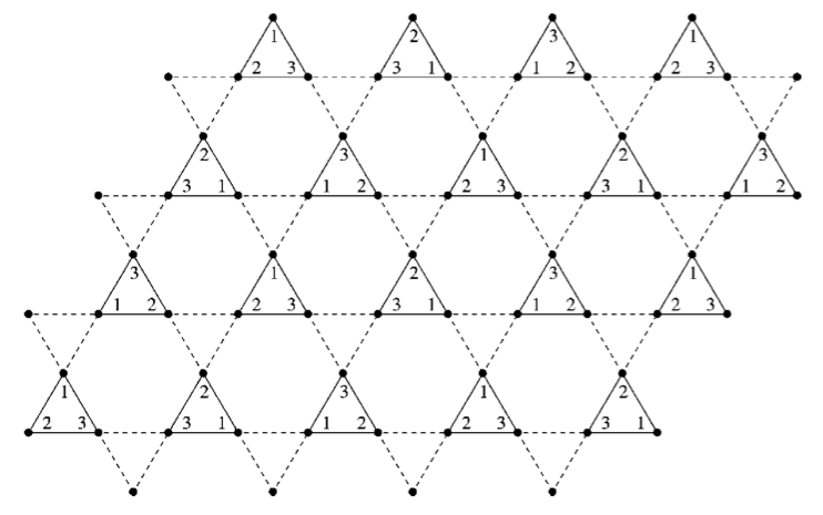
Figure 23: The trimerized kagome lattice. The solid and dashed lines indicate the antiferromagnetic coupling $J$ and $J^{\prime}$, respectively. The numbers 1, 2, and 3 indicate the site indexing inside the elementary triangles which defines the gauge. From Ferrero et al. (2003).

The kagome lattice has a very low coordination number. This along with the frustrated nature of the antiferromagnetic interactions around individual triangular loops lead the system to have a richness of low energy states and an extremely high degeneracy of classical ground states.

Below we will elaborate on the effective low energy description and consequent origin of the compass type interactions in both systems.

V.4.1 Non-uniform Trimerized Kagome Lattice Antiferromagnet

In systems such as the spin $S=3/2$ antiferromagnet SrCr_8-xGa_4+xO₁₉, the existence of triangular layers between the kagome lattice planes generates two types of effective bond strengths inside the kagome lattice plane. The resulting effective planar system- the trimerized kagome lattice antiferromagnet- highlights the geometry of the kagome lattice as a triangular lattice of triangles. Focusing on the upwards facing triangles, we see that they form a triangular lattice. Ferrero et al. (2003); Capponi et al. (2004) considered a spin $S=1/2$ model in which the nearest neighbor couplings inside the triangles ($J$) were far larger than the nearest neighbor couplings between sites on different’ triangles ($J^{\prime}$). In the limit $J^{\prime}/J\ll 1$, the trimerized kagome lattice antiferromagnet becomes a set of decoupled triangular units (with an antiferromagnetic exchange constant of $J$ within each triangular unit). The idea is then to employ perturbation theory in $J^{\prime}/J$ about this limit of decoupled antiferromagnetic triangular units.

Now, the problem of three spin $S=1/2$ on an antiferromagnetic ring (i.e., a basic triangular unit of the kagome lattice) spans $2^{3}=8$ states. In the total spin basis it can be decomposed into a Hilbert space sector that has a total spin $S_{tot}=3/2$ (spanning four states) as well as two sectors with total spin $S_{tot}=1/2$ (with each of these latter sectors, of course, spanning two states). Formally, that is, the direct product basis can decomposed in the total spin basis as $1/2\otimes 1/2\otimes 1/2=3/2\oplus 1/2\oplus 1/2$. In the antiferromagnetic problem, the tendency is to minimize the spin as much as possible. Indeed an immediate calculation that we will perform now shows that at low energies we can confine our attention to the four lower lying $S_{tot}=1/2$ ground states. Towards that end, we very explicitly note that for a three-site antiferromagnetic problem on a triangle,

$$J({\bf S}_{1}\cdot{\bf S}_{2}+{\bf S}_{1}\cdot{\bf S}_{3}+{\bf S}_{2}\cdot{\bf S}_{3})=\frac{J}{2}{\bf S}_{tot}^{2}-\frac{9J}{8}.$$ (124)

with ${\bf S}_{tot}={\bf S}_{1}+{\bf S}_{2}+{\bf S}_{3}$ and ${\bf S}_{tot}^{2}=S_{tot}(S_{tot}+1)$. In the ground state, we thus minimize the total spin $S_{tot}$. For the three spins that we consider, the minimal value of $S_{tot}$ is 1/2. Physically, these states in which the total spin is smaller than the maximal one (i.e., $S_{tot}<3/2$) are superpositions of states in which two of the three spins combine to form a singlet. This is a particular instance of a more general result that states that when the total spin is smaller than the maximal possible in a plaquette, all plaquette states are superpositions of states that contain (at least) one singlet connecting two sites Nussinov (2006). The four ground states that are spanned by the two $S_{tot}=1/2$ sectors can be parameterized in terms of eigenvalue of a spin and a chirality pseudo-spin each of size $S=T=1/2$. These are defined via Mila (1998); Capponi et al. (2004)

$$\sigma^{z}|\alpha R\rangle = \alpha|\alpha R\rangle,~{}\sigma^{z}|\alpha L\rangle=\alpha|\alpha L\rangle$$

$$\tau^{z}|\alpha R\rangle = |\alpha R\rangle,~{}\tau^{z}|\alpha L\rangle=-|\alpha L\rangle.$$ (125)

That is, $\alpha$ and R/L denote the eigenvalues of the two operators $S_{z}$ and $T_{z}$. Written in terms of the original degrees of freedom of the three spins on a triangular unit ($|\alpha_{1},\alpha_{2},\alpha_{3}\rangle$), with, e.g., $\alpha_{1}$ corresponding to the “top-most” spin of the upward facing triangles, we have Mila (1998)

$$|\alpha R\rangle = \frac{1}{\sqrt{3}}(|-\alpha\alpha\alpha\rangle+\omega|\alpha-\alpha\alpha\rangle+\omega^{2}|\alpha\alpha-\alpha\rangle),$$

$$|\alpha L\rangle = \frac{1}{\sqrt{3}}(|-\alpha\alpha\alpha\rangle+\omega^{2}|\alpha-\alpha\alpha\rangle+\omega|\alpha\alpha-\alpha\rangle),$$

with $\omega\equiv\exp(2\pi i/3)$. When $J^{\prime}=0$, the system exhibits an exponential in size ground state degeneracy. That is, the degeneracy is equal to $4^{N_{\triangle}}$ with $N_{\triangle}$ equal to the number of triangular units. This degeneracy is lifted once $J^{\prime}$ is no longer zero. For small $J^{\prime}/J$, we can work in the ground state basis of the $J^{\prime}=0$ problem and employ perturbation theory to write down an effective Hamiltonian in that basis. The resulting effective low energy Hamiltonian is of a compass type (more precisely, of a form akin to the Kugel-Khomskii Hamiltonian augmenting usual uniform spin exchange) that is defined on a triangular lattice in which each site represents a triangle of the original kagome lattice. Unlike the definition of ${\bf e}_{\gamma}$ in the compass models that we considered earlier, now ${\bf e}_{\gamma}$ does depend not only on the orientation of the link connecting two sites. Rather, it differs from bond to bond depending on its physical location on the lattice. A certain “gauge” for ${\bf e}_{\gamma}$ is to be chosen. Such a gauge is shown in Fig. 24.

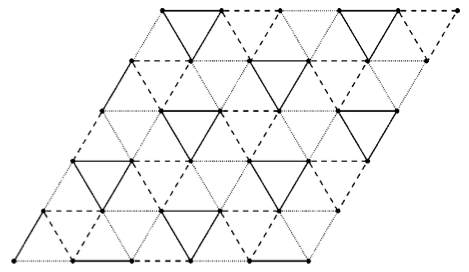
Figure 24: Triangular lattice on which the effective Hamiltonian is defined. The unitary vector for the bond is indicated by solid lines (${\bf e}_{\mu}={\bf e}_{1}$), dashed lines (${\bf e}_{\mu}={\bf e}_{2}$), and dotted lines (${\bf e}_{\mu}={\bf e}_{3}$). From Ferrero et al. (2003).

Explicitly, the effective low energy Hamiltonian reads Ferrero et al. (2003); Capponi et al. (2004)

$$H=\frac{J^{\prime}}{9}\sum_{\langle ij\rangle}{\bm{\sigma}}_{i}\cdot{\bm{\sigma}}_{j}(1-4{\bf e}_{ij}\cdot{\bm{\tau}}_{i})(1-4{\bf e}_{ij}\cdot{\bm{\tau}}_{j}).$$ (126)

V.4.2 Uniform Kagome Antiferromagnet

Several groups Budnik & Auerbach (2004); Capponi et al. (2004) employed the “contractor renormalization method” (CORE) to investigate kagome antiferromagnets. This method has been invoked to find an effective low energy Hamiltonian for the uniform kagome antiferromagnet wherein all exchange couplings are the same. In a spirit similar to that earlier, the individual triangular units are examined and, to lowest order in CORE, an effective low energy Hamiltonian is constructed that embodies interactions between different triangular units. A notable difference with the earlier approach is that perturbation theory was not invoked. Rather the system is solved on larger size units and effective Hamiltonians involving the more primitive basic units are constructed. In Budnik & Auerbach (2004), a related yet, by comparison to Capponi et al. (2004); Ferrero et al. (2003), different definition of the spin and chiral degrees of freedom is employed. Rather explicitly, with $s$ an $S_{z}$ eigenvalue of a spin operator ${\bf S}$ and $\Uparrow$ and $\Downarrow$ denoting states of eigenvalues $\pm 1/2$ of a pseudo-spin operator ${\bf T}$, Budnik & Auerbach (2004)

$$|s,\Uparrow\rangle = \frac{|s\uparrow\downarrow\rangle-|s\downarrow\uparrow\rangle}{\sqrt{2}},$$

$$|s,\Downarrow\rangle = \frac{|s\uparrow\downarrow\rangle+|s\downarrow\uparrow\rangle}{\sqrt{6}}-\sqrt{\frac{2}{3}}|(-s)ss\rangle.$$ (127)

As in the perturbative treatment, the resulting effective Hamiltonian Budnik & Auerbach (2004) contains effective interactions similar to those of the Kugel-Khomskii model augmenting standard spin exchange and pseudo-spin exchange. These are further augmented by direct compass type interactions (i.e., pseudo-spin interactions uncoupled from spin) similar to those that arise from Jahn-Teller interactions in orbital systems as well as non-trivial compass type coupled pseudo-spin spin interactions of the form

$${\bf S}_{i}\cdot{\bf S}_{j}(J_{1}{\bf T}_{i}\cdot{\bf e}_{ij}+J_{2}{\bf T}_{j}\cdot{\bf e}_{ji})$$ (128)

with $J_{1}$ and $J_{2}$ being fixed multiples of the uniform exchange constant $J$ in the kagome lattice antiferromagnet. The direct pseudo-spin interactions that couple the chiralities on neighboring triangles favor the formation of aligning singlets parallel to one another along particular directions.

VI Symmetries of Compass Models

VI.1 Global, Topological, and Intermediate symmetries and invariances

In terms of symmetries, compass systems are particularly rich. In what follows, we will discuss the invariances that these systems exhibit, but first recall the classification of orders and their relation to symmetry:

(i) Global symmetry. In many condensed matter systems (e.g. ferromagnets, liquids), there is an invariance of the basic interactions with respect to global symmetry operations (e.g. continuous rotations in the case of ferromagnets, uniform translations and rotations in liquids) that are to be simultaneously performed on all of the constituents of the system. At sufficiently low temperatures (or strong enough interactions), such symmetries might be spontaneously broken.

(ii)Topological invariants and orders. Topological orders have been the object of some fascination in more recent years Wen (2004). In the condensed matter community, part of the activity in analyzing these types of order is stimulated by the prospects of tolerant free quantum computation – an issue which we will return to in Sec. X. What lies at the crux of topological order is the observation is that even if, in some cases, global symmetry breaking cannot occur, systems may nevertheless still exhibit a robust order of a non-local, topological, type.

The most prominent examples of topological order – long studied by high energy theorists – are afforded by gauge theories Kogut (1979); Wen (2004). Gauge theories display local gauge symmetries and indeed, in pure gauge theories – theories that have only gauge bosons yet no matter sources – the only measurable quantities pertain to correlators defined on loops, the so-called Wilson loops. Related products pertain to open contours in some cases when matter sources are present Kogut (1979); Fradkin & Shenker (1979); Nussinov (2005).

(ii)Intermediate symmetry. The crucial point is that many compass systems display symmetries which, generally, lie midway between the above two extremes of global symmetries and local gauge symmetries. To make this statement precise, one can rephrase it in a formal way as it applies to general systems Batista & Nussinov (2005); Nussinov et al. (2012b). Consider a theory with fields $\{\phi_{\bf i}\}$ that is characterized by a Hamiltonian $H$ (or action $\cal{S}$).

Definition: A $d$-dimensional gauge-like symmetry of a theory is a group of symmetry transformations such that the minimal non-empty set of fields $\{\phi_{\bf i}\}$ changed by the group operations occupies a $d$-dimensional subset ($\cal{C}$) of the the full $D$-dimensional region on which the theory is defined. In the following we will refer to such symmetries as $d$-dimensional symmetries.

To exercise this notion it is useful to make contact with known cases. Clearly local gauge symmetries correspond to symmetries of dimension $d=0$. That is, gauge transformations can be applied locally at any point in space – a region of dimension $d=0$. At the opposite extreme, e.g., in a nearest neighbor ferromagnet on a $D$-dimensional lattice, described by the Heisenberg Hamiltonian $H=-J\sum_{\langle ij\rangle}{\bm{S}}_{i}\cdot{\bm{S}}_{j}$, the system is invariant under a global rotation of all spins. As the volume influenced by the symmetry operation occupies a $D$-dimensional region and in this case $d=D$. Sections VI.4, VI.5, VI.6, VI.7, VI.8 exemplify how symmetries of intermediate dimension $0<d<D$ arise in compass systems.

In their simplest form, one which typically appears in compass models, $d-$ dimensional symmetries are of the form

$$\prod_{j\in P}g_{j}$$ (129)

where $g_{j}$ are group elements associated with a site $j$ and $P$ is a $d-$ dimensional spatial region. In many cases, depending on the boundary conditions of the system, $P$ correspond to entire open $d-$ dimensional planes (as in 90^∘ compass models that we will review in subsection VI.4; see, e.g., Fig. 25) or closed contours (when compass models are endowed with periodic boundary conditions). Defect creation operators (those that restore symmetries) and translations of defects are typically products of local group elements that do not span such an entire region $P$ but rather a fragment of it (see, e.g., the open finite string in Fig. 25 with domain wall boundaries) generally leading to defects at the boundaries where the group element operations are applied Nussinov & Ortiz (2009c). We will pay particular attention to defect creation operators in the Kitaev compass model in Section X when we will discuss anyons and how they can be moved.

VI.2 Exact and Emergent Symmetries

A Hamiltonian $H$, and by extension the system it describes, can have two principal kinds of symmetries: exact and emergent ones. These are defined as follows.

(i) Exact symmetries. By this, one refers to the existence operators ${\hat{O}}$ that commute with the Hamiltonian

$$[H,{\hat{O}}]=0.$$ (130)

Such operators, indicted in this review by a hat $\hat{}$, reflect symmetries of the Hamiltonian.

(ii) Emergent symmetries. In many compass (and numerous other) systems, there are operators $\tilde{O}$ that do not commute with the Hamiltonian,

$$[H,\tilde{O}]\neq 0$$ (131)

i.e., do not satisfy Eq. (130) and are therefore indicated throughout this review by a tilde $\tilde{}$. Yet these operators do become symmetries when projected to a particular sector – a particular subset of states on which the Hamiltonian acts. That is,

$$[H,{\cal{P}}\tilde{O}{\cal{P}}]=0,$$ (132)

where ${\cal{P}}$ is the relevant projection operator that sector. In this case, if one defines ${\cal{P}}\tilde{O}{\cal{P}}={\hat{O}}$ then ${\hat{O}}$ will be an exact symmetry satisfying Eq. (130).

The most prominent cases in condensed matter systems, compass models in particular, relate to symmetries that appear in the ground state sector alone. In such instances, the symmetries are sometimes said to emerge in the low energy sector of the theory.

Although the formulation above is for quantum Hamiltonians, the same can, of course, be said for classical systems. There are numerous classical systems in which the application of a particular operation on an initial configuration will yield, in general, a new configuration with a differing energy. However, when such an operation is performed on a particular subset of configurations, such as the classical ground states, it will lead to other configurations that have precisely the same energy as the initial state. Similarly, certain quantum systems exhibit such particular symmetries only in their large pseudo-spin (or classical) limit. In such cases, symmetries may be said to emerge in the large pseudo-spin (or classical) limit. As will be reviewed in sections VI.4.3, VI.5, VI.6, particularly in certain compass-type models, symmetries may emerge within a sector of the combined large pseudo-spin and/or low energy (or temperature) limit.

One should note that emergent low-energy symmetries are notably different from the far more standard situation of spontaneous symmetry breaking, wherein an invariance of the Hamiltonian (or action) is spontaneously broken in individual low energy states (which are related to one other by the symmetry operation at hand). In the condensed matter arena, the canonical example is rotationally symmetric ferromagnets in a spatial dimension larger than three, in which at sufficiently low temperature a finite magnetization points along a certain direction – thus breaking the rotational symmetry. Another canonical example is the discrete (up $\leftrightarrow$ down or) time reversal symmetry is broken in Ising ferromagnets. Spontaneous symmetry breaking appears in systems that exhibit long-range order of some sort such as crystallization (breaking translational and rotational symmetries), superconductors (local gauge invariance and a Anderson-Higgs mechanism), superfluid Helium. Other examples include the Higgs mechanism of particle physics, chiral symmetry breaking in quantum chromodynamics, nucleon pairing in nuclei, electro-weak symmetry breaking at low energies, and related mass generation.

In all of these textbook examples, the system is symmetric at high energies and exhibits low-energy states that do not have that symmetry. However, in low energy emergent symmetries, the situation is reversed: the system may become more symmetric in the low-energy sector. We will discuss explicit examples of exact and emergent symmetries in compass models in the following sections.

VI.3 Consequences of Intermediate Symmetry

In this subsection, we review the consequences of intermediate symmetries. In later subsections, we will see how these the intermediate symmetries the below features appear in various compass models. Aside from the earlier results reviewed below, in Section VII, we will further report on a new consequence concerning the link between these symmetries and “flat bands” and illustrate how this relation appears throughout the compass models investigated.

VI.3.1 Degeneracy of Spectrum

We now briefly discuss how the presence of a $d$-dimensional intermediate symmetry, either classical or quantum, implies an exponential degeneracy of the energy spectrum that corresponds to the Hamiltonian. The application of intermediate symmetries on disparate $d$-dimensional planes leads to inequivalent states that all share the same energy. If a symmetry transformation $\tilde{O}_{P}$ has its support on a $d$-dimensional plane $P$, then one can concoct the composite symmetry operators

$$\tilde{O}_{composite}=\tilde{O}_{P_{1}}\tilde{O}_{P_{2}}..\tilde{O}_{P_{R}}.$$ (133)

For a hypercubic lattice in $D$ dimensions which is of size $L\times L\times L...\times L$, the number of independent planes ($R$) in Eq. (133) scales as $R={\cal{O}}(L^{d^{\prime}})$ where

$$d^{\prime}=D-d.$$ (134)

If each individual $d$-dimensional symmetry operation (exact or emergent) $U_{P_{i}}$ leads to a degeneracy factor of $m$ then the composite operation of Eq. (133) can lead to a degeneracy (of any state (for exact symmetries) or of the ground state (for emergent symmetries)) whose logarithm is of magnitude

$$\log_{m}{\sf degeneracy}={\cal{O}}(L^{D-d}).$$ (135)

That this is indeed the case is clearer for classical system with discrete symmetries than for quantum systems. Nevertheless, in the thermodynamic limit and/or on lattices whose boundaries are tilted the degeneracy factor of Eq. (135) associated with the intermediate $d$-dimensional symmetries becomes exact Nussinov & Shtengel (2013). On hypercubic lattices, such as the square lattice of the planar 90^∘ compass model discussed in subsection VI.4, whose boundaries are the same along the $d^{\prime}$ directions orthogonal to the planes $P$, the application of the operators of Eq. (133) does not lead to independent states for finite size systems. However, in the thermodynamic limit, the application of disparate operators of the form of Eq. (133) on a given initial state may lead to orthogonal states.

VI.3.2 Dimensional Reduction

The existence of intermediate symmetries has important consequences: it implies a dimensional reduction. The corresponding dimensional reduction is only with respect to expectation values of local quantities: the free energies of these systems and the transitions that they exhibit are generally those of systems in high dimensions Batista & Nussinov (2005); Nussinov et al. (2012b).

Theorem on Dimensional Reduction

More precisely, the expectation value of any such quantity $\langle f\rangle$ in the original system (of dimension $D$) is bounded from above by the expectation value of the same quantity evaluated on a $d$ dimensional region:

$$|\langle f\rangle|\leq|\langle f\rangle|_{H_{d}}.$$ (136)

The expectation value $\langle f\rangle$ refers to that done in the original system (or lattice) that resides in $D$ spatial dimensions. The Hamiltonian $H_{d}$ on the righthand side is defined on a $d$ dimensional subregion of the full lattice (system). The dimensionality $d\leq D$. The Hamiltonian $H_{d}$ preserves the range of the interactions of the original systems. It is formed by pulling out of the full Hamiltonian on the complete ($D$ dimensional) lattice, the parts of the Hamiltonian that appear within the $d$ dimensional sub-region ($\cal{C}$) on which the symmetry operates. Fields (spins) external to $\cal{C}$ act as non-symmetry breaking external fields in $H_{d}$. The bound of Eq. (136) becomes most powerful for quantities that are not symmetry invariant as then the expectation values $\langle f\rangle_{H_{d}}$ need to vanish for low spatial dimensions $d$ (as no spontaneous symmetry breaking can occur). This, together with Eq. (136), then implies that the expectation value of $\langle f\rangle$ on the full $D$ dimensional spatial lattice must vanish. By “non invariant”, we mean that $f(\phi_{\bf i})$ vanishes when summed over all arguments related to each other a $d$ dimensional symmetry operation, $\sum_{k}f[{\bf g}_{{\bf i}k}(\phi_{\bf i})]=0$. For continuous symmetries, non-invariance explicitly translates into an integral over the group elements $\int f[{\bf g}_{\bf i}(\phi_{\bf i})]d{\bf g}=0$.

We will now summarize for completeness general corollaries of such symmetry based analysis for general systems.

Corollaries

By choosing $f$ to be the order parameter or a two-particle correlator, one arrives at the following general corollaries Batista & Nussinov (2005); Nussinov et al. (2006, 2012b):

Corollary I: Any local quantity that is not invariant under local symmetries ($d=0$) or symmetries that act on one dimensional regions ($d=1$) has a vanishing expectation value $\langle f\rangle_{H_{d}}$ any finite temperature. This follows as both zero and one dimensional systems cannot exhibit symmetry breaking: in one and two dimensional systems, the expectation value of any local quantities not invariant under global symmetries: $\langle f\rangle=0$.

Physically, entropy overwhelms energetic penalties and forbids a symmetry breaking. Just as in zero and one dimensional systems, much more entropy is gained by introducing defects (e.g., domain walls in discrete systems), the same energy-entropy calculus is replicated when these symmetries are embedded in higher dimensions. An example with $d=1$ domain walls in a two-dimensional systems is afforded by the planar 90^∘ compass model [see Fig. 25]; even though the planar compass model is two-dimensional, the energy cost of these domain walls is identical to that in a $d=1$ system. The particular case of local ($d=0$) symmetry is that of Elitzur’s theorem Elitzur (1975) so well known in gauge theories. We may see it more generally as a consequence of dimensional reduction.

A discussion of how, by virtue of this consequence, such symmetries may protect and lead to topological quantum orders in systems at both finite and zero temperature appears in Nussinov & Ortiz (2009a, c).

Corollary II: One can push the consequences further by recalling that no symmetry breaking occurs for continuous symmetries in two spatial dimensions. Here again, free energy penalties are not sufficiently strong to induce order. When embedding continuous two dimensional symmetries in higher dimensions, the energy entropy balance is the same and the same result is attained $\langle f\rangle=0$ at all finite temperatures for any quantity $f$ that is not invariant under continuous $d\leq 2$ symmetries.

Further noting that order does not exist in continuous two dimensional systems also at zero temperature in the presence of a gap between ground and the next excited state, one similarly finds that for a $d\leq 2$ dimensional continuous symmetry the expectation value of any local quantity not invariant under this symmetry, strictly vanishes at zero temperature. Though local order cannot appear, multi-particle (including topological) order can exist. In standard gauge ($d=0$) theories, the product of gauge degrees of freedom along a closed loop (the Wilson loop) can attain a non-zero value as it may be invariant under all $d=0$ symmetries. In more general theories with higher $d$ dimensional symmetries, similar considerations may lead to loop (or “brane”) type correlators that involve multiple fields and are invariant under all low dimensional symmetries. As we will discuss in Section X, precisely such non-local correlation functions appear in Kitaev’s honeycomb model and many other systems with topological orders Chen & Nussinov (2008); Nussinov & Ortiz (2009c, a); Perez-Garcia et al. (2008).

In section VIII, we will review how when it is indeed allowed by symmetry, symmetry breaking in the highly degenerate compass models often transpires by a fluctuation driven mechanism (“order by disorder”) Villain (1972); Shender (1982); Henley (1989). In this mechanism, entropic contributions to the free energy play a key role.

Corollary III: Not only can one make statements about the absence of symmetry breaking, we can also adduce fractionalization of non-symmetry invariant quantities in high dimensional system. That occurs if no (quasi-particle type) resonant terms appear in the lower dimensional spectral functions Nussinov et al. (2006).

This corollary allows for fractionalization in quantum systems, where $d=1,2$. It enables symmetry invariant quasi-particles excitations to coexist with non-symmetry invariant fractionalized excitations. Fractionalized excitations may propagate in $(D-d)$ dimensional regions. Examples afforded by several frustrated spin models where spinons may drift along lines on the square lattice Batista & Trugman (2004) and in $D$ dimensional regions on the pyrochlore lattice Nussinov et al. (2007).

In what follows, we explicitly enumerate the symmetries that appear in various compass models. The physical origin of dimensional reduction in these systems can be seen examining intermediate symmetry restoring defects.

VI.4 Symmetries of the 90^∘ Compass Model

We now classify symmetries of the 90^∘ compass model in various spatial dimensions, reviewing both quantum and classical versions. To highlight some aspects of the symmetries of this system, it is profitable to discuss the general anisotropic compass model, as given for $D=2$ in Eq. (1) with general couplings $J_{x}$ and $J_{y}$ and in general spatial dimension $D$ given by Eq.(6), without field:

$$H^{90^{\circ}}_{D\square}=-\sum_{i,\gamma}J_{\gamma}\tau^{\gamma}_{i}\tau^{\gamma}_{i+\bm{e}_{\gamma}}.$$ (137)

The equivalent classical Hamiltonian on a $D$-dimensional hyper cubic lattice is

$$H^{90^{\circ}{\rm,class}}_{D\square}=-\sum_{i,\gamma}J_{\gamma}T^{\gamma}_{i}T^{\gamma}_{i+\bm{e}_{\gamma}}.$$ (138)

In the quantum systems, $T^{\gamma}$ are generators of the representations of SU(2) of size $(2T+1)$. For a pseudo-spin 1/2 system, $T^{\gamma}=\tau^{\gamma}/2$. In the classical arena, $T^{\gamma}$ are are the Cartesian components of normalized vector ${\bm{T}}$, as discussed in subsection III.2. These classical and quantum Hamiltonian systems exhibit both exact and emergent symmetries.

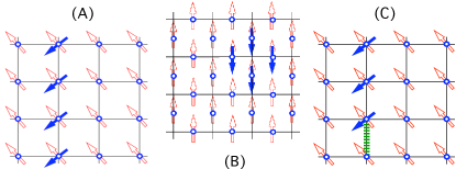
Figure 25: (A) The $90^{\circ}$ square lattice compass model. The action of the $d=1$ symmetry operation of Eq. (139) when the ”plane” $P$ is chosen to lie along the vertical axis. (B) A $d=0$ (local) gauge symmetry. Defects within a gauge theory cost a finite amount of energy. Local symmetries such as the one depicted above for an Ising lattice gauge theory cannot be broken. (C) A defect in a semi-classical ground state of the two dimensional orbital compass model. Defects such as this do not allow for a finite on-site magnetization. The energy penalty for this defect is finite (there is only one bad bond- the dashed line) whereas, precisely as in $d=1$ Ising systems, the entropy associated with such defects is monotonically increasing in system size Nussinov & Ortiz (2009c). Reproduced with permission.

VI.4.1 Exact discrete intermediate symmetries

Exact symmetries of both the square lattice and cubic lattice 90^∘ compass model in any pseudo-spin representation are given by Batista & Nussinov (2005); Nussinov et al. (2004); Biskup et al. (2005); Doucot et al. (2005); Nussinov & Fradkin (2005); Dorier et al. (2005)

$$\hat{O}^{(\gamma)}=\prod_{i\in P_{\gamma}}e^{i\pi T^{\gamma}_{i}}\,$$ (139)

where, as in Eq. (142), $P_{\gamma}$ is any line (in the case of the two-dimensional model) or plane (in the case of the cubic lattice model) which is orthogonal to the external ${\bf{e}_{\gamma}}$ axis of the lattice. A schematic for the $D=2$ dimensional case is provided in panel (a) of Fig. 25.

Albeit appearances, Eq. (139) is, when written longhand, quite different from Eq. (142). In Eq. (142) describing the emergent symmetries of the 120^∘ model, ${\bm{T}}$ is a two-component vector that is projected along three different equidistant non-orthogonal planar directions. That is, in Eq. (142), the unit vectors ${\bf{e}}_{\gamma}$ in the argument of the exponential correspond, with $\gamma=1,2,$ and $3$ to the equidistant non-orthogonal internal pseudo-spin directions ${\bm{a}},{\bm{b}},$ and ${\bm{c}}$ that lie in the two-dimensional plane defined of the 120^∘ model. By contrast, in Eq. (139), ${\bm{T}}$ is a $D=2$ (square lattice model) or $D=3$ (cubic lattice) vector and $T^{\gamma}$ are projections along orthogonal directions. The two operators appearing in Eqs. (142, 139) differ from one another: ${\bm{T}}\cdot{\bm{b}}\neq T_{2}$, etc. In Fig. (25), we provide a classical schematic of the action of such an operator when it acts on a uniform state. As in the case of the 120^∘ model on the cubic lattice, these operators lead to stratified states.

The exact nature of the symmetries of Eq. (139) is readily seen: the operators of Eq. (139) commute with the general Hamiltonian of Eq. (138): $[O^{(\gamma)},H]=0$. Thus, rotations of individual planes about an orthogonal axis leave the system invariant. Written generally, for a 90^∘ compass model in $D$ dimensions, the planes $P_{\gamma}$ are objects of spatial dimensionality $d=(D-1)$. In the $D=3$ dimensional system, the symmetries of Eq.(139) are of dimension $d=2$ as the planes $P_{\gamma}$ are two-dimensional objects. On the square lattice, the symmetries are of dimension $d=1$ as $P_{\gamma}$ are lines. These symmetries hold for both the quantum system with arbitrary size pseudo-spin as well as the classical system of Eq. (43) in a high number of dimensions $D$. A consequence of these symmetries is an exponential in $L^{D-1}$ degeneracy of each eigenstate of the Hamiltonian (including but not limited to ground states) is, in systems with “tilted” boundary conditions that emulate the thermodynamic limit Nussinov & Shtengel (2013). In pseudo-spin one half realizations of this system [Eq.(137)], on an $L\times L$ square lattice, a $2^{L}$ degeneracy was numerically adduced for anisotropic systems ($J_{x}\neq J_{y}$) in the thermodynamic limit Dorier et al. (2005).

Now, here is an important point to which we wish to reiterate- that of the physical origin of the dimensional reduction in this system. In a $D=2$ dimensional 90^∘ compass model system, the energy cost for creating defects (domain walls) is identical to that in a $d=1$ dimensional system [see Fig. 25]. With the aid of the bound of Eq. (136), we then see the finite temperature expectation value $\langle\sigma^{z}_{i}\rangle=0$ within the $D=2$ orbital compass model. The physical engine behind the loss of on-site order of $\langle\sigma^{z}_{i}\rangle$ is the proliferation of solitons, see Fig. 25. Just as in $d=1$ dimensional systems, domain walls (solitons) cost only a finite amount of energy while their entropy increases with system size. A schematic is provided in panel (c) of Fig. 25. The Hamiltonian $H_{d=1}$ defined on the vertical chain of Fig. 25 where these operations appear is none other than a one dimensional Ising Hamiltonian augmented by transverse fields generated by spins outside the vertical chain. Any fixed values of the spins outside the $d=1$ dimensional chain lead to transverse fields that act on the chain. These along the Ising exchange interactions between neighboring spins along the chain lead in this case to the pertinent $H_{d=1}$ in Eq. (136): that of a transverse field Ising model Hamiltonian. By virtue of their location outside the region where the symmetry of Eq. (139) operates, the spins $\sigma^{x}_{i\not\in P_{x}}$ do not break the discrete $d=1$ symmetry associated with the plane $P_{x}$. These defects do not enable a finite temperature symmetry breaking.

VI.4.2 Exact discrete global symmetries

When the couplings are not completely anisotropic (e.g., $J_{x}=J_{y}\neq J_{z}$ or $J_{x}=J_{y}=J_{z}$ on the cubic lattice or $J_{x}=J_{y}$ on the square lattice) there are additional discrete symmetries augmenting the $d=D-1$ Ising symmetries detailed above. For instance, when $J_{x}=J_{y}\neq J_{z}$ a global discrete rotation of all pseudo-spins on the lattice by an angle of 90^∘ about the $T^{z}$ direction leaves the Hamiltonian of Eq. (138) invariant. Such a discrete rotation essentially permutes the $x$ and $y$ oriented bonds which are all of equal weight in the isotropic case when these are summed over the entire square lattice. The same, of course, also applies for the square lattice model when $J_{x}=J_{y}$.

Yet another possible representation of essentially the same symmetry as it is pertinent to the exchange of couplings in the compass model is that of a uniform global rotation by 180^∘ about the $(1/\sqrt{2},1/\sqrt{2})$ direction of the pseudo-spins. Such a representation will return in Eq. (160) later on. Similarly, when $J_{x}=J_{y}=J_{z}$, a uniform global rotation by 120^∘ of all pseudo-spins about the internal $(1/\sqrt{3},1/\sqrt{3},1/\sqrt{3})$ pseudo-spin direction is also a discrete symmetry; this latter symmetry is of the $Z_{3}$ type- if performed three times in a row, this will give back the identity operation.

These additional discrete symmetries endow the system with a higher degeneracy. For isotropic systems ($J_{x}=J_{y}$), numerically a $2^{L+1}$ fold degeneracy is seen in the pseudo-spin $T=1/2$ system Dorier et al. (2005); this additional doubling of the degeneracy is related to a global Ising operation of a rotation by 180^∘ about a chosen pseudo-spin direction that leaves the system invariant. These additional symmetries are global symmetries and thus of a dimension $d=D$ which is higher than that of the discrete lower dimensional that are present in both the anisotropic and isotropic systems ($d=(D-1)$). As a result, in, e.g., the isotropic $D=2$ dimensional 90^∘ compass model may exhibit a finite temperature breaking of such a discrete global symmetry associated with such a discrete rotation. By contrast, the $d=1$ symmetries of the two-dimensional 90^∘ compass model cannot be broken as will discussed in section VI.3.2.

We note that in the classical anisotropic rendition of this system the degeneracy is exactly the same- i.e., $2^{L}$, aside from continuous emergent symmetries that will be discussed in the next section. The classical isotropic case is somewhat richer. There, each uniform pseudo-spin state (each such state is a ground state as will be elaborated in section (VII) and there is an additional degeneracy factor of $2^{2L}$ associated with the $2L$ independent classical $d=1$ Ising symmetries.

VI.4.3 Emergent Intermediate Discrete Symmetries: Cubic 90^∘ Model

We now turn to intermediate symmetries that appear in the large pseudo-spin (or classical) limit of the 90^∘ compass model in three dimensions. In its classical limit, the classical 90^∘ compass model on the cubic lattice has $d=1$ inversion (or reflection) symmetries along lines parallel to each of the three Cartesian axes $x_{a}$. Along these lines, we may set $\tau^{a}_{i}\to-\tau^{a}_{i}$ and not touch the other components. This corresponds to, e.g, a reflection in the internal $xy$ pseudo-spin plane when we invert $\tau^{z}$ and not alter the $x$ or $y$ components.

We explicitly note that this transformation is not canonical and does not satisfy the commutation relation and is thus disallowed quantum mechanically; indeed, this appears only as an emergent symmetry in the classical limit of large pseudo-spin. Instead in the 90^∘ compass model on the cubic lattice, quantum mechanically we have the $d=2$ symmetries which we wrote earlier (which of course trivially also hold for the classical system). Thus, the quantum system is less symmetric than its classical counterpart.

By contrast to the cubic lattice case, for the square lattice 90^∘ compass model, the intermediate $d=1$ symmetries of Eqs. 139 are are exact quantum (as well as classical) symmetries.

VI.4.4 Emergent Continuous Global Symmetries

In addition to its exact symmetries, the 90^∘ model also exhibits emergent symmetries in its isotropic version. As mentioned earlier, globally uniform pseudo-vector configurations are ground states of any classical isotropic ferromagnetic compass model. Thus, similar to the considerations presented for the 120^∘ compass model, any global rotation of all pseudo-spins is an emergent symmetry of the 90^∘ models. In the $D=2$ system, this corresponds to a global $U(1)$ rotation of all angles of the planar pseudo-spins. In the $D=3$ cubic lattice system, any SO(3) rotation of the three-dimensional pseudo-spins is an emergent symmetry. That a rotation does not change the energy of any uniform configuration is clear in the 90^∘ model. Imagine that all pseudo-spins in the planar 90^∘ model are oriented at an angle $\theta$ relative to the $T^{x}$ axis. In such a case, the energy associated with the horizontal bonds, $T^{x}_{i}T^{x}_{i+{\bm{e}}_{x}}$ will vary as $\cos^{2}\theta$ whereas that associated with the vertical bonds varies as $\sin^{2}\theta$. As $J_{x}=J_{y}=J$ in the isotropic system and as $\sin^{2}\theta+\cos^{2}\theta=1$, any uniform pseudo-spin state will have the same energy (which is, in fact, the ground state energy as we be discussed in section VII.1) and global rotations will not alter this energy.

VI.5 Emergent Symmetries: Classical Cubic 120^∘ Compass Model

The 120^∘ compass model on a 3D cubic lattice, Eqs.(19, 23), exhibits non-trivial symmetries which emerge in the ground state sector in the large pseudo-spin $T$ (classical) limit Lieb (1973); Simon (1980) (see also section III.2). In the classification of section VI.2, all of the symmetries which we detail below correspond to emergent symmetries. Before explicitly describing these symmetries, we briefly recount how to define this classical system from the quantum one, which we briefly alluded to in subsection V.1.6.

The classical 120^∘ compass model may, following the discussion in subsection III.2, be specified as follows. At each site we assign a unit length two-component spin denoted by ${\bm{T}}$. Let $\bf{a}$, $\bf{b}$ and $\bf{c}$ be evenly-spaced vectors on the unit circle that are separated from one another by 120 degrees. To conform with the operators of Eq. (19), one sets $\bf{c}$ to point at $0^{\circ}$ and $\bf{a}$ and $\bf{b}$ to be at $\pm 120^{\circ}$, respectively. Next, one defines $T^{(c)}={\bm{T}}\cdot{\bm{c}}$, and similarly for $T^{(a,b)}$. These projections onto the above unit vectors, $T^{(a,b,c)}$, are the classical counterpart of the pseudo-spin 1/2 operators of Eq. (19). The classical 120^∘ compass model Hamiltonian is then given by

$$H_{3\square}^{120{\rm,class}}=-\sum_{i}\left(T_{i}^{(a)}T_{i+{\bf e}_{x}}^{(a)}+T_{i}^{(b)}T_{i+{\bf e}_{y}}^{(b)}+T_{i}^{(c)}T_{i+{\bf e}_{z}}^{(c)}\right),$$ (140)

where the interaction strength $J$ is set to unity. The ferromagnetic and antiferromagnetic model are related by symmetry, so that for convenience the interaction strength is chosen as negative, so that low-temeprature ordering patterns of pseudospins tend to be uniform. This model exhibits two types of emergent symmetries in its ground state sector.

VI.5.1 Emergent Continuous Global Symmetries

All uniform pseudo-spin configurations, i.e., ones with constant pseudo-spin ${\bm{T}}_{i}={\bm{T}}$ or uniform angular orientation of the classical two component pseudo-spins in the XY plane, are ground states of $H_{3\square}^{120{\rm,class}}$ in Eq.(140) Nussinov et al. (2004). Therefore any configuration for which

$$T^{\gamma}_{i}=T^{\gamma}_{i+\bm{e}_{\gamma}}$$ (141)

on all sites $i$ is also a ground state configuration. Thus, when the system is restricted to this subspace of uniform configurations, any uniform rotation of all of the pseudo-spin angles $\theta_{i}\to\theta_{i}+\delta\theta$ does not change the energy. This global rotation operation – formally a $U(1)$ symmetry – emerges as a symmetry when the system is restricted to these ground states. It can be readily verified that this emergent symmetry is not an exact symmetry of the system. When a global rotation is applied to any initial pseudo-spin configuration that is not uniform, it will generally lead to a new state that has an energy from that of the initial configuration.

Formally therefore the classical cubic lattice 120^∘ compass model exhibits a global (i.e., a dimension $d=D=3$) emergent U(1) symmetry within the ground state sector. It turns out that on top of this there are additional non-uniform stratified classical ground states for which this global rotation is not a symmetry, which will be discussed next.

VI.5.2 Emergent Discrete $d=2$ Symmetries

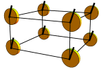
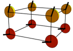
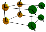
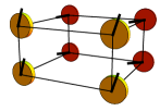
Figure 26: The symmetries of Eq. (142) applied a uniform ground state (top left).

The existence of a global rotational symmetry, as discussed in the previous section, is pervasive in physical systems – although usually these are exact symmetries. Much more peculiar to the 120^∘ compass and related models is the existence of numerous low dimensional ($d<D$) symmetries. These symmetries relate to ground states that will be stabilized at finite (yet low) temperatures. An explanation of what these symmetries are is given best done pictorially. In the top lefthand corner of Fig. 26, a general uniform configuration is shown – a ground state of the classical system. Starting with any such state, it is possible to reflect pseudo-spins in individual planes to generate myriad other configurations which are also ground states of the classical 120^∘ compass model. For instance, one may take any plane that is orthogonal to the ${\bf{e}}_{x}$ direction and reflect all of the pseudo-spins in that plane about the ${\bf a}$ direction. Under such an operation, $T_{i}^{(a}$ is unchanged but the pseudo-spin component along the direction that is orthogonal to ${\bf{a}}$ flips its sign. This will lead to a state that has exactly the same energy as that of the uniform state. Similarly, one may reflect all pseudo-spins in planes orthogonal to the ${\bf{e}}_{y}$ or ${\bf{e}}_{z}$ directions by ${\bf b}$ or ${\bf{c}}$ respectively. All of these three cases are depicted in Fig. 26.

These reflections are Ising symmetry operations or, formally, $Z_{2}$ symmetries. Any reflection performed twice will lead to the original state and is thus an Ising type operation. Going beyond the $2\times 2\times 2$ cube shown in Fig. 26, one can consider a cubic lattice of dimension $L\times L\times L$ with $L\gg 1$. On such a lattice, these reflections which are emergent ($d=2$) $[Z_{2}]^{3L}$ gauge-like symmetry operators Batista & Nussinov (2005); Nussinov et al. (2004); Biskup et al. (2005). The power of $(3L)$ relates to the number of planes ($d=2$ dimensional objects) in which such reflections can be applied: there are $L$ such planes which orthogonal to one of the three cubic lattice directions.

Formally, these operations, rotations of all pseudo-spins by an angle of 180^∘ about the internal $T^{\gamma}$ axis, can be written as quantum operators in the limit of large pseudospin size (where they correspond to classical rotations). These operations are

$$\tilde{O}^{(\gamma)}=\prod_{i\in P_{\gamma}}e^{i\pi{\bm{T}}_{i}\cdot{\bf{e}}_{\gamma}},$$ (142)

where $P_{\gamma}$ is any plane orthogonal to the corresponding cubic ${\bf{e}}_{\gamma}$ axis. It is important to re-iterate that these are not bona fide symmetries over the entire spectrum – these are not exact symmetries of the Hamiltonian. That is, these operations are symmetries when restricted to classical ground states and emerge in those combined limits, i.e., the classical limits of (i) high pseudo-spin and (ii) zero temperature.

It is well-known that two-dimensional Ising symmetries can be broken at finite temperatures. Thus, the symmetries of Eq. (142) of the classical 120^∘ can be broken. And indeed they are, as will be discussed in section VIII.2.1.

VI.6 Emergent Symmetries: Classical Honeycomb 120^∘ Compass Model

We will now review the ground states and associated low energy emergent symmetries of the classical (or large pseudo-spin limit of the) 120^∘ model on the honeycomb lattice Nasu et al. (2008); Zhao & Liu (2008); Wu (2008),. This model is given by Eq. (31). In what follows, we will invoke a decomposition of the honeycomb lattice into two interpenetrating triangular sublattices, referred to as sublattices A and B. Two neighboring sites of the honeycomb lattices thus belong to different sublattices.

The $120^{\circ}$ model on the honeycomb lattice shares a number of similarities with the 120^∘ model on the cubic lattice discussed above and the key elements of the discussion will be the same. Nevertheless, in some respects, this system is even richer largely as a result of the larger number of emergent symmetries in the ground state sector.

One may generally may seek to find all of the ground states of this system using Eq. (141) – a condition for finding all ground states of classical ferromagnetic compass model. It is instructive, within the framework of symmetries, to compare the consequences of this constraint as they apply to both the cubic lattice 120^∘ model whose symmetries we enumerated above and the honeycomb lattice 120^∘ model.

The coordination number of honeycomb lattice ($z=3$) is far smaller than that of the cubic lattice ($z=6$). Thus, the number of independent conditions of the type of Eq. (141) will be halved. As a result of this simple counting argument, we see that the ground state manifold might be far richer. This indeed turns out to be the case and emergent local ($d=0$) symmetries appear.

We first review the ground states of this classical system and stratification procedures that are more similar in nature to those of the 120^∘ model on the cubic lattice (i.e., involve the application of emergent intermediate and global symmetries on a uniform ground state) and then review additional local symmetry operations that appear in this case.

VI.6.1 Ground States and Emergent Intermediate Symmetries

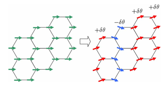
Figure 27: Left: pseudospin configuration for $\theta^{*}$=0. Right: configuration obtained by $\pm\delta\theta$ rotations of pseudospins in each zigzag chain. Nasu et al. (2008).

In the classical limit, the pseudo-spins in Eq. (31) become two-component (XY) type variables which may parameterized by (with some abuse of notation) a continuous angular variable $\theta_{i}$ at the different lattice sites $i$. Here, $\{\theta_{i}\}$ denote the orientation of the classical pseudo-vectors ${\bf T}_{i}$ (the large pseudo-spin limit variant of ${\bf\tau}_{i}$ in Eq. (31)).

As in the cubic lattice case reviewed in Sec. VI.5 all uniform states (${\bf T}_{i}={\bf T}$) are ground states and these may be stratified by the application of low dimensional emergent symmetry operations. The $d=2$ emergent symmetries of Eq. (142) and Fig. 26 have their counterparts in $d=1$ symmetries in the 120^∘ model on the honeycomb lattice Nasu et al. (2008). As shown in Fig. 27 it is possible, starting from a uniform state to generate other ground states by varying $\theta_{i}\to\theta_{i}+\delta\theta_{i}$. In this case, by considering (the $d=1$) zig-zag chains along one of the three crystalline directions Nasu et al. (2008), it is possible to generate other ground states by a reflection of all of the spins in these chains as in Fig. 27.

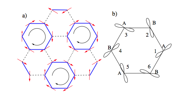
Figure 28: The fully packed oriented loop configurations in which $\tau$-vectors lie in directions of $\phi=\pm 30^{\circ},\pm 90^{\circ},\pm 150^{\circ}$. (a) The closest packed loop configuration with all the loops in the same chirality. (b) The p-orbital configuration for one closed loop in (a). The azimuthal angles of the p-orbitals are $45^{\circ},105^{\circ},165^{\circ},225^{\circ},285^{\circ},345^{\circ}$ Wu (2008).

VI.6.2 Emergent Local Symmetries

Fig. 28 shows particular ground states found by Wu (2008) wherein the pseudo-spins ${\bf T}_{i}$ are oriented in the plane, at angles of $(\pm 30^{\circ},\pm 90^{\circ},\pm 150^{\circ})$ such that they are tangential to the basic hexagonal plaquettes. In Fig. 28, the explicitly shown clockwise (or anti-clockwise) chirality [correspondingly, $C_{h}=1$ (or $C_{h}=-1$)] for each hexagon $h$ relates to the tangential direction of the pseudo-spins which can be flipped with no energy cost. Similar to our earlier considerations, chiral degrees of freedom in adhere to emergent discrete Ising like gauge symmetries (or $d=0$ symmetries in the classification of Section VI.1). These particular ground states lie within a larger space of classical states that are generated from the chiral tangential patterns is shown in Figs. 28,29. Panel (a) of Fig. 29 corresponds to a staggered rotation by 90^∘ of the chiral state depicted in Fig. 28. Generally, this larger set of ground states is generated by an application of a continuous $d=2$ symmetry on the ground states of Fig. 28. This set of classical configurations may be obtained as follows: Starting with any tangential state of the pseudo-spins an in Fig. 28 about the various hexagons, one can apply a global staggered ($U(1)$) rotation of all of the pseudo-spins in the plane such that all of the spins that lie on sublattice A are rotated by an angle of $\delta\theta$ whereas all of the spins lying on sublattice B are rotated by an angle of $(-\delta\theta$). This leads to state such as those shown in Fig. 29. Wu (2008) provides a detailed analysis of these results.

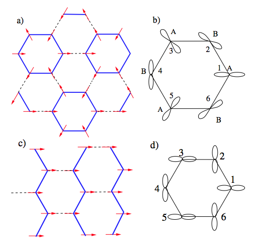
Figure 29: The fully packed unoriented loop configurations in which $\tau$-vectors lie along the bond directions. (a), (c) are the $\tau$-vector configurations with the closest packed loops and the ferromagnetic state, respectively. (b), (d) are their corresponding p-orbital configurations Wu (2008).

VI.7 Emergent Symmetries of the Triangular 120^∘ Compass Model

In its ground state sector, the classical 120^∘ model of Eq. (37) exhibits $d=1$ dimensional emergent symmetries. Similar to those discussed above, those relate to reflections of the pseudo-spins ($T_{i}^{\gamma}\to-T_{i}^{\gamma}$) for all sites $i$ that lie along a “plane” $P$ (a one-dimensional line in this case) that is parallel to the direction ${\bm{e}}_{\gamma}$. This operation leads to stratified states once again. A schematic is shown in Fig. 30.

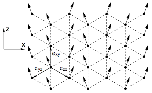
Figure 30: The triangular lattice formed in the $[111]$ plane. Shown is a disordered mean-field ground state, in which the isospins form lines parallel to the unit vector ${\bf e}_{xy}$, such that $\langle T_{j}^{z}\rangle$ is the same on all lattice sites, while the sign of $\langle T_{j}^{x}\rangle$ varies arbitrarily from line to line. Mostovoy & Khomskii (2002).

VI.8 Three component Kugel-Khomskii model

In sections (III.1,V.1.4), we discussed the Kugel-Khomskii (KK) model Kugel & Khomskii (1972, 1973, 1982). In particular, we reviewed underlying physics of this Hamiltonian in subsection V.1.4. Its most prominent version is that for two component pseudo-spins wherein the KK Hamiltonian describes the two $e_{g}$ levels (represented by two-component pseudo-spins). We now return to the three-component variant of this model that is more pertinent to three $t_{2g}$ orbital states We will label these as follows Harris et al. (2003):

$$|a\rangle\equiv|yz\rangle,\hskip 19.91684pt|b\rangle\equiv|xz\rangle,\hskip 19.91684pt|c\rangle\equiv|xy\rangle.$$ (143)

To make the discussion self-contained, we write anew the KK Hamiltonian in its general form and focus on its three-component pseudo-spin version. The KK Hamiltonian is given by

$$H=\sum_{\langle ij\rangle\parallel\gamma}H_{\rm orb}^{(\gamma)}(ij)\left({\bm{S}}_{i}\cdot{\bm{S}}_{j}+\frac{1}{4}\right).$$ (144)

Physically, ${\bm{S}}_{i}$ is the spin of the electron at site $i$ and $H_{orb}^{(\gamma)}(ij)$ are operators that act on the orbital degrees of freedom. For TM atoms arranged in a cubic lattice, wherein each TM atom is surrounded by an octahedral cage of oxygens, these operators are given by

$$H_{\rm orb}^{(\gamma)}(ij)=J\left(4\hat{\pi}_{i}^{\gamma}\hat{\pi}_{j}^{\gamma}-2{\hat{\pi}}_{i}^{\gamma}-2\hat{\pi}_{j}^{\gamma}+1\right),$$ (145)

where $\hat{\pi}_{i}^{\gamma}$ are pseudospin components, and $\gamma=a,b,c$ is the direction of the bond $\langle ij\rangle$. In the three-component realization that we wish to discuss now,

$$\hat{\pi}_{i}^{\gamma}=\frac{1}{2}\tau_{i}^{\gamma}.$$ (146)

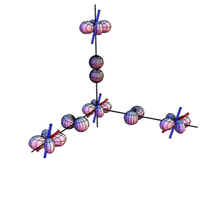
Figure 31: The anisotropic hopping amplitudes leading to the KK Hamiltonian after Ref. Batista & Nussinov (2005). The spins are indicated by blue rods. Similar to Ref. Harris et al. (2003), the four-lobed states denote the $3d$ orbitals of a TM ion while the intermediate small $p$ orbitals are oxygen orbitals through which the superexchange process occurs. Due to orthogonality with intermediate oxygen $p$ states, in any orbital state $|\gamma\rangle$ (e.g. $|c\rangle\equiv|xy\rangle$ above), hopping is disallowed between sites separated along the cubic $\gamma$ ($c$ above) axis. The ensuing KK Hamiltonian has a $d=2$ $SU(2)$ symmetry that corresponds to a uniform rotation of all spins whose orbital state is $|\gamma\rangle$ in any plane orthogonal to the cubic direction $\gamma$. Such a rotation in the $xy$ plane is indicated by the red spins in the figure.

The KK model in $t_{2g}$ systems exhibits a continuous exact lower dimensional symmetry as we now review. In the $t_{2g}$ compounds, hopping is disallowed via intermediate oxygen $p$ orbitals between any two electronic states of orbital flavor $|\gamma\rangle$ ($\gamma=a$, $b$, or $c$) along the $\gamma$ axis of the cubic lattice (see Fig. 31). As a consequence, as noted in Harris et al. (2003), a uniform rotation of all spins, whose electronic orbital state is $|\gamma\rangle$, in any plane ($P$) orthogonal to the $\gamma$ axis $c^{\dagger}_{i\gamma\sigma}=\sum_{\eta}U^{(P)}_{\sigma,\eta}d^{\dagger}_{i\gamma\eta}$ with $\sigma,\eta$ the spin directions, leaves Eq. (144) invariant. The total spin of electrons of orbital flavor $|\gamma\rangle$ in any plane orthogonal to the cubic $\gamma$ axis is conserved. Here, we have $d=2$ $SU(2)$ symmetries

$$\hat{O}_{P;\gamma}\equiv[\exp(i\bm{S}^{\gamma}_{P}\cdot{\bm{\theta}}^{\gamma}_{P})/\hbar],\hskip 28.45274pt[H,\hat{O}_{P;\gamma}]=0,$$ (147)

with $\bm{S}^{\gamma}_{P}=\sum_{i\in P}\bm{S}_{i}^{\gamma}$, being the sum of all the spins $\bm{S}^{i,\gamma}$ in the orbital state $\gamma$ in any plane $P$ orthogonal to the direction $\gamma$ (see Fig. 31).

We now, once again, turn to the physical origin of dimensional reduction in this system with continuous $d=2$ SU(2) symmetries. The bound of Eq. (136) prohibits, at finite temperatures, local on-site order is provided by Eq. (147) for the KK model. Physically, this is so due to the proliferation and deleterious effect of $d=2$ dimensional defects (i.e., spin waves) in SU(2) continuous pseudo-spin systems. The energy/entropy balance associated with these defects in the three-dimensional KK system is identical to that in a two-dimensional three-component Heisenberg spin system.

VII Intermediate Symmetries & Flat Bands in Classical Spin-wave Dispersion

In this section, we introduce a new result that will be of utility in understanding some aspects of the order-by-disorder physics and the role of the large degeneracy of these systems as it pertains to simple ${\bm{k}}$-space classical spin wave type analysis. We outline a new result that sheds light on the relation between spectral structure, degeneracy, and intermediate symmetries in general classical ferromagnetic compass systems in $D-$ spatial dimensions. In a nutshell, one asks what the consequences are of the existence of real-space stratified ground states found in section VIII [schematically illustrated in Figs. (26,27,28,30,31)] on the momentum space spectrum of pseudo-spin excitations. One finds that the low $d-$dimensional symmetries (either exact or emergent) that leads to the stratified states in real space their application on the canonical uniform (${\bm{k}}=0$) ferromagnetic state, lead, in momentum-space, to a redistribution of weights in $(D-d)$ dimensional regions. As all of these states share the same energy, one finds that the existence of $d$-dimensional symmetries ensures that there are $(D-d)$ dimensional volumes which are “flat” and share the same mode energy as the ${\bm{k}}=0$ point. Although $d$ dimensional symmetries imply flat bands in classical systems, the converse is not true- in classical systems with a finite number of pseudo-spin components, flat bands generally do not imply the existence of $d-$ dimensional symmetries. However, in the large $n$ limit, $(D-d)$ dimensional flat bands indeed imply the existence of $d-$ dimensional real space symmetries. Large $n$ analysis of these systems is identical to that of $d$ dimensional systems (i.e., in all directions orthogonal to the flat zero-energy regions in ${\bm{k}}$ space). That is, in the large $n$ system, an effective dimensional reduction occurs (from $D-$ dimensions to $d-$ dimensions). Thus, for systems with, e.g., $d=2$ symmetries (such as the cubic lattice 120^∘ compass model), large $n$ analysis and related approximate methods relying on simple classical ${\bm{k}}$-space spin wave analysis will, incorrectly, predict incorrectly that the finite $n$ classical system does not order and that quantum fluctuations are mandatory to explain the observed ordering in these systems. Similar considerations to all of these results concerning the interesting link between symmetries and band structure may apply, in general (i.e., not necessarily ferromagnetic) systems for both ground states and excited states.

VII.1 Uniform States as Ground States of Classical Compass Models

In the absence of an external field, the classical ground states corresponding to the general isotropic compass model Hamiltonian of Eq. (6) are fairly trivial. In the anisotropic (non-uniform $J_{\gamma}$), the pseudo-spins tend to align along the direction $\gamma^{\prime}$- the direction associated with the highest exchange coupling $J_{\gamma^{\prime}}$. We now first explicitly turn to the isotropic situation wherein $J_{\gamma}=J>0$ Nussinov et al. (2004); Biskup et al. (2005). As discussed in subsection III.2, in their classical rendition, the the pseudo-spins are normalized at all lattice sites, ${\bm{T}}_{i}^{2}=1$. In such a case, for the classical rendition all of the systems that we focus on in this review, up to an irrelevant additive constant $C$, the Hamiltonian may be written as a sum of squares

$$H_{isotropic}^{compass}=\frac{J}{2}\sum_{i}\left[\sum_{\gamma}(T^{\gamma}_{i}-T^{\gamma}_{i+\bm{e}_{\gamma}})^{2}-2C\right].$$ (148)

A direct computation shows yields the value of $C=\sum_{j}({\bm{T}}_{i}\cdot{\bm{e}}_{ij})^{2})$, which is independent of the orientation of ${\bm{T}}_{i}$. For all classical compass models on regular lattices with two-component (i.e., XY) type spins whose orientation may be specified by a single angle $\theta_{i}$ on the unit disk, the constant $C=z/2$ with $z$ being the coordination number of the lattice (the number of nearest neighbors of any given site). Values of the constant $C$ in Eq. (148) can be readily computed for compass models with a higher number of spin components. The classical $D-$ dimensional 90^∘ compass model of Eq. (43), the additive constant $C$ in Eq. (148) is given by $C=2$. Similarly, for the classical counterpart of the Kitaev model of Eq. (13), $C=1$.

As all terms in the sum of Eq. (148) are positive or zero, minima are achieved when ${\bf{T}}_{i}={\bf{T}}$ for all $i$ with ${\bf{T}}$ an arbitrary orientation. Thus, any uniform state is a ground state and a continuous global rotation may relate one such ground state to another. These rotations are not bona fide symmetries of the Hamiltonian and may emerge as such only in the restricted ground state subspace. Thus, the ferromagnetic compass models exhibit a continuous emergent symmetry of their ground states. Starting from any uniform state (a ground state of the classical system), any uniform global rotation of all pseudo-spins will lead to another ground state.

Although perhaps obvious, we remark on the relation between ferromagnetic and antiferromagnetic compass models. On bipartite lattices, the sign of the exchange couplings can be reversed ($J_{\gamma}\to-J_{\gamma}$) for classical systems. The same trivially holds true for quantum XY spins (such as those in the 120^∘ model) for which a canonical transformation (rotation by 180 degrees about the z axis) can be performed.

VII.2 Stratification in Classical Compass Models

The richness of the classical compass models stems from the many possible ground states that they may possess (aside from the uniform state). Such stratified ground states were depicted in Figs. (26,27,28,30,31). Equal energy states (classical or quantum) are generally related to each other via the symmetries discussed in Section VI.2. Emergent (and exact) symmetries of the classical ferromagnetic compass models link the uniform ferromagnetic states discussed in subsection VII.1 to a plethora of other classical ground states. As will be elaborated on in section VIII, this proliferation of low energy states lead to high entropic contributions and the failure of the simplest analysis to predict finite temperature order. We now explicitly determine all classical ground states of ferromagnetic compass models and link those to the earlier depicted ground states. As can be seen from Eq. (148), any configuration for which

$$T^{\gamma}_{i}=T^{\gamma}_{i+\bm{e}_{\gamma}}$$ (149)

on all sites $i$ is also a ground state configuration. That is, in standard compass models, the projections of any two nearest neighbor ${\bm{T}}$ along the bond direction $\gamma$ must be the same. [As noted several times earlier and made explicit in the original compass model definitions in subsection III.2, the components in Eq. (149) are defined by $T^{\gamma}\equiv{\bf{T}}\cdot{\bf{e}}_{\gamma}$; in this scalar product, the corresponding internal pseudo-spin unit vectors ${\bf{e}}_{\gamma}$ are chosen differently for different compass systems.] In Kitaev’s model, the direction specified by $\gamma$ is dictated by the lattice link direction but it is not equal to it. At any rate, generally, the number of conditions that Eq. (149) leads to is equal to the number of links on the lattice- $(Nz/2)$. Eq. (149) states that only the $\gamma$ component of the pseudo-spin ${\bf T}$ is important as we examine the system along the $\gamma$ lattice direction. It may therefore generally allow for numerous other configurations apart from the uniform ferromagnetic states in which one transforms the pseudo-spins in planes orthogonal to the $\gamma$ direction in such a way as not alter the projection $T^{\gamma}$ of ${\bf T}$ on the $\gamma$ axis. This allows for the multitude of ground states discussed in section(VI.2) that are related to the uniform ground states via intermediate low dimensional operation (generally an emergent symmetry of the ground state sector).

VII.3 Flat bands: Momentum Space Consequences of Real Space Stratified Ground States

A new prevalent aspect that has not been discussed before in the literature concerns a general relation between the classical ground states of the compass models and the classical spin wave dispersions. This new relation will be introduced shortly. Towards this end, it will be profitable to examine the matrix ${\hat{V}}({\bf k})$ of Eq. (56) in its internal pseudo-spin eigenbasis and write the classical compass Hamiltonians as

$$H=\frac{1}{2}\sum_{\alpha}\sum_{\bf k}v_{\alpha}({\bf k})|t_{\alpha}({\bf k})|^{2}.$$ (150)

In Eq. (150), the internal pseudo-spin space index $\alpha$ labels the eigenvalues $v_{\alpha}(\bf{k})$ of the matrix ${\hat{V}}({\bf k})$ and $t_{\alpha}({\bf k})$ are the internal pseudo-spin components of the vectors ${\bf T}({\bf k})$ when expressed in this basis.

These emergent symmetries within the ground state sector lead to an enormous degeneracy of the classical ground states. One can relate this to the eigenvalues of the matrix ${\hat{V}}({\bf k})$ of Eq. (56). Before doing so for the compass (and general systems), we reflect on the situation in canonical nearest neighbor classical ferromagnets. In standard, isotropic, ferromagnetic systems, $v_{\alpha}({\bf k})$ attains its global minimum when ${\bf k}=0$. Thus, in standard ferromagnets, only the uniform (${\bm{k}}=0$) states are ground states. Any other non-uniform state necessarily has non-vanishing Fourier space amplitudes $t_{\alpha}({\bf k})\neq 0$ also for modes ${\bm{k}}\neq 0$ each of which costs some energy relative to the lowest energy ${\bm{k}}=0$ state. By contrast, the multitude of non-uniform ground states generated by the stratification operations of Fig.  26 prove that $v_{\alpha}({\bf k})$ no longer attains its minimum at a single point in ${\bf k}$ space but rather at many such points. Applying the general stratification (or stacking) operations of, e.g., Fig. (26) on the uniform ${\bm{k}}=0$ state (one for which the Fourier amplitudes $T_{\bm{k}\neq 0}=0$ leads to new configurations for which the Fourier amplitudes $T_{\bm{k}}\neq 0$ where ${\bm{k}}$ lies along the $k_{z}$ axis.

According to Eq. (150), this suggests that the lowest values of $\min_{\alpha}\{v_{\alpha}({\bm{k}})\}$ define lines along the $k_{x}$, $k_{y}$, or $k_{z}$ axis. This can indeed be verified by a direct computation.

More generally, if, one sets $\min_{\alpha,{\bm{k}}}v_{\alpha}({\bm{k}})=0$ and the ground state energy happens to have a zero value according to Eq. (150) In general, of course, when one applies a general operation $U$ to get a new ground state, with $t_{\alpha^{\prime}}({\bm{k}^{\prime}})\neq 0$ then for all of these values of $\alpha^{\prime}$ and ${\bm{k}^{\prime}}$ with a non-zero Fourier amplitude $t_{\alpha^{\prime}}({\bm{k}^{\prime}})$, one must have that $v_{\alpha^{\prime}}({\bm{k}^{\prime}})=0$. The fact that the uniform ground states at ${\bf k}=0$ are invariant under global rotation (i.e., a change of basis of the internal indices $\alpha^{\prime}$ for all components $\alpha^{\prime}$ for which $t_{\alpha^{\prime}}({\bm{k}^{\prime}}=0)$) asserts that states having components $\alpha^{\prime}$ such that $\min_{\alpha}\{v_{\alpha}({\bm{k}}=0)\}=v_{\alpha^{\prime}}({\bm{k}}=0)$ can, indeed, be materialized. This follows as whatever $\alpha^{\prime}$ happens to be, for ${\bm{k}}=0$, the eigenvector ${\bm{t}}=(0..010...0)^{T}$ corresponding to it will relate to some particular uniform real space vector ${\bf{\tilde{T}}}$ in the original basis. On the other hand, any uniform state is a ground state and thus such a configuration with a vector ${\bf{\tilde{T}}}$ can be materialized. That is, the lower bound on the energy stemming from the lowest energy eigenvector(s) of $\hat{V}$ of Eq. (56) can be saturated.

Thus, emergent symmetries mandate the appearance of lines of nodes in the dispersion. [The same, of course, also trivially holds for exact symmetries of the Hamiltonian.] The converse is of course not true: the existence of flat regions of the dispersion (those with $v_{\alpha^{\prime}}({\bm{k}^{\prime}})=0$) do not mandate that symmetries appear in the ground state sector as although any linear combination involving only $t_{\alpha^{\prime}}({\bm{k}^{\prime}})$ it might not be possible to construct real space states out of these amplitudes for which ${\bm{T}}_{i}^{2}=1$ at all sites $i$.

The discussion above relates the degeneracies brought about by (exact or emergent) intermediate symmetries with the dispersion of $v_{\alpha}({\bf{k}})$ about its minimum. This general link between intermediate symmetries and (“flat”) spin-wave type dispersion applies to many of the other compass models in this review.

In general, if in a general compass model, a $d$ dimensional operation relates the different ground states (such as the $d=2$ reflections of Fig. (26) and Eq. (142) then the lowest bands $v_{\alpha}({\bm{k}})$ are zero (or, more generally attain their lowest values) within $d^{\prime}=(D-d)$ dimensional regions in $k-$space. This follows from the application, on a uniform ferromagnetic state of the symmetry operators of the form of Eq. (133). Different symmetries (either emergent ($\tilde{O}_{P}$) or exact ($\hat{O}_{P}$)) can be chosen in the string product of Eq. (133) that when acting on the uniform ferromagnetic state lead to disparate configurations that must all share the same energy. Thus, putting all of the pieces together, we have established a new theorem:

When a system of the general form of Eq. (150) exhibits a ferromagnetic state then the existence of $d$-dimensional symmetries (exact or emergent) implies that $v_{\alpha^{\prime}}({\bf k})$ has a flat dispersion in a $(D-d))$-dimensional manifold that connects to the ferromagnetic point of ${\bf k}=0$.

As explained above, for classical pseudo-spins ${\bf T}_{i}$ with a finite number ($n$) of components, that have to be normalized at each lattice site $i$, the converse is not guaranteed to be true: if one has flat lowest energy bands then we are not guaranteed that we can generate real space configurations with normalized pseudo-spins ${\bf T}_{i}$ whose sole Fourier amplitudes are associated with wave-vectors ${\bf k}$ that belong to these flat bands. In the large $n$ limit of the classical models (or, equivalently, in the corresponding spherical models) Berlin & Kac (1952); Stanley (1968); Nussinov (2001) the local normalization conditions becomes relaxed and linear superpositions of Fourier modes on the flat band lead to allowed states that share the same energy. That is, in the large $n$ limit (and, generally, only in that limit), if there is a band $v_{\alpha^{\prime}}({\bm{k}})$ that assumes a constant value $v_{\alpha^{\prime}}({\bm{k}})={\sf const.}$ for wave-vectors ${\bm{k}}$ that belong to a manifold ${\cal{M}}$ of dimension $d^{\prime}=D-d$ then the system exhibits a $d$-dimensional symmetry: any transformation that acts as a unitary transformation on the modes ${\bm{k}}\in{\cal{M}}$ will not alter the energy of states whose sole non-vanishing Fourier amplitudes $t_{\alpha^{\prime}}({\bm{k}})$ belong to this manifold. For related aspects, see Nussinov et al. (2012b); Batista & Nussinov (2005). As the spectrum $v_{\alpha^{\prime}}({\bm{k}})$ is pinned at its minimum value along $d^{\prime}=(D-d)$ dimensional regions in ${\bm{k}}$ space, large $n$ computations will, up to constant factors associated with the volume of these regions, reproduce results associated with the non-vanishing dispersion in the remaining $(D-d^{\prime})=d$ dimensional regions. Thus, in the large $n$ limit, the behavior of compass model ferromagnets in $D$ spatial dimensions is identical to that of the ferromagnets in the large $n$ limit in $d$ dimensions. As the large $n$ ferromagnet does not exhibit long range order in $d=2$ dimensions (and indeed any pseudo-vector system with $n\geq 2$ components), the large $n$ analysis of the classical cubic lattice 120^∘ model will predict that it does not order at finite temperatures- an erroneous conclusion. As it turns out, simple large $n$ and other related approximations are not valid for the analysis of the classical 120^∘ model and careful calculations are required for the free energy of the $n=2$ component classical system Biskup et al. (2005); Nussinov et al. (2004). We will return to this point in section VIII.2.1.

In principle, the theorem can be replicated for any other commensurate real space ground state structure for which the only non-vanishing Fourier components $t_{\alpha}({\bm{k}})\neq 0$ are those that minimize the kernel $v_{\alpha}({\bf k})$ in Eq. (150). In the above, we illustrated that the ferromagnetic compass model has, amongst many other states, the uniform (${\bm{k}}=0$) state as a ground-state. corresponding to well defined ${\bf k}$ space points. There are other commensurate structures (e.g., Neel states, 2 x 2 checkerboard states, etc.) that correspond to a particular set of wave-vectors Nussinov (2001). We proceed by discussing the particular realizations of this this theorem in compass models.

VII.3.1 Spin-waves of Cubic Lattice 120^∘ Compass Model

In the case of, e.g., the 120^∘ model in $D=3$ dimensions this co-dimension is $d^{\prime}=1$ and the zeros of the modes lie along lines (which happen to be the Cartesian coordinate axes in momentum space). We briefly remark that when local symmetry operations are present (i.e., when $d=0$) as they are on some of the more frustrated compass models that we will review later on then there will be flat bands where the corresponding $v_{\alpha^{\prime}}({\bm{k}})=0$ for all ${\bm{k}}$ in the full $(d^{\prime}=D)-$ dimensional $k-$ space for some value(s) of the (band) index $\alpha^{\prime}$.

Although it is, of course, of less physical significance, the analysis for the highest energy state is essentially identical to that for the ground states. When the sign in Eq. (149) may be flipped (as on bipartite lattices), the resulting staggered configuration is that of highest energy possible. Replicating all of the arguments made above mutatis mutandis it is seen that if the operations $U$ do not change the energy of these states then the manifold of highest energy modes is of the dimensionality $d^{\prime}$ of Eq. (134).

VII.3.2 Honeycomb Lattice 120^∘ Compass Model

We now discuss the system of Eq. (31) on the honeycomb lattice.

As was noted from Eq. (150), the existence emergent $d-$ dimensional symmetries of ground states that include the ferromagnetic state mandates (Eq. (134)) that a $d^{\prime}$ dimensional sub-volume of $k-$ space correspond to zero models ($v_{\alpha^{\prime}}({\bm{k}^{\prime}})=0$ for one of more bands $\alpha^{\prime}$).

Given the appearance of the discrete chiral $d=0$ symmetries above Wu (2008), given the earlier derivation above, one sees that $d^{\prime}=D$ and thus flat bands may exist corresponding to the highest and lowest possible energy states. Indeed, flat bands exist in the spin wave dispersion about a state that has these symmetries Wu (2008). A more general diagonalization of the $4\times 4$ matrix $\hat{V}(\vec{k})$ of Eq. (56) indeed illustrates that there are two-flat bands with (in our convention) values of $v_{1,2}({\bm{k}})=0,\frac{3J}{2}$ that correspond to the lowest and highest energies attainable. There are also two dispersing modes. [This matrix is of dimension four as a result of two factors or two. Translation invariance appears only for the honeycomb lattice once it is considered as a triangular lattice (belonging to either the A or B sublattices) with a basis of two sites. The second factor of two stems from the number of components of each of the classical pseudo-spin at each of these sites.

VIII Order by Disorder in Compass Models

In sections (VI, VII), we illustrated how classical (and also quantum) compass systems might exhibit numerous ground states. Aside from emergent global symmetries of the classical ferromagnetic compass model, both the classical and quantum models in $D$ spatial dimensions exhibit a degeneracy which scales exponentially in $L^{D-d}$ where $d$ is the dimension of the intermediate symmetries (see Eq. (135)). As we will now review, this large degeneracy is generally lifted by by fluctuations a process colloquially referred to as order-by-disorder Villain et al. (1980); Shender (1982); Henley (1989); Moessner (2000). Although several states may appear to be equally valid candidate ground state, fluctuations can stabilize those states which have the largest number of low energy fluctuations about them. These differences can be explicitly captured in values of the free energies for fluctuations about the contending states. Classically, fluctuations are driven by thermal effects and lead to entropic contributions to the free energy. Quantum tunneling processes may fortify such ordering tendencies (“quantum order by disorder” Henley (1989); Rastelli & Tassi (1987); Chubukov (1992)), especially so at zero temperature and stabilize a particular set of linear combinations of classically degenerate states. We note that albeit being very different, somewhat related physics concerning forces deriving from the weight of zero-point “fluctuations” appears in the well-known Casimir effect of quantum electro-dynamics Casimir & Polder (1948); Casimir (1948). In the classical arena, similar effects appear- sea farers have long known about the tendency of closely separated ships to pull inwards towards each other as a result of hydrodynamic fluctuations. Other notions related to those in order by disorder physics concern entropy driven effects that lead to particular conformations appear in the funnel model for protein folding Bryngelson et al. (1995).

VIII.1 Classical and Quantum Order out of Disorder

Colloquially, quantum and classical systems may be anticipated to exhibit the same qualitative “order out of disorder” physics. Although this is often the case, there is no fundamental reason for this to be so (and, indeed, the two effects may lead to very different results in some instances). Different sets of states can be stabilized by these fluctuations. An understanding of the quintessential physics may be obtained by considering small (harmonic) fluctuations about classical ground states. To harmonic order, within the quantum arena, the fluctuations will be governed by a Bose distribution (with frequencies $\omega_{i}$ that denote the energies of the various independent harmonic modes) whereas the classical fluctuations obey a Boltzmann distribution with the same set of harmonic modes. The two may, obviously, be radically different at low temperatures especially insofar as they apply to zero mode fluctuations about the ground states. In the appendix

In Appendix XV, section (VIII.2.1) [and in our discussion the large $n$ structure factor of the 120^∘ model] we will aim to make this intuition more precise. In a nutshell, in many situations, quantum systems may order more readily than their classical counterparts. This may, in some of the compass models that we consider. be viewed as a consequence of “order out of disorder” effects at play which can be more pronounced in quantum systems. We next examine order out of disorder effects in specific compass models.

VIII.2 Cubic lattice 120^∘ compass model

When entropic contributions are omitted, the spin-wave spectrum of the standard classical cubic lattice120^∘ compass model is gaplessvan den Brink et al. (1999b). This suggests that, on the classical level, these orbital systems exhibit finite temperature disorder. Indeed the commonly held lore for some time was that quantum fluctuations (tunneling between the different contending classical ground states) are mandatory in order to lift the orbital degeneracy and account for the experimentally detected orbital orders. Most of the work on “quantum order out of disorder” focused on $1/S$ corrections (with $S$ the spin size) to the classical spin-wave spectrum.

VIII.2.1 Thermal fluctuations

The difficulties encountered in the simplest analysis of the classical model stem from the $d=2$ symmetries that it exhibits [see section VI.2] as was exemplified in Fig. (26). As we discussed in subsection VII, these symmetries lead to flat $d^{\prime}=(D-d)$ dimensional regions in ${\bm{k}}$ space along which the dispersion $v_{\alpha^{\prime}}({\bm{k}})$ attains its minimum. In the case of the cubic lattice 120^∘ model, there are lines ($d^{\prime}=1$) along the Cartesian axis along which the dispersion is non-increasing. In simple Gaussian calculations (such as that of the large $n$ or spherical models) Biskup et al. (2005) this leads to a canonical divergent fluctuations that inhibit low temperature order. The divergences are identical to those associated with canonical $D-d^{\prime}=d$ ferromagnetic systems (or, in cubic lattice 120^∘ compass systems, those associated with two-dimensional continuous spin ferromagnetic systems). In various guises, this dispersion led to early difficulties in the analysis of this system and to the inclusion of quantum or thermal effects to lift this degeneracy. To make this lucid, we briefly note that the structure factor ${\cal{S}}({\bf k})$ within spin wave theory (and classical large $n$ analysis Biskup et al. (2005)) behaves, at low temperatures, as

$${\cal{S}}({\bf k})\propto\frac{E_{x}+E_{y}+E_{z}}{E_{x}E_{y}+E_{x}E_{z}+E_{y}E_{z}},$$ (151)

with the shorthand $E_{\gamma}({\bm{k}})\equiv 2-2\cos k_{\gamma}$. As can be seen by inspection, the structure factor of Eq. (151) diverges along lines in ${\bf k}$ space (corresponding to momenta along the lattice directions $k_{x}$, $k_{y}$, or $k_{z}$). As briefly alluded to in section VIII.1 [and elaborated on in the appendix], in the simplest, large $n$ spin-wave type approaches, this divergence of the classical system (as opposed to the convergence of the corresponding integral for its quantum large $n$ counterpart as well as standard $1/S$ calculations) leads to the false conclusion that there is no finite temperature ordering in this system. This divergence is removed by the proper inclusion of fluctuations about the ground states of the $n=2$ component classical pseudo-spin system- an item which we turn to next.

Let us now, in particular, briefly review finite temperature effects on the classical 120^∘-model of Eq. (140) Nussinov et al. (2004). The important thing to note is that the free energy minima (not the energy minima) determine the low energy states at finite temperatures. The classical spins $\{\vec{S}_{i}\}$ are parameterized by the angles $\{\theta_{i}\}$ with the $a$ axis. We may consider the finite temperature fluctuations about the uniform ground states where each $\theta_{i}=\theta^{\star}$. At low temperatures, the deviations $\vartheta_{i}=\theta_{i}-\theta^{\star}$ are small, and the quadratic [spin-wave (SW)] Hamiltonian corresponding to Eq. (140) becomes Nussinov et al. (2004); Biskup et al. (2005)

$$H_{\rm SW}=\frac{1}{2}\;J\sum_{i,\gamma}q_{\gamma}(\theta^{\star})\;(\vartheta_{i}-\vartheta_{i+\vec{e}_{\gamma}})^{2},$$ (152)

where $\gamma=a,b,c$ while $q_{c}(\theta^{\star})=\sin^{2}(\theta^{*})$, $q_{a}(\theta^{\star})=\sin^{2}(\theta^{\star}+2\pi/3)$ and $q_{b}(\theta^{*})=\sin^{2}(\theta^{\star}-2\pi/3)$. On a cubic lattice with periodic boundary conditions with  $\theta^{*}$ the average of $\theta_{i}$ on the lattice, at an inverse temperature $\beta=1/(k_{B}T)$, the partition function Nussinov et al. (2004); Biskup et al. (2005)

$$Z(\theta^{\star})=\int\delta\Bigl{(}\sum_{i}\vartheta_{i}=0\Bigr{)}\,e^{-\beta H_{\rm SW}}\prod_{i}\frac{d\vartheta_{i}}{\sqrt{2\pi}}\ .$$ (153)

A Gaussian integration leads to

$$\log Z(\theta^{\star})=-\frac{1}{2}\sum_{k\neq\bm{0}}\log\Bigl{\{}\sum_{\gamma}\beta Jq_{\gamma}(\theta^{\star})\,E_{\gamma}({\bm{k}})\Bigr{\}},$$ (154)

where ${\bf{k}}=(k_{x},k_{y},k_{z})$ is a reciprocal lattice vector.

The spin-wave free energy ${\cal F}(\theta^{*})$ of Eq. (154) has minima at

$$\theta_{n}^{*}=n\pi/3$$ (155)

with integer $n$ Biskup et al. (2005); Nussinov et al. (2004).

The application of the $d=2$ stratification operations of Eq. (142) on each of these uniform configurations, see Fig. 26, leads to interface with an effective surface tension that leads to a free energy energy penalty additive in the number of operations. The detailed derivation is provided in  Nussinov et al. (2004); Biskup et al. (2005). Below, we will provide physical intuition concerning the preference of uniform angles of the form of Eq. (155) over all others (i.e., why the minima of the free energy ${\cal F}(\theta^{*})$ indeed has its minima at the points $\theta_{n}^{*}$.

This analysis will build, once again, on the $d$ dimensional emergent (i.e., ground state) symmetries of the problem. Let us first start with the system when, for all lattice sites $i$, the angle $\theta_{i}=\theta_{n}^{*}$ of Eq. (155) with a particular value of $n$. For concreteness, let us set $\theta_{i}=0$ at all $i$. Let us next ask what occurs when we twist the angle between sequential planes (i.e., apply the operation of Eq. (142) leading to a configuration such as

$$\theta_{i}=\delta\theta(-1)^{i_{z}}$$ (156)

(all other related ones in which the angle is uniform within each plane orthogonal to the z axis) with $i_{z}$ the z coordinate of the lattice point $i$ and $\delta\theta$ being arbitrary. In this situation, as we emphasized earlier, the energy of Eq. (140) does not change. This is the origin of the large degeneracy that we have been alluding to all along. Next, let us now consider the case when the system is uniformly oriented along an angle that differs from the angles of Eq. (155), i.e., $\theta_{i}=\theta^{*}\neq\theta_{n}^{*}$. Now, if we perform a twist between any two consecutive planes separated, e.g., $(\theta^{*}+\delta\theta)$ on one plane of fixed $i_{z}$ and a uniform angle of $(\theta^{*}-\delta\theta)$ on a neighboring plane separated by one lattice constant along the $z$ axis then as a simple calculation shows the energy of Eq. (140) will be elevated. This simple picture can be fleshed out in the full blown detailed calculation for the free energy of the system about a chosen set of angles Nussinov et al. (2004); Biskup et al. (2005). Thus, the stratification (or stacking) ground state symmetry operation of Eq. (142) leads to the preference of the uniform states of Eq. (155) over all others when thermal fluctuations are included. Thus, while for all values of $\theta^{*}$, a uniform spatial twist will lead to no energy cost, a staggered twist in which consecutive planes are rotated by $(\pm\delta\theta)$ costs no energy only for uniform states of Eq. (155).

Along similar lines of reasoning, if we consider the staggered state in which consecutive planes transverse to the $z$ axis have the angles of Eq. (156) then an additional staggered twist ($\pm\delta\varphi)$ of the opposite parity, i.e., one for which $\theta_{i_{z}}=\delta\theta(-1)^{i_{z}}+\delta\varphi(-1)^{i_{z}+1}$, will elevate the energy for general small $\delta\theta$ and $\delta\varphi$ (while, of course, the energy of a uniform state of, e.g., $\delta\theta=0$, will not). This is, once again, the origin of the lower free energy for a uniform state vis a vis a stratified one- there are more low energy fluctuations about the uniform states of Eq. (155) then their stratified counterparts with this increase being proportional to the number of stratified interfaces for which a twist was applied.

“Blocking” the lattice and employing reflection positivity bounds Nussinov et al. (2004); Biskup et al. (2005), it can indeed be proven that the results of the spin wave analysis are correct: the free energy has strict minima for six uniform orientations Nussinov et al. (2004); Biskup et al. (2005): ${\bm{T}}_{i}=\pm S{\bm{e}}_{a},$ ${\bm{T}}_{i}=\pm S{\bm{e}}_{b}$, ${\bm{T}}_{i}=\pm S{\bm{e}}_{c}$. Thus, out of the large number of classical ground states, only six are chosen. Orbital order already appears within the classical ($S\to\infty$) limit Nussinov et al. (2004); Biskup et al. (2005) and is not exclusively reliant on subtle quantum zero point fluctuations (captured by $1/S$ calculations Tanaka et al. (2005); Kubo (2002)) for its stabilization. Indeed, orbital order is detected up to relatively high temperatures $({\cal{O}}(100K)$) Tokura & Nagaosa (2000); Murakami et al. (1998). Numerical work Dorier et al. (2005) and an analysis with “tilted” boundary conditions Nussinov & Shtengel (2013) shows that quantum fluctuations do not lift the orbital degeneracy in the simplest $S=1/2$ systems – the planar orbital compass model of Eq. (1). A 2D pseudo-spin $T=1/2$ analogue of the cubic lattice120^∘ compass model of Eqs. (19), a model of far less symmetry (and frustration) than the square lattice 90^∘ compass model, has been shown to have a $S=0$ order Biskup et al. (2005). A mean-field analysis of the $T=1/2$ orbital compass model on the square lattice Chen et al. (2007) suggests that, at zero temperature, the symmetric point $J_{x}=J_{z}$ may mark a first order quantum transition, similar to the 1D case Brzezicki et al. (2007).

VIII.2.2 Quantum Order out of Disorder

$\begin{array}[]{cc}\includegraphics[width=130.08731pt]{Brink99_4.png}&\vspace{0.5cm}\includegraphics[width=84.55576pt]{Kubo02_2.png}\end{array}$

Figure 32: Left: Quantum corrections for the cubic lattice 120^∘ model system as functions of rotation angle $\theta$ for the renormalized order parameter $\Delta T^{z}$ (full lines) and the ground-state energy $\Delta E/J$ (dashed lines) van den Brink et al. (1999b). Right: the gap $\Delta$ as a function of 1/(2S) (solid curve) and the square root behavior at small 1/(2S) given by $\Delta^{2}/(2SJ)^{2}=0.49/(2S)$, for pseudospin $S$ (dashed curve) Kubo (2002).

In certain geometrically frustrated systems, one encounters quantum order from disorder phenomena, that is, quantum fluctuations lifting the degeneracy of the ground states obtained within a mean field approach. Examples are the Heisenberg antiferromagnet on the triangular and pyrochlore lattice Chubokov & Golosov (1991); Tsunetsugu (2001). The $120^{\circ}$ quantum compass model also exhibits this phenomenon, where quantum fluctuations not only select the ordered state, but also stabilize the selected state against thermal fluctuations which would destroy the ordering at finite temperatures.

If the ground state of the $120^{\circ}$ quantum compass model is considered to be ordered, the evaluation of the quantum corrections to the ground-state energy reveals pronounced minima for specific $\theta^{*}$, as illustrated in Fig. 32. The quantum corrections to the energy in a $1/T$ expansion (also denoted as $1/S$ expansion in order to make a clear connection with the equivalent approach spin models.) and order parameter being finite, is consistent with the presumed presence of order van den Brink et al. (1999b); Kubo (2002).

Thus globally rotating the pseudospins does not affect the energy of the classical ground state, which is therefore rotational invariant, but quantum corrections to the ground state energy restore the discrete symmetry of the Hamiltonian. When the quantum fluctuations are evaluated to lowest order the excitation spectra are found to be gapless and purely 2D, but higher order corrections cause the opening of an excitation gap of around 0.49 $J$ Kubo (2002), which concurs with the quantum Monte Carlo simulations on this model and ints extensions van Rynbach et al. (2010) will be reviewed in Sec. IX.4.2.

VIII.3 90^∘ compass models

We now focus on the planar and three-dimensional realizations of the 90^∘ models in both the classical and quantum cases.

VIII.3.1 Quantum Planar 90^∘ Compass Models

We first examine both the quantum 90^∘ planar compass model. By the theorem reviewed in section VI.3.2 and, in particular, corollary I therein, at all positive temperatures, the average local “magnetization” $\langle{\bf\tau}_{i}\rangle=0$. In the quantum arena, this is so as the system admits the inversion symmetries of Eqs. (146, 139), and thus, as reviewed in section VI.4.1 and displayed in Fig. 25, insofar as the breaking of the Ising symmetries of Eqs. (139,146), the system behaves as though it were one dimensional. As these Ising symmetries cannot be broken in $d=1$ dimensional symmetry, the finite temperature average $\langle{\bf\tau}_{i}\rangle=0$. By contrast, bi-linears such as $\langle\tau^{x}_{i}\tau^{x}_{i+{\bf e}_{x}}-\tau^{z}_{i}\tau^{z}_{i+{\bf e}_{z}}\rangle$ are invariant under all of these $d=1$ symmetries and can attain non-zero values at finite positive temperatures Batista & Nussinov (2005); Nussinov & Fradkin (2005). Thus, nematic type order parameters may be constructed as linear combinations of these bi-linears. In particular, in a general anisotropic compass model [such as that of Eq.(6) sans an applied field] which we rewrite here (yet again) for clarity,

$${\cal H}_{compass}=-\sum_{i,\gamma}J_{\gamma}\tau^{\gamma}_{i}\tau^{\gamma}_{i+\bm{e}_{\gamma}},$$ (157)

the difference between the energy associated with bonds along the two lattice directions,

$$\langle J_{x}\tau^{x}_{i}\tau^{x}_{i+{\bm{e}}_{x}}-J_{y}\tau^{y}_{i}\tau^{y}_{i+{\bm{e}}_{y}}\rangle$$ (158)

may be used as an order parameter Wenzel & Janke (2008). In dimensions $D>2$, there are no $d=1$ symmetries of the quantum model (the symmetries of Eq. (146, 139) are generally $d=(D-1)$ dimensional). As Ising symmetries can be broken in more than one-dimension, the local $\langle{\bf\tau}_{i}\rangle$ may be finite at low temperatures.

VIII.3.2 Classical 90^∘ Compass Models

In the classical version of the 90^∘ compass model in arbitrary spatial dimension, the considerations are identical. We elaborate on these below. As alluded to earlier (section III.2), in considering the classical compass models, the Pauli operators ${\bf\tau}$ are replaced by a normalized classical XY pseudo-spin ${\bf T}$ subject to Eq. (42), and the model becomes once again of the form of Eq. (148). In the planar system, the lattice directions ${\bf e}_{\gamma}={\bf e}_{1},{\bf e}_{2}$. Along any line $\ell$ parallel to the lattice ${\bf e}_{\gamma}$ direction, the classical planar system is trivially invariant under the global reflection (an identical Ising symmetry as that in the quantum case) about the $T_{\gamma}$ axis: $T_{i}^{\gamma^{\prime}\neq\gamma}\to-T_{i}^{\gamma},~{}~{}T_{i}^{\gamma}\to T_{i}^{\gamma}$ for all sites $i$ that lie such a line $\ell$. As such Ising symmetries cannot be broken in one dimension (for both the quantum and classical systems), they also cannot be broken, at finite temperatures, in the planar compass model and the local magnetization $\langle{\bf T}_{i}\rangle=0$. Similar to the quantum models, it is possible to construct nematic type two-site bilinears such as that of Eq. (158) Wenzel & Janke (2008). It is, in fact, also possible to construct single site quantities which are identical to those of the standard order parameters for classical nematic liquid crystals Nussinov & Fradkin (2005) which would be most appropriate for isotropic planar compass models (with $J_{\gamma}=J$ for all $\gamma$). In the planar case, a simple generalization of Eq. (158) is given by $Q=\langle J_{x}(T_{i}^{x})^{2}-J_{y}(T_{i}^{y})^{2}\rangle$. It is noteworthy that a quantity such as $Q$ is meaningful for all pseudo-spin representations of the planar compass model with a pseudo-spin of size $S>1/2$. In the pseudo-spin 1/2 case, $Q$ is trivially zero.

VIII.4 120^∘ Honeycomb Model

We now discuss the system of Eq. (31) on the honeycomb lattice.

Thermal fluctuations.

An order by disorder analysis for the classical version of the Hamiltonian of Eq. (31) proceeds Nasu et al. (2008); Wu (2008) along similar lines as of that in the section above for the cubic lattice 120^∘ model Nussinov et al. (2004); Biskup et al. (2005). By considering thermal fluctuations about a uniform state, it is seen that orientations with the values of Eq. (155 are preferred Nasu et al. (2008). The underlying physics for the preference of these states (and the larger multitude of low energy states made possible by stacking operations) is similar to our discussion for the cubic lattice Nasu et al. (2008).

Work to date has not investigated thermal fluctuations about a non-uniform state such as that of panel (a) of Fig. 29 that resides in the sector of ground states that, as we reviewed above, are related by a local chiral emergent symmetry operation to each other.

Quantum fluctuations.

The effect of quantum fluctuations (as seen in $1/S$ calculations) was investigated Wu (2008); Zhao & Liu (2008); Nasu et al. (2008). The analysis is similar to that in the case of 120^∘ model on the cubic lattice. All investigations concluded that similar to the thermal fluctuation analysis on this system Nasu et al. (2008) and similar to the 120^∘ system on the cubic lattice, the preferred ground states are those of Eq. (155).

A detailed calculation for the free energy due to thermal fluctuations (as well as the physical considerations underlying the “order by disorder” mechanism as it favored by the application of these symmetry operations in the ground state sector) similar to that of that of the cubic lattice 120^∘ model discussed above shows that the low energy states are, once again, one of the six uniform states of Eq. (155).

Wu (2008) further considered fluctuations about the non-uniform chiral state of Fig. 29 with emergent chiral gauge symmetries and found that these had a lower free energy than those resulting from fluctuations about the uniform states. The low free energy of these states is in accord with the multitude of low energy fluctuations about them Wu (2008). Wu (2008); Zhao & Liu (2008) both similarly also investigated the triangular and Kagome lattice version of this system. Earlier work Mostovoy & Khomskii (2002) introduced and examined the triangular ferromagnetic 120^∘ model of Eq. (37) to find that quantum fluctuations lift the degeneracy to favor the six uniform pseudo-spin states.

VIII.5 Effect of Dilution

We conclude this section with a brief summary of some of the recent results on diluted (or “doped”) orbital compass-like systems Tanaka et al. (2005); Tanaka & Ishihara (2007); Ishihara et al. (2007); Tanaka & Ishihara (2009). It was found the critical doping fraction ($x=1/2$) necessary to remove order is smaller than the requisite doping needed to eradicate order in typical diluted magnets (e.g. KCu_1-xZn_xF₃)Stinhcombe (1983); Breed et al. (1970); in typical magnetic systems, the decrease in the ordering temperature and its saturation are governed by the percolation threshold (where the ordering temperature vanishes as the critical dopant concentration of $x_{c}$=0.69 for the simple cubic lattice). The faster degradation of orbital order with doping vis a vis simple percolation physics can be attributed to the directional character of the orbital exchange interactions. Similar effects have been found in related systems, as, e.g., in Ref. Honecker et al. (2007).

The concept of an orbital order driven quantum critical point was introduced Nussinov & Ortiz (2008c) by an exact solution of diluted 2D and 3D orbital compass models. The solution relies on an exact gauge type symmetry which results from dilution and the use of a bond algebra mapping Nussinov & Ortiz (2008c, 2009b); Cobanera et al. (2010, 2011); Ortiz et al. (2011); Nussinov et al. (2012b) wherein the system is mapped onto decoupled one dimensional transverse field Ising chains Nussinov & Ortiz (2008c) that exhibit quantum criticality at their isotropic point. The symmetries associated with the dilution increase the degeneracy of the system. Similar to charge and spin driven quantum critical fluctuations, orbital fluctuations may also drive the system to quantum criticality. The system may be driven to criticality by a combination of doping and uniaxial pressure/strain Nussinov & Ortiz (2008c). More recently, Ref. Chen et al. (2008) considered such a quantum critical point for spin-orbital singlets. An over-damped collective mode leading to non-Fermi liquid type response functions may emerge in systems that exhibit orbital ordering driven quantum critical points Lo et al. (2012). it can be shown that spin-glass type behavior can arise in doped orbital systems with random exchange constants. Here, the orbitals take on the role of spins in the usual spin-glass systems.

In Section VIII, we illustrated how low temperature orders in compass systems may be triggered by thermal and/or quantum fluctuations. We now remark on the opposite limit– that of high temperatures. As illustrated in Nussinov et al. (2012b); Chakrabarty & Nussinov (2011) the high temperature limit of compass (and other) systems as evinced by general correlation functions and thermodynamics coincides with that of the large $n$ (or spherical model) solution. In the large $n$ limit, all thermodynamic quantities are directly given by integrals of simple functions involving eigenvalues of the kernel $\hat{V}({\bf k})$ of Eq. (56). A brief review of some aspects of this limit is provided in Section XV. Flat bands, such as those discussed in Section VII, in which these eigenvalues $v_{\alpha}({\bf k})$ depend on a reduced number of Cartesian components of ${\bf{k}}$ lead, in the large $n$ or high temperature limit, to exact dimensional reductions (to a system whose dimensionality is given by the number of components of ${\bf{k}}$ on which $v_{\alpha}({\bf k})$ depends. Bolstered by their unique high temperature limit in which compass models may effectively exhibit a reduced dimensionality, all large $n$ renditions of the compass models that we considered are disordered. In Section IX, we next discuss the precise character of the transitions in a multitude of compass models between their low and high temperature phases.

VIII.6 High Temperature Correlations & Dimensional Reduction

In the previous Section, it was illustrated how low temperature orders in compass systems may be triggered by thermal and/or quantum fluctuations. We now remark on the opposite limit– that of high temperatures. As illustrated in Nussinov et al. (2012b); Chakrabarty & Nussinov (2011) the high temperature limit of compass (and other) systems as evinced by general correlation functions and thermodynamics coincides with that of the large $n$ (or spherical model) solution. In the large $n$ limit, all thermodynamic quantities are directly given by integrals of simple functions involving eigenvalues of the kernel $\hat{V}({\bf k})$ of Eq. (56). A brief review of some aspects of this limit is provided in Section XV. Flat bands, such as those discussed in Section VII, in which these eigenvalues $v_{\alpha}({\bf k})$ depend on a reduced number of Cartesian components of ${\bf{k}}$ lead, in the large $n$ or high temperature limit, to exact dimensional reductions (to a system whose dimensionality is given by the number of components of ${\bf{k}}$ on which $v_{\alpha}({\bf k})$ depends. Bolstered by their unique high temperature limit in which compass models may effectively exhibit a reduced dimensionality, all large $n$ renditions of the compass models that we considered are disordered. In Section IX, we next discuss the precise character of the transitions in a multitude of compass models between their low and high temperature phases.

IX Phases & Phase Transitions in Compass Models

Transitions correspond to singularities in the free energy. When possible, transitions are most easily ascertained when an order parameter is found whose value differs from zero in a symmetry broken phase. This is not the case for gauge theories that exhibit finite temperature transitions but do not have a simple corresponding order parameter Kogut (1979); Fredenhagen & Marcu (1986); Bricmont & Frolich (1983) as they display local ($d=0$) symmetries which according to our earlier discussion cannot, by Elitzur’s theorem, be broken at any finite temperatures Elitzur (1975) due to an effective dimensional reduction Batista & Nussinov (2005); Nussinov et al. (2012b). Via this extension of Elitzur’s theorem concerning generalized dimensional reduction, topological order (see Section VI.1) can be established in numerous systems including, in particular, numerous compass models Nussinov & Ortiz (2009c, a). In systems with topological orders (see Section VI.1), analogs Cobanera et al. (2013); Gregor et al. (2011) of the quantities discerning phases in gauge theories Kogut (1979); Fredenhagen & Marcu (1986); Bricmont & Frolich (1983) may be considered. As reviewed in sections (VI,VIII), at low temperatures, most compass models exhibit broken symmetry states in which discrete symmetries of the compass Hamiltonians are broken. While there are notable exceptions, such as Kitaev’s model of Eq. (13) which, as we will review in section (X) [and section (X.2) in particular], may (for some range of couplings) exhibit no ordered phases (or “spin-liquid” type states) down to zero temperature, the majority of the compass models exhibit low temperature broken symmetries. While symmetry arguments are powerful and while, as discussed in section (VIII), it may be possible to rigorously prove the existence of a phase transition, it is of great interest to get more insight on the qualitative and quantitative character of the transitions that these systems display by performing direct numerical and analytical analysis of various sorts. Both numerically and analytically, this task is daunting as these systems are highly frustrated. Moreover, numerically, many variants of the compass models currently suffer from the “minus sign” problem.

Many results have been attained in particular for the simpler compass models. However, many more, including models pertinent to orbital ordering, are currently unknown.

Below we review the results known to date on nearly all compass models. We reserve reviewing the Kitaev, and the related Kitaev-Heisenberg, and compass Heisenberg models to sections (IX.12, IX.13,X).

We start with a summary of results on the classical models and then turn the attention to the quantum systems.

IX.1 90^∘ Compass Models

IX.1.1 Classical Square Lattice

For ease, we rewrite anew the classical planar 90^∘ model. [The general dimensional extension of this system was given in Eq. (43).] This planar system is typically defined on a square lattice and has its Hamiltonian given by

$$H_{\square}^{~{}\sf classical~{}90^{\circ}}=-J_{x}\sum_{\langle ij\rangle_{H}}T^{x}_{i}T^{x}_{j}-J_{y}\sum_{\langle ij\rangle_{V}}T^{y}_{i}T^{y}_{j},$$ (159)

with $\langle ij\rangle_{H}$ and $\langle ij\rangle_{V}$ denoting nearest neighbor links along the horizontal and vertical directions respectively. Eq. (159) is simply the classical counterpart of the quantum model of Eq. (1).

In the 90^∘ compass model, unlike the 120^∘ compass model, attention is required in order to examine contending order parameters. The sole symmetry of high dimension which can be broken in the 90^∘ compass model on the square lattice is an Ising type reflection symmetry of the symmetric compass model (with equal exchange constants along the x and y directions, $J_{x}=J_{y}(=J)$) that involves a global ($d=2$ dimensional) reflection of all pseudo-spins in the plane. Formally, such a symmetry is given by

$$O_{\sf Reflection}=\prod_{r}e^{i\pi\frac{\sqrt{2}}{4}(\sigma^{x}_{r}+\sigma^{y}_{r})}.$$ (160)

This global Ising reflection symmetry is related to a (self-)duality [$J_{x}\leftrightarrow J_{y}$] between the couplings. Along the self-dual line, $J_{x}=J_{y}$, the duality between the x and y bonds becomes a symmetry [as in general self-dual systems Cobanera et al. (2010, 2011)]. As such a $d=2$ dimensional Ising type symmetry can be broken at finite temperature, this reflection symmetry can (and indeed is) broken at finite temperatures. However, the order parameter cannot be of the usual single site type. By the symmetry arguments that we outlined in section VI, it is clear that while spontaneous symmetry breaking of the pseudo-spin on a single site ($i$) is prohibited ($\langle{\bm{T}}_{i}\rangle=0$) in the planar 90^∘ compass model, any quantity that is invariant under all $d=1$ dimensional symmetries might serve as an order parameter. This implies that one should consider quantities involving more than one on-site operator.

Indeed, $d=1$ symmetry invariant, low temperature nematic type order is stabilized in this system by thermal fluctuations Nussinov et al. (2004); the physical considerations are similar to those presented earlier for the 120^∘ compass model in subsection VIII.2.1. An elegant study of the classical two dimensional 90^∘ compass model was pursued in Mishra et al. (2004). Similar to the entropic stabilization in the 120^∘ model, Nussinov et al. (2004); Biskup et al. (2005) a (pseudo)spin wave type dispersion about state with a particular uniform orientation $\theta^{*}$ of all of the classical pseudospins ${\bm{T}}_{i}$ may be computed. For the 90^∘ square lattice compass model of Eq. (159), the dispersion about $\theta^{*}=0$ is given by

$$m+\gamma_{x}(1-\cos k_{x})+\gamma_{y}(1-\cos k_{y}),$$ (161)

with $m$ and $\gamma_{x,y}$ denoting a self-consistent (pseudo)spin gap and moduli along the $x$ and $y$ axis respectively. At low temperatures, these scale as Mishra et al. (2004)

$$\gamma_{x} = 0,~{}~{}\gamma_{y}=1-{\cal{O}}(T^{2/3}),$$

$$m(T) = \frac{1}{2}T^{2/3}+{\cal{O}}(T).$$ (162)

To emulate the ordering transition in a qualitative way, Mishra et al. (2004) studied the “four-state Potts compass model” given by

$$H=-J\sum_{i}(n_{i\mu}n_{i+{\bf{e}}_{x}\mu}\mu_{i}\mu_{i+{\bf{e}}_{x}}+n_{i\nu}n_{i+{\bf{e}}_{y}\nu}\nu_{i}\nu_{i+{\bf{e}}_{y}}),$$

where at each lattice site $i$ there are occupation numbers $n_{i\nu}=0,1$ and $n_{i\mu}=0,1$ for which $n_{i\mu}+n_{i\nu}=1$ and $\mu,\nu$ are classical Ising variables ($\mu=\pm 1$, $\nu=\pm 1$). This Hamiltonian captures the quintessential directionality of the bonds in the compass model. By tracing over the Ising variables $\mu$ and $\nu$ at all sites, this four state Potts compass can be mapped onto the two dimensional Ising model from which it can be deduced that the Potts compass model has a critical temperature of Mishra et al. (2004) $T_{c}=0.4048J.$

Ordering at lower temperatures corresponds to a dominance of horizontal bonds over vertical ones or vice versa. That is, for temperatures below the critical temperature Mishra et al. (2004)

$$\langle n_{i,\mu}\rangle-\langle n_{i,\nu}\rangle\neq 0.$$ (163)

In effect, this reflects an order of the nematic type present in the classical 90^∘ compass at low temperatures in which the four fold rotational symmetry of the square lattice is lifted. A natural nematic type order is given by Mishra et al. (2004)

$$q=\langle(T_{i}^{x})^{2}-(T_{i}^{y})^{2}\rangle.$$ (164)

Using Monte Carlo calculations, it was found Mishra et al. (2004) that this quantity $q$ becomes non-zero for temperatures lower than an estimated transition temperature of $T_{c}=(0.147\pm 0.001)J$. Tour de force calculations further improved this estimate Wenzel & Janke (2008); Wenzel et al. (2010) to a value for the classical 90^∘ compass model of $T_{c}=0.14612J.$

In the 90^∘ compass models (whether classical or quantum), related nematic type order is also characterized by the energy difference between the vertical and horizontal bonds,

$$\langle Q_{i}\rangle\equiv\langle T_{i}^{x}T^{x}_{i+{\bf{e}}_{x}}-T_{i}^{y}T^{y}_{i+{\bf{e}}_{y}}\rangle.$$ (165)

The virtue of this form by comparison to that of Eq. (164) is that can be extended to quantum pseudo-spins $T=1/2$. Near a general critical point (including the one at hand for the 90^∘ compass model in the vicinity of its critical temperature), the connected correlation function canonically behaves as

$$\langle Q_{i}Q_{j}\rangle-\langle Q_{i}\rangle\langle Q_{j}\rangle\simeq\frac{e^{-r_{ij}/\xi}}{|r_{ij}|^{p}},$$ (166)

with $Q_{i}$ the corresponding local order parameter that attains a non-zero average value ($\langle Q_{i}\rangle$) in the ordered phase. In Eq. (166), $r_{ij}$ is the distance between sites $i$ and $j$, and $\xi$ is the correlation length, $A$ is an amplitude, and $p$ a power. Typically, a susceptibility $\chi=\langle Q^{2}\rangle-\langle Q\rangle^{2}$ (with $Q=\sum_{i=1}^{N}Q_{i}/N$) diverges at the critical point. The classical 90^∘ compass model was indeed found to fit this form with $Q_{i}$ chosen to be the local nematic type order parameter of Eq. (165). As was discussed in section VI, any generally non-zero quantity (as such, involving any number of bonds Cobanera et al. (2010); Nussinov & Ortiz (2009b)) that is invariant under all low dimensional gauge like symmetries can serve as an order parameter. That is, general composites of such bonds can serve as order parameters. Batista & Nussinov (2005) A similar very interesting measure was introduced in Brzezicki & Oles (2010) for the quantum 90^o compass model.

Although order sets in at a temperature far lower than that of the two dimensional Ising model and its equivalent four state Potts clock model the transition was numerically found to be in the two-dimensional Ising universality class Mishra et al. (2004); Wenzel & Janke (2008); Wenzel et al. (2010). The standard critical exponents that describe the divergence of the correlation length ($\nu$) and susceptibility $(\gamma$) as the temperature approaches the critical temperature $T_{c}$,

$$\xi\sim|T-T_{c}|^{-\nu},~{}~{}~{}\chi\sim|T-T_{c}|^{-\gamma}.$$ (167)

For the two dimensional Ising model and all systems that belong to its universality class are given by $\nu_{2D~{}Ising}=1$ and $\gamma_{2D~{}Ising}=1.75$. These two exponents were numerically measured in Wenzel et al. (2010). From any two exponents, the values of all other exponents follow by scaling relations (in this case the values of all other critical exponents are identical to those of the two-dimensional Ising model). Earlier work Mishra et al. (2004) found Binder cumulants similar to those in the two dimensional Ising model as a specific heat collapse which is also similar to that of the two-dimensional Ising model. This two-dimensional Ising type transition is consistent with the transition in the Potts clock model on the square lattice.

A technical issue that reflects the unusual nature of the system (its high degree of symmetry and proliferation of degenerate and nearly degenerate states) is that finite size effects are of far greater dominance here than in usual systems. Wenzel & Janke (2008); Wenzel et al. (2010) The most successful boundary conditions found to date to numerically study these systems are the so called “screw periodic boundary conditions” Wenzel et al. (2010) in which there is periodicity along a line that wraps around the system with a general non-zero pitch.

IX.1.2 Quantum Square Lattice

The planar $T=1/2$ planar 90^∘ compass model of Eq. (1) was investigated by multiple groups using a variety of tools. The results to date belong to two inter-related subclasses: (i) The character of the finite temperature transition between a low temperature ordered state and the disordered high temperature phase in the symmetric ($J_{x}=J_{y}(=J)$) 90^∘ compass model for which the global $d=2$ Ising type reflection symmetry can be broken and (ii) studies of the zero temperature transition in the extended anisotropic 90^∘ compass model of Eq. 6 in the absence of an external field ($h=0$) at the point $J_{x}=J_{y}$. As in the classical system, In the anisotropic 90^∘ quantum compass model, $J_{x}\neq J_{y}$, the global reflection symmetry is not present. the sole symmetries that remain in the anisotropic model relate to the $d=1$ Ising type symmetries of Eq. 139.

Finite temperature transitions

A few direct studies were carried out Wenzel & Janke (2008); Wenzel et al. (2010) on the finite temperature breaking of the ($d=2$ Ising type) reflection symmetries in the symmetric ($J_{x}=J_{y}$) 90^∘ compass model. The calculations of Wenzel & Janke (2008); Wenzel et al. (2010) employed an order parameter akin to Eq. (165) and a its related susceptibility to find that the two-dimensional quantum pseudospin $T=1/2$,  90^∘ compass system also belongs to the universality class of the classical two dimensional Ising model. While the exponents characterizing the transition are identical to those in the classical two dimensional Ising model and thus also of the classical two dimensional 90^∘ compass model, the critical temperature is significantly reduced once again. The reduction in the critical temperature is, however, far more severe in the quantum case than in the classical rendition of the 90^∘ compass model. Specifically, within numerical accuracy Wenzel et al., 2010 find for the quantum 90^o compass model $T_{c}=0.0585J.$ Different numerical fitting schemes (e.g., allowing the critical (correlation length) exponent $\nu$ to differ from its value of $\nu=1$ and using it as an adjustable parameter) lead to only an incremental shift in the value of the ascertained critical temperature (i.e., a shift only in the last decimal place). The factor of approximately 0.4 difference between the quantum $T=1/2$ compass model critical temperature value and the classical value shows that, at least, in this simple compass models, quantum fluctuations inhibit order rather than fortify it contrary to what was thought some time ago to be universally true for compass models (and certain other highly frustrated spin systems).

A slightly less accurate (by comparison to the numerical values above) yet quite insightful and intensive high temperature series expansion Oitmaa & Hamer (2011) to order $\beta^{24}$ in the inverse temperature $\beta=1/(k_{B}T)$ led to a similar value for $T_{c}$ ($T_{c}=0.0625J$. This was achieved by determining when the inverse susceptibility $\chi^{-1}$, evaluated with Pade approximants, extrapolated to zero. By fitting the determined susceptibility from the high temperature series expansion with the standard form of Eq. (167) while setting $T_{c}$ to the numerical value, the critical exponent $\gamma$ was found to be 1.3 (of the same order of the two-dimensional Ising value of $\gamma=1.75$ yet still a bit removed from it) Oitmaa & Hamer (2011).

Zero Temperature Transitions

Before focusing on transitions between ground states, we regress to a very simple discussion concerning the unimportance of the sign of the couplings $J_{x}$ and $J_{y}$ within the quantum (and classical) 90^o model on the square lattice. This is so, as in other two component pseudo-spin systems, it is possible to invert the sign of the individual couplings $J_{x}$ or $J_{y}$ (or both simultaneously as in Eq. 32) by simple canonical transformations. In order to, e.g., set $J_{x}\to-J_{x}$ we may rotate all of the pseudo-spins that lie on odd numbered columns (wherein $i_{x}$- the x component of the site $i$- is an odd integer) by 180^∘ about the $\tau^{y}$ axis. The simple transformation

$$U=\prod_{i_{x}=odd}\exp(i\pi\tau_{i}^{y}/2)$$ (168)

implements this transformation. One may, of course, similarly rotate by 180^∘ all pseudo-spins on odd numbered rows (odd $i_{y}$) to effect $J_{y}\ to-J_{y}$. The combined effect of both transformations is encapsulated in the sublattice rotation of Eq. (32) as a result of which all of the exchange couplings have their sign flipped. In the below we will at times refer to the system for positive $J_{x},J_{y}$ and sometimes for general real $J_{x}$ and $J_{y}$. Using the above transformations, the results for positive $J_{x}$ and $J_{y}$ imply identical conclusions for all $J_{x}$ and $J_{y}$ once their modulus ($|J_{x,y}|$) is considered.

The very existence of a finite temperature two-dimensional Ising type critical point within the symmetric 90^∘ planar compass model ($J_{x}=J_{y}$)- both in the classical (proven by entropy stabilization with detailed numerical results and further analysis) and quantum renditions (thus far supported by numerical results alone)- allows for, but does not prove, that for temperatures $T<T_{c}$ there may be a line of first order transitions along the temperature axis when $J_{x}=J_{y}$. Across this line the system may switch from preferring ordering along the $x$ direction (when $|J_{x}|>|J_{y}|$) to ordering of the pseudo-spin parallel to the $y$ direction (when $|J_{x}|<|J_{y}|$). The situation is reminiscent of, amongst other systems, the ferromagnetic two dimensional Ising model in a magnetic field $h$,

$$H=-J\sum_{\langle ij\rangle}\sigma_{i}\sigma_{j}-h\sum_{i}\sigma_{i}.$$ (169)

At $T=T_{c}$, the system is critical with the two-dimensional Ising model critical exponents for small $|T-T_{c}|$ for $h=0$. For all temperatures $T<T_{c}$, there is a line of first order transitions along the temperature axis when $h=0$ where the system switches from preferably order with positive magnetization $\langle\sigma_{i}\rangle>0$ (when $h>0$) to negative magnetization $\langle\sigma_{i}\rangle<0$ (when $h<0$). Across the$h=0$ line for $T<T_{c}$, there is a discontinuous jump in the value of $\langle\sigma_{i}\rangle$ between its values at $h=0^{+}$ and $h=0^{-}$ marking the first order transition.

Similarly, establishing the existence of a first order phase transition in the $T=0$ system as a function of $(|J_{x}|-|J_{y}|)$ when $|J_{x}|=|J_{y}|$ would suggest (but not prove) the existence of a finite temperature critical point $T_{c}>0$ at which the line of phase transitions terminates and above which ($T>T_{c}$), the system exhibits no order of any kind. At arbitrarily high temperatures $T\gg J_{x},J_{y}$ the system is, of course, disordered.

A natural question then concerns the direction investigation of the $T=0$ transition at $J_{x}=J_{y}$. We note that one approach for analyzing the character of the transition at the point $J_{x}=J_{y}$ in the quantum system would be to analyze the 2+1 dimensional corresponding classical Ising model of Eq. 60. A first order transition would suggest the possibility of a finite temperature critical point $T_{c}>0$ as seen by numerical studies.

Many other approaches to investigate the zero temperature transition have been put forth. The upshot of these studies is that the zero temperature transition at the both $J_{x}=J_{y}$ is indeed first order. As in the classical system, $J_{x}\leftrightarrow J_{y}$ is a “self-dual” transformation of the quantum system Nussinov & Fradkin (2005); Nussinov et al. (2006); Cobanera et al. (2010, 2011) and the transition in question pertains to the system at its self-dual point.

As any other zero temperature transition, the zero temperature transition at $J_{x}=J_{y}$ in the 90^∘ compass model corresponds to “level crossing” at which the low energy state(s) change from being of one type for $J_{x}>J_{y}$ to another type for $J_{x}<J_{y}$. At the point $J_{x}=J_{y}$, their energy levels cross. In order to understand the level crossing, one needs to understand the structure of the low energy levels in general.

In Section VI.2, we earlier reviewed the non-commutativity of the symmetries of Eq. 139 as applied to the two dimensional 90^∘ model (where the planes $P_{\gamma}$ are one dimensional lines orthogonal to the $\gamma$ axis) on all lattices as well as time reversal symmetry as applied to odd sized lattices both imply (at least) two-fold degeneracy of the ground state sector. (As it turns out, the two considerations are not independent. Time reversal symmetry can be directly expressed in terms of the symmetries of Eq. 139 Nussinov & Ortiz (2009c).) This implied two-fold degeneracy appears also in the anisotropic case of $J_{x}\neq J_{y}$. The ground states can be characterized in terms of the set of eigenvalues $\{\lambda_{1},\lambda_{2},...,\lambda_{L}$ of, say, the $L$ symmetries of Eq. 139 corresponding to vertical planes $P$ Doucot et al. (2005); Dorier et al. (2005). All of these symmetries commute with one another (while, as just highlighted below, anti-commuting with all of the symmetries of Eq. 139 corresponding to horizontal planes $P$). The application of any horizontal plane symmetry will generate another ground states with all of the eigenvalues flipped, $\lambda_{i}\to-\lambda_{i}$.

The large number of symmetries ($(2L)$ for an $L\times L$ lattice) of the form of Eq. 139 allows for (and, in fact, mandates Nussinov & Shtengel (2013)) a degeneracy which is exponential in the perimeter. Crisp numerical results illustrate Dorier et al. (2005) that in the square lattice 90^∘ compass model, each level is $2^{L}$-fold degenerate for $J_{x}\neq J_{y}$ and is $2^{L+1}$-fold degenerate when $J_{x}=J_{y}$). This degeneracy rears its head in the thermodynamic limit $L\to\infty$. For finite $L$, these states split to form a narrow band. There is a gap of size ${\cal{O}}(e^{-L/L_{0}})$, with a fixed length scale $L_{0}$, that separates the ground states from the next excited state Doucot et al. (2005); Dorier et al. (2005). In the thermodynamic limit, these sets of $2^{L}$ degenerate states further merge at the point $J_{x}=J_{y}$ to form bands of $2^{L+1}$ degenerate states. Numerical and other analysis illustrates that the level crossing at $J_{x}=J_{y}$ is related to a first-order (or discontinuous) transition of the lowest energy state as a function of ($J_{x}-J_{y}$) Orús et al. (2009); Chen et al. (2007); Dorier et al. (2005).The two sets of states for positive and negative values $(J_{x}-J_{y})$ are related to one another by the global Ising type reflection symmetry of the 90^o compass model which exchanges $J_{x}\leftrightarrow J_{y}$. Particular forms for this global symmetry were written down in Nussinov & Fradkin (2005); Nussinov & Ortiz (2009a); Orús et al. (2009). In essence, these correspond, e.g., to rotations in the internal pseudo-spin space about the $T^{z}$ axis by an angle of 90^∘ or by 180^∘ about the 45^∘ line in the $(T^{x},T^{y})$ plane compounded by an overall external reflection of the lattice sites about the 45^o line on the square lattice or a rotation by 90^∘ about the lattice $z$ axis that is orthogonal to the square lattice plane. The first order transition at $J_{x}=J_{y}$ found by various groups represents the crossing of two bands that are related by this global symmetry. Similarly, although by the considerations outlined in earlier sections, $\langle T^{x,y}_{i}\rangle=0$ at any positive temperature, within the ground state, ${\bf T}_{i}$ can attain a non-zero expectation value. It is seen that the “magnetization components” $\langle T^{x,y}\rangle$ exhibit a discontinuous jump at the point $J_{x}=J_{y}$ Dorier et al. (2005); Orús et al. (2009). [For $J_{x}>J_{y}$, the expectation value $\langle T^{x}\rangle$ is strictly positive; this expectation value jumps discontinuously to zero when $J_{x}=J_{y}$ (and remains zero for all $J_{x}<J_{y}$). Similar results are found when exchanging $J_{x}\leftrightarrow J_{y}$ and $\langle T^{x}\rangle\leftrightarrow\langle T^{y}\rangle$.] The free energy is similarly found to exhibit a discontinuity in first derivative relative to $(J_{x}-J_{y})$ at the point $J_{x}=J_{y}$ Orús et al. (2009).

It is also interesting to note that for when $J_{x}>J_{y}>0$, the ground states $|\psi\rangle$ were found to be an eigenstate of the $T^{x}$ related symmetry operators of Eq. 139 with an eigenvalue of $(+1)$. That is, for the pseudo-spin $T=1/2$ analyzed, Orús et al. (2009)

$$\prod_{i_{y},~{}\mbox{fixed}~{}i_{x}}\tau^{x}_{i}|\psi\rangle=+|\psi\rangle.$$ (170)

Similarly, for $J_{y}>J_{x}$ the same occurs with $x$ and $y$ interchanged,

$$\prod_{i_{x},~{}\mbox{fixed}~{}i_{y}}\tau^{y}_{i}|\psi\rangle=+|\psi\rangle.$$ (171)

A symmetry analysis starting from the decoupled chain limit is provided in Doucot et al. (2005); Dorier et al. (2005).

An analytic mean-field type approximation was invoked by Chen et al. (2007) to the fermionic representation of the 90^o compass model. In general, fermionization cannot be done a useful way in dimensions larger than one. That is, on general lattice a fermionization procedure (known as the Jordan-Wigner transformation) wherein pseudo-spins (or spins) are replaced by spinless fermions gives rise, in spatial dimensions larger than one, to a system with arbitrarily long range interactions. In the case of the 90^o compass model, however, the special form of the interactions and consequent symmetries of Eq.(139) enable a reduction to a fermionic system in two-dimensions with local terms. The resulting fermionic Hamiltonian Chen et al. (2007) contains both hopping and pairing terms along single (e.g., horizontal) chains. The chains interact with one another along a transverse direction (e.g., vertical) via a nearest neighbor type density-density attractions ($J_{y}>0$) or repulsion ($J_{y}<0$). The fermionic Hamiltonian reads

$$H=-\sum_{i}\Big{[}J_{y}n_{i}n_{i+{\bm{e}}_{y}}-J_{y}n_{i}$$

$$+\frac{J_{x}}{4}(c_{i}-c_{i}^{\dagger})(c_{i+{\bm{e}}_{x}}+c^{\dagger}_{i+{\bm{e}}_{x}})\Big{]}.$$ (172)

The fermionic Hamiltonian of Eq. 172 was analyzed by a self-consistent mean field type analysis and the analysis of these results to perturbations beyond mean field Chen et al. (2007). This very interesting work suggests that a first order is indeed present at $J_{x}=J_{y}$. The self-consistent mean-field type calculation suggests that the average values of $\langle T^{x,z}\rangle$ exhibit a discontinuous jump. This analytical result is in accord with the numerical approaches of Dorier et al. (2005); Orús et al. (2009). We pause to re-iterate and remark that while fermionization giving rise to local interactions is generally impossible in canonical systems, in compass type systems fermionization is possible. A similar occurrence will be encountered in Kitaev’s honeycomb model where in fact the fermionization will enable us to solve the problem exactly in different topological charge sectors whose content will be explained later on. The possibility of fermionization in these systems in rooted in the simple “bond algebra” that the interactions along different bonds satisfy further giving rise to symmetries (giving rise to local conserved topological charges in Kitaev’s model) Nussinov & Ortiz (2009b); Cobanera et al. (2010, 2011). As will be discussed later in connection to Kitaev’s model, a direct Jordan-Wigner transformation is not necessary in order to cast these and more general pseudo-spin (or spin) systems into a system with local interactions that contains spinless fermions.

The quantum 90^∘ compass models that we have thus far focused on, were of pseudo-spin $T=1/2$. For integer pseudo-spin $T=1,2,...$, all of the symmetries of Eq. 139 commute with one another. Unlike the case of all half odd integer pseudo-spins where the anticommutator $\{\exp(i\pi T_{x}),\exp(i\pi T_{y})\}=0$ for integer $T$, the commutator $[\exp(i\pi T_{x}),\exp(i\pi T_{y})]=0$. Thus, for integer pseudo-spin $T$, the two types of symmetry operators of Eq. 139 with the two different possible orientations for the planes (in this case lines) $P_{\gamma}$ corresponding to vertical columns and horizontal rows commute with one another. As noted by Dorier et al. (2005), in this case the pseudo-spin $T=1/2$ argument concerning a minimal two-fold degeneracy as a result of the incompatibility of the symmetry operators of Eq. (139) no longer holds and a non-degenerate ground state can arise. Indeed, numerical calculations on small finite size systems Dorier et al. (2005) found the ground state to be non-degenerate. In a similar fashion, time reversal no longer implies a two fold degeneracy for integer pseudospin $T$ as it does for all half odd integer pseudospin values Nussinov & Ortiz (2009c, a). As in the considerations discussed in subsection VI.3, the $d=1$ symmetries of this system imply a degeneracy, for “tilted” boundary conditions, which is exponential in the system perimeter Nussinov & Shtengel (2013). Such boundary conditions may emulate the square lattice in the thermodynamic limit.

We close this subsection by remarking that a solution of a one-dimensional (1D) variant of the quantum planar 90^∘ compass model Brzezicki et al. (2007) further illustrates how the energy spectrum collapses at the quantum phase transition between two possible kinds of order, with either $\sigma^{z}$-like or $\sigma^{x}$-like short-range correlations, and is thus highly degenerate, similar to the 2D case where, as alluded to above, the degeneracy scales exponentially in the perimeter size (i.e. as ${\cal{O}}(2^{L})$).

IX.1.3 Classical Cubic Lattice

For the classical three dimensional 90^∘ compass model, the existence of $d=1$ symmetry invariant nematic order can be established, via entropic stabilization calculations along the same lines as for the classical 120^∘ model Nussinov et al. (2004). Clear signatures of nematic order were seen in Monte Carlo simulations Wenzel & Lauchli (2011b). A particular three dimensional extension of Eq. (165) was considered by Wenzel and Lauchli,

$$Q_{WL}=N^{-1}\langle(\sum_{i}(T_{i}^{x}T^{x}_{i+{\bf{e}}_{x}}-T_{i}^{y}T^{y}_{i+{\bf{e}}_{y}}))^{2}$$

$$+(\sum_{i}(T_{i}^{y}T^{y}_{i+{\bf{e}}_{y}}-T_{i}^{z}T^{z}_{i+{\bf{e}}_{z}}))^{2}$$

$$+(\sum_{i}(T_{i}^{x}T^{x}_{i+{\bf{e}}_{x}}-T_{i}^{z}T^{z}_{i+{\bf{e}}_{z}}))^{2}\rangle,$$ (173)

with (as throughout) $N$ denoting the total number of sites in the lattice. A discontinuous transition appeared at an ordering transition temperature $T_{o}\simeq 0.098J$. That is, the nematic-type order parameter of Eq. (173) was finite just below $T_{o}$ and exhibits a discontinuous jump at $T_{o}$. As noted by Wenzel & Lauchli (2011b), when present, the detection of a first order transition via the vanishing of $\chi^{-1}$, as we review next for the quantum model, may lead to a null results.

IX.1.4 Quantum Cubic Lattice

Using the same high temperature series methods Oitmaa & Hamer (2011) discussed in subsection IX.1.2, the authors of Oitmaa & Hamer (2011) further examined also the pseudo-spin $T=1/2$ three dimensional 90^∘ compass model. The susceptibility, evaluated with the free energy associated with the inclusion of an external field coupled to a standard three dimensional version of the nematic order parameter of Eq. (165),

$$Q_{3}=\langle 2\tau_{i}^{x}\tau^{x}_{i+{\bf{e}}_{x}}-\tau_{i}^{y}\tau^{y}_{i+{\bf{e}}_{y}}-\tau_{i}^{z}\tau^{z}_{i+{\bf{e}}_{z}}\rangle,$$ (174)

did not, to order ${\cal{O}}(\beta^{20})$ with $\beta$ the inverse temperature, indicate the existence of a real zero of $\chi^{-1}$. This suggested that no finite critical transition temperature exists). The absence of divergence of $\chi$ does not rule out the existence of a first order transition similar to that found in the classical model Wenzel & Lauchli (2011b).

IX.2 Classical 120^∘ Model

Transitions in the 120^∘ compass model on the cubic lattice were numerically examined by various groups. In the most recent study to date, Wenzel & Lauchli (2011b, a) examined the standard XY type order parameter

$$m=N^{-1}\sqrt{(\sum_{i=1}^{N}T_{i}^{x})^{2}+(\sum_{i=1}^{N}T_{i}^{y})^{2}},$$ (175)

and the susceptibility $\chi=N(\langle m^{2}\rangle-\langle m\rangle^{2})$ as a function of temperature. In accordance with earlier estimates van Rynbach et al. (2010); Tanaka et al. (2005), the transition temperature between the ordered and disordered state was to determined to be Wenzel & Lauchli (2011b)

$$T_{c;120^{\circ}~{}classical}\simeq 0.6775J,$$ (176)

This value is, essentially, the same as that reported earlier by van Rynbach et al. (2010). As the classical 120^∘ model concerns XY type pseudospins in $D=3$ dimensions, a natural expectation may be that the transition may be in the same universality class as 3D XY systems- that turned out to not be the case. In fact, the collection of exponents found seem to suggest that the 120^∘ compass model lies in a new universality class. These results beg further analysis. Specifically, by examining the scaling of the $m$ and $\chi$ with system size, Wenzel & Lauchli (2011b, a) found that the critical exponents associated with the transition at the critical temperature of Eq.(176) are

$$\nu_{120^{\circ}}=0.668(6),~{}~{}~{}\eta_{120^{\circ}}=0.15.$$ (177)

The “anomalous” exponent $\eta$ governs the algebraic decay of the correlation function at the critical point. That is, the two-point correlation function at the critical point scales as

$$\langle{\bm{T}}_{{\bm{i}}}\cdot{\bm{T}}_{{\bm{j}}}\rangle\sim\frac{1}{|{\bm{r}}_{{\bm{ij}}}|^{D-2+\eta}},$$ (178)

with, as in earlier expressions, $|{\bm{r}}_{{\bm{ij}}}|$ denoting the distance between point ${\bm{i}}$ and point ${\bm{j}}$, and $D$ being the spatial dimensionality of the lattice. To make a connection with the canonical form of the correlation function of Eq. (166), which is valid for general parameters, at the critical point $\xi$ diverges and an algebraic decay of correlations remains. For the bare fields ${\bm{T}}_{i}$, at the critical temperature, the form of Eq. (178) appears. These reported exponents do not fall into any of the typical universality classes. In particular, although $\nu$ of Eq. (177) is not that different from its value in a 3D XY type system (wherein $\nu_{3D~{}XY}=0.671$), the value of the anomalous exponent is significantly larger ($\nu_{120^{\circ}}\gg\nu_{3D~{}XY}\simeq 0.038$) Wenzel & Lauchli (2011b, a). Combined with the hyper-scaling relations, these critical exponents are consistent with the numerically seen small specific heat exponent $\alpha$ ($C_{v}\sim|T-T_{c}|^{-\alpha}$) Wenzel & Lauchli (2011b, a)

A similar large discrepancy between the exponents of the 120^∘ model and those of known universality classes appears in the value of an exponent $``a_{6}^{\prime\prime}$ that will be introduced next for a related discrete version of the 120^∘ model.

IX.3 Discrete Classical 120^∘ Compass Model

A clock model version of the 120^∘ compass model was further introduced Wenzel & Lauchli (2011b, a). In this variant, the classical Hamiltonian of Eq. (140) is used when with the clasical pseudo-vectors ${\bm{T}}_{i}$ at any site $i$ can only point along six discrete directions. These directions correspond to the angles of Eq. (155) along which the system may be oriented at low temperatures Biskup et al. (2005); Nussinov et al. (2004). One of the virtues of this system is that it is easier to simulate and enables numerical investigations of larger size systems.

The quantity $Q_{WL}$ of Eq. (173) as well as the “magnetization” $m$ of Eq. (175), attain non-zero values below a critical temperature $T_{c~{}discrete~{}120^{\circ}}\simeq 0.67505J$. This value is numerically close yet slightly larger than the transition for the continuous classical 120^∘ model (Eq. (176)). As noted by Wenzel & Lauchli (2011b, a), if this deviation in the values of the critical temperatures between the discrete version and the original continuous 120^∘ model is indeed precise, it may well be that the entropic stabilization of the 120^∘ model driven by continuous pseudospin fluctuations Biskup et al. (2005); Nussinov et al. (2004) can be somewhat larger than in its discrete counterpart where fluctuations are more inhibited.

The critical exponents, as attained numerically, for the discrete 120^∘ compass model are almost identical to those of the continuous 120^∘ model (given by Eq. (177)).

An analysis similar to that of Lou et al. (2007), for $T<T_{c}$, examined the the distribution of the orientations, as seen in the average

$${\bm{m}}=N^{-1}\sum_{i}\sum_{i}{\bm{m}}_{{\bm{i}}}$$ (179)

for individual systems of sufficiently small size, ($L<\Lambda_{6}$). Similar to Lou et al. (2007), it was found that when examined over an ensemble of such systems the probability $P({\bm{m}})$ of attaining a particular ${\bm{m}}$ was invariant under continuous (i.e., U(1)) rotations. Conversely, for larger systems, this continuous rotational symmetry was lifted. That is, for systems of size $L>\Lambda_{6}$, the probability distribution $P({\bm{m}})$ exhibited only the discrete global six-fold global symmetry of the system with clear peaks along the six angles along which each individual ${\bm{T}}_{i}$ may point. This system size length scale $\Lambda$ at which this change onsets scales with the correlation length $\xi$ as

$$\Lambda_{6}\sim\xi^{a_{6}}.$$ (180)

This exponent was found to be $a_{6;~{}discrete~{}120^{\circ}}\simeq 1.3$ which is far removed than that for the corresponding value ($a_{6;~{}six~{}state~{}clock}=2.2$ Lou et al. (2007)) for XY models perturbed by a tern of the type $(-h\sum_{i}\cos 6\theta_{i})$. [Such an external field term renders XY systems to be of the discrete (clock) type.] The lack of breaking of continuous rotational symmetry as evinced in the distribution $P({\bm{m}})$ for sufficiently small systems thus enables a new exponent which, similar to the standard critical anomalous exponent $\eta$ of Eq. (177), differs from that in known examples thus far.

IX.4 Extended 120^∘ Model

An extended 120^∘ model was recently studied van Rynbach et al. (2010). The model is defined by the Hamiltonian

$$H_{120}^{extended} = -\sum_{i,\alpha=x,y}\frac{1}{4}\Big{[}J_{z}T^{z}_{i}T^{z}_{i+{\bm{e}}_{\alpha}}+3J_{x}T^{x}_{i}T^{x}_{i+{\bm{e}}_{\alpha}}$$ (181)

$$\pm\sqrt{3}J_{mix}(T^{z}_{i}T^{x}_{i+{\bm{e}}_{\alpha}}+T^{x}_{i}T^{z}_{i+{\bm{e}}_{\alpha}})\Big{]}$$

$$-J_{z}\sum_{i}T^{z}_{i}T^{z}_{i+{\bm{e}}_{z}}.$$

This model was studied in both its classical and quantum incarnations. The symmetric point $J_{x}=J_{z}=J_{mix}(=J)$ corresponds to the 120^∘ model of Eq. (19). Below, we survey these results.

IX.4.1 Classical Extended 120^∘ Model

A free energy analysis similar to that in subsectionVIII.2.1) found that the six uniform states discussed earlier, at angles $\theta^{*}=0,60^{\circ},120^{\circ},180^{\circ},240^{\circ},320^{\circ}$ relative to the $T^{x}$ axis, as the entropically stabilized low energy states for the extended 120^∘ model over a region of parameter space where $0.8\leq J_{mix}/J_{z}<1$. This region, however, lies at the interface between two other phases van Rynbach et al. (2010). For $J_{mix}>J_{z}$, low temperature states are energetically selected (and not entropically selected as discussed earlier for the 120^∘ model) to be states in which there is the preferred angle that alternates in a staggered fashion. Pseudospins in a single xz or yz plane may have a value of $\theta^{*}$ while those on the next parallel plane may assume a value of $\theta^{*}$ + 180^∘ and so on. This value of $\theta^{*}$ varies continuously from 30^∘ for $J_{mix}/J_{z}\to 1^{+}$ to value of $\theta^{*}=45^{\circ}$ for asymptotically large $J_{mix}/J_{z}$. The transition between the regime with $J_{mix}/J_{z}\leq 1$ (where order is stabilized by entropy) to that where $J_{mix}/J_{z}>1$ (where order is energetically stabilized) is a first transition at zero temperature in which level crossing occurs. For $J_{mix}/J_{z}\leq 0.8$, entropic stabilization favors configurations for which the angle $\theta^{*}$ is uniform throughout the system and assumes a value that is an integer multiple of 90^∘. Throughout the entire region $0\leq J_{mix}/J\leq 1$, the $d=2$ emergent symmetries of Eq. 142 found earlier for the classical system remain in tact.

Similar to the 90^∘ compass model, the extended 120^o model exhibits finite temperature critical points concurrent with the first order transitions at zero temperature at the point of symmetry (the original 120^∘ for which $J_{mix}=J_{z}$). In the extended 120^∘ model, these critical points fuse to form a continuous line as $J_{mix}/J_{z}$ is varied (while $J_{x}=J_{z}$). The critical nature is seen by specific heat divergence and the finite temperature expectation values of the pseudo-spins. van Rynbach et al. (2010) Reported that at the symmetric point, the 120^∘ model exhibits a critical transition at a temperature of $T_{c}=(0.677\pm 0.003)J$- a value which is very close to that of the later study of Wenzel & Lauchli (2011b) [See Eq.(176)].

IX.4.2 Quantum Extended 120^∘ Model

One of the major virtues of the extended model, along the line $J_{mix}=0$, is that it is free of the “sign problem” that plagues quantum Monte Carlo simulations. Along the line $J_{x}=J_{z}=J$ (and $J_{mix}=0$), the system was found to undergo a continuous transition at a temperature $T_{c}=(0.41\pm 0.1)J$ into an ordered state in which all pseudo-spins point in up or down along the $T^{z}$ direction (the $\pm T^{z}$ directions). At zero temperature, as the ratio $J_{x}/J_{z}$ is varied, a first order transition corresponding to level crossing at $J_{x}=J_{z}$ appears. For $J_{x}/J_{z}<1$, the ground state is of the $\pm T^{z}$ form. Conversely, for $J_{x}/J_{z}>1$, the ground states are of the $\pm T^{x}$ type. This situation is reminiscent of the first order transition found in the 90^∘ compass model on the square lattice. In both cases, elementary excitations corresponding to a pseudo-spin flip (either of the $\pm T^{z}$ or $\pm T^{x}$ type) are gapped. The gap is reduced at the point of symmetry ($J_{x}=J_{z}=J$) of this truncated model with $J_{mix}=0$ where it attains a value equal to $\Delta\approx(0.34\pm 0.04)J$.

The main interest lies in the symmetric 120^∘ and its environs. Towards that end, van Rynbach et al. (2010) computed perturbatively the effect of a finite $J_{mix}/J_{z}$ to find a very interesting suggestive result. These calculations suggest that the gap closes in the vicinity of the symmetry point ($J_{x}=J_{z}=J_{mix}$). If this is indeed the case then the states found in the “un-mixed” truncated model ($J_{mix}=0$) are adiabatically connected to those near and at the original symmetric 120^o model. On either side of the symmetry point, the ground states are of the $\pm T^{x}$ type and $\pm T^{z}$ as discussed above. These states must somehow evolve and merge into the states at the point of symmetry. This suggests a greater degree of degeneracy within the ground state sector of the symmetric 120^∘ model. Amongst other possibilities this raises the specter (compounded by 1/S calculations) of six states akin to those found classically Biskup et al. (2005); Nussinov et al. (2004) in the symmetric 120^o model or a possibility of having 12 states with pseudospins all uniformly oriented at an angle $\theta^{*}=0,30^{\circ},...,330^{\circ}$ relative to the $\tau^{x}$ direction.

IX.5 Honeycomb Lattice 120^∘ Compass Models

In subsections VI.6 and VIII.4, we reviewed key physical aspects of the 120^∘ honeycomb model of Eq. (31). This included an analysis of the ground state sector, its emergent symmetries, and the order out of disorder free energy calculations. We now turn to further other more quantitative aspects.

IX.5.1 Classical model

Following Nasu et al. (2008); Wu (2008); Zhao & Liu (2008), we reviewed, in Section VI.6, the presence of a continuous global ($d=2$) and chiral discrete $d=1$ emergent symmetries of the 120^∘ compass models on the honeycomb lattice. The low temperature orders are unconventional. That is, the numerically observed usual pair correlations $\langle{\bm{T}}_{i}\cdot{\bm{T}}_{j}\rangle$ were found to be short ranged (and $\langle{\bm{T}}_{i}\rangle$ vanishes) as the system size increased Nasu et al. (2008). Numerically, a continuous (or weakly first order) low temperature ordering transition circa $T_{c}=0.0064J$ is marked by an order parameter $q$ defined as Nasu et al. (2008)

$$q_{i}=\cos 3\theta_{i},~{}~{}~{}q=N^{-1}\sum_{i=1}^{N}q_{i}.$$ (182)

(Note that this quantity constitutes an analogue to the nematic type order parameters in the two- and three- dimensional 90^∘ models.) The pair correlations $\langle q_{i}q_{j}\rangle$ exhibit a correlation length of size $\xi$ that scales in accordance with Eq.(167) with an exponent $\nu=0.72\pm 0.04$. Similarly, the transition at $T_{o}$ is evident as a peak in the specific heat. Within the ground states $|q|=1$ in accord with the order out of disorder analysis that, as reviewed in Section VI.6 (similar to that of the 120^∘ model on the cubic lattice) led the angles of Eq. (155).

IX.5.2 Quantum Model

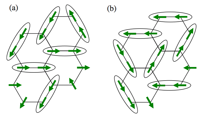
Figure 33: Some of the pseudo spin configurations where the honeycomb lattice is covered by NN bonds with the minimum bond energy. One of the q=1 states in (a) and one of the q=-1 in (b). In NN bonds surrounded by ellipses, the bond energy is the lowest Nasu et al. (2008).

The numerical value of the spectral gap between the ground state and the next excited state was found to progressively diminish as the system size was increased Nasu et al. (2008). Currently, it is not clear if this reflects the existence of gapless modes or point to a degeneracy of the system. Generally, in many spin (and pseudo-spin) systems, similar results appear in simpler systems that harbor bona fide SU(2) symmetries where the Lieb-Schultz-Mattis theorem and more recent extensions exist Lieb et al. (1961); Hastings (2004). It was furthermore found that the ground states might be approximated by an ansatz wavefunction of the type Nasu et al. (2008)

$$|\Psi^{(\pm)}\rangle={\cal{N}}\sum_{l}{\cal{A}}_{l}\{|\psi_{l}^{(\uparrow)}\rangle\pm|\psi_{l}^{(\downarrow)}\rangle\}.$$ (183)

In Eq. (183), ${\cal{N}}$ is a normalization constant, $\{{\cal{A}}_{l}\}$ are variational parameters and the states $|\psi_{l}^{(\uparrow,\downarrow)}\rangle$ schematically represented in Fig. 33 are somewhat akin to the classical configurations discussed in panel (a) of Fig. 29.

Explicitly,

$$|\psi^{(\uparrow)}_{l}\rangle=\prod_{\langle ij\rangle_{l}}U(\phi_{\gamma})|\uparrow\uparrow...\uparrow\rangle.$$ (184)

In the above, $l$ denotes a set of links $\langle ij\rangle$ for which the fully polarized state $|\uparrow...\uparrow\rangle$ will be rotated so that the pseudo-spins will be parallel to the links in the set $l$. In Eq. (184) we will, specifically, set for a single pair of sites $i$ and $j$ on the link $\langle ij\rangle$Nasu et al. (2008)

$$U(\phi_{\gamma})_{\langle ij\rangle}=\exp[-i\phi_{\gamma}(T_{i}^{y}+T_{j}^{y})]$$ (185)

where $\gamma$ is set by the spatial direction of the link between $i$ and $j$: $(\phi_{1},\phi_{2},\phi_{3})=(0,2\pi/3,4\pi/3)$. Thus, the states of Eq. (183) correspond to a linear superposition of “dimer states” , e.g.,Nogueira & Nussinov (2009); Kivelson et al. (1987); Rokshar & Kivelson (1998); Nussinov et al. (2007). In this case, the dimer states $|\psi^{\uparrow(\downarrow)}_{l}\rangle$ correspond to states wherein the pseudospins are parallel (or antiparallel) to the spatial direction. Kinetic tunneling between different dimer states can lower the energy of such states, see Fig. 34.

Thus, in the space spanned by the dimer states $\{|\psi^{(\uparrow/\downarrow)}_{l}\rangle\}$ certain admixtures of these states (with certain sets of the amplitudes $\{{\cal{A}}_{l}\}$ in Eq. (183) can be selected by quantum fluctuations.

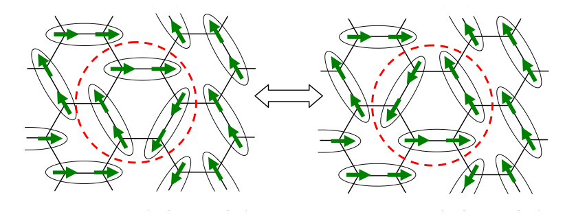
Figure 34: One example for the two pseudospin configurations where a resonance state is possible due to the off-diagonal matrix element Nasu et al. (2008).

IX.6 Checkerboard Lattice Compass Models

The most prominent compass models have been inspired by orbital or other interactions on cubic or other geometrically unfrustrated lattices. We have briefly touched on some aspects of geometric frustration in different arenas in sections (V.4,V.3.6) and elsewhere. We now explicitly turn to compass models on the checkerboard lattice. In subsection III.3.2 [and in particular in Eq. (47)], we briefly introduced the checkerboard on the checkerboard lattice Nasu & Ishihara (2011b),Nasu et al. (2012b). The checkerboard lattice, a two dimensional rendition of the pyrcholore lattice, is a prototypical frustrated lattice. The system of Eq. (47) was motivated by examining, within second order perturbation theory (assuming the kinetic term is small relative to the Coulomb penalty), a spinless Hubbard model on this lattice. This model exhibits $d=1$ symmetries in the form Nasu et al. (2012b) of

$$O_{l}=\prod_{i\in l}\tau^{z}_{i},$$ (186)

where $l$ denote diagonals that run across the system either in the $\langle 11\rangle$ or $\langle 1\overline{1}\rangle$ directions. By the generalization of Elitzur’s theorem Batista & Nussinov (2005); Nussinov et al. (2012b), these symmetries cannot be broken at finite temperatures. Some limits of the problem are obvious. When $|J_{x}|\gg|J_{z}|$, as each site lies on only one of the two diagonal directions ($\langle 11\rangle$ or $\langle 1{\overline{1}}\rangle$), the Hamiltonian of Eq. (47) reduces to that of decoupled diagonal chains with Ising $\tau_{i}\tau_{j}$ interactions between nearest neighbors. In the other extreme limit, that of $|J_{z}|\gg|J_{x}|$, interactions along the diagonals become negligible and the system becomes a two dimensional Ising model on the square lattice with nearest neighbor $\tau_{i}^{z}\tau_{j}^{z}$ interactions. In tandem with these limits, it was reported Nasu & Ishihara (2011b); Nasu et al. (2012b) that at low temperatures, for $|J_{x}|\lesssim 2|J_{z}|$, uniform or Neel (dependent on the sign of $J_{z}$) Ising order appears. By contrast, when $2|J_{z}|\lesssim|J_{x}|$, the decoupled chain like character leads, on an $L\times L$ lattice, to a $2^{2L}$ degeneracy similar to that found for the square lattice 90^∘ compass model. In the antiferromagetic variant of this system, at zero temperature, a first order transition between the two low phases was found at $J_{x}\simeq 2.7J_{z}$. Several approaches Nasu & Ishihara (2011b); Nasu et al. (2012b) suggest that there is a finite temperature tricritical point in the vicinity of $J_{x}=2J_{z}$.

IX.7 Arbitrary Angle Compass Models

We now discuss the arbitrary angle square lattice compass models Cincio et al. (2010) of Eq. (45). The symmetry of the ground states of these systems changes character at an angle $\theta_{c}$ which is very close to the right angle value of the 90^∘ compass model. The second order transition at $\theta=\theta_{c}$ is associated with the doubling of the ground state degeneracy. Specifically, for $\theta<\theta_{c}$, the system of Eq. (45) has two degenerate ferromagnetic ground states with a spontaneous magnetization that is parallel to anti-parallel to the $\tau^{x}$ (or $\pi^{x}+\pi^{y}$) direction. Conversely when $\theta>\theta_{c}$, there are four degenerate ground states with pseudo-spins along the $\pm\pi^{x}$ or $\pm\pi^{y}$ directions. For the pseudo-spin 1/2 realization of Eq. (45), it was numerically seen that $\theta_{c}\simeq 84.8^{\circ}$. As the pseudo-spin value increases and the system becomes more classical, $\theta_{c}$ monotonically increases and veers to 90^∘ in the classical limit. Thus, the four-fold degenerate phase is promoted by quantum fluctuations.

IX.8 XXZ Honeycomb Compass Model

In section II.1.3 [in particular, in Eq. (18)] the XXZ honeycomb compass model Nussinov et al. (2012a) was introduced (see also Fig. 5). This model can be mapped onto a quantum Ising gauge theory on a square lattice Nussinov et al. (2012a)

$$H_{QIG,XXZ}=-\sum_{\bf x~{}bonds}J_{x}^{\ell}\sigma^{x}_{\ell}-\sum_{\bf y~{}bonds}J_{x}^{\ell}\sigma^{x}_{\ell}$$

$$-\sum_{\bf z~{}bonds}J_{z}^{\ell^{\prime}}\prod_{\ell\in P_{\ell^{\prime}}}\sigma_{\ell}^{z}.$$ (187)

A few explanations are in order concerning this Hamiltonian. The links $\ell$ and the associated coupling constants $J^{\ell}$ refer to the links of the original honeycomb lattice; these links can be oriented along either the $x$, $y$,or $z$ directions of the honeycomb lattice. In Eq. (IX.8), the Pauli operators $\sigma_{\ell}^{x,z}$ are located at the centers $\ell$ of the square lattice which is formed by shrinking all of the vertical (or z-) links of the honeycomb lattice to individual point. After such an operation, the resulting (topologically square) lattice is comprised of x- and y- type links. As seen in Eq. (IX.8), there is a field $h=J_{x}$ that couples to the Pauli x operator on each such link. This is augmented by a plaquette term (the last term in Eq. (IX.8)). The plaquette $P_{\ell}^{\prime}$ is formed by the centers of the four links (two x-type links and two y-type links) that are nearest neighbors to the center of a vertical z-type link $\ell$. The product $\prod_{\ell\in P_{\ell^{\prime}}}\sigma_{\ell}^{z}$ denotes the product of all four $\sigma^{z}$ operators at the centers of links of the square plaquette that surrounds an original vertical link $\ell$ that has been shrunk to a point. The sum over the original vertical links (z-bonds) becomes, in Eq. (IX.8), a sum over all plaquettes of a square lattice formed the shrinking of all vertical links. The link center-points of this square lattice coincide with those formed by the center-points of the x- and y-type bonds of the original honeycomb lattice. When all of the coupling constants $J_{x,z}^{\ell}$ are isotropic, the system is that of the canonical uniform standard transverse field Ising gauge theory which, as is well known, maps onto the 3D Ising gauge theory. The 3D Ising gauge theory is dual to the standard 3D Ising model on the cubic lattice Wegner (1971); Kogut (1979). Thus, the uniform XXZ honeycomb compass model is dual to the 3D Ising model and exhibits a finite temperature phase transition with the standard 3D Ising exponents Nussinov et al. (2012a). As is evident in Eq. (IX.8), not all coupling constants $J_{x,z}^{\ell}$ need to be of the same strength. As the disordered transverse field Ising gauge theory can exhibit a spin-glass type transition, the XXZ honeycomb model may also correspond to a spin glass when it is non-uniform Nussinov et al. (2012a). Additional information concerning the quantum Ising gauge theory appears in section IX.11.

IX.9 Plaquette Orbital Model

The authors of Biskup & Kotecky (2010) studied the classical realization of the “plaquette orbital model” Wenzel & Janke (2009) and certain quantum variants. Below, these results are reviewed.

IX.9.1 Exact Symmetries

Examining the Hamiltonian of Eq. (46) and Figure 8, we note that the inversion of the four pseudo-spins $\tau^{x}_{i}\to-\tau^{x}_{i}$ on an A plaquette (while leaving $\tau^{y}_{i}$ unchanged) constitutes a local symmetry. A similar effect occurs with $x$ and $y$ interchanged on any of the B-type plaquettes. These local (i.e., gauge) symmetries are recast in terms of the following 4-site symmetry operators of the $T=1/2$ quantum Hamiltonian of Eq. (46) ($[U_{\Box_{{\cal{A}}}},H]=[U_{\Box_{{\cal{B}}}},H]=0$),

$$U_{\Box_{{\cal{A}}}}=\prod_{i\in\Box_{{\cal{A}}}}\tau^{y}_{i},~{}~{}U_{\Box_{{\cal{B}}}}=\prod_{j\in{\Box_{{\cal{B}}}}}\tau^{x}_{j}.$$ (188)

In Eq. (188), ${\cal{A}}$ denotes any plaquette of the A type and, similarly, ${\cal{B}}$ denotes any plaquette of the B type. By Elitzur’s theorem, at any finite temperature ($T>0$), all expectation values must be invariant under the symmetries of Eq.(188).

IX.9.2 Classical Ground States & Emergent Symmetries

By rewriting, similar to the analysis for the classical 120 and 90 degree models, Nussinov et al. (2004); Biskup et al. (2005), the Hamiltonian of Eq.(46) as a sum of squares and using uniform states as classical “variational states”, Biskup & Kotecky (2010) demonstrated that all classical ground states of Eq. (46) are uniform states up to the application of the classical version of the local symmetries of Eqs.(188). In particular, for $J_{A}>J_{B}$, a state which is fully polarized along the $x$ axis constitutes a ground state; this state can be further mutated by the local inversion gauge transformations. Similar to the situation in the classical 120 degree and compass models a continuous symmetry emerges in the classical ground state sector. When $J_{A}=J_{B}$, any constant uniform state of the pseudo-spins ${\bm{T}}_{\bm{r}}$ is a ground state of the classical system. As these classical vectors can point anywhere on the unit disk, a continuous rotational symmetry appears.

IX.9.3 Finite Temperature Order out of Disorder

Similar to the situation in the classical 120 degree and 90 degree compass models, a finite temperature order out of disorder mechanism lifts the ground state degeneracy Nussinov et al. (2004); Biskup et al. (2005); Mishra et al. (2004), and leads, at low positive temperatures ($0<T<T_{0}$) to a nematic type order in the plaquette compass model wherein most of the configurations have a majority of the pseudo-spins aligned along either the $(\pm{\bm{e}}_{x})$ or the $(\pm{\bm{e}}_{z})$ directions Biskup & Kotecky (2010). Due to the (classical version of the) local symmetries of Eqs. (188), both sign of the orientation ($\pm$) are equally likely.

Following Biskup et al. (2007), low temperature order was also proven to hold in the quantum model when the magnitude of the pseudo-spin is sufficiently large ($|{\bm{T}}|>c\beta^{2}$ with $c$ a positive constant and $\beta$ the inverse temperature) Biskup & Kotecky (2010). The technical reason for requiring a sufficiently large pseudo-spin is that within the proof of Biskup & Kotecky (2010); Biskup et al. (2007), thermal fluctuations were assumed to dominate of quantum fluctuations.

IX.10 Gell-mann Matrix Compass Models

The two Gell-mann matrix compass models of Eqs. (122, 123), derived from Eq. (121), have very interesting and distinct behaviors Chern & Wu (2011).

IX.10.1 Cubic Lattice Gell-mann Matrix Compass Model

As the two Gell-mann matrices $\lambda^{(3)}$ and $\lambda^{(8)}$ are diagonal and commute with one another, the quantum model of Eq. (122) is essentially classical Chern & Wu (2011).

$T=0$:
The ground state energy per site $E/N=-2J/3$ is consistent with 2/3 of the bonds being minimized and the remaining 1/3 being frustrated. The two-point correlation function $\langle{\bm{\lambda}}_{i}\cdot{\bm{\lambda}}_{j}\rangle$ exhibits rapidly decaying oscillations and is essentially vanishing for distances $|{\bm{r}}_{ij}|\geq 5$ lattice constants Chern & Wu (2011).

$T>0$:
Monte Carlo simulations were performed. An integration from the specific heat curve indicates that there is a large residual entropy at zero temperature. Although not explicit estimate was given in Chern & Wu (2011) for viable transitions, judging from the data shown the sharp specific heat peak occurs at a temperature $T\sim 0.7J$.

IX.10.2 Diamond Lattice Gell-mann Matrix Compass Model

For a single pair of nearest neighbor sites on the lattice along the ${\bm{n}}_{0}$ direction ($i$ and $j$), the minimum of the corresponding term in Eq. (123) is achieved when the corresponding orbital states are $3^{-1/2}(|p_{x}\rangle+|p_{y}\rangle+|p_{z}\rangle)$ and $2^{-1/2}(|p_{x}\rangle-|p_{y}\rangle)$. Similar to the case of the Gell-mann model on the cubic lattice and, more generally, compass models, the system is frustrated and not all interactions can be simultaneously minimized. As shown in Chern & Wu (2011), the ground states are of the form $|\psi\rangle=\prod_{i}|\lambda_{i}$ with for any site $i$, the local state $|{\bm{\lambda_{i}}}\rangle=|\pm{\bm{e}}_{x}\rangle,|\pm{\bm{e}}_{y}\rangle$ or $|\pm{\bm{e}}_{z}\rangle$ such that for all nearest neighbor pairs $\langle ij\rangle$,

$$({\bm{\lambda}}_{i}\cdot{\bm{e}}_{ij})({\bm{\lambda}}_{j}\cdot{\bm{e}}_{ij})=-\frac{1}{3}.$$ (189)

When expressed in terms of the original orbital degrees of freedom, the local states are, explicitly, $|\pm{\bm{e}}_{x}\rangle=2^{-1/2}(|p_{y}\rangle\pm|p_{z}\rangle)$ and cyclic permutations thereof (i.e., $|\pm{\bm{e}}_{y}\rangle=2^{-1/2}(|p_{z}\rangle\pm|p_{x}\rangle)$ and $|\pm{\bm{e}}_{z}\rangle=2^{-1/2}(|p_{x}\rangle\pm|p_{y}\rangle)$).

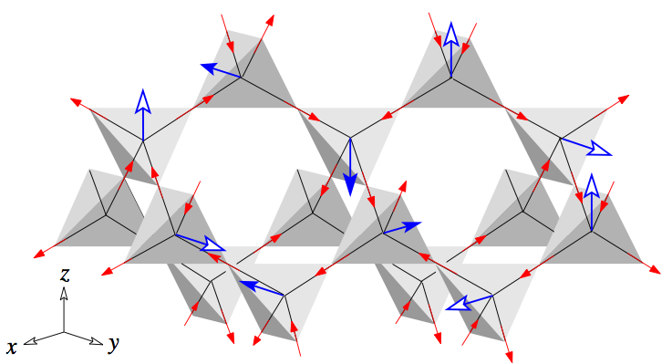
Figure 35: A configuration of the pseudo-vectors on the diamond lattice and its mapping to the spin-ice state on the dual pyrochlore lattice. The pseudo-vector only assumes six different values $\langle\mu i\rangle=\pm\hat{x},\pm\hat{y},\pm\hat{z}$ in the ground states, corresponding to ($p_{y}\pm p_{z}$), ($p_{z}\pm p_{x}$), and ($p_{x}\pm p_{y}$) orbitals, respectively. These six orbital configurations are mapped to the six 2-in-2-out ice state on a tetrahedron. Chern & Wu (2011).

As shown in Fig. (35), the states $|\pm{e}_{x,y,z}\rangle$ at any site $i$ can be represented by corresponding red arrows on the pyrochlore lattice formed by the centers of all nearest neighbor links $\langle ij\rangle$. Specifically, these arrows are given by

$${\bm{R}}_{\langle ij\rangle}=\sigma_{i}^{\gamma}{\bm{e}}_{ij}(=-\sigma_{j}^{\gamma}{\bm{e}}_{ij}),$$ (190)

where, with ${\bm{e}}_{ij}$ denoting a unit vector from site $i$ to site $j$, the Ising type variables $\sigma_{i}^{\gamma}=\pm 1$ are given by $\sigma_{i}^{\gamma}=\sqrt{3}({\bm{\lambda}}_{i}\cdot{\bm{e}}_{ij})$. Following Chern & Wu (2011), we next focus on the basic tetrahedrons of pyrochlore lattice (that have the vertices of the original diamond lattice at their centers). As a result of the condition of Eq. (189), there are two incoming and two outgoing arrows ${\bm{R}}$ towards the center of each tetrahedron. This is the so-called “ice condition” which appears in many other systems and leads to an extensive degeneracy Lieb (1967); Nagle (1966) which according to the Pauling estimate would be $S\approx Nk_{B}\ln(3/2)\simeq 0.405Nk_{B}$ Chern & Wu (2011). (Note that according to the more accurate estimate of Nagle Nagle (1966) this would be $S\approx 0.4102Nk_{B}$). Similar to the Gell-mann matrix model on the cubic lattice, two-point correlations within the ground state are decaying. In general, the correlations associated with extensively degenerate ice states are dipolar type power law correlations $\langle{\bm{\lambda}}_{i}\cdot{\bm{\lambda}}_{j}\rangle\sim|{\bm{r}}_{ij}|^{-3}$. Villain (1972); Stillinger & Cotter (1973); Youngblood & Axe (1981); Ioffe & Larkin (1989); Huse et al. (2003); Henley (2005); Nussinov et al. (2007). Such correlations were indeed numerically verified by Chern and Wu in their system Chern & Wu (2011). The ice condition and its breaking are known to lead to effective fractional charges and related effects as found in different contexts Fulde et al. (2002); Nussinov et al. (2007); Castelnovo et al. (2008); Powell (2011); Chang et al. (2012). In particular, when the temperature $T>0$, thermal excitations out of the ground state ice condition manifold can lead to deconfined fractional charges (with dipolar correlations). It would be interesting to see what is the corresponding physics in this orbital system.

IX.11 Symmetric Extended Compass Hubbard Models

In section V.1.5, and in Eq. (101) in particular, a compass type Hubbard model was introduced that, aside from lattice hopping terms, further included electronic pair creation and annihilation terms. Both of these terms (kinetic and pairing) were of the compass type. In Eq. (101), the spatial indices of the electronic creation and annihilation operators involved were determined by the spin polarization. The particular, symmetric, variant written of the extended compass Hubbard model, that of Eq. (101), in which the pairing and hopping amplitudes are of equal strength, is amenable to an exact result. It can be demonstrated Nussinov et al. (2012a) that the square lattice system of Eq. (101) is dual to the quantum Ising gauge theory (QIG) on the dual lattice. This dual lattice (which is also a square lattice) is formed by regarding each site $i$ of the original square lattice as the center of a minimal square (or plaquette) of the dual lattice. The QIG theory was already written down as its associated couplings pertain to the XXZ honeycomb compass in Eq. (IX.8). We now do so anew for the symmetric extended compass Hubbard model. The Hamiltonian of the quantum Ising gauge theory which is dual to the theory of Eq. (101) is given by

$$H_{QIG,SEHCM}=-2\sum_{l}t_{l}\sigma^{x}_{l}-\sum_{P}U_{i}\prod_{l\in P_{i}}\sigma^{z}_{l}.$$ (191)

The index $l$ in Eq. (191) denotes a link of the square lattice. In reference to the symmetric extended compass Hubbard model of Eq. (101), $t_{l}$ is the hopping amplitude between two sites in the original electronic system. In the spin Hamiltonian of Eq. (191), a Pauli operator is placed at the center of each link $l$ of the square lattice. The first term in Eq. (191), thus physically corresponds, at each such link $l$, to a magnetic field term along the $x$ direction which is of strength $t_{l}$. The second term in Eq. (191) is the standard “plaquette” term of classical gauge theories. $P_{i}$ denotes any elementary plaquette of the square lattice on which Eq. (191) is defined (corresponding to a site $i$ on the original square lattice model of Eq. (101)). $\prod_{l\in P_{i}}\sigma^{z}_{l}$ is the product of the four $\sigma^{z}$ operators on the links $l$ of such a minimal square plaquette $P_{i}$ of the lattice. In the absence of the first (magnetic field) term in Eq. (191), the Hamiltonian is that of the classical square lattice Ising gauge theory Kogut (1979) (which is trivially dual to an Ising chain). The field $t_{l}$ along the transverse $x$ direction leads to quantum fluctuations between different classical spin states. These fluctuations are the origin of the name “quantum Ising gauge theory”. As is well known, the square lattice quantum Ising gauge theory can be mapped onto the 3D classical Ising gauge theory (the theory given solely by square plaquettes terms on the cubic lattice). The 3D Ising gauge theory is, in turn, dual to the standard Ising model on the cubic lattice. Thus, similar to the discussion in section IX.8, by the equivalence between the theories of Eqs.(101, 191) one can adduce much information. These considerations and make specific remarks about (i) the spatially uniform and (ii) disordered realizations of this theory.

The spatially uniform system When all of the pairing/hopping amplitudes $t_{l}$ and the Hubbard energy terms $U_{i}$ in Eq. (101) are spatially uniform and equal to fixed values $t$ and $U$, the system is equivalent to and exhibits canonical 3D Ising behavior. At zero temperature, a 3D Ising critical transition appears at a ratio of

$$\Big{(}\frac{t}{U}\Big{)}_{crit}=0.14556.$$ (192)

Disordered systems The mapping Nussinov et al. (2012a) between the symmetric extended compass Hubbard model of Eq. (101) and the quantum Ising gauge theory of Eq. (191) is general applies to any set of couplings $\{t_{l},U_{i}\}$. As is well known, sufficiently disordered Ising models (in which couplings are non-uniform) may display a spin glass type behavior. Thus, by the correspondence between Eqs. (101, 191), the electronic system given by random symmetric extended compass Hubbard model may display spin glass behavior.

IX.12 Heisenberg-Kitaev Models & Honeycomb Iridates

In section V.1.8, we reviewed how spin-orbit effects may lead to the Heisenberg-Kitaev model of Eq. (113). We will now review various results obtained on the model.

IX.12.1 Phase Diagram of Heisenberg-Kitaev Model

The overall multiplicative constant $C$ in Eq. (113) can be absorbed by scaling the temperature $T\to T/C$. As a function of $\alpha$, the Heisenberg-Kitaev model has a wealth of phases. Recent experiments Singh & Gegenwart (2010); Liu et al. (2011); Singh et al. (2012); Choi et al. (2012) seem to agree with theoretical analysis Chaloupka et al. (2010); Reuther et al. (2011); Jackeli & Khaliullin (2009); Jiang et al. (2011); Chaloupka et al. (2013). These notably include the viable presence of a zigzag phase and its associated magnetic susceptibility and spin-wave spectra. We remark that some phases similar to those that are found in the Heisenberg-Kitaev model appear in certain frustrated U(1) symmetric XY models on the honeycomb lattice Varney et al. (2011). Below we first examine specific properties of the Heisenberg-Kitaev model.

Exact self-duality of the Heisenberg-Kitaev model:
Although not explicitly stated earlier in these terms, the Heisenberg-Kitaev model of Eq. (113) exhibits an elegant and exact self-duality- i.e., a self-duality which exactly applies to the entire energy spectrum of the theory (not only that which emerges at low energies (or other sectors) as in many, far weaker, emergent self-dualities). This exact self-duality is made explicit via a unitary transformation (a sublattice dependent canonical 180^∘ rotation) that maps the Hamiltonian of Eq. (113) back to itself yet with rescaled couplings Chaloupka et al. (2010); Khaliullin (2005b); Chaloupka et al. (2013). Before explicitly reviewing this transformation, one rewrites Eq. (113). The first (Heisenberg type) term in Eq.(113) contains also a (Kitaev type) contribution of the form of $\tau^{\gamma}_{i}\tau^{\gamma}_{j}$ but with a sign that is opposite to the first. As throughout this review, we denote by ${\bf{e}}_{x,y,z}$ the three unit vector directions on the honeycomb lattice. Specifically, we define these to point vertically up (${\bf{e}}_{z}$) or downwards while veering to the right or left (${\bf{e}}_{x,y}$). With $i\in A$ denoting lattice sites that belong to the even sublattice of the honeycomb lattice (i.e., all lattice sites that lie at the bottom of all vertical links of the lattice), the Hamiltonian of Eq. (113) reads

$$H_{HK}=C\sum_{i\in A}\sum_{\gamma=x,y,z}\Big{[}(1-3\alpha)\tau^{\gamma}_{i}\tau^{\gamma}_{i+{\bf{e}}_{\gamma}}$$

$$+(1-\alpha)\sum_{\gamma^{\prime}\neq\gamma}\tau^{\gamma^{\prime}}_{i}\tau^{\gamma^{\prime}}_{i+{\bf{e}}_{\gamma^{\prime}}}\Big{]}.$$ (193)

In the second line of Eq. (193), the sum is performed over all honeycomb lattice directions $\gamma^{\prime}=x,y$ or $z$ that differ from a given $\gamma$. A spatially dependent rotation Khaliullin (2005b); Chaloupka et al. (2010) can simplify this problem. Specifically, the system is partitioned into four sublattices [see Fig. 36] and then a site dependent rotation operator is applied,

$${\bm{\tau}}_{i}\to{\bm{\tilde{\tau}}}_{i}=U^{\dagger}_{i}{\bm{\tau}}U_{i}.$$ (194)

The site dependent unitary operator $U_{i}$ may, depending to which sublattice the site $i$ belongs to (see Fig. (36), rotate on three of the sublattices the iso-spin vector ${\bm{\tau}}_{i}$ by 180 degrees about one of three associated ($x$, $y$, or $z$) iso-spin directions while acting as the identity operator [${\bm{\tau}}_{i}={\bm{\tilde{\tau}}}_{i}$] for sites $i$ that belong to the fourth sublattice. As in other general cases, this self-duality implies that couplngs related to one another by the self-duality lead to identical thermodynamics and dynamics.

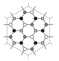
Figure 36: The supercell of the four- sublattice system enabling the transformation of the model  Chaloupka et al. (2010).

In the rotated basis, the Hamiltonian of Eq. (113) reads

$$\tilde{H}_{HK}=C\sum_{\langle ij\rangle||\gamma}[(\alpha-1){\bf{\tilde{{\tau}}}}_{i}\cdot{\bf{\tilde{{\tau}}}}_{j}+(2-4\alpha){\tilde{\tau}}_{i}^{\gamma}{\tilde{\tau}}_{j}^{\gamma}].$$ (195)

That is, the unitary transformation maps the Hamiltonian back to itself yet with new parameters; as such, this sublattice dependent site dependent rotation operation realizes a self-duality transformation. Written in terms of the original parameters in Eq. (193), one sees that Eq. (195) implies a transformation

$$\alpha\to(2\alpha-1)/(3\alpha-2),$$

$$C\to C(3\alpha-2).$$ (196)

Alternatively, under this self-duality transformation, in the top line of Eq. (113), $J_{1}\to(J_{1}-2J_{2})$ while $J_{2}\to-J_{2}$. In the $(A,\varphi)$ parameterization of Eq. (113), $\tan\varphi\to(-\tan\varphi-1)$ Chaloupka et al. (2013) and $A\to A\sqrt{(2+2\tan\varphi+\tan^{2}\varphi)/(1+\tan^{2}\varphi)}$. As in all self-dualities, a repeated application of the transformation twice restores the original coupling constants (as is evident in this case from a repeated application of the sublattice dependent 180^∘ rotations). A schematic of the self-duality in this parameterization and the associated phases and transitions which will shortly be elaborated on later is provided in Fig. (21). Fig. 37 reproduced from Chaloupka et al. (2013) further provides a schematic of the types of ground states found for different values of $\varphi$; ground states related to each other by the self-duality transformation can be formed from one another by applying the sublattice dependent 180^∘ rotation discussed above. We next turn to particular values of the parameters for which an exact characterization of the system or ground states is possible.

Figure 37: (a) Phase diagram of the Kitaev-Heisenberg model containing 2 spin-liquid and 4 spin-ordered phases. The transition points (open dots on the $\phi$ circle) are obtained by an exact diagonalization. The gray lines inside the circle connect the points related by the exact mapping (see text). Open and solid circles in the insets indicate up and down spins. The rectangular box in the zigzag pattern (top-left) shows the magnetic unit cell. (b) Ground-state energy and its second derivative revealing the phase transitions Chaloupka et al. (2013).

Exact orders of the quantum Heisenberg-Kitaev model at special points:
The quantum system of Eq. (113) can be illustrated to exactly harbor six disparate types of low temperature orders Chaloupka et al. (2010); Khaliullin (2005b); Chaloupka et al. (2013); Reuther et al. (2011); Schaffer et al. (2012) at different couplings. Each of the points below lies within a phase that extends over a finite range of parameters. Earlier works focused on three of the phases present for $C>0$ and $0\leq\alpha\leq 1$ (or, equivalently, those in the fourth quadrant, $-\pi/2\leq\varphi\leq 0$). The full totality of the six phases discussed below was first enumerated in Chaloupka et al. (2013). The full spectrum of phases and their transitions are evident in Fig. (21); the lower panel in this figure provides the results of exact diagonalization. Further numerical results will be reviewed later on. The character of the transitions (whether continuous or discontinuous) between any two given phases must be of the same type as that between the two other phases to which these given phases are dual to. In the discussion below, we further invoke the self-duality of the Heisenberg-Kitaev model to illustrate that one may consistently infer exact statements about the system and its low temperature orders.

(i). $\alpha=0$ and $C>0$ (or, equivalently, $\varphi=0$):
Heisenberg antiferromagnet
At this point, the model of Eq. (113) reduces to the Heisenberg antiferromagnetic model ($J_{1}=0,J_{2}>0$) on the honeycomb lattice exhibiting global SU(2) rotational invariance. This Heisenberg model on the honeycomb lattice Oitmaa & Betts (1978); Reger et al. (1989); Oitmaa et al. (1992); Mattsson et al. (1994); Fouet et al. (2001) exhibits Neel order yet with a notably reduced magnetization as a consequence of quantum fluctuations. As a symmetry analysis shows Jiang et al. (2011), the system is six-fold degenerate.

(ii). $\alpha=1$ and $C>0$ (or $\varphi=-\pi/2$):
Ferromagnetic Kitaev model
Here, Eq. (113) reduces to the ferromagnetic variant of Kitaev’s honeycomb model Kitaev (2006). The system exhibits no broken symmetries and a wealth of fascinating characteristics Kitaev (2006). All two point spin correlations vanish for distances beyond one lattice constant Baskaran et al. (2007); Chen & Nussinov (2008).

(iii). $\alpha=0$ and $C<0$ (or $\varphi=\pi$):
Heisenberg ferromagnet
When $J_{2}<0$ and $J_{1}=0$, the Heisenberg-Kitaev model of Eq. (113) becomes that of an SU(2) invariant ferromagnetic system. At these parameters, the system is dual to the $\alpha=1/2$ and $C>0$ case discussed above.

(iv). $\alpha=1$ and $C<0$:
Antiferromagnetic Kitaev model
When $J_{1}<0$ and $J_{2}=0$ (or, equivalently, $\phi=\pi/2$), the model reduces to the antiferromagnetic variant of Kitaev’s honeycomb model. At this point, the system is, by another duality transformation (as may, e.g., be seen by the “bond algebraic” technique to be reviewed and applied to the Kitaev model in subsection X.3) trivially dual to that of the ferromagnetic model. As such, here the system is a spin liquid. However, by contrast to the ferromagnetic Kitaev model, the system is less stable to Heisenberg type perturbations which more readily alter it and promote various orders.

(v). $\alpha=1/2$ and $C>0$ (or $\varphi=-\pi/4$):
Fluctuation free quantum stripe antiferromagnet
At this point the system is exactly solvable due an elegant consideration of Chaloupka et al. (2010).

When $\alpha=1/2$ (or , equivalently, $J_{1}=2J_{2}$ or when $\tan\varphi=-1$), this spatially dependent spin rotation of Eq. (194) maps this system to a ferromagnetic Heisenberg model, i.e., to the Hamiltonian

$$\tilde{H}_{HK,~{}\alpha=1/2}=-\frac{1}{2}\sum_{\langle ij\rangle}{\bm{\tilde{\tau}}}_{i}\cdot{\bm{\tilde{\tau}}}_{j}.$$ (197)

Thus, when $\alpha=1/2$, the system harbors the continuous global SU(2) symmetry of the ferromagnet.

Moreover, when $\alpha=1/2$, the ground states of the full quantum problem of Eqs.(113,193) are thus uniform ferromagnetic states Chaloupka et al. (2010) in the rotated basis ${\bm{\tilde{\tau}}}$. Applying the inverse transformation, ${\bm{\tilde{\tau}}}\to{\bm{\tau}}$, a uniform ferromagnetic state in the ${\bm{\tilde{\tau}}}$ basis is seen to correspond to a stripe-like antiferromagnet in the original ${\bm{\tau}}$ basis. A cartoon is shown in Fig. 38.

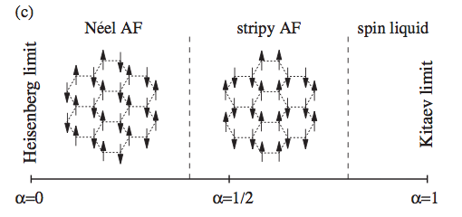
Figure 38: Schematic phase diagram for $C>0$ in Eq. (113): With increasing $\alpha$, the ground state changes from the Neèl AF order to the stripy AF state (being a fluctuation-free exact solution at $\alpha=1/2$) and to the Kitaev spin liquid. See the text for the critical values of $\alpha$. Chaloupka et al. (2010).

Chaloupka et al., 2010 noted that this stripy antiferromagnet state is an exact eigenstate at $\alpha=1/2$ and is thus fluctuation free. When $\alpha\neq 1/2$, symmetry considerations indicate that a six-fold degeneracy persists over the entire extent of the stripy ferromagnetic state Jiang et al. (2011).

(vi): $\alpha=1/2$ and $C<0$ (or $\varphi=3\pi/4$):
Zig-zag phase
This point with, in the original Hamiltonian of Eq. (113), $J_{1}=2J_{2}>0$ is dual to the point at $\varphi=0$ ($\alpha=1/2,~{}C>0$) discussed above. Thus, the ($\varphi=0$) antiferromagnetic states on the honeycomb model become transformed by the sublattice dependent 180^∘ rotation that realizes the self-duality transformation into those present when $\varphi=3\pi/4$. As antiferromagnetic Neel order (such that for $\varphi=0$) is transformed, via this sublattice dependent rotation, into a “zig-zag” order (i.e., one with ferromagnetic zigzag chains of the pseudo-spins which are antiferromagnetically coupled to each other), it follows that when $\varphi=3\pi/4$, the system may exhibit such zig-zag ordering. As the zig-zag state is, at this point, an exact (stationary) eigenstate of the Hamiltonian, this eigenstate is, similarly to the $\alpha=1/2$ and $C>0$ point above, also fluctuation free. As such, associated with spin-wave fluctuations, gapless spin-wave modes (i.e., Goldstone modes) appear at this point. Such zig-zag ordering is of possible pertinence as several experiments have reported observations consistent with precisely such a zig-zag ordering Liu et al. (2011); Choi et al. (2012); Singh & Gegenwart (2010); Singh et al. (2012).

IX.12.2 Spin waves and Exact Transition Points

Similar to the results reviewed for the 120^∘ compass model in Section VIII.2, a spin-wave type analysis may be performed about, for instance, a zig-zag type ground state. The bare spin-wave dispersion for such fluctuations was reported in Chaloupka et al. (2013). Employing an $(a\times b)=(\sqrt{3}a_{0}\times a_{0})$ rectangular unit cell similar to that in Choi et al. (2012) where $a_{0}$ is the length of the hexagon.Writing the reciprocal lattice vector as ${\bf{k}}=(\frac{2\pi}{a}h,\frac{2\pi}{b}k)$, the resulting four dispersive branches may be exactly computed Chaloupka et al. (2013).

For a choice of parameters $(J_{1},J_{2})=-(20.9,4.01)$ in Eq. (113) [or, equivalently, $\alpha=0.723$, $C=-14.46meV$ (corresponding to an angular parameterization with $\varphi$ in the second quadrant with $\tan\varphi\simeq 2.61$)]; these are parameters estimated for Na₂IrO₃ where there are experimental indications of a viable zig-zag phase Liu et al. (2011); Choi et al. (2012); Singh & Gegenwart (2010); Singh et al. (2012). At the solvable fluctuation free $alpha=1/2$ and $C<0$ point (or, equivalently, $\varphi=3\pi/4$) where an exact zig-zag state may be proven as discussed above, the four spin-wave mode become two pairs of degenerate modes. The lower energy set of these modes realizes the Goldstone mode behavior. For parameter values away from this point a magnon gap is expected by quantum fluctuations Chaloupka et al. (2013).

Below it is illustrated that, in a somewhat similar vein, exact statements can be made concerning transitions between classical orders in this system.

(i) $\alpha=1/3$ and $C>0$ (or $\varphi=\tan^{-1}(-1/2)\simeq-26.563^{\circ}$): Transition between the Neel and stripe antiferromagnetic ground states. This point has been examined earlier Chaloupka et al. (2010). Examining Eq.(193), one sees that associated with each nearest neighbor link of the lattice along the $\gamma=x,y$ or $z$ direction only the exchange interactions amongst two components of the pseudo-spin $\gamma^{\prime}\neq\gamma$ appear. That is, e.g., associated with a link along the $\gamma=x$ direction, one explicitly has

$$H_{HK;~{}(i,i+{\bf{e}}_{x})}=\frac{2}{3}(\tau^{y}_{i}\tau^{y}_{i+{\bf{e}}_{y}}+\tau^{z}_{i}\tau^{z}_{i+{\bf{e}}_{z}}).$$ (198)

The appearance of only two spin components suggests that symmetries may appear. Unlike the situation for $\alpha=0,1/2$ (or, equivalently, $\varphi=-\pi/4,-\pi/2$), however, these are only emergent symmetries within the ground state (i.e., zero temperature) sector of the classical model. Specifically, Ising type $d=1$ gauge like symmetries are present (corresponding to a flip of all spins along chains) and these lead to an infinite degeneracy of the ground state sector. When acting on a classical Neel ground state, such $d=1$ Ising type operations lead to the stripy antiferromagnet state. Thus, classically, the boundary between the Neel and stripy antiferromagnet ground states lies, exactly, at $\alpha=1/3$.

(ii) $\alpha=1/3$ and $C<0$: Transition between the ferromagnetic and zigzag ground states This point has not been examined in earlier works. We wish to note that the system at this point ($\alpha=1/3$ and $C<0$) is dual to that at $\alpha=1/3$ and $C>0$ (and for these values of the parameters related to it in the angular parameterization via the transformation $\varphi\to(\pi-\varphi)$). As can be established by incorporating the sublattice dependent rotation, similar to its dual point at positive $C$, the $(\alpha=1/3,C<0)$ point lies at the boundary between classical ferromagnetic and classical zigzag order.

The two semi-classical points above $(\alpha=1,C>0$) and $(\alpha=-1,C<0$) are self-dual (i.e., map onto themselves) under the self-duality transformation. Similar to its counterpart at positive $C$, the $\alpha=1$ system at negative $C$ is a spin liquid Chaloupka et al. (2013). Both systems at these points correspond to Kitaev model for ferromagnetic ($C>0$) or antiferromagnetic ($C<0$) couplings respectively. Although the ferromagnetic and antiferromagnetic Kitaev models are identical to each other and share an identical spectrum, as stated above,when Heisenberg type perturbations are introduced it is seen the ferromagnetic spin liquid is more stable and extends over a far larger range of $\varphi$ values than its antiferromagnetic counterpart Chaloupka et al. (2013). This is readily seen in Fig. 37. Related phases (including a spiral phase) may appear in the model of Eq. (115) Kargarian et al. (2012).

IX.12.3 Order by disorder

Order by disorder occurs at two different situations. One encounters:

(i) Global rotational symmetry As discussed above, when $\alpha=0,1/2$ (for both signs of the constant $C$ in Eq. (113)) the system rigorously exhibits a global SU(2) symmetry. This symmetry appears as either as a standard global uniform rotational symmetry in the case of the ferromagnet ($C<0$) or antiferromagnetic ($C>0$) Heisenberg model when $\alpha=0$ or to such a global rotational symmetry following a four sublattice dependent 180^∘ rotation in the case of the $\alpha=1/2$ to which these systems are dual. Similar to the discussion of the 120^∘ and $90^{\circ}$ compass models, within a spin-wave approximation, the classical rendition of Eq.(113) exhibits, also for $\alpha\neq 0,1/2$, an emergent continuous symmetry within its ground state sector. Similar to the situation for the 120^∘ and $90^{\circ}$ compass models, this symmetry is lifted by an order out of disorder mechanism. Physically, a spin gap opens and the system preferentially orders along one of the crystalline axes of IO₆ octahedra. The energy penalty for orienting the pseudo-spins away from the crystalline axes scales, for $\alpha$ close to 1/2, as $\Delta\simeq\frac{2}{\alpha}(\alpha-\frac{1}{2})^{2}$ Chaloupka et al. (2010).

(ii) $d=1$ Ising type symmetries Quantum fluctuations lift the above discussed emergent Ising degeneracy of the ground state sector of the classical rendition of the $\alpha=1/3$ system Chaloupka et al. (2010) and move the transition point between the two phases to a larger value of $\alpha$.

IX.12.4 Phase Transitions

There are several zero temperature transition points at values of the coupling constants that are not exactly determined.

(i) Transition between the Neel phase and the stripe antiferromagnet The boundary between the ground states of the Neel and stripy antiferromagnet ground states (a discontinuous transition by symmetry considerations) lies at $C>0$ near $\alpha\simeq 0.4$ (or $\tan\varphi\simeq-2/3$). Within second order perturbation theory Chaloupka et al. (2010), the energies of the Neel and stripy antiferromagnet states on a honeycomb lattice of $N$ sites (and $3N/2$ links) are given by

$$E_{HK,~{}Neel}\simeq-\frac{3}{16}N(3-5\alpha),$$

$$E_{HK,~{}stripy~{}AF}\simeq-\frac{1}{8}N(5\alpha-3+\frac{1}{\alpha}).$$ (199)

Setting $E_{HK,~{}Neel}=E_{HK,~{}stripy~{}AF}$ leads to $\alpha=0.4$ (and a physically irrelevant solution of $\alpha=0.2$). Numerical analysis further corroborate the existence of a first order transition between the Neel and stripy antiferromagnetic phases at $\alpha=0.4$.

(ii) Transition between the stripe antiferromagnet and the ferromagnetic Kitaev spin liquid phase In the Kitaev model (i.e., in the $\alpha=1$ limit of Eq.(113) with $C=1$), the sole nearest neighbor correlations between two spins are those associated with the iso-spin component $\gamma$ that lies along the link direction $\langle ij\rangle$ (i.e., $\gamma||\langle ij\rangle$) Baskaran et al. (2007); Chen & Nussinov (2008). An estimate employing these nearest neighbor correlation suggests that the spin liquid phase may extend beyond the Kitaev point ($\alpha=1$) up to a value of $\alpha\simeq 0.86$. This value is close to the numerically ascertained value of $\alpha\simeq 0.8$ (or $\tan\varphi\simeq-4$) for a critical point between the spin liquid and stripy antiferromagnetic phase.

Relying on the above results, in the below, additional approximate transition points are computed. The values of the transition points that one finds are consistent with those found by the exact diagonalization in Chaloupka et al. (2013).

(iii) Transition between the ferromagnetic Kitaev spin liquid and the spin ferromagnet Using the self-duality of the system one can compute the boundaries between the Kitaev spin liquid and the spin ferromagnet by relying on earlier results concerning the transition point between the stripe ferromagnet (which is dual to the stripe antiferromagnet) and the ferromagnetic Kitaev spin liquid. This approach which is now applied using the self-duality to compute the phase boundaries has not been invoked in earlier works. Setting $\alpha\simeq 0.8$ ($C>0$) to mark the transition point between the stripe antiferromagnet and the ferromagnetic Kitaev model, the self-duality illustrates that the transition between the ferromagnetic Kitaev spin liquid and the spin ferromagnet occurs at $\alpha\simeq 1.5$ and $C>0$ (or $\tan\varphi\simeq 3$ with $\varphi$ in the third quadrant). The character of the transition between the ferromagnetic Kitaev spin liquid and the ferromagnet is identical to that between the stripe antiferromagnet and the ferromagnetic Kitaev spin liquid.

(iv) Transition between the ferromagnet and the zig-zag phase Once again, one may employ the self-duality of the system to ascertain the transition point (and the character of the transition) between the ferromagnetic phase (dual to the stripe antiferromagnet) and the zig-zag phase (dual to the Neel phase). This transition occurs at $\alpha\simeq 0.25$ for $C<0$ (or, equivalently, when $\varphi$ lies in the second quadrant with $\tan\varphi=-1/3$.

IX.12.5 Overview of Numerical results

Numerical validation of the phase diagram comprised of the three phases was first obtained by Chaloupka et al. (2010). In Fig. 39, different measures are presented. Numerical results Reuther et al. (2011), Chaloupka et al. (2010) suggest that the transition between the spin liquid phase and the stripy antiferromagnetic phase is a continuous transition. On their own, direct slave mean field approaches Schaffer et al. (2012) lead to the conclusion that the zero temperature transition between the spin-liquid and stripy antiferromagnetic phase is a discontinuous transition. However, Schaffer et al. (2012) quantum fluctuations may render the transition continuous in accord with numerical calculations. Beyond its application to the transition point, the work of Schaffer et al. (2012) nicely illustrates, amongst others, how energy band may become increasingly dispersive once larger Heisenberg terms are introduced, the nature of a slave fermion treatment of this problem, and the Ising character of the Kitaev spin liquid state as gleaned by this method.

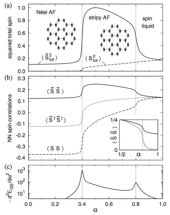
Figure 39: (a) Squared total spin of the 24-site cluster, normalized to its value in the fully polarized FM state, as a function of $0\leq\alpha\leq 1$ for $C>0$. The solid (dot-dashed) line corresponds to the rotated (original) spin basis. (b) The NN spin correlations: The solid (dot-dashed) line corresponds to a scalar product of the rotated (original) spins. The component of the correlation function matching the bond direction is indicated by a dotted line. This quantity is the same in both bases. The inset compares NN spin correlations (solid line) above $\alpha=0.5$ with longer range spin correlations up to third-nearest neighbors (dotted lines). (c) Negatively taken second derivative of the ground state energy with respect to $\alpha$. Its maxima indicate the phase transitions at $\alpha\approx 0.4$ and 0.8. Chaloupka et al. (2010).

It is further noteworthy that an applied uniform field in the spatially dependent rotated basis discussed above leads to a near saturation of the rotated ${\bf{\tilde{{\tau}}}}$ moments within the stripy antiferromagnetic phase Chaloupka et al. (2010). The phase diagram of this system has been recently explored in the presence of an external magnetic field Jiang et al. (2011) and at finite temperatures Reuther et al. (2011). We next survey the results found in those cases.

External Magnetic Field As was surveyed earlier, in Kitaev’s honeycomb model, the application of a magnetic field ${\bf{h}}$ along the $\langle 111\rangle$ direction leads to the appearance of a non-Abelian topological phase Kitaev (2006). Inspired by this, the authors of Jiang et al. (2011) investigated the phase diagram of the amended Hamiltonian

$$H_{HK+h}=H_{HK}-{\bf{h}}\cdot\sum_{i}{\bf{\tau}}_{i}$$ (200)

Physically such an effective magnetic field coupling to the pseudo-spins as in Eq. (106), can be brought about by, e.g., a magnetic field that couples to the original spin degrees of freedom. The found phase diagram is depicted in Fig. 40. As seen in Fig. 40, the transitions between the three zero-field phases present when $C>0$ and $0\leq\alpha\leq 1$ (Neel, stripy ferromagnet, and ferromagnetic spin liquid) persist yet with additional rich features. We comment on these below.

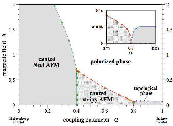
Figure 40: Ground-state phase diagram of the Heisenberg-Kitaev model with $C=1$ in Eq. (113). 1) in a magnetic field of strength $h$ along the direction $[111]$. Interpolating from the Heisenberg ($\alpha=0$) to Kitaev ($\alpha=1$) limit for small field strength, a sequence of three ordered phases is observed: a canted Neèl state for $\alpha<0.4$, a canted stripy Neèl state for $0.4<\alpha<0.8$, and a topologically ordered state for nonvanishing field around the Kitaev limit. All ordered phases are destroyed for sufficiently large magnetic field giving way to a polarized state. Jiang et al. (2011).

(1)  The canted and polarized phases At sufficiently large $h=|{\bf{h}}|$, the pseudo-spins become polarized along the applied field $\langle 111\rangle$ direction. For $h>0$, the Neel and stripy ferromagnetic states both become canted along this direction as well. As symmetry considerations indicate, and is numerically seen, the six-fold degeneracy of both the canted Neel state and the canted stripy antiferromagnet persist as $h$ is varied.

The transition between the canted Neel and polarized state as well as the transition between the canted stripy antiferromagnet and the polarized state are both continuous. By contrast, the transition between the canted Neel state and the canted stripy ferromagnet is a first order transition. Thus, the point of merger of the two critical lines separating the canted phases from the polarized states and the first order line separating the two canted phases from one another constitutes a viable tricritical point.

(2)  The topological spin liquid phase The Iridates offer the exciting prospect of potentially realizing a non-Abelian topological phase. As discussed earlier, in Eqs. (246, 247, 260) in his seminal work Kitaev (2006), Kitaev argued, via perturbative considerations, that the application of a magnetic field may lead to a gapfull phase with non-Abelian statistics.

Specifically, as reviewed in Section X.4, a field in the $[111]$ direction, leads to a third order perturbative term of the form of Eq.(247) Kitaev (2006). This additional three spin term in turn translates, in the bond algebraic technique which we will review in subsection X.3, to the Hamiltonian of Eq.(260) with additional terms that link next nearest neighbor Majorana fermions ($A_{ij}$ is non-zero for sites $i$ and $j$ that are next nearest neighbors). The model of Eq. (260) was quadratic and solvable. The additional bilinear resulting from the field led to the appearance of a mass and non-Abelian statistics.

To test this perturbative argument and to better understand the character of the non-Abelian phase and its potential realization in the Iridates, the authors of Jiang et al. (2011) numerically probed an even more general Hamiltonian that than of Eq.(200) that is given by

$$H_{HK+h+\kappa}=(H_{HK+h}-\kappa\sum_{ijk}\tau^{x}_{i}\tau^{y}_{j}\tau^{z}_{k}).$$ (201)

The $\kappa$ term in Eq.(201) extends over spin triads as soon in Fig. 41.

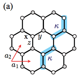
Figure 41: The honeycomb lattice spanned by unit vectors ${\bm{a}}_{1}=(1,0)$ and ${\bm{a}}_{2}=(1/2,\sqrt{3}/2)$ Jiang et al. (2011).

It was numerically established Jiang et al. (2011) (see Fig. 42)) that the non-Abelian phase obtained by setting $h=0$ (and $\alpha=1$) in the Kitaev model for $\kappa>0$ is adiabatically connected to the physical system of the Iridates in a magnetic field given by the Hamiltonian of $H_{HK+h}$ with $\kappa=0$. The critical field required to go to the polarized phase is seen to be monotonic and saturate when $\kappa$ is large. This is in accord with theoretical expectations as the Majorana fermion gap in the non-Abelian phase is monotonic in $\kappa$ and asymptotically tends to a constant for large $\kappa$ Jiang et al. (2011).

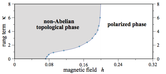
Figure 42: The constant $C=1$ in Eq. (113). Ground-state phase diagram of the Kitaev model ($\alpha$= 1) in the $h-\kappa$ plane, where $h$ is the strength of a magnetic field pointing in the 111 direction and $\kappa$ is the strength of a time-reversal symmetry breaking three-site term Jiang et al. (2011).

The transition between the non-Abelian phase and the polarized phase in the system of $H_{HK+h}$ appears to be continuous. Moreover, for any finite field $h\neq 0$ there is no direct transition between the canted stripy antiferromagnetic phase and the non-Abelian phase. It seems that within the $h\to 0$ limit, the two critical lines marking the (i) boundary between the stripy antiferromagnet and the polarized phase and (ii) the boundary between the topological spin liquid and the polarized phase may merge at a single multi-critical point near $\alpha\simeq 0.8$ (in agreement with the value found by Chaloupka et al. (2010)).

Finite temperature transitions Reuther et al. (2011) employed the pseudo-fermion renormalization group (PF-FRG) approach Reuther & Wolfle (2010); Reuther & Thomale (2011) to assess viable ordering at finite temperatures. The pseudo-spins are expressed as (pseudo-) fermi bi-linears and the resulting system is investigated perturbatively. The phase diagram resulting from their analysis is presented in Fig. 43. As we will discuss below, the critical cutoff scale $\Lambda_{c}$ was argued to emulate the ordering temperature.

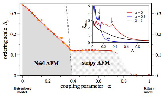
Figure 43: Ordering scale $\Lambda_{c}$ obtained from the FRG calculations for various coupling parameters. The constant $C$ in Eq. (113) was set here to unity. The dashed line indicates the crossover from dominant AFM to dominant s-AFM fluctuations as well as an extrapolation below the ordering transition down to $T=0$. A regime of enhanced numerical uncertainties is encountered near $\alpha\approx 0.8$. The inset shows the RG flow of the magnetic susceptibility versus frequency cutoff $\Lambda$. The arrows indicate the estimated ordering temperatures $\Lambda_{c}$ where the RG flow breaks down Reuther et al. (2011).

More generally, following Honerkamp & Salmhofer (2001), who noted that both the frequency cutoff $\Lambda$ and the temperature $T$ play the rule of infra-red cutoffs the key notion was to identify various frequency cutoff $\Lambda$ scales in the PF-FRG approach to correspond to physical temperature scales. This qualitative identification was motivated by direct finite $T$ calculations: this general correspondence was validated in the analysis of the high temperature susceptibility.

Curie-Weiss temperature In what follows $C=1$ in Eq. (113). It was found Reuther et al. (2011) that, at high temperatures, the ferromagnetic susceptibility adhered to the Curie-Weiss law

$$\chi\sim 1/(\Lambda-\Lambda_{CW}).$$ (202)

The thus extracted Curie-Weiss scale $\Lambda_{CW}>0$ for $\alpha\gtrsim 0.68$ (indicating an overall effective ferromagnetic coupling (as consistent with the ferromagnetic couplings in the Kitaev ($\alpha=1$ and $C>0$) limit)). Similarly, the observation of $\Lambda_{CW}<0$ for $\alpha\lesssim 0.68$ is consistent with the Heisenberg ($\alpha=0$) limit of Eq.(113). Such a change in the sign of the dominant exchange, as adduced from the dependence of the susceptibility $\chi$ on the cutoff $\Lambda$, is consistent with semi-classical analysis for which the Curie-Weiss temperature is given by Reuther et al. (2011)

$$\Theta_{CW}=-\frac{3}{4}+\frac{5}{4}\alpha.$$ (203)

In Eq. (203), a crossover from an overall ferromagnetic to antiferromagnetic behavior occurs at $\alpha=0.6$ (proximate to the value of $\alpha\simeq 0.68$ suggested by the dependence of $\chi$ on the cutoff). The variation of the effective Curie-Weiss cutoff scale $\Lambda_{CW}$ over the entire range of $\alpha$ values is provided in Fig. 44. Qualitatively, the dependence of $\Lambda_{CW}$ on $\alpha$ is similar to that of the semi-classical approximation of Eq. (203).

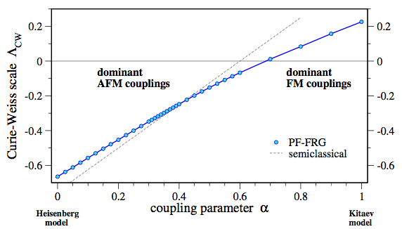
Figure 44: The constant $C=1$ in Eq. (113). The Curie-Weiss scale $\Lambda_{CW}$ obtained from fitting the inverse susceptibilities to a Curie-Weiss law for varying coupling parameter $\alpha$. Around $\alpha\approx 0.68$ the Curie-Weiss scale switches sign indicating a transition of the dominant exchange from antiferromagnetic ($\Lambda_{CW}<0$) to ferromagnetic ($\Lambda_{CW}>0$). Reuther et al. (2011).

Ordering temperatures The scale of the ordering temperatures $T_{o}$ was identified with the critical cutoff $\Lambda_{c}$ beyond which the Renormalization Group flow breaks down in the PF-FRG method Reuther et al. (2011), see Fig. 43 Reuther et al. (2011).

It is seen that within the Neel phase $(\alpha\simeq 0.4$) both the inferred (i) ordering temperature $T_{o}$ and (ii) the Curie-Weiss temperature $\Theta_{CW}$ scales are nearly linear in $\alpha$. By contrast, within the stripy ferromagnetic phase apart from the region near the transition into the spin liquid phase, the relevant ordering temperature $T_{o}$ (as suggested by the value of the critical cutoff scale $\Lambda_{c}$) is nearly $\alpha$ independent Reuther et al. (2011). Unlike the ordering temperature itself, $\Theta_{CW}(\alpha)$ varied approximately linearly in this range of $\alpha$ values of the stripy antiferromagnet phase. In the spin-liquid phase ($\alpha\gtrsim 0.8$), the ordering temperature $T_{o}=0$.

Assuming that both the Curie Weiss and ordering temperatures ($\Theta_{CW}$ and $T_{o}$) are related by an identical multiplicative scale factor to the cutoff scales $\Lambda_{CW}$ and $\Lambda_{c}$, the ratio $(|\Lambda_{CW}|/\Lambda_{c})$ is equal to the experimentally measured “frustration parameter” Ramirez (1994) ratio of $f=(|\Theta_{CW}|/T_{o}$) Reuther et al. (2011). This ratio is nearly constant ($f\approx 2$) in the Neel phase and monotonically diminishes in size as $\alpha$ is increased beyond the transition point ($\alpha\approx 0.4)$ into and throughout most of the stripy antiferromagnetic regime. Within the spin-liquid phase, $f$ diverges. In comparison to experiments Reuther et al. (2011), the measured frustration parameter for the iridate Na₂IrO₃ Singh & Gegenwart (2010) ($f\approx 8$) is far larger than the values adduced for the Heisenberg-Kitaev model in these phases. Earlier work has not examined finite temperature behavior the zig-zag or other phases which lie outside the $C>0$ and $0\leq\alpha\leq 1$ parameter regime. By invoking the self-duality transformation of Eq. (196) to the results of Reuther et al. (2011) and its adduced phase diagram above, one may ascertain the extended finite temperature phase diagram including the zig-zag phase (this is so as zig-zag phase is dual to the stripe antiferromagnet). Thus as the transition temperature $T_{o}$ in the stripy antiferromagnetic phase, as determined by thermodynamic measurements, is nearly constant as a function of the parameter $\alpha$ of Eq.(113), invoking the self-duality relations of Eqs. (196), one finds that the ordering temperature of the zig-zag phase is also nearly constant.

IX.12.6 Heisenberg-Ising Hamiltonians

Bhattacharjee & Kim (2011) noted that trigonal distortions around the Ir⁴⁺ ions can lead to significant crystal field effects. These crystal fields may splinter the three $t_{2g}$ orbital states into a degenerate doublet ($e_{1g}^{\prime}$ and $e_{2g}^{\prime}$) and a non-degenerate $a_{1g}$ state. Spin-orbit coupling may lead to a locking of the spin and orbital degrees of freedom and thus to the appearance of only two pertinent states, e.g., $|e_{1g}^{\prime}\downarrow\rangle$ and $|e_{2g}^{\prime}\uparrow\rangle$ where $\downarrow$ and $\uparrow$ denote the two possible values of the electronic spin along the axis of trigonal distortion; these replace the two states of Eq. (106). As before, these two states can be regarded as eigenstates of a pseudo-spin 1/2 operator.

Bhattacharjee & Kim, 2011 report that a uniform trigonal distortion is most consistent with the experimental results. With the aid of the pseudo-spin 1/2 operator discussed above, an effective model with Heisenberg (${\bf\tau}_{i}\cdot{\bf\tau}_{j}$) and Ising ($\tau^{z}_{i}\tau^{z}_{j}$) type interactions each of which of which contains nearest, next nearest, and next-next nearest couplings is constructed (i.e., a $\tilde{J}_{2}-\tilde{J}_{3}$ Heisenberg-Ising model). Resultant ground states, on the mean field level, include the zig-zag state.

Note that the models of Bhattacharjee & Kim (2011) and Kimchi & You (2011) which report to fit the experimental data (as well as, of course, the bare Heisenberg-Kitaev model that was reviewed earlier) can all be written in terms of a generalized $\tilde{J}_{2}-\tilde{J}_{3}-J_{2}^{I}-J_{3}^{I}$ type Heisenberg-Ising-Kitaev model which takes the form

$$H_{HIK}=H_{HK}-\tilde{J}_{2}\sum_{\langle\langle ik\rangle\rangle}{\bf\tau}_{i}\cdot{\bf\tau}_{k}-J_{3}\sum_{\langle\langle\langle il\rangle\rangle\rangle}{\bf\tau}_{i}\cdot{\bf\tau}_{l}$$

$$-J_{2}^{I}\sum_{\langle\langle ik\rangle\rangle}\tau_{i}^{z}\tau_{k}^{z}-J_{3}^{I}\sum_{\langle\langle\langle il\rangle\rangle\rangle}\tau_{i}^{z}\tau_{l}^{z}.$$ (204)

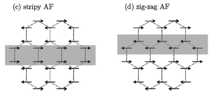
Figure 45: Crystal structure and possible antiferromagnetic-ordering patterns of the Ir sublattice. (c), and (d): three possible magnetic structures. In each case, the magnetic unit cell is the same as the structural unit cell. The shaded boxes highlight the stripy and zig-zag chain elements. Liu et al. (2011).

IX.12.7 Heisenberg-Kitaev $\tilde{J}_{2}-\tilde{J}_{3}$ Model

In Kimchi & You (2011), an extension of the bare Heisenberg-Kitaev Hamiltonian $H_{HK}$ [Eq. (113)] was introduced wherein additional next nearest neighbor ($\langle ik\rangle$) and next-next nearest neighbor ($\langle\langle il\rangle\rangle$) Heisenberg terms appear,

$$H_{\tilde{J}2J\tilde{3}} = C\Big{[}-2\alpha\sum_{\langle ij\rangle_{\gamma}}\tau_{i}^{\gamma}\tau_{j}^{\gamma}+(1-\alpha)\sum_{\langle ij\rangle}{\bm{\tau}}_{i}\cdot{\bm{\tau}}_{j}\Big{]}$$ (205)

$$+ (1-\alpha)[\tilde{J}_{2}\sum_{\langle\langle ik\rangle\rangle}{\bf\tau}_{i}\cdot{\bf\tau}_{k}+\tilde{J}_{3}\sum_{\langle\langle il\rangle\rangle}{\bf\tau}_{i}\cdot{\bf\tau}_{l}].$$

As $\alpha$ is varied from zero to unity, this extended system interpolates between an SU(2) symmetric limit to Kitaev’s honeycomb model. Heisenberg exchange type terms between next nearest neighbor and further away sites may arise, in the standard way, from high order processes including hopping processes and orbital overlaps Kimchi & You (2011). Indeed, Bhattacharjee & Kim (2011) found $\tilde{J}_{2}$ to be comparable to the nearest neighbor exchange $C$ (which following Kimchi & You (2011) has been typically set to unity in Eq. (205)).

An analysis of Eq. (205) was performed for the classical ground states Kimchi & You (2011) along similar lines to that of Nussinov (2001) to find that for general minimizing wave-vectors of the interaction kernel $\hat{V}({\bf k})$ of Eqs. (56, 150), spirals constitute the sole ground states. For commensurate minimizing wave-vectors, additional Neel, zig-zag type, and stripy ground states were found. This append the earlier discussed ground states found for the Heisenberg-Kitaev system at the point $\tilde{J}_{2}=\tilde{J}_{3}=0$. Notably, the zig-zag type phase in this model was found already when $C>0$ and $0\leq\alpha\leq 1$.

Exact diagonalization of the Hamiltonian of Eq. (205) was further performed and by employing all of the found eigenstates, the extended phase diagram mapped at finite temperatures. The authors of Kimchi & You (2011) suggest that the current experimental data may for both Na₂IrO₃ and Li₂IrO₃ when $\tilde{J}_{2}$ and $\tilde{J}_{3}$ as well as the Kitaev term may be significant (see table I in Kimchi & You (2011)). A moderate trigonal coupling enhanced both Heisenberg and Kitaev type terms as well as lead to additional (small) Ising interaction terms (i.e., $\tau^{z}_{i}\tau^{z}_{j}$) and Ising-Kitaev terms ($\tau^{\gamma}_{i}\tau^{z}_{j}$ with $\gamma$ set by the direction $(ij)$) and were not suspected to radically change the obtained results Kimchi & You (2011).

IX.12.8 Spin density functional theory calculations

Thus far, we reviewed the results as they pertain to the Heisenberg-Kitaev model of Eq. (113). Also first principle type spin density functional theory computations have been carried out, sans the reduction to a Heisenberg-Kitaev model, to directly ascertain possible orders of Na₂IrO₃ Liu et al. (2011). These calculations further suggested the existence of non-colinear (“zig-zag”) states different from the stripy antiferromagnet and that are lower in energy. The zig-zag states are found as ground staters for $C<0$; these states are promoted by inter-orbital exchange (see Section V.1.8 and Eq. (111) in particular) which is a dominant contribution Chaloupka et al. (2013).

To clarify the structure of the zig-zag states and their difference as compared to the stripy antiferromagnetic state, a comparison of these states is provided in Fig. 45. Aside from their presence in the Heisenberg-Kitaev model for $C<0$ in Eq. (113), as briefly alluded to earlier, such zig-zag states were also found in the phase diagram of the Heisenberg-Kitaev $\tilde{J}_{2}-\tilde{J}_{3}$ Model Kimchi & You (2011) also for $C>0$ and $0\leq\alpha\leq 1$.

IX.12.9 Experimental Results

Although, as we will now review, some preliminary results are suggestive, determining whether exotic aspects of the physics of the Heisenberg-Kitaev model of Eq.(113) are indeed materialized in the iridates of the A₂IrO₃ type still requires more effort.

We have by now alluded several times to one of the currently most promising maxims in that regard. Experiments suggest the presence of the zig-zag phase in the iridates Liu et al. (2011); Choi et al. (2012). As we reviewed above, this phase may be expected to be the pertinent one in the iridates Chaloupka et al. (2013) given the typical parameters that characterize the effective Heisenberg-Kitaev model and the dominance of Eq. (111). Furthermore, the dispersion computed for spin waves within the zig-zag phase Chaloupka et al. (2013) and the magnetic susceptibility are consistent with neutron scattering Choi et al. (2012) and magnetic susceptibility data Singh & Gegenwart (2010); Singh et al. (2012). These calculations for predictions concerning the Heisenberg-Kitaev model in its zig-zag phase Chaloupka et al. (2013) are also consistent with magnetic susceptibility measurements of both Na₂IrO₃ and Li₂IrO₃ Singh et al. (2012). Fig. (46) from Chaloupka et al. (2013), shows a comparison between the experimentally measured susceptibility as a function of temperature and that fittedwith empirically suggested parameter values for Na₂IrO₃ (as well as parameters for Li₂IrO₃).

Figure 46: INSERT FIG. 4 FROM  Chaloupka et al. (2013). The parameters are for Na₂IrO₃ are given by $(J_{1},J_{2})=(-20.9,-4.01)$ in Eq. (113) [or, equivalently, $\alpha=0.723$, $C=-14.46meV$ (corresponding to an angular parameterization with $\varphi$ in the second quadrant with $\tan\varphi\simeq 2.61$)] . The parameters for Li₂IrO₃ are given by $(J_{1},J_{2})=(-15.7,-5.3)$, or equivalently, $C=-12.15meV$and $\alpha=0.564$ (corresponding to $\tan\varphi\simeq-1.48$ with $\varphi$ in the second quadrant).

As discussed above, one of the key results of the finite temperature analysis of Reuther et al. (2011) was that, within the stripy antiferromagnetic phase, the transition temperature $T_{o}$, as determined by thermodynamic measurements, is nearly constant as a function of the parameter $\alpha$ of Eq.(113) [see Fig. 43] while the Curie-Weiss temperature varied smoothly with $\alpha$ [Fig. 44]. As first remarked above, invoking the self-duality relations of Eqs. (196), one sees that the same follows for the ordering temperature of the zig-zag phase.

An interesting set of experiments Singh & Gegenwart (2010); Liu et al. (2011); Singh et al. (2012) on Na₂IrO₃ and Li₂IrO₃ offers a consistent realization of this trend. In particular, in Singh et al. (2012) it was found that both Na₂IrO₃ and Li₂IrO₃ exhibit the thermodynamic signatures of a transition at $T_{o}\simeq 15K$. (Scattering measurements indicate that long range magnetic ordering, in Na₂IrO₃ is, as to be expected, nearly coincident and appears for $T\lesssim 13.3K$. Liu et al. (2011); magnetic susceptibility measurements (which have been fitted in Fig. (46)) similarly show a precipitous drop at $T\simeq 15K$ Singh & Gegenwart (2010).) [see Fig. 47 from Singh et al. (2012)].

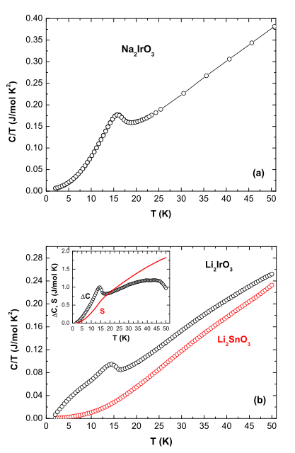
Figure 47: (a) The heat capacity divided by temperature $(C/T)$ versus the temperature $T$ data between $T$ = 1.8 K and 40 K for single crystals of Na₂IrO₃ and the heat capacity of Na₂SnO₃ as the lattice contribution $C_{lattice}/T$ versus $T$. The inset shows the $C/T$ versus $T$ data in $H=0$ and 7T applied magnetic field. (b) The difference heat capacity $\Delta C$ and difference entropy $\Delta S$ versus $T$ data between $T$ = 1.8 K and 40 K  Singh et al. (2012).

However, while Na₂IrO₃ has a Curie-Weiss temperature $\Theta_{CW}\simeq-125K$, its cousin Li₂IrO₃, with the lighter Li ion replacing Na, exhibited a far reduced Curie Weiss temperature of $\Theta_{CW}\simeq-33K$ [see Fig. 48 from Singh et al. (2012)].

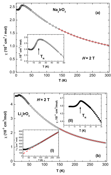
Figure 48: (a) Magnetic susceptibility $\chi$ versus temperature $T$ for Na₂IrO₃. The fit by the Curie-Weiss (CW) expression $\chi=chi_{0}+C/(T-\theta)$ is shown as the curve through the data. The inset shows the anomaly at the antiferromagnetic ordering. (b) $\chi$ versus $T$ for Li₂IrO₃. The solid curve through the data is a fit by the CW expression. The inset (I) shows the $1/\chi(T)$ data for Li₂IrO₃. The solid curve through the data is a fit by the CW expression and the dashed curve is an extrapolation of the fit to lower $T$ . The inset (II) shows the anomaly at the onset temperature of antiferromagnetic ordering Singh et al. (2012).

An initial possible interpretation of these results was that both Na₂IrO₃ and Li₂IrO₃ correspond (possibly with some additional terms) to a realization of Eq. (113) within the stripy antiferromagnet phase yet with two different values $\alpha$. This is further bolstered by the observation that the magnetic susceptibility $\chi(T)$ saturates at low temperatures Singh & Gegenwart (2010) to a large finite value: such a saturation is consistent with stripe type ordering. Resonant X-ray scattering measurements Liu et al. (2011) further indicate Bragg peaks that are inconsistent with a Neel state. These peaks may, however, be accounted for by structures similar to the stripy antiferromagnet or the somewhat similar zig-zag states. As noted earlier, from spin density functional calculations Liu et al. (2011) the zig-zag states were suggested to be lower in energy than the stripy antiferromagnetic states. Interestingly, as we reviewed in some detail above, the zig-zag states are ground states of the Heisenberg-Kitaev model within an extensive parameter regime. Notably, the inter-orbital $t_{2g}$-$e_{g}$ exchange processes [leading to Eq. (111)] may promote precisely the zig-zag phase of very likely experimental pertinence in the iridates Chaloupka et al. (2013).

The experimental results are thus consistent with some of the predictions of the Heisenberg-Kitaev model but, currently, more work (both theoretical and experimental) may be required to attain a more comprehensive picture. Accounts including (i) effective $C-J_{2}-J_{3}$ Heisenberg-Ising type models with interactions that may result from large diagonal couplings Bhattacharjee & Kim (2011) as well as (ii) $\tilde{J}_{2}-\tilde{J}_{3}$ Heisenberg-Kitaev models Kimchi & You (2011) may well better explain key features of the data.

In closing, we should note more rudimentary aspects that have been established in these materials. From the Curie-Weiss tails, it was determined that both Na₂IrO₃ and Li₂IrO₃ have an effective spin of $S_{eff}=1/2$ Singh & Gegenwart (2010); Singh et al. (2012). Both of these Iridates are Mott insulators. In Singh & Gegenwart (2010), it was found that, for $100K<T<300K$, the electrical resistivity data for Na₂IrO₃ is of the variable range hopping type as expected for localization by disorder; there is no sign of activated Arrhenius behavior. It was further seen that aside from a pronounced drop of the susceptibility at $T\simeq 15K$, there is a broad global maximum of the susceptibility at $T\simeq 23K$. This broad maximum in the susceptibility, the high temperature tail of the specific heat change (after lattice subtraction), and the entropy adduced with this specific heat data all suggest that short order persists beyond $T_{o}\simeq 15K$ up to higher temperatures. Some early, non thermodynamic, measurements of Li₂IrO₃ Felner & Bradaric (2002); Kobayashi et al. (2003). suggested the non-existence of magnetic order (for measured temperatures of $T>5K$) Felner & Bradaric (2002) and glassy behavior Kobayashi et al. (2003).

IX.13 Compass Heisenberg Models

The Heisenberg-Kitaev models studied in subsection IX.12 constitute a very special case of the more general Compass-Heisenberg models of Eq. (38). Non Heisenberg-Kitaev realizations of the Compass-Heisenberg models have not been less explored. Some key features of the 90^∘ compass Heisenberg model have been reported in Trousselet et al. (2010, 2012). As reviewed in section V.2, this model and its descendants may describe a placement of rectangular superlattice of vacancy centers on a diamond grid. The prominent effect of adding Heisenberg interactions was highlighted in Trousselet et al., 2012. Introducing arbitrarily weak Heisenberg interactions lifts the exponential degeneracy of the compass system and favor a particular ordering between the compass model rows (or columns). In the presence of Heisenberg interactions, only a two-fold degeneracy remains. The anisotropic compass interactions lead to a gap to spin wave excitations. In small clusters, the lowest energy excitations are those in which entire individual rows (or columns) are flipped. These excitations and related issues have been extensively investigated Trousselet et al. (2012).

X Kitaev Models & Quantum Computing

Recently, there has been much activity in the study of compass-related models as candidates for topological quantum memories Kitaev (2003, 2006). In such a topological memory, quantum states can in principle be encoded fault tolerantly – i.e., be protected against decoherence Shor (1996); Kitaev (2003, 2006); Dennis et al. (2002). This aspect of fault tolerance motivates this activity. Assuming that errors are of a local nature, topological quantum memories are intrinsically stable because of physical fault-tolerance to weak, quasi-local, perturbations.

In this section, we review two of the prototypical models which were invented to describe the basic principles of topological quantum computing Kitaev (2003, 2006). As we will see, one of these models, Kitaev’s toric code model, is essentially a pure Ising gauge theory. Its excitations are anyons that obey Abelian statistics. It appears as a limiting form of the Kitaev honeycomb model which is far richer and enables non-Abelian quantum computing. Kitaev’s honeycomb model is exactly the compass model on a hexagonal lattice, introduced in Sec. II in Eq. (13), where the non-Abelian excitations arise in presence of an additional magnetic field.

The key feature of these models is that possess these very interesting physical properties while still being exactly solvable, as will be explained in Sec. X.2 for the bare Kitaev model [and in Section X.4 for an extended variant in the presence of a magnetic field (or, more precisely, additional term involving the products of three neighboring pseudo-spins that supplant the two-spin interactions in Eq. (13)]. This sets these Kitaev models apart from the generic compass-type model. To introduce the general notions and to put the exciting features of the Kitaev models in perspective, we first briefly review anyonic statistics, braiding and fusion rules while keeping the focus on compass-Kitaev models. For an in-depth review of topological quantum computing we refer to Preskill (2004); Nayak et al. (2008).

X.1 Basic Notions of Statistics

A potent prediction of quantum mechanics is that identical particles must generally be fermions or bosons. In its simplest form one can consider a many body wavefunction $\psi(r_{1},...,r_{N})$ and the effect of permutations on it. If a permutation operator $P_{12}$ that permutes two particles (particles number 1 and 2) commutes with the Hamiltonian ($[H,P_{12}]=0$) then we can simultaneously diagonalize both the Hamiltonian and $P_{12}$. Such a relation is guaranteed when particles 1 and 2 are identical to one another and thus appear symmetrically in the Hamiltonian. Formally, one may view the operation of $P_{12}$ (and its square) as the spatial rotation of one particle around the other or the as the braiding of the world line of one particle around another, see Fig 49.

Conceptually, $P_{12}^{2}$ can be emulated by the rotation of one particle (say particle 1) about the other (particle 2) by 360^o. In three and higher spatial dimensions, the permutation operator is its own inverse ($P_{12}^{2}=1$) and consequently these are the only two generic possibilities of bosonic ($P_{12}|\psi\rangle=|\psi\rangle$) or fermionic statistics ($P_{12}|\psi\rangle=-|\psi\rangle$. Similarly, for general pairwise permutations $P$, one has that $P^{2}\psi(r_{1},r_{2},...,r_{N})=\psi(r_{1},r_{2},...,r_{N})$ and consequently $P=\pm 1$.

X.1.1 Anyons and Braiding

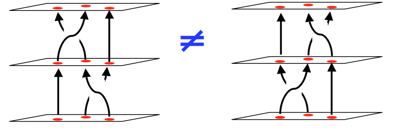
Figure 49: Braiding in two-spatial dimensions. If a braid group is non-Abelian (non-commutative) then the order of the braiding operations is important. The statistics in such cases are encoded in matrix representations of braid group. (Schematic courtesy of S. Simon.)

As first realized by Leinass and Myrheim, Leinaas & Myrheim (1977) in two spatial dimensions (or 2+1 space-time dimensions), however, the situation is considerably richer. In two spatial dimensions, the rotation of one particle around the other (emulating the permutation) need not be the same for clock-wise and counter-clockwise directions. Unlike the case in three spatial dimensions when a clockwise rotation can be converted into a counter-clockwise rotation depending on whether we are looking at the rotation from above or below the plane where the rotation takes place, in two spatial dimensions, a directionality can be associated with such a braiding operation, see Fig 49. In higher dimensions (e.g., three spatial or 3+1 space-time dimensions), a double exchange of two particles along a path is topologically equivalent to an exchange along a topologically equivalent path which is shrunk to the origin and thus the wavefunction must be unaltered.

Thought about equivalently, in 2+1 space-time dimensions braiding operations can have non-trivial topologies just as shoe string can be tied in three dimensions (and only in three dimensions). In higher space-time dimensions, just as shoe laces can always untied, particle world lines cannot lead to non-trivial topologies and the only possibilities are (especially so for gapped systems) those of fermionic and bosonic statistics.

Anyons are particles or excitations that are neither bosons nor fermions – hence the name any-ons Leinaas & Myrheim (1977); Wilczek (1982a, b). It is useful to define them formally by considering the configuration space ${\cal{C}}_{N}$ associated with $N$ identical particles that reside on the spatial manifold ${\cal{M}}_{N}$ Leinaas & Myrheim (1977). This space is given by

$${\cal{C}}_{N}=\frac{{\cal{M}}_{N}/{\cal{D}}}{S_{N}},$$ (206)

where ${\cal{M}}_{N}/{\cal{D}}$ refers to the removal of the space of singular configurations ${\cal{D}}$ (where two or more particles coincide) from the space ${\cal{C}}_{N}$. The division of the quotient group by the permutation $S_{N}$ group of $N$ particles is carried out in order to reflect the indistinguishability of the identical particles. Within the path integral formulation, a correspondence exists between the possible unitary irreducible representations of the first homotopy groups $\pi_{1}({\cal{C}}_{N})$ of the configuration space ${\cal{C}}_{N}$ and the viable statistics is seen. Specifically in two spatial dimensions, the first homotopy is given by the braid group $\pi_{1}({\cal{C}}_{N})=B_{N}$ of $N$ particles whereas in higher dimensions it is equal to the permutation group, $\pi_{1}({\cal{C}}_{N})=S_{N}$. Wu (1984)

The generators ${\cal{T}}_{i}$ of all of these homotopy groups (both braiding and permutations) that interchange particles at sites $i$ and $(i+1)$ satisfy the relations

$${\cal{T}}_{i}{\cal{T}}_{j}={\cal{T}}_{j}{\cal{T}}_{i},~{}~{}~{}~{}|i-j|\geq 2,$$

$${\cal{T}}_{i}{\cal{T}}_{i+1}{\cal{T}}_{i}={\cal{T}}_{i+1}{\cal{T}}_{i}{\cal{T}}_{i+1}.$$ (207)

For the permutation group, a double interchange corresponds to the identity ${\cal{T}}_{i}^{2}=1$; this additional constraint leads to a subgroup of the braiding group. Specifically, this constraint enables the permutation group to only have the well known $N!$ elements. By contrast, the braiding group is continuous.

It is instructive to consider one-dimensional irreducible (or scalar) representations of these groups. Whereas there are only two possible irreducible scalar representations of the permutation group $S_{N}$ (namely the trivial bosonic representation (where it is everywhere the identity 1) and the fermionic representation where it is given by $(-1)^{P}=\pm 1$ for even/odd permutations $P$), there is a continuous set of possible representations for the braid group $B_{N}$ wherein ${\cal{T}}_{j}=e^{i\theta}$. As it must, the braiding group representation $B_{N}$ includes ($\theta=0,\pi)$ the fermionic and bosonic statistics of the permutation $P_{N}$ representation as a subgroup. For such scalar representations, the ordering of the braiding operations is clearly unimportant. These braiding representations thus correspond to Abelian anyons.

One of the simplest realizations of such anyonic statistics is for (Abelian) Fractional Quantum Hall systems. In, e.g., the $\nu=1/3$ state, under the exchange of two excitations the wavefunction can acquire a phase of $\theta=\pm 2\pi/3$. That is, revolving one quasi-particle around another leads to the change of phase $|\psi\rangle\to e^{\pm 2\pi i/3}|\psi\rangle$. The fractional phase here of $2\pi/3$ may be seen to reflect a statistical Aharonov-Bohm effect Aharonov & Bohm (1959); Kivelson & Rocek (1985) associated with the fractional quasi-particle charge $q=\pm e/3$ with $e$ the electron charge Laughlin (1983); Goldman & Su (1995).

X.1.2 Non-Abelian Anyons

Non-Abelian topological excitations display non-trivial anyonic statistics Moore & Read (1991); Nayak et al. (2008); Stern (2010); Ahlbrecht et al. (2009). The end result following a rotation of one anyon around another generally depends on the order in which the rotations have been done, see, e.g., Fig 49. In such a case, the braid group is non-commutative. Such anyons lie at the heart of quantum topological computing schemes: in a remarkable work Freedman et al. (2002), it was illustrated that particular sorts of non-Abelian anyons allow universal quantum computation.

For non-Abelian anyons, a rotation of one particle around another (or braiding of their world lines) does not merely lead a change of the wavefunction by a phase. Rather, more generally, when non-Abelian anyons are wound around one another there is a unitary operator $U$ that leaves the system with the same energy as it must for identical particles but, however, leads to another physical state, $|\psi\rangle\to U|\psi\rangle$. If the unitary operators $U_{ab}$ corresponding to different exchanges of particle $a$ about particle $b$ do not commute (i.e., $[U_{ab},U_{cd}]\neq 0$ or $[U_{ab},U_{ac}]\neq 0$) then the system exhibits non-Abelian statistics. Formally, in Eq. (207), in such cases, the elements ${\cal{T}}_{i}$ are non-commuting unitary matrices that act on a degenerate space of states. Non-local operators are associated with the braiding of such anyons. As we will briefly elaborate on later, the corresponding braiding rules describe the different ways in which anyons can behave collectively, that are yet locally indistinguishable. For the anyonic character of these topological excitations (or defects) to be unambiguous, it is important that they can be localized so that braiding operations (and thus statistics) are well defined. Such a localization of anyonic excitations generally appears in gapped systems. Thus, the typical size of the anyons ($l_{anyon}$), set by the inverse of the requisite energy gap for their creation, must be far smaller than the scale of the their separation ($R$) during braiding operations, $l_{anyon}\ll R$.

To briefly make a connection with our discussions thus far in earlier sections, we remark that defects associated with the restoration of intermediate (or $d-$ dimensional) symmetries similar to those discussed in Section VI can exhibit anyonic statistics and non-trivial topological conservation laws. As elaborated elsewhere Nussinov & Ortiz (2009c), in systems including many compass models (including Kitaev’s), $d=1$ symmetry operations which link different ground states to another can be viewed as a process involving the creation and transport of virtual anyons (more precisely, members of pair formed by an anyon and an antianyon) around $d=1$ dimensional loops followed by an annihilation. On a finite size system, these degeneracy between states related to one another by operations involving such a transport of anyons can be lifted by corrections that are exponentially small in the system size (i.e., scale as $O(e^{-cL})$ with the constant $c>0$ and $L$ the linear system size along which the anyon and anti-anyon tunnel and recombine).

X.1.3 Fusion of Anyons

Besides braiding, fusion is the other key process for anyons. A well-known example of fusion is that bringing together two fermions gives a boson. The generalization of this notion to anyons leads to “fusion rules” that are of the form

$$a\times b=\sum_{c}N_{ab}^{c}c,$$ (208)

where the non-negative integer $N_{ab}^{c}$ denotes the number of distinct ways in which the anyons $a$ and $b$ may be fused together to form the anyon $c$. A notable property of fusion is its associativity,

$$(a\times b)\times c=a\times(b\times c).$$ (209)

When these anyons are Abelian, the fusion outcome is unique. For non-Abelian anyons there are multiple fusion channels: if there exists a pair $(a,b)$ for which $\sum_{c}N_{ab}^{c}>1$ then the anyons $a$ and $b$ are non-Abelian. Therefore the fusion outcome of two non-Abelian anyons is non-unique.

Hilbert spaces can be encoded with anyons whose number increases with the Hilbert space dimension. The fusion rules and associated quantum dimensions $\{d_{q}\}$ of quasi-particles of type $q$, determine the total dimension of the Hilbert space that can be encoded with a given set of anyons. The ground state degeneracy for $n_{q}$ quasi-particles scales as $d_{q}^{n_{q}}$. This exponential degeneracy factor in non-Abelian systems (wherein $d_{q}>1$) leads to an additive contribution to the entropy that scales as $S_{anyon}=n_{q}k_{B}\ln d_{q},$ with $k_{B}$ the Boltzmann constant. This entropy carried by the individual quasi-particles may allow for anyonic adiabatic cooling – an effect predicted in Gervais & Yang (2010).

X.1.4 Majorana Fermions

Majorana fermions Majorana (1937) appear in many systems. Formally, similar to the real ($a$) and imaginary ($b$) parts of a complex number $(z=a_{1}+ia_{2})$ for which $a_{1}=(z+z^{*})/2$ and $a_{2}=i(z^{*}-z)/2$), the two operators $c_{1,2}$ being the ”real” and ”imaginary” parts of a fermionic operator (i.e., $c_{1}=(d+d^{\dagger})/2$ and $c_{2}=i(d^{\dagger}-d)/2$, with $d^{\dagger}$ and $d$ being Fermi creation and annihilation operators) satisfy the Majorana algebra. By that, we mean that the operators $\{c_{j}\}$ satisfy the following relations that actually define a Majorana-Fermi algebra:

$$\{c_{j},c_{p}\} = 0~{}\mbox{for}~{}j\neq p$$

$$c_{j}^{2} = \frac{1}{2},$$

$$c_{j}^{\dagger} = c_{j},$$ (210)

where $\{c_{j},c_{p}\}$ denotes the anticommutator of two Majoranas, labeled by $j$ and $p$. One of their key physically defining features is that (as $c_{j}^{2}$ is a constant) the parity of number of fermions is important yet not the actual number of particles itself. Similarly, the creation or annihilation of a Majorana fermion amount to the same operation ($c_{j}=c_{j}^{\dagger}$) – or stated more colloquially, a Majorana fermion is its own anti-particle.

From this it is seen that one may represent ($2n)$ Majorana fermions in terms of $n$ fermions or vice versa. Majorana fermions offer one of the simplest realizations of the particles that have non-Abelian statistics Nayak et al. (2008); Rowell et al. (2009), as will become explicit in Section X.4 where we review the non-Abelian phase of the Kitaev model.

Such statistics are thought to occur in the $\nu=5/2$ fractional Quantum Hall state, as first suggested by Moore and Read Moore & Read (1991) by investigating their conjectured $\nu=5/2$ wavefunction. Nayak and Wilczek later illustrated that each quasi-particle in this state carries a zero energy Majorana fermion Nayak & Wilczek (1996). Currently, it is still not experimentally known whether non-Abelian statistics indeed occurs in this state.

While, currently, it is not clear if Majorana fermions exist as fundamental particles –neutrinos might possibly offer such a realization– there is an increasing number of condensed matter systems in which Majorana fermions appear as excitations Wilczek (2009); Franz (2010); Ivanov (2001); Read & Green (2000); Lee et al. (2007); Schnyder et al. (2008); Alicea (2010).

Similar Majorana fermion quasi-particles were theoretically found in superconductors with a $p_{x}+ip_{y}$ gap function by Read and Green Read & Rezayi (1999). Ivanov Ivanov (2001) investigated the quasi-particle statistics by examining adiabatic change in these superconductors. This enabled an explicit matrix representation of braid group element. Kitaev illustrated that non-Abelian anyons with zero energy Majorana modes appear in the Kitaev honeycomb model when the Chern number is odd Kitaev (2006). All in all, an extraordinary amount of work was devoted to these viable fractional Quantum Hall and other states that may exhibit non-Abelian statistics Willet et al. (1987); Xia et al. (2004); Eisenstein et al. (2002); Moore & Read (1991); Read (2009); Nayak & Wilczek (1996); Ivanov (2001); Stern et al. (2004); Read & Green (2000); Read & Rezayi (1999); Levin & Wen (2005); Wen (1993); Greiter et al. (1991); Morf (1998); Storni et al. (2010); Toke et al. (2007); Rezayi & Haldane (2000); W js & Quinn (2006); Feiguin et al. (2008). As alluded to above, $p-wave$ superconductors Ivanov (2001); Nayak et al. (2008) may display non-Abelian statistics. Non-Abelian anyons might potentially occur also in cold-atom systems Cooper et al. (2001); Gurarie & Radzihovsky (2007), topological insulator or superconductor based systems Hasan & Kane (2010); Fu & Kane (2008, 2009); Nilsson et al. (2008); Beenakker (2011) and, notably, possibly also in semi-conductor wires Alicea (2010); Alicea et al. (2011) and semi-conductor/(s-wave) superconductor hybrids Sau et al. (2010).

X.1.5 Fused Magetic and Electric Charges – Dyons

Armed with two different types of particles, for instance a particle with electric charge $q$ and another particle with a magnetic flux $\phi$ and their relative statistics, see Fig. 50, one can discuss all possible composites of these basic electric and magnetic particles. In one of the simplest instances of an electromagnetic type theory (or $U(1)$ theory) with magnetic and electric charges, the Aharonov-Bohm phase associated with the rotation of a particle of charge $q$ about a particle carrying a flux $\phi$, wherein the system state $|\psi\rangle\to\exp[2\pi iq\phi]|\psi\rangle$, leads to a non-trivial statistics when $q\phi$ is not an integer.

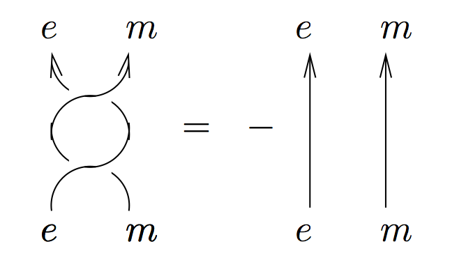
Figure 50: Relative statistics between electric and magnetic charges.

The most basic composite to consider in this context is a dyon – a ”molecule” composed of an electrical and a magnetic particle that have been brought together and fused. As the magnetic particles have trivial statistics amongst themselves – the Aharonov Bohm phase associated with transporting one magnetic particle around another is zero – and similarly all electrically charged particles have trivial mutual statistics, the only complication that can arise when consider the mutual statistics of two dyons is that arising from revolving the charge $q$ about the flux $\phi$. That leads to a uniform phase factor of $\exp[2\pi iq\phi]$. That is, the dyons can have a non-trivial fractional statistics among themselves.

Perhaps the simplest anyons are those that arise in an Ising (or $Z_{2}$) theory. Here, there are only two possible values for the electrical and magnetic charges. The electrical charge, which is henceforth denoted by $e$, can assume a value of $\pm 1$ and similarly the magnetic charge $m$ can assume be $\pm 1$. Revolving an electrical particle around a magnetic particle entails an Aharonov Bohm phase of $\exp[i\pi]=-1$, see Fig. 50.

In this case, there are only 4 possible basic particle type sectors, which sometimes are referred to as superselection sectors. These are given by (i) $e$ (the electric charge), (ii) $m$ (the magnetic charge), (iii) a dyon $\epsilon$ composed of a hybrid of an electric and a magnetic charge, and (iv) the vacuum (devoid of particles) which is denoted by $I$.

The magnetic particles are bosons relative to one another – there is no phase change in revolving a magnetic particle around another magnetic particle. Similarly, the electrical charges are bosons, the dyons are fermions. Formally one also associate vacuum ”particles” to $I$, in which case they are bosonic. The mutual statistics of these four particle types relative to one another is very simple. As stated earlier, revolving an electrical charge around a magnetic charge and also the converse (a magnetic charge around an electrical charge) entail a relative phase of $-1$. Similarly, revolving a magnetic particle around a dyon or an electrical charge around a dyon both involve a phase factor of $-1$.

One may similarly ask what occurs when we fuse two particles together – this is after all what the rather formal sounding name of ”fusion rules” aims to convey. One can consider for example how two electric charges behave when they are fused into a hybrid unit. In an Ising theory, two identical charges (no matter what charge it were $e=\pm 1$) would cancel each other and behave like no charge at all (the vacuum). This is formally encapsulated by the fusion rule

$$e\times e=I.$$ (211)

In a similar manner,

$$m\times m=I,$$

$$e\times m=\epsilon,$$

$$m\times e=\epsilon.$$ (212)

We note, for completeness, that the above fusion rules are augmented the universal trivial relations,

$$I\times I=I,~{}I\times e=e,~{}I\times m=m,~{}I\times\epsilon=\epsilon,$$ (213)

(and any other fusion with the identity matrix in other systems). We will not repeat again the trivial fusion rule with the identity in our future discussions; these are always to be understood.

As noted earlier, and is fleshed out in the particular example of the fusion rules above, for Abelian anyons, the product of the fusion of any pair of particles (on the lefthand side of Eqs. (211,212)) leads to a single unique particle (on the righthand side of these equations). In terms of Eq. (208), in Eq. (211,212) there always exists only a single channel for all possible ways of fusion.

As we will review in the upcoming sections, the fusion rules of Eqs. (211,212) precisely appear in the so-called Toric Code Model Kitaev (2003) and, by extension, in Kitaev’s honeycomb model in its Abelian phase Kitaev (2006). Such fusion rules- in particular those for richer non-Abelian counterparts (as in, e.g., the non-Abelian phase of Kitaev’s honeycomb model) that may lead to several possible fusion products and enable universal computation – form a cornerstone of various topological quantum computing schemes. The basic idea underlying topological quantum computing is that of preparing particular initial states with such particles (invoking, in effect, the fusion rules), performing calculations via unitary gates that employ braiding of these particles, and performing measurements by fusion Kitaev (2006). As alluded to above, such particles (both Abelian and non-Abelian) appear in Kitaev’s model which we now discuss.

X.2 Kitaev-Compass Model – Features

The 120^∘ compass model on the two-dimensional honeycomb lattice was introduced by Kitaev, 2006 and is often simply referred to as the Kitaev Honeycomb Model. Because of its central relevance to all that follows, we reiterate here that the Kitaev-compass Hamiltonian $H_{\varhexagon}^{K}$, as defined in Sec.II.1.2 and illustrated in Fig. 4 is given by Eq. (13) which we write anew,

$$H_{\varhexagon}^{K}= - J_{x}\sum_{\begin{smallmatrix}\bm{e}_{1}-&\\ {\sf bonds}&\end{smallmatrix}}\tau^{x}_{i}\tau^{x}_{j}-J_{y}\sum_{\begin{smallmatrix}\bm{e}_{2}-&\\ {\sf bonds}&\end{smallmatrix}}\tau^{y}_{i}\tau^{y}_{j}$$ (214)

$$- J_{z}\sum_{\begin{smallmatrix}\bm{e}_{3}-&\\ {\sf bonds}&\end{smallmatrix}}\tau^{z}_{i}\tau^{z}_{j},$$

where the operators ${\bm{\tau}}=(\tau^{x},\tau^{y},\tau^{z})$ represent (pseudo-) spin 1/2 degrees of freedom on neighboring vertices of a honeycomb lattice, labeled by $i$ and $j$. The lattice links may point along three different directions, labeled by $\bm{e}_{1}$, $\bm{e}_{2}$ and $\bm{e}_{3}$, where the angle between the three unit lattice vectors is $120^{\circ}$. Re-expressed in the explicit form of a compass model

$$H_{\varhexagon}^{K} = -\sum_{i,\gamma}J_{\gamma}\tau^{\gamma}_{i}\tau^{\gamma}_{i+\bm{e}_{\gamma}}$$ (219)

$$with\left\{\begin{array}[]{l}\{\tau^{\gamma}\}=\{\tau^{x},\tau^{y},\tau^{z}\}\\ \{J_{\gamma}\}=\{J_{x},J_{y},J_{z}\}\\ \bm{e}_{\gamma}=\bm{e}_{x}\cos{\theta_{\gamma}}+\bm{e}_{y}\sin{\theta_{\gamma}}\\ \{\theta_{\gamma}\}=\{0,2\pi/3,4\pi/3\}.\end{array}\right.$$

As we will review in Section X.6, in the limit of strong anisotropy, the Kitaev compass model on the honeycomb lattice (panel (A) of Fig. 51) reduces to another well known model in topological quantum computing- the “Toric Code” model (panel (B) of Fig. 51).

By its very nature, Kitaev’s honeycomb model is very similar to the $90^{\circ}$ compass models and other $120^{\circ}$ models. However, the Kitaev-compass system has a number of very remarkable properties. These can be assessed in a crisp manner because the model is exactly solvable: it can be mapped exactly onto a system of non-interacting Majorana (as well as Dirac) fermions, as will be detailed in Sec. X.3.2. This allows the derivation of all of the beautiful topological characteristics – its gapped bulk states, computable Chern numbers and Majorana excitations. Moreover, it will make evident that these Majorana excitations are coupled to a gauge field which embodies the topological charges, i.e., magnetic and electric like charges as introduced in Sec. X.1.

For future purposes it is useful to define an extension to this Hamiltonian $H_{\varhexagon}^{h}$, which actually becomes relevant if the model is studied in an external field $h$. This term involves three pseudo-spins on sites $i$, $j$ and $k$, and is the of form

$$H_{\varhexagon}^{h} = -\kappa\sum_{ijk}\tau^{x}_{i}\tau^{y}_{j}\tau^{z}_{k}$$ (220)

where the sum over $ijk$ is a sum over all sites connected by the two links $\langle ij\rangle$ and $\langle jk\rangle$. So here the link $\langle ij\rangle$ connects neighboring sites $i$ and $j$, similarly for $\langle jk\rangle$, but sites $i$ and $k$ are next nearest neighbors. This form of the Hamiltonian might seem rather particular at this point, but when adding it the model will stay exactly solvable. This term is essential to drive the Kitaev-compass Hamiltonian from a ground state with Abelian excitations to a state with non-Abelian ones, as will be discussed in Sec. X.4

The Kitaev-compass model reduces to the toric code model in the limit in which one coupling constant is far larger than all of the rest, e.g., $|J_{z}|\gg|J_{x,y}|$. The excitations in the toric code model, reviewed in Sec. X.6 precisely have magnetic and electric charges introduced in Sec. X.1.

As we reviewed earlier, compass systems such as Kitaev’s (and its extensions) may, e.g., be implemented by atoms in optical lattices Lewenstein et al. (2007); Duan et al. (2003) and cavity and ion trap systems Kay & Angelakis (2008); Trousselet et al. (2012); Schmied et al. (2011). By focusing on the low energy subspace (in a spirit somewhat similar to that of Section V.4) of magnetic clusters, Wang (2010) suggested that Kitaev’s model may be constructed via magnetic clusters on a honeycomb lattice. A proposal for experimentally constructing this system via superconducting quantum circuit elements was advanced in You et al. (2010). As we discussed in Section V.1.8, Kitaev-Heisenberg systems might describe the Iridates.

X.2.1 Relation to Topological Insulators

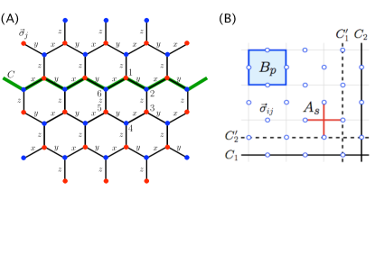
Figure 51: (A) Kitaev’s model on a honeycomb lattice and three types of bonds. On each vertex there is an $S=1/2$ degree of freedom indicated by a Pauli matrix $\vec{\sigma}_{j}$ (see text). (B) Elementary plaquette $B_{p}$ and star $A_{s}$ interaction terms in Kitaev’s Toric code model. Hollow circles in the bonds (links) represent an $S=1/2$ degree of freedom, while thick (dashed or solid) lines represent topological ($d=1$) symmetry operators (see text). Nussinov & Ortiz (2008a).

In many regards, Kitaev’s model furnishes an elegant and exactly solvable realization of a topological insulator Zhang (2008); Kane & Mele (2005b, a); Bernevig & Zhang (2006); Bernevig et al. (2006); Moore & Balents (2007); Roy (2009); Fu et al. (2007); Fu & Kane (2007). Topological insulators are systems that are gapped and insulating in the bulk yet due to topological characteristics harbor metallic, zero-energy, edge-states at the system’s boundaries. Due to topology, these edge-modes are robust and may retain their metallic character notwithstanding the introduction of disorder.

The class of topological insulators should include the integer quantum Hall states, which occur in 2D systems in which time-reversal symmetry is broken due to the presence of a magnetic field. Their quantum spin-Hall counterparts –the topological insulators mentioned above which can be realized in semiconductors with large spin-orbit coupling– time reversal symmetry remains unbroken Kane & Mele (2005b, a); Bernevig & Zhang (2006); Bernevig et al. (2006); Moore & Balents (2007); Roy (2009); Fu et al. (2007); Fu & Kane (2007). Similar to the integer quantum Hall systems the Kitaev-compass model exhibits sharp topological quantities such as the Chern number Avron et al. (2003); Chern (2010), which characterize two dimensional systems of free fermions with an energy gap. In integer quantum Hall systems, the Chern number is just the magnetic filling factor. Similar to other topological insulators, the Kitaev-compass model exhibits gapped phases in the bulk with concomitant gapless chiral modes: In the presence of a magnetic field, the Kitaev-compass model exhibits chiral edge-modes of a Majorana fermion character.

X.2.2 Majorana Excitations

The existence edge-states in the Kitaev model constitutes an analogue to quantum Hall systems and other topological insulators. However, in integer quantum Hall systems, the edge-modes are of bona fide fermions and not Majorana fermions. Its is the Majorana character of the excitations that in principle enables the aforementioned fault tolerance relative to all local fluctuations – ”errors” in the setting of quantum computing. The excitations of the Kitaev model flesh out the notions of anyonic statistics introduced in section X.1 and afford very crisp realizations of non-trivial topology. Kitaev’s model realizes fusion rules such as those of Eqs. (211,212).

The system also realizes one of the simplest examples of exotic ideas concerning fractionalization in strongly correlated electronic and spin systems. In its Abelian phase, the magnetic and electric excitations in the model may, respectively, be viewed Sachdev (2009) as counterparts of vison and spinon excitations in theories of doped quantum antiferromagnets Senthil & Fisher (2001) with relative ”semionic” statistics which requires that when an excitation of one type is moved around another it picks up a phase factor of $(-1)$.

It should be stressed that while the existence of excitations of Majorana-type is a special feature of the Kitaev-compass model, it is not necessarily an unique feature. In special situations three dimensional topological insulators may also exhibit Majorana fermion type of excitations, for instance ton their surface when placed at an interface with a superconductor Linder et al. (2010). Majorana fermions may also manifest in some of the systems that we earlier referred to in the context of non-trivial statistics: the fractional quantum Hall systems such that of the state of filling fraction $\nu=5/2$ Read & Green (2000), at cores of half-vortices in $p$-wave superconductors Ivanov (2001) and in semi-conductor Alicea (2010); Alicea et al. (2011) and semi-conductor/($s$-wave) superconductor systems Sau et al. (2010).

X.3 Kitaev-Compass Model – Abelian Phases

As was emphasized earlier, the Kitaev-compass model is exactly solvable in its ground state sector, for any set of coupling constants $J_{x}$, $J_{y}$ and $J_{z}$. The original solution in Kitaev, 2006 hinged on introducing several Majorana fermion degrees of freedom per site and making a projection on to a physical Hilbert space and symmetrization. Later approaches invoked a Jordan-Wigner (JW) transformation in two dimensions Chen et al. (2007); Chen & Nussinov (2008); Feng et al. (2007); Kells et al. (2009), perturbative methods, e.g., Vidal et al. (2008) and slave fermion methods Burnell & Nayak (2011); Schaffer et al. (2012). Another approach, which will be followed here, is based on the direct use of a bond algebra Nussinov & Ortiz (2009b). It is rather straight-forward and keeps directly track of the local symmetries that the Hamiltonian harbors, which are crucial to the solutions of $H_{\varhexagon}^{K}$ (and the same model augmented by $H_{\varhexagon}^{h}$). The explicit solution via the JW transformation Chen & Nussinov (2008) largely inspired the bond algebraic approach, but it is not as direct. The advantage of the bond algebraic method is that it enables the solution without enlarging the Hilbert space and making subsequent projections. Nor does it use at intermediate steps non-local string operators as in the Jordan-Wigner transformation.

X.3.1 Bond Algebra, Symmetries, and Anyonic Charge

In the Kitaev-compass Hamiltonian $H_{\varhexagon}^{K}$ three types of bonds $\{b_{jk}\}$ appear

$$\tau^{x}_{j}\tau^{x}_{j+\bm{e}_{1}},\ \tau^{y}_{j}\tau^{y}_{j+\bm{e}_{2}}\ \ and\ \ \tau^{z}_{j}\tau^{z}_{j+\bm{e}_{3}},$$ (221)

where $\{\bm{e}_{1},\bm{e}_{2},\bm{e}_{3}\}$ are unit vectors along the three directions of the hexagonal lattice. In terms of bond operators the Hamiltonian is

$$H_{\varhexagon}^{K}=\sum_{\langle jk\rangle}J_{jk}b_{jk},$$ (222)

with, as in Eq. (219), $J_{jk}=J_{x},J_{y}$ or $J_{z}$ depending on the orientation of bond $\langle jk\rangle$ along one of the three directions. One usually supplements this definition of the bond-Hamiltonian with an ordering convention of the bonds, the simplest one being that site $j$ always lies below site $k$ in the honeycomb lattice as for instance shown in Fig. 51. The pseudo-spin operators anticommute at any given site $j$, e.g., $\{\tau_{j}^{x},\tau_{j}^{z}\}=0$, and commute at different sites, e.g., $[\tau_{j}^{x},\tau_{p}^{z}]=0$ for any two sites $j\neq p$. The bonds therefore satisfy an extraordinarily simple algebra Nussinov & Ortiz (2009b):

1. The square of each bond is one.

2. Two bonds that do not share any common site commute.

3. Two bonds that share one common site anti-commute.

There are no additional algebraic relations that the bonds that appear in the Hamiltonian $H_{\varhexagon}^{K}$ need to satisfy. This set of all algebraic relations between the bonds in a general Hamiltonian is termed the bond algebra Cobanera et al. (2010, 2011); Nussinov & Ortiz (2008c). If we can write down another representation of the bonds in Eq. (221) for which all of the above algebraic relations are the same, then the Hamiltonian in the new representation and the original one will share the same spectrum and are thus related by a unitary transformation (and are thus dual to one another). Precisely such a change of representation underlies the exact solution of $H_{\varhexagon}^{K}$ (as further elaborated on in subsections X.3.2,X.3.3). Similar dualities (including those that lead to an effective dimensional reduction) can be established in numerous other compass models, e.g., Brzezicki & Oleś (2008); Eriksson & Johannesson (2009); Cobanera et al. (2010, 2011); Nussinov & Ortiz (2008c); Vidal et al. (2009); Karimipour (2009); Nussinov & Ortiz (2009a); Nussinov et al. (2012b).

We now pause to examine the symmetries of the Hamiltonian $H_{\varhexagon}^{K}$ of Eq. (219). Exact local ($d=0$) gauge symmetries are given by products of pseudo-spins around each hexagon Kitaev (2006),. For each hexagon $i$ labeled by $\varhexagon i$ as in Fig. 52, such a symmetry is given by

$$\hat{O}_{\varhexagon i}=\tau^{z}_{1}\tau^{x}_{2}\tau^{y}_{3}\tau^{z}_{4}\tau^{x}_{5}\tau^{y}_{6}.$$ (223)

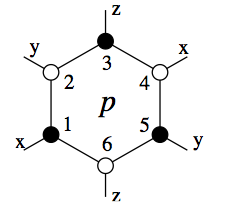
Figure 52: Pictorial rendition of the local symmetry of Eq. (223) associated with every hexagon Kitaev (2006).

Each of the six sites of the hexagon contributes only one component $\tau^{\gamma}$ of its pseudo-spin operator to the product $\hat{O}_{\varhexagon i}$, where $\gamma$ is either $x$, $y$ or $z$. Precisely which component of these three depends on the type of link that is not part of the hexagon – if on site $j$ the bond operator on the ”non-hexagon link” is of type $\tau^{\gamma}_{j}\tau^{\gamma}_{j+\bm{e}}$ (thus with $j\in\varhexagon i$ and $j+\bm{e}\not\in\varhexagon i$), the pseudo-spin component appearing in $\hat{O}_{\varhexagon i}$ is $\tau^{\gamma}_{j}$.

It can readily be verified that $\hat{O}_{\varhexagon i}$ commutes with any bond-operator $b_{jk}$ of Eq. (221) and consequently $[H_{\varhexagon}^{K},\hat{O}_{\varhexagon i}]=0$. These operators also mutually commute with one another: $[\hat{O}_{\varhexagon i},\hat{O}_{\varhexagon j}]=0$. Moreover the square of each such symmetry operator is one: $\hat{O}_{\varhexagon i}^{2}=1$. When it attains a non-trivial eigenvalue, i.e., $\hat{O}_{\varhexagon i}=-1$, the operator $\hat{O}_{\varhexagon i}$ is said to depict an anyonic charge or vorticity on hexagon $i$, for reasons which will become clear later.

From the above follows that the system is composed of $2^{N_{h}}$ sectors with $N_{h}=N/2$ being the number of hexagons. Each sector is specified by the the set of eigenvalues of the operators $\{\hat{O}_{\varhexagon i}\}$, where $i=1,...,N_{h}$: $|O_{\varhexagon 1}=\pm 1,O_{\varhexagon 2}=\pm 1,...,O_{\varhexagon N_{h}}\pm 1\rangle$.

The model has more symmetries. When the system is placed on a torus, $H_{\varhexagon}^{K}$ also has $d=1$ symmetries, using the classification of symmetries of Section VI.1. For any loop $C$ that spans the entire system the symmetry given by $\prod_{j\in C}\tau^{\gamma}_{j}$, where on each site $j$ the component $\gamma$ is determined by the character of one bond of site $j$ that is not on $C$ (i.e., the bond $\tau^{\gamma}_{j}\tau^{\gamma}_{j+\bm{e}}$ with $j\in C$ and $j+\bm{e}\not\in C$). When $C$ is for instance taken to be the zig-zag contour shown in Fig. 51 this symmetry is $\prod_{j\in C}\tau^{z}_{j}$, but actually any closed loop $C$ represents a symmetry.

X.3.2 Majorana Representation and Fermionization

The relations (i)-(iii) of the previous section define the bond algebra of $H_{\varhexagon}^{K}$ and it can readily be checked that they are also satisfied by the following substitution for the bonds in Eq.(221):

$$b_{jk}=2i\eta_{jk}c_{j}c_{k},$$ (224)

where the operators $c_{j}$ represent Majorana fermions, obeying the Majorana algebra as defined in Eq. (X.1.4) and $\eta_{jk}$ are Ising-type gauge links: a number that is either $+1$ or $-1$ on any given link $\langle jk\rangle$. With the ordering convention of bonds being that site $j$ always lies below site $k$, one has that exchanging sites $j$ and $k$ results in $\eta_{jk}=-\eta_{kj}$. The set $\{\eta_{jk}\}$ encompassing all bonds constitutes a sector of gauge links. In any given sector $\{\eta_{jk}\}$, the Hamiltonian of Eq.(222) is quadratic in the Majorana fermions $\{c_{i}\}$ and thus exactly solvable. Kitaev (2006); Nussinov & Ortiz (2009b)

The local ($d=0$) symmetries of Eq.(223) can be expressed in terms the bonds as

$$\hat{O}_{\varhexagon i}=\prod_{jk\in\varhexagon i}\eta_{jk}.$$ (225)

That is, each sector of fixed $\{\eta_{jk}\}$ is an eigenstate of the symmetry operators of Eq.(223) with an eigenvalue that is determined only by $\{\eta_{jk}\}$. In $\hat{O}_{\varhexagon i}$, as one multiplies $\eta_{jk}$ for all links $\langle jk\rangle$ that are in the hexagon $i$, one keeps the bond indices $j$ and $k$ ordered with the previously chosen convention of $j$ being below $k$.

The expression for $\hat{O}_{\varhexagon i}$ above highlights the similarity between the local gauge symmetries in this system and such general symmetry (and fluxes) elsewhere. For instance, in a lattice version of electromagnetism, Eq. (225) relates to an Aharonov Bohm like phase. In the current context, Eq. (225) relates to the Ising version of such a phase ($O_{\varhexagon i}=\pm 1$).

As each site belongs to three hexagons and each hexagon contains six sites, the number of hexagons is half the number of lattice sites ($N_{h}=N/2$). Thus to account for all eigenvalues of the operators $\{O_{\varhexagon i}\}$, it suffices to allow the $N/2$ degrees of freedom $\eta_{jk}$ on, for instance, all vertical bonds along ${\bm{e}}_{3}$ to attain a value of $\pm 1$ and to pin $\eta_{jk}$ on all other bonds (those along the ${\bm{e}}_{1}$ or ${\bm{e}}_{2}$ axis) to be 1. With this particular choice of the local gauge fields $\eta$, $\hat{O}_{\varhexagon i}$ in Eq.(225) reduces to the product of $\eta_{jk}$ on the two vertical links that belong to each hexagon $i$.

The dimensionality of the original Hilbert space of $N$ pseudo-spins is $2^{N}$. Thus in each of the $2^{N/2}$ sectors of $\eta_{jk}$, there is a remaining Hilbert space of size $2^{N/2}$ on which the Majorana fermions are defined. As explained in Sec. X.1.4, one representation for the $N$ Majorana fermions is in terms of $N/2$ spinless Dirac fermions. This may be explicitly done here by setting

$$c_{j}=d_{jk}+d_{jk}^{\dagger},$$

$$c_{k}=-i(d_{jk}-d_{jk}^{\dagger}),$$ (226)

with $d_{jk}$ a spinless Dirac Fermi operator on the vertical link $\langle jk\rangle$ (that is, $k=j+{\bm{e}}_{3}$) Chen & Nussinov (2008). The centers of the vertical links of the honeycomb lattice form a square lattice. It is therefore convenient to place the Fermi operators $d_{jk}$ and $d^{\dagger}_{jk}$) at the centers of the vertical links $\langle jk\rangle$) and henceforth denote these by $r$, leaving us with the operators $d_{r}^{\dagger}$, $d_{r}$ and the Ising degrees of freedom ${\eta_{r}}$. Denoting the unit vectors of the resulting square lattice by ${\bm{e}}_{x}$ and ${\bm{e}}_{y}$, the Kitaev-compass Hamiltonian reduces to

$$H_{\varhexagon}^{K}=J_{x}\sum_{r}(d_{r}^{\dagger}+d_{r})(d_{r+{\bm{e}}_{x}}^{\dagger}-d_{r+\hat{e}_{x}})$$

$$+J_{y}\sum_{r}(d_{r}^{\dagger}+d_{r})(d_{r+\hat{e}_{y}}^{\dagger}-d_{r+\hat{e}_{y}})$$

$$+J_{z}\sum_{r}\eta_{r}(2d_{r}^{\dagger}d_{r}-1).$$ (227)

The last term constitutes an analogue of a ”minimal coupling” term between gauge and matter degrees of freedom that is familiar from electromagnetism – in this specific case, an analogue of a coupling between the charge (or matter) density and an electrostatic type potential.

An advantage of the fermionization procedure employed above is that it does not require the use of elaborate non-local JW transformations. That the representation in terms of spinless fermions is $2^{N/2}$ dimensional can be checked by realizing that there are $N/2$ vertical links $\langle jk\rangle$ and the dimensionality of each spinless Fermion operator is two – the bond $\langle jk\rangle$ can be either occupied or un-occupied by a fermion.

Putting all of the pieces together, one sees that the problem of solving $H_{\varhexagon}^{K}$ has now been reduced to a problem involving solely fermions and Ising gauge degrees of freedom $\eta_{r}$, which at each site $r$ can only attain the value $\pm 1$. All excitations that appear in this system can be expressed in terms of the original spin variables ${\bf{\tau}}_{j}$ or, equivalently, in terms of fermions and Ising gauge fields.

The fusion rules that will appear both in this system and its non-Abelian extension that we will review in Sec. X.4.3 must relate to fermionic and Ising gauge type basic degrees of freedom.

X.3.3 Ground State of Fermionized Model

Within the ground state sector, for all hexagons all $\hat{O}_{\varhexagon i}=1$, or equivalently on the square lattice $\eta_{r}=1$ for all sites $r$. That the ground state must be vortex free is ensured by a corollary of a theorem due to Lieb, 1994 and has also been established numerically Kitaev (2006). In momentum space, the fermionized Hamiltonian of Eq.(227) assumes the form

$$H_{\varhexagon}^{K}=\sum_{\bm{q}}\epsilon_{q}d_{\bm{q}}^{\dagger}d_{\bm{q}}+i\frac{\Delta_{\bm{q}}}{2}\left(d_{\bm{q}}^{\dagger}d_{-\bm{q}}^{\dagger}+d_{\bm{q}}d_{-\bm{q}}\right),$$ (228)

where ${\bm{q}}=(q_{x},q_{y})$ and

$$\epsilon_{\bm{q}} = 2J_{z}-2J_{x}\cos q_{x}-2J_{y}\cos q_{y},$$

$$\Delta_{\bm{q}} = 2J_{x}\sin q_{x}+2J_{y}\sin q_{y}.$$ (229)

Interestingly, this Hamiltonian has the form of a p-wave BCS type Hamiltonian on the square lattice Chen & Nussinov (2008), which becomes explicit when the Hamiltonian is cast in the form of a Bogoliubov - De Gennes Hamiltonian

$$H_{\varhexagon}^{K}=\left(\begin{array}[]{cc}d_{\bm{q}}^{\dagger}&d_{-\bm{q}}\end{array}\right)H_{BdG}^{K}(\bm{q})\left(\begin{array}[]{c}d_{\bm{q}}\\ d_{-\bm{q}}^{\dagger}\end{array}\right),$$ (233)

where $H_{BdG}^{K}(\bm{q})$ is a $2\times 2$ matrix. It can be cast in the slightly more general form

$$H_{BdG}(\bm{q})=h_{\bm{q}}\sigma_{x}+\Delta_{\bm{q}}\sigma_{y}+\epsilon_{\bm{q}}\sigma_{z}={\bm{d}}({\bm{q}})\cdot{\bm{\sigma}},$$ (234)

where ${\bm{\sigma}}=(\sigma_{x},\sigma_{y},\sigma_{z})$ with Pauli matrices $\sigma_{x,y,z}$ and the last line defines the three-component vector ${\bm{d}}({\bm{q}})$. Here an extra coupling $h_{\bm{q}}$ has been introduced for future reference. This coupling is not present within the pure honeycomb Kitaev-compass model. Thus, $H_{BdG}^{K}=\lim_{h_{\bm{q}}\rightarrow 0}H_{BdG}(\bm{q})$.

In the Hamiltonian $H_{BdG}$, the vector ${\bm{d}}({\bm{q}})$ acts as a ”Zeeman field” applied to the ”spin” ${\bm{\sigma}}$ of a two-level system. All its eigenvalues come in pairs, corresponding to the energies

$$E_{\bm{q}}=\pm d({\bm{q}})=\pm|{\bm{d}}({\bm{q}})|=\pm\sqrt{{\bm{d}}({\bm{q}})\cdot{\bm{d}}({\bm{q}})}.$$ (235)

and eigenvectors

Diagonalizing the Hamiltonian by a Bogoliubov transformation

$$\gamma_{\bm{q}}=u_{\bm{q}}d_{\bm{q}}+v_{\bm{q}}d_{-\bm{q}}^{\dagger}$$ (236)

with $|u_{\bm{q}}|^{2}+|v_{\bm{q}}|^{2}=1$ and $|u_{\bm{q}}|^{2}=\frac{1}{2}\sqrt{1+\frac{\epsilon_{\bm{q}}}{E_{\bm{q}}^{2}}}$ gives the energy spectrum No effective chemical potential appears in this problem (i.e., $\mu=0$) so that within the ground state, all fermionic states of negative energy ($E_{q}<0$) are occupied while all states of positive energies are empty. The corresponding ground state wavefunction is

$$|g\rangle=\prod_{\bm{q}}(u_{\bm{q}}+v_{\bm{q}}d_{\bm{q}}^{\dagger}d_{-\bm{q}}^{\dagger})|0\rangle$$ (237)

Eigenvalues of the Bogoliubov - de Gennes come in pairs, at energies $\pm\epsilon$ with $\gamma_{-\epsilon}^{\dagger}=\gamma_{\epsilon}$, because of particle-hole symmetry. One fermion excitation eigenstate gives two solutions of the BdG equations. At $\epsilon=0$ is a Majorana fermion, as $\gamma_{0}^{\dagger}=\gamma_{0}$

In the vicinity of band extrema, the dispersions of Eq. (237) is of a parabolic when a gap appears between the two bands in the problem (i.e., $\min\{|E_{q}|\}>0$) and is linear near the zeros of $E_{q}$ when the system is gapless.

The ground state corresponds to a BCS condensate. In Chen & Nussinov (2008), real space ground state wave-functions $|\Psi_{0}\rangle$ were explicitly constructed in the original spin representation in closed forms that do not require any implicit projections. These Explicit ground states may be determined by writing the BCS wavefunction and undoing all of the steps employed here to map the spin problem onto a fermionic one. Time reversal invariance along with Kramers’ theorem ensures ground state degeneracy in systems with an odd number of spins. Explicit ground state wave-functions on a torus were constructed by Kells et al. (2009); these exhibit a four-fold topological degeneracy.

X.3.4 Gapless and Gapped Phases

Figure 53: Phase diagram of the honeycomb Kitaev-compass model. The triangle is the section of the positive octant $(J_{x},J_{y},J_{z})\geq 0$ by the plane $Jx+Jy+Jz=1$.The diagrams for the other octants are similar. Kitaev (2006)

To provide a better understanding of the spectrum, we focus on a particular set of couplings. At the symmetric system ($J_{x}=J_{y}=J_{z}$), the dispersion of Eq. (237) is, within the first Brillouin zone, zero at ${\bf q}^{(+)}\equiv{\bf K}_{1}/3+2{\bf K}_{2}/3,{\bf q}^{(-)}=2{\bf K}_{1}/3+{\bf K}_{2}/3$ where ${\bf K}_{1,2}$ denote the reciprocal lattice vectors along 1 and 2 directions Kitaev (2006) (and the equality holds modulo the addition of any reciprocal vectors). As the anisotropy of the coupling constants is increased (e.g., setting $|J_{z}|$ fixed and decreasing $|J_{x,y}|$), the two points ${\bf q}^{(}\pm)$ veer towards one another until they merge at the boundary between the gapped and gapless phases Kitaev (2006). Beyond this point, as $|J_{x,y}|$ are further decreased, and the system is in its gapped phase there are no real vectors ${\bf q}$ for which $E_{q}$ is zero.

In a similar fashion, the spectrum may be computed in other sectors. By looking at the algebra of the bonds appearing in the Hamiltonian, it is immediately clear that the spectrum is invariant under a change of sign of any of the exchange constants $J_{\alpha}\to-J_{\alpha}$. This, along with an overall global scale invariance of the gapless/gapfull parameter regions under a uniform scaling of all coupling parameters $J_{x,y,z}\to cJ_{x,y,z}$ with $c$ a constant enables us to delineate the boundaries of the gapless and gapped regions of the model. Such a phase diagram of the system is provided in Fig. 53 Kitaev (2006). The existence of transitions between these phases are “topological” and as such cannot be discerned by any standard local measurements. The inability of local measurements to discern between different phases underlies systems with topological order Kitaev (2003); Nussinov & Ortiz (2009c, a). When expressed in terms of the basic spin degrees of freedom, anyons involve extended non-local lines. Amongst other probes, an interesting signature of the topological transitions between the Abelian phases in Kitaev’s honeycomb model is afforded by quantum information theory measures, in particular the mutual information Cui et al. (2010).

The condition for a gapless phase is tantamount to the triangle inequality via Eqs. 229. This is so as the gapless phase implies $\epsilon_{q}=\Delta_{q}=0$ which in turn implies from Eqs. 229 (via the law of cosines) that one can view $q_{x}$ and $q_{y}$ as angles in the triangle formed by the sides $\{J_{x},J_{y},J_{z}\}$ Chen & Nussinov (2008). The relation between Kitaev’s honeycomb model and the $p-$ wave type pairing in Eqs. (227,228,229) was further elucidated in several insightful works, Yu & Wang (2008); Yu (2008).

X.3.5 Braiding Statistics

The Majorana fermion representation of Eq.(222) highlights another important property of this system- the braiding statistics formed by displacing one string of bonds around a closed loop. The product of bonds along any contour (open or closed) commutes with all other string products of the same form, including the symmetries $O_{h}$ of Eqs. (223,225). That is, for any contour $C$ drawn on the lattice, the operators

$$O_{C}=\prod_{ij\in C}b_{ij}$$ (238)

commute amongst themselves. For closed contours $C$, one has a sort of Stokes’ theorem. That is, the symmetries of Eq. 238 can be written as Chen & Nussinov (2008)

$$O_{C}=\prod_{h\in C}O_{h},$$ (239)

with the product taken over all hexagons $h$ that are enclosed by the loop $C$. The right-hand side of Eq.(239) corresponds to the total anyonic charge enclosed by $C$. If an odd number of anyons (hexagons $h$ for which $O_{h}=-1$) is circumscribed by $C$ then $O_{C}=-1$. This minus sign is the origin of the anyonic nature of the braiding operations in Kitaev’s model of Eq. 219, e.g., Chen & Nussinov (2008); Kells et al. (2008), in its gapped phase (known as the “A phase”). In the gapless phase of couplings of Kitaev’s model (“B phase”) of Eq. 219, the statistics of the vortices is ill defined. However, as will be elaborated on later, augmenting Eq. 219 by an additional external magnetic field term leads to the opening of a gap in the B phase. Within this gapped regime, the vortices exhibit well defined non-Abelian statistics.

An immediate corollary of the local ($d=0$) symmetries $O_{h}$ of Eqs. (223,225), is that, by Elitzur’s theorem, only correlation functions that are invariant under all of these symmetries may attain a non-zero expectation value at finite temperatures. Chen & Nussinov (2008) Thus, all non-zero correlation functions are composed of products of bonds (along closed or open contours) as in Eqs. (238,240). Similar considerations also apply at zero-temperature. [This is so as within the ground state $O_{h}=1$ for all $h$ while $O_{h}$, for a particular hexagon $h$, may be chosen to reverse the sign of a correlation function unless the correlation function is of the form of Eqs. (238,240.) Chen & Nussinov (2008)] These considerations generally lead to string and “brane” type correlation functions. [In fact, two-body and similar fermionic correlation functions of the local quadratic Fermi system defined by Eq. (227) become, upon the use of the JW transformation, such non-local string and brane type spin correlation functions Chen & Nussinov (2008).] While the above considerations revolve around symmetries of the spins alone, an earlier work illustrated, by the use of Majorana fermions, that all two-point correlation functions apart from those that form bonds vanish within the ground state and further related interesting consequences Baskaran et al. (2007).

In the gapped phase, these string correlation functions are exponentially damped in spatial distance between the endpoints of the string (with a similar behavior concerning dynamic correlations). Within the gapless phase, the string correlation functions decay algebraically in the distance.

X.3.6 Fermion Excitation and Translation

The fermionization procedure discussed above enables the construction of anyons out of string operators Chen & Nussinov (2008). A feature directly related to the symmetries of Eqs. (238,239) is that it is possible to create “fermionic” excitations alone sans anyons. One way to see this is by invoking symmetry and bond algebra arguments once again. Towards this end, one may consider the string product of bonds of the form of Eq. (238) yet now for an open contour $\Gamma$ (as opposed to the closed contour $C$). That is, we may define the operator

$$O_{\Gamma}=\prod_{ij\in\Gamma}b_{ij}$$ (240)

along an open contour $\Gamma$. For the purposes of what follows, let us label the end points of $\Gamma$ by $U$ and $V$. Unlike $O_{c}$ of Eq. (238), the operator of Eq. (240) is not a symmetry. That is, the operator $O_{\Gamma}$ serves as a trivial symmetry for all bonds $b_{kl}$ for which (1) $k,l\neq U$ or $V$ and/or (2) lie along $\Gamma:k,l\in\Gamma$. For all such bonds, $[b_{kl},O_{\Gamma}]=0$. The above includes all bonds $b_{kl}$ that have any number of sites along $\Gamma$ (i.e., 0,1, or 2) such that the bonds do not touch $\Gamma$ only at one point with that point being one of the endpoints $U$ or $V$. However, if $k=U$ or $V$ and $l\not\in\Gamma$ or vice versa (i.e., $l=U$ or $V$ and $k\not\in\Gamma$) then $b_{kl}$ will anti-commute with $O_{\Gamma}$:

$$\{O_{\Gamma},b_{kl}\}=0.$$ (241)

There are four such bonds $b_{kl}$. All other bonds commute with the operator of Eq. (240), $[O_{\Gamma},b_{mn}]=0$. As the exact solution that was outlined earlier [Eqs. (229, 237)] shows, the ground state sector of Kitaev’s model is not highly degenerate. As $O_{\Gamma}$ flips the energetic contributions of the four of the bonds $b_{kU}$ and $b_{Vl}$ that touch the endpoints $U$ and $V$, all of this suggests that the application of general $O_{\Gamma}$ (there is an exponentially large number of contours $\Gamma$) on a ground state cannot give back a ground state but rather must excite the system. The bonds at the end points of the contour $\Gamma$ have been modified (by a change of sign) as a result of the anticommutation relation of Eq. (241) and together the four disrupted bonds at the two endpoints $U$ and $V$ that do not lie along $\Gamma$ sum to yield a higher energy state. Thus, it is natural to associate defects created by the string operator of Eq. (240) at the endpoints $U$ and $V$ of the contour $\Gamma$. As seen from Eqs. (222, 240), the string operator $O_{\Gamma}$ involves only the Majorana fermions and not the anyons of Eqs. (223,225) and their composites (Eq. 239). Indeed, it is possible to verify that as each of the bonds of the lattice, $b_{ij}$ of Eqs. (221, 222) commutes with all anyonic charges $O_{h}$ of Eqs. (223,225), the operator of Eq.( 240) does not create [nor, in general, remove or displace) any anyons]:  $[O_{\Gamma},O_{h}]=1$. For a closed loop however, the closed string operator of Eqs. (238, 239) is a symmetry. The existence of general $d=1$ symmetry operators that are products of defect creation operators along loops Nussinov & Ortiz (2009c) has similar incarnations elsewhere (e.g., in Quantum Hall systems with the creation of quasi-particle/quasi-particle pairs). By creating defects and moving these defects along entire closed cycles, the defects annihilate and the system returns to its low energy (ground state) sector. Putting all of the pieces together, one sees that it is possible to have fermionic excitations (generated by Eq. (240)) alone. It is possible to express all of these results in terms of the fermions directly similar to Chen & Nussinov (2008).

When a fermion is transported around a closed loop that encircles a single Ising vortex (for which $O_{h}=-1$), we see that Eqs.(238, 239) reduce to an overall phase factor of $(-1)$. Thus, in such an instance the quantum state is multiplied by this overall phase factor Kitaev (2006).

X.3.7 Vortex Pair Creation and Translation

It is common to think about excitations formed by the application of single spin operators (i.e., by a rotation of a single spin) or by a product of two on the ground state. As pointed out by Dusuel et al. (2008), there are subtleties associated with simple interpretation of the action of these operations within the low energy sector. In what follows, we will focus on such an excitation via general symmetry and bond algebraic considerations. Towards this end, we consider a single vertical link $(ij)$. We define, similar to Kitaev (2006); Pachos (2006, 2007), the three operators $X=\tau_{i}^{x}\tau_{j}^{x}$, $Y=\tau_{i}^{x}\tau_{j}^{y}$, and $Z=\tau_{j}^{z}$. These operators are different from those Eq. (240) (including the case of a single two site bond). Each of these three operators anti-commutes with two bond operators. For instance, $Z$ anticommutes with the two bonds (other than $b_{ij}$) that have $j$ as one of their endpoints. Similarly, the operators $X$ and $Y$ each anti-commute with exactly two bonds. When acting on the ground state, the flipping operations incurred by any of the operators $X,Y$ or $Z$ may increase the system energy. It is furthermore readily verified that $Y$ and $Z$ may each flip the anyonic charges $O_{h}$ of two hexagonal plaquettes while $X$ flips the anyonic charges of all four hexagonal plaquettes that contain either the site $i$ or $j$ (or both). The flipping of any of the bonds generated by each of these three operators can be accounted for by inverting the sign of $\eta$ field along the corresponding link following Eq. 222. The three operators satisfy $S=1/2$ spin algebra:

$$\{X,Y\}=\{X,Z\}=\{Y,Z\}=0,$$

$$X^{2}=Y^{2}=Z^{2}=1,$$

$$XY=iZ,~{}YZ=iX,~{}ZX=iY.$$ (242)

It is natural to associate “particles” $X|\psi\rangle,Y|\psi\rangle,Z|\psi\rangle$ created by the application of the operators $X,Y$ or $Z$ on the ground state wavefunction. The last line of Eq. 242 generally suggests that a fusion of two particles into a third might be possible. This is indeed the case as it has been worked out in some detail in various approaches and limits (especially that of $J_{z}\gg J_{x,y}$ lying within the $A$ phases of the system, see Fig. 53 Kitaev (2006); Pachos (2007). In that limit, the energy of the the excitation $X|\psi\rangle$ is nearly equal to that of the sum of energies corresponding to $Y|\psi\rangle$ and $Z|\psi\rangle$.

As the anyonic charges of Eq.223 are symmetries, anyonic excitations are massive. That is, an anyonic excitation is stationary as it is an eigenstate of the Hamiltonian. As discussed in Dusuel et al. (2008), it is possible to create anyons without fermions by the combined use of one and three spin operations on the ground state. We now extend the discussion of the single bond operators above and present the general vortex translation (or anyon) operator. An approach related to ours, along with a detailed analysis of energies, is given in Kells et al. (2008). An insightful analysis is also provided in Dusuel et al. (2008). In order to analyze the Ising vortex translation operators, we introduce an operator that is identical to that of Eq. (240) apart from all important end point corrections that allow it to be expressed as $O_{\Gamma}$ multiplied by two operators corresponding to the two endpoints. Specifically, we consider an open contour $\Gamma$. For each non endpoint vertex $i\in\Gamma$, there is only a single neighbor $l$ that is not on $\Gamma$. For the two end points of $\Gamma$, ($i_{1}=U$ and $i_{2}=V$), there are two neighbors $l$ that do not lie on $\Gamma$. One may choose any of these neighbors for the two endpoints in what follows. (We will mark the chosen neighbors for the endpoints by $l_{1}$ and $l_{2}$ respectively.) We denote the direction of a ray parallel to the nearest neighbor link ($\langle il\rangle$) by $\gamma$ (that may be x, y, or z). We then construct the open contour operator

$${\cal{T}}_{\Gamma}=\prod_{i\in\Gamma}\tau_{i}^{\gamma}.$$ (243)

Eq. 243 is nearly of an identical form to Eq. 240 for all points non-boundary points $i$. However, in Eq. 240, the component of the boundary spin operators that appear in the string operator are such set equal to the two directions $\gamma_{1,2}=\langle i_{1,2}j_{1,2}\rangle$ with $j_{1,2}$ being the nearest neighbors of $i_{1,2}$ that lie on $\Gamma$ (i.e., “going backwards” away from the endpoints $i_{1,2}$). By contrast, in Eq. (243), the components of the spins at the two endpoints that appear in the string product are set by the two directions $\gamma=\langle i_{1,2}l_{1,2}\rangle$ (with $l_{1,2}$ not on $\Gamma$).

For the two hexagonal plaquettes $h^{*}=h_{1,2}$ that have a single vertex at one of the endpoints of $i_{1}$ or $i_{2}$ of $\Gamma$ and that furthermore include one of the vertices $l_{1}$ or $l_{2}$, we have that

$${\cal{T}}_{\Gamma}O_{h*}{\cal{T}}=-O_{h*}.$$ (244)

In eq. (244),$O_{h*}$ denotes the vortex charge of a plaquette $h*$ that lies at an endpoint of $\Gamma$.

Similar to the operator of Eq. (240), for all other plaquettes $h\neq h*$, we have that ${\cal{T}}_{\Gamma}O_{h}{\cal{T}}_{\Gamma}=O_{h}$ (with no change in the vortex charge).

It is readily verified that the operator ${\cal{T}}_{\Gamma}$, albeit flipping the sign of two bonds attached to the endpoints of $\Gamma$, does not alter the bond algebra of all bonds (all non- neighboring bonds commute, neighboring bonds anticommute, and the square of any bond is 1). The sole change triggered by the application of ${\cal{T}}_{\Gamma}$ is that two bond pre-factors $\eta$ are multiplied by a factor of (-1)). and correspondingly two vortex charges are flipped. Thus, the effect of ${\cal{T}}_{\Gamma}$ is to flip the sign of the two vortices at its endpoints.

If the system has a single vortex $O_{h_{1}}=-1$ at plaquette $h_{1}$ that has only one (endpoint) on $\Gamma$ and furthermore contains one of the two points $l_{1.2}$, then the application of ${\cal{T}}_{\Gamma}$ with the contour $\Gamma$ having a single point in the plaquette $h_{1}$ (the latter plaquette also containing the point $l_{1}$) as one of its endpoints will move the vortex to another plaquette $h_{2}$ that lies at the other end of the contour $\Gamma$ (and contains the point $l_{2}$).

That is, ${\cal{T}}_{\Gamma}$ is a vortex translation operator. If $\Gamma$ forms a complete closed contour $C$ along a toric cycle (when $h_{1}$ and $h_{2}$ are identified as the same point on the torus) then, similar to $O_{\Gamma}$ of Eq. (240), ${\cal{T}}_{\Gamma}$ veers towards the $d=1$ dimensional symmetry of Eq. (238). In the above, we established that the sole effect of ${\cal{T}}_{\Gamma}$ is to displace a vortex without influencing the system energy from any of the bonds that do not touch that endpoints of the contour $\Gamma$.

Although trivial, it may be noted that as pair permutations can be written in an SU(2) symmetric form as

$${\cal{P}}_{ij}=\frac{1}{2}(1+\bf{\tau}_{i}\cdot\bf{\tau}_{j})$$ (245)

and as any translation may be expressed as a product of pair permutations, general Majorana fermion and vortex translation operators may be expressed in an SU(2) symmetric form as a product of operators of the form of Eq. (245).

X.4 Kitaev-Compass Model – non-Abelian Phase

X.4.1 Definition of Extended Model

Kitaev’s model for a wide range of couplings corresponds, as earlier discussed (see Eq. (229, 237) to a gapless phase. This region is th so-called “B” phase of Kitaev’s model. It is only in the “corners” of the phase diagram of Fig. 53 ( the so-called “A” phase where the $\{J_{x},J_{y},J{z}\}$ differ substantially from one another and cannot form the sides of a triangle) that a gap opens up. As will be elaborated later on (sections (X.6, X.6.4, X.6.5), in the A phase, gapped Abelian anyons are present. Our focus in this section will be on the B phase where gapless excitations of Eq. (237) were found. By a modification of Kitaev’s honeycomb model, gapped non-Abelian excitations can arise. There are various ways in which such excitations can arise. For instance, these may be triggered by the geometry of the lattice (via, e.g., a decoration of the lattice wherein each vertex of the hexagonal lattice is replaced by a triangle Yao & Kivelson (2007)). In what follows, we review the original investigation of Kitaev (2006) in which a gapped phase with non-Abelian excitations originates from the application of an external magnetic field to a point $(J_{x},J_{y},J_{z})$ in the space of coupling constants for for which the system would have been gapless if no field were applied. [In this phase, the “B phase”, the couplings $J_{x},J_{y},$ and $J_{z}$ satisfy the triangle inequalities.] The B phase has made an appearance in studies quite removed from Kitaev’s model. Interestingly, in the quantum Hall arena, for half-filled Landau levels, this phase has also been suggested Barkeshli & McGreevy (2012) to appear to lie in the interface between a $\nu=1/2$ Moore-Read type state and a topological superconducting state as a periodic potential is tuned.

As we now review, such a field gives rise to an effective next nearest neighbor coupling between Majorana fermions. This additional hopping leads to a gapped spectrum with non-Abelian chiral modes. When a magnetic field ${\bf h}$ is applied along the $[111]$ direction, i..e., when Eq. 13 is augmented by a Zeeman coupling

$$H^{\prime}=H-\sum_{i}{\bf h}\cdot{\bf\tau}_{i},$$ (246)

a gap opens up in in the core region (B phase) of the phase diagram of Fig. 53. The (time reversal broken) phase that arises from the application of this field is very interesting.

In particular, non-Abelian anyons appear in the former gapless phase (which includes the symmetric point $J_{x}=J_{y}=J_{z}$). The Hamiltonian of Eq. 246 is not exactly solvable. It can, however, be treated perturbatively and (ignoring unimportant corrections) reduced to an exactly solvable system Kitaev (2006). That is, the magnetic field term in Eq. 246 gives rise (with $\kappa\sim h_{x}h_{y}h_{z}/J^{2}$ in the symmetric point $J_{x}=J_{y}=J_{z}=J$) to a (time reversal symmetry breaking) term of the form of Eq. (220) which we write here anew,

$$H_{h}=-\kappa\sum_{ijk}\tau_{i}^{x}\tau_{j}^{y}\tau_{k}^{z},$$ (247)

for all triplets of sites $(i,j,k)$ formed by the union of two bonds ($(ij)$ and $(jk)$) that impinge on site $j$. The product of the three spin operators of Eq. (247) can be expressed as a product of two neighboring bonds of Eqs. (221,224) by use of the relation $c_{j}^{2}=1/2$. For instance, for (oriented) links $(ij)$ and $(jk)$ along the x and z directions respectively (with $i_{z}<j_{z}$ abd $j_{z}<k_{z}$), the product of the bonds of Eq. (224) reads $b_{ij}b_{jk}=-2\eta_{ij}\eta_{jk}c_{i}c_{k}$. Eq. (247) is seen to reduce to a Majorana fermion bi-linear linking (all) next nearest neighbor sites. The Majorana fermion bi-linear ($c_{i}c_{k}$) resulting from the product of two bonds has a real prefactor ($-2\eta_{ij}\eta_{jk}$) as opposed to the imaginary prefactors that are associated with single nearest neighbor bonds in Eq. (224). This relative phase factor of $i$ reflects the time reversal symmetry breaking of the perturbation. Time reversal symmetry breaking also allows for the existence of chiral modes wherein fermionic modes may preferentially propagate in one (clockwise or anti-clockwise) direction. For any pair of next nearest neighbor sites $(ik)$ on the honeycomb lattice, there is a unique 3 site path (and two bond product) that leads to the bi-linear form $c_{i}c_{k}$. The quadratic character of these three-spin perturbations of Eq. (247)in the Majorana fermions (and similarly also in the fermions following, e.g., Eq. (X.3.2)) ensures that even when the system is augmented by these perturbations, the total Hamiltonian the final Hamiltonian

$$H_{K_{h};h}\equiv H_{K_{h}}+H_{h}$$ (248)

formed by the sum of Eqs. (13, 247) is still exactly solvable.

X.4.2 Solution of Extended Model

The solution to the problem is of a similar character to the one that earlier led to Eqs. (229, 237). As each spin product of the type $\sigma_{i}^{x}\sigma_{j}^{y}\sigma_{k}^{z}$ is given by a product of two bonds (each of which commutes with all of the symmetries of Eq. (223), it follows that the perturbation of Eq. (247) commutes with the operators $O_{h}$. As before, in any given sector one can employ the representation of Eqs. (221) with $\eta$ related to the flux via the condition of Eq.(225). All of the earlier steps taken in Eqs. (229- 228) can thus be exactly reproduced. However, unlike the nearest neighbor Hamiltonian that we we studied earlier in the absence of an applied external field $h$ (or an effective), the next nearest neighbor Fermi interactions lead new non-trivial results. In particular, the perturbation set non-zero ${\bf{h}}$ allows the earlier gapless phase in the absence of a field to become gapped and thus to support anyons which within this phase are non-Abelian Kitaev (2006). The spectrum of $H_{K_{h};h}$, in the vortex free sector ($O_{h}=1$ for all $h$) is then seen to be given by

$$E_{q}=\pm\sqrt{\epsilon_{q}^{2}+|\tilde{\Delta}_{q}|^{2}}$$ (249)

where the real p-wave type gap $\Delta_{q}$ Chen & Nussinov (2008) of Eq. (229) is now replaced by the complex

$$\tilde{\Delta}_{q}=\Delta_{q}+4i\kappa[\sin q_{1}-\sin q_{2}+\sin(q_{2}-q_{1})].$$ (250)

As can be seen by some simple analysis, the former gapless points ${\bf q}^{(\pm)}$ of Eq.(237) now acquire a gap when $\kappa\neq 0$. The p-wave type gap function Chen & Nussinov (2008) $\tilde{\Delta}$ now becomes complex. This suggests that the physics will essentially be the same as that for $``(p+ip)^{\prime\prime}$ superconductors Ivanov (2001). This is indeed the case as we will briefly reiterate later on. It is noteworthy that even when the Hamiltonian is time reversal invariant (as that of the system without perturbations- that of Eq. (13)), the ground states may spontaneously break time reversal. Indeed, by Kramers’ theorem, this must occur whenever the system is defined on a hexagonal lattice with an odd number of spins Chen & Nussinov (2008). In the B phase of Kitaev’s model wherein the gap was borne by the perturbation, the associated Chern number $\nu=\pm 1$ and the aforementioned non-trivial statistics Kitaev (2006) with non-Abelian topological anyons. We elaborate on these anyons and their features next.

X.4.3 Non-Abelian anyons and their properties

To conform with standard practice, we use $\sigma$ to denote a vortex (defined, similar, to the Abelian phase by having the plaquette product $O_{h}$ of Eqs. (223,225) be $(-1)$, $O_{h}=-1$) and $\epsilon$ is mark a fermionic mode. The fusion rules are then of the form

$$\epsilon\times\epsilon=I,$$

$$\sigma\times\epsilon=\sigma,$$

$$\sigma\times\sigma=I+\epsilon,$$ (251)

augmented by the trivial statement that the fusion of any particle with the identity operator leads back to that particle (as in, e.g., Eq. (213) for the Abelian anyons). As in the case of the Abelian anyons of Eqs. (211, 212), each particle is its own anti-particle. The non-trivial character of the non-Abelian anyons rears its head in the last line of Eq. 251. Two vortices ($\sigma$) may fuse in two different channels to either annihilate ($I$) each other or to form a fermion ($\epsilon$). The vortex operators of Eq. (223) have, as always, Ising eigenvalues $O_{h}=\pm 1$. Anyons that satisfy the relations of Eq. (251) are called “Ising anyons”. Unlike the case of Abelian anyons (e.g., Eqs. (211, 212)), fusing two different non-Abelian may lead to different outcomes (the vacuum ($I$) or an $\epsilon$ particle). In terms of Eq. (208), when choosing $a=b=\sigma$, there are two different anyonic outcomes for these non-Abelian anyons. In the limit of spatially infinitely distant vortices, the fermionic spectrum as adduced from the square lattice Hamiltonian of Eq. (214) with $\eta_{r}$ on the vertical links of original the honeycomb lattice set by the vortices $O_{h}$ of Eq. (225), exhibits a multitude of fermionic zero modes Lahitnen et al. (2008). Thus the hybrid of two well separated vortices ($\sigma$) may lead to a state in which the vortices annihilate to form the vacuum ($I$) or a “zero energy” fermionic state $(\epsilon$) This degeneracy is lifted once the vortices become close to one another wherein the fermionic modes $\epsilon$ attain a finite energy cost (or “mass”). Repeated applications of the last of Eqs. (251) rationalizes the $2^{n_{\sigma}/2-1}$ fold degeneracy that is present in a system of $n_{\sigma})$ (with this number being an even integer) well separated vortices Nayak & Wilczek (1996). In formal terms, the quantum dimension of the vortices $\sigma$ is $d_{\sigma}=\sqrt{2}$; the system degeneracy for $n_{\sigma}$ vortices scales $d_{\sigma}^{n_{\sigma}}$. Due to the unique outcome of all of the other fusion rules in Eq. (251), the quantum dimensions of $\epsilon$ and $I$ are $d_{\epsilon}=d_{I}=1$. The authors of Lahitnen et al. (2008) studied, in detail, the spectrum of Kitaev’s model and, in particular, the resulting spectrum for different vortex configurations in the non-Abelian phase. Lahtinen (2011) further illustrated how the fusion rules of Eq. (251) can be made evident by carefully studying the spectrum as the vortices were made to move towards one another with a distance that could be made continuous and examining the levels that appears in the limit of zero spatial separation between two vortices. The effective interactions between vortices that are held a finite distance apart (that trigger the aforementioned lifting of the topological degeneracy) exhibit an oscillatory character as a function of separation. The characteristic modulation length of these oscillations is set by the inverse Fermi momentum Lahtinen (2011) akin to that associated with vortices in $(p+ip)$ superconductors Cheng et al. (2009). Similar oscillations Baraban et al. (2009) appear in the Moore-Read Pfaffian wavefunction proposed for fractional Quantum Hall states Moore & Read (1991). We will review these and related properties in Section X.4.6.

Reflecting more on the relations of Eq. (251), one may consider a system with four well separated anyons $\sigma$ (denoted as $1,2,3,$ and $4$) which together fuse to form the vacuum $I$. In such an instance (similar to EPR type experiments Einstein et al. (1935)), the fusion outcome of any two $\sigma$ particles (e.g., $1$ and $2$) uniquely determines the particular fusion outcome of the other two $\sigma$ particles ($3$ and $4$). Namely, the outcome of the fusion of particles $a$ and $b$ is the same as that of fusing particles $3$ and $4$. As particles $1$ and $2$ can fuse in two different ways, there is a two dimensional space that is related to these four $\sigma$ particles. Focusing on the $\sigma$ particles $1$ and $2$ is, of course, artificial. One could have, e.g., focused on the basis set by the fusion result of particles $2$ and $3$. The matrix relating to such a change of basis is termed the “F-matrix”. More generally, in general systems, the matrix element $[F^{d}_{abc}]_{ef}$ is the amplitude that quasi-particles $a,b,$ and $c$ fuse and create quasi-particle $d$ in a specific fusion channel $e$. A schematic is shown in Fig. (54).

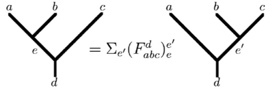
Figure 54: F-matrices relate the results of a fusion processes in which the order of events is changed. On the left, particles $a$ and $b$ are first fused together to form particle $e$; this particle is, in turn, then fused with particle $c$ to form particle $d$. The diagram on the right represents a process in which particles $b$ and $c$ are first fused to form a particle $e^{\prime}$ which is then fused with particle $a$ to form $d$. The outcomes of the two fusion processes are the same by the associativity property of fusion (Eq. (209)). The two orthonormal bases defined by $(e,c)$ and $(e^{\prime},c)$ are related to one another via the $F-$ matrix Wootton et al. (2008).

In the basis spanned by $(1,\psi)$, the model has the non-trivial $F$ matrix

$$F^{\sigma}_{\sigma\sigma\sigma}=\frac{1}{\sqrt{2}}\begin{pmatrix}1&1\\ 1&-1\\ \end{pmatrix},$$ (252)

and $F^{\sigma}_{\psi\sigma\psi}=F^{\psi}_{\sigma\psi\sigma}=-1$.

Braiding any two such particles with each other cannot change their fusion channel. This is so as their fusion channel or total charge may be determined along a distant path that circumscribes both particles. When two particles fuse in a definite channel, the outcome of revolving one of these particles around the other can only lead to a phase factor as diagrammatically depicted in Fig. (55). For the Ising anyons of Eq. (251), these phase factors are given by

$$R_{\sigma\sigma}^{I}=e^{-i\pi/8},~{}~{}~{}R_{\sigma\sigma}^{\epsilon}=e^{3\pi i/8}$$

$$R_{\epsilon\epsilon}^{I}=1,~{}~{}~{}R_{\sigma\epsilon}^{\sigma}=i.$$ (253)

In Eq. (253), $R^{c}_{ab}$ is the phase factor ratio between the (i) state that results by fusing two particles ($a$ and $b$) to a particle $c$ in a particular fusion channel of Eq.(208) following a counter-clockwise exchange of particles $a$ and $b$ to (ii) the fusion of particles $a$ and $b$ to form particle $c$ without such an exchange.

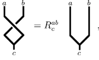
Figure 55: The R-matrix describes the effect of a counter-clockwise exchange of two particles on their fusion product. On the lefthand side, particles are exchanged in a counter-clockwise manner prior to their fusion. The resulting fusion product is related by the matrix element $R^{ab}_{c}$ to that without such a prior exchange Wootton et al. (2008).

Similarly, for the Abelian anyons of Eqs.(211, 212), which are pertinent to the Abelian phase of Kitaev’s model, the elements of the $R$ matrix are given by

$$R_{I}^{\epsilon\epsilon}=(R_{\epsilon}^{em})^{2}=-1,~{}~{}R_{I}^{ee}=R_{I}^{mm}=1.$$ (254)

We briefly comment on general topological quantum computing aspects Kitaev (2006); Nayak et al. (2008) which become most potent in systems with non-Abelian anyons such as those of Eq. (251). Within this general framework, an initialization proceeds by the creation of anyon pairs from the vacuum; this enables a knowledge of the particles and their fusion channels. Separating these anyons from one another gives rise to a degenerate manifold on which computations may be done. For the particular case of the vortex ($\sigma$) anyons of Eq. (251), as alluded to above, an $(n-1)$ bit space is generated from $(2n)$ far separated anyons. Braiding operations of anyons correspond to unitary gates. Measurements of the “calculation output” may be performed via the fusion of anyons and measuring energy to ascertain the fusion channel and/or by an interference experiment. Interference can be performed by creating a pair of anyons and, similar to the discussion in Section X.1 moving each of the members of the pair in different directions around another anyon along a $d=1$ loop. The final outcome following a recombination and fusion of the anyon pair members with each other depends on the state of measured anyon Kitaev (2006); Nayak et al. (2008).

As remarked earlier, fusion rules similar to those of Kitaev’s model appear also in $p-$ wave superconductors Ivanov (2001); Stone & Chung (2006). In the latter arena, $\epsilon$ represent Bogoliubov quasiparticles, $\sigma$ a vortex, and $I$ represents the Cooper pair ground state. The relation between the two systems might not be that surprising given the mapping employed here to relate Kitaev’s honeycomb model to a $p-$ wave type superconductor in the form of Eq. (214) which has a similar form yet with additional next nearest neighbor pairing and hoping terms once the interactions of Eq. (247) are included in the discussed form of Majorana fermion (and thus according to Eq. (X.3.2) also fermion) bi-linears. The non-Abelian nature of this theory may enable an anyonic quantum computer on a honeycomb model Kitaev (2006); Freedman et al. (2002). An edge mode is associated with each of the various excitations in Eq. (251).

Formally, the relations of Eq. 251 realize “SU(2)_k=2 algebra” (termed“level two SU(2)” algebra). This fancy name simply means that we may consider the basic objects to be usual (pseudo-)spins with the identity $I$ representing a trivial $S=0$ spin, particle $\sigma$ corresponding to a spin $S=1/2$, and $\epsilon$ corresponding to spin $S=1$. The fusion rules of Eq. 251 are then what is expected when adding two spins $S_{1}$ and $S_{2}$ for which there is the well known total spin decomposition

$$S_{1}\otimes S_{2}=|S_{1}-S_{2}|\oplus(|S_{1}-S_{2}|)+1)$$

$$\oplus....\oplus(S_{1}+S_{2}),$$ (255)

with the additional requirement that any total spin $S_{tot}>(k/2)$ on the righthand side of Eq. 255 is to be dropped (this is what the “level $k$” qualifier means). As in standard quantum mechanics, when we add two $S=1/2$ spins, there are two possible total total spin outcomes- i.e., $S_{tot}=0$ or $1$; this leads to the last line of Eq. 251. Similarly, when adding two $S=1$ spins (two $\epsilon$ particles) we have $S_{tot}=0,1,2$. However, as all but the $S_{tot}=0$ outcome have a total spin $S_{tot}>k/2$ with $k=2$, we have the single possible outcome on the first line of Eq. 251.

X.4.4 Berry, Wilczek-Zee phases & Relation to Anyonic Statistics

As is well known, when a system evolves adiabatically along a closed cycle in some general parameter space, it may accumulate a geometrical or “Berry” phase Berry (1984); Pancharatnam (1956). In quantum computation schemes, anyonic statistics is determined by the Berry phase associated with the motion of one anyon taken around another. Non-Abelian statistics may arise when unitary matrices $U_{ab}$ implementing different exchanges of different particles about one another do not commute. As alluded to earlier, in Eq. (207), in tese cases, ${\cal{T}}_{i}$ are non-commuting unitary matrices (of dimension $n={\cal{D}}_{U}\times{\cal{D}}_{U}$ with ${\cal{D}}_{U}>1$) acting on degenerate states. In the Hilbert space spanned by $n$ degenerate eigenstates, the Berry phase becomes a unitary matrix Wilczek & Zee (1984),

$$U={\cal{P}}\exp\{i\oint{\cal{A}}(\lambda)d\lambda\},$$ (256)

where ${\cal{P}}$ denotes a path-ordering in the parameter space $\lambda$ and

$${\cal{A}}_{\ell m}(\lambda)=i\langle\Phi^{\ell}(\lambda)|\frac{d}{d\lambda}\Phi^{m}(\lambda)\rangle,$$ (257)

with $1\leq\ell,m\leq n$. An adiabatic motion of fused vortices leads to Berry phases that tend to the braiding matrices associated with non-Abelian statistics as verified numerically by Bolukbasi & Valan (2011).

Berry phases may also be examined in the Abelian phase of Kitaev’s honeycomb model, e.g., Lian et al. (2011), and examine situations (other those of anyons) wherein the phase factors of Eqs.(256,257) may also be scalar (instead of more general matrices). Owing to the effective $d=1$ dimensional character of the generated excitations in Kitaev’s honeycomb model when spins are, e.g., rotated about the $z$ axis, the authors of Lian et al. (2011) sought to investigate the system under a “correlated rotation” corresponding to the evolution of the ground state wavefunction $|\Psi_{0}^{\prime}(\phi)\rangle=U(\phi)|\Psi_{0}\rangle$ where

$$U(\phi)=\exp[i\phi R],$$ (258)

$$R=\sum_{z-bonds}\tau^{z}_{j}\tau^{z}_{k}$$ (259)

with similar forms for $R$ associated with rotations about the $x$ or $y$ spin axes. The Berry phase is, in this case, set by $\Psi_{0}|R|\Psi_{0}\rangle$. We note this Berry phase of Lian et al. (2011) is simply the sum of the energies associated with the “z-bonds” of Kitaev’s honeycomb model. The authors of Lian et al. (2011) found that this phase factor (or bond energies) is, as is to be expected, non-analytic at the transition between the A and B phases. Specifically, Lian et al. (2011) examined the system behavior along the isotropic line $J_{x}=J_{y}$ as the coupling $J_{z}$ was varied. For the Berry phase of Eq. (259), second order derivatives of $\gamma$ were found to be divergent at the transition between the two phases. Such may be expected if the bond energies (and their differences as encountered in the 90^∘ compass model) play a role similar to that of an order parameter in a continuous second order transition. Numerically, oscillations in $\gamma$ were found in the “B phase” of Kitaev’s honeycomb model while those were absent in the gapped $A$ phase Lian et al. (2011).

X.4.5 General Features of (Majorana) Fermi Forms

As we reviewed above, in principle, Kitaev’s model can be solved (both without and with a perturbatively small magnetic field), within any vortex configuration ($\{O_{h}\}$) by mapping to a Fermi bi-linear. Specifically, we may find the exact spectrum of the Majorana Fermi bi-linear

$$H=\frac{i}{4}\sum_{jk}A_{jk}c_{j}c_{k}$$ (260)

with the fermionic substitution of Eq. (X.3.2) where $\{O_{h}\}$ determine $\eta_{jk}$ by Eq. (225) where we set $\eta_{jk}$ on all vertical links to be $(+1)$ in any sector of the topological charges $\{O{h}\}$. Such general (essentially free fermion systems in the diagonal basis) systems are completely characterized by their band structures $E_{q}$. The exact ground states of this system corresponds to occupying all states below the Fermi energy (whose value is $\mu(T=0)=\epsilon_{F}=0$). The pair correlator between any two single particle fermionic states is one if both states are occupied (have negative energy) and zero otherwise. Topological features such as Chern numbers are associated with the projection operators to the negative energy states for these dispersions in momentum space. In his seminal work, Kitaev Kitaev (2006) analyzed the resulting Fermi surface topology using these.

As noted in section X.4, an explicit diagonalization of the general bi-linear of Eq. 260 Kitaev (2006); Lahitnen et al. (2008) as it pertains to Kitaev’s honeycomb model in the presence of the next nearest neighbor fermion interactions stemming from the perturbation of Eq. (247) reveals that the system features a spectrum containing a continuum of positive and negative energy states with a gap in between them with, as in many other systems (such as integer quantum Hall systems and polyacetelyne chains), discrete additional mid-gap (or fermionic zero mode) states whose energy vanishes for some momenta. In real space, these zero energy states correspond to states that are localized near the boundary. As a function of momentum, the energies of the states changes from positive to negative to the projection operators onto the negative energy states (that are all occupied at zero temperature) changes abruptly at these wave-vectors. These discontinuities are topologically distinguished by the so-called Chern number alluded to earlier. The general form of the bi-linear of Eq. 260 enables a simple and exact form for the spectral Chern number $\nu$ Kitaev (2006). A physical consequence of this topological invariant is that energy spectra corresponding to different different Chern numbers cannot be adiabatically connected- a quantum phase transition must intervene as $\nu$ is changed.

Similar to electronic systems (with a chemical potential $\mu=0$), in our discussion of the single particle spectra of Eq. (237), within the ground state $|\psi\rangle$ all single particle fermionic state that are of negative energy are occupied and those with energy $E_{q}>\mu=0$ are unoccupied. The projection operator to the negative energy states $E_{q}<0$ can be expressed in the original Majorana Fermi basis as

$$P_{jk}=\langle\psi|c_{k}c_{j}|\psi\rangle.$$ (261)

Formally, this projection depends the wave-vector parameter index and thus defines a (one-dimensional) vector bundle which corresponds to a non-trivial Chern number. Specifically,

$$\nu=\frac{1}{2\pi i}\int dq_{x}dq_{y}Tr\Big{[}P(\vec{q})\Big{(}\frac{\partial P}{\partial q_{x}}\frac{\partial P}{\partial q_{y}}-\frac{\partial P}{\partial q_{y}}\frac{\partial P}{\partial q_{x}}\Big{)}\Big{]}.$$ (262)

As briefly noted in section X.2.1, the Chern number ($\nu$) characterizes the difference between the number of different “left” and “right” movers along the boundary of the system (if such a system occupies a half plane) Kitaev (2006). We will elaborate and briefly re-iterate some aspects concerning Chern numbers below. The Chern number assumes integer values. The values of the Chern numbers aid in identifying different phases in Kitaev’s honeycomb model. Even values of $\nu$ correspond to Abelian phases whereas odd Chern numbers appear in non-Abelian phases. A non-zero value of the Chern number, $\nu\neq 0$, indicates a chirality.

The edge modes carry thermal energy and thus as in Quantum Hall systems Cappelli et al. (2002) (where the Chern number is equal to the filling fraction), the Chern number can be adduced by thermal transport measurements Kitaev (2006). Specifically, at a temperature $T$, the edge energy current is given by

$$J=\frac{\pi\nu}{24}T^{2}.$$ (263)

The physics of the Fermi gas (that of decoupled Fermi modes) largely underlies the results that we presented for the Kitaev model. In this case, when considering the edge current, the physics is that of decoupled fermi modes on the system boundary- i.e., that of a one dimensional fermionic system Kitaev (2006). These considerations appear elsewhere and are very powerful.

For multi-band systems, we can project the system onto each band separately and compute the Chern number that corresponds to each such band. The total Chern number associated with the negative bands is opposite in sign and equal in magnitude to the total Chern number associated with the positive energy bands.

Whenever $\nu=\pm 1$, every vortex must carry an unpaired Majorana mode. Unfortunately, translational symmetry is broken by vortices ($O_{h}\neq 1$) and the system in a general sector is diagonalized in a sector other than that of momentum space. Rather, we need to diagonalize another general structural matrix defined by $A$. In the general case, the Chern number is defined modulu 16. This relates to a topological phase of the vortices given by $\exp[2\pi i\nu/16]$. Only three of these phases are of relevance (the Abelian case of $\nu=0$ and the non-Abelian phase with $\nu=\pm 1$ that is induced by an external magnetic field. In particular, when $\nu$ is odd, it is not possible to define a structural matrix in the presence of vortices $O_{h}=-1$. A Chern number of $\nu=0$ corresponds to the corners of the phase diagram of Fig. 53 in the Abelian phase of the model where the triangle inequality relating $J_{x},J_{y}$ and $J_{z}$ cannot be satisfied.

Similar to the general discussion of subsection X.1, we can define magnetic and electrical topological charges here. In this case, these correspond to the anyon charges $O_{h}=-1$ on alternating horizontal rows of hexagonal plaquettes of the honeycomb lattice. It is possible to change a magnetic vortex into an electrical one by the creation/absorption of a fermion $\epsilon$. Denoting by $m$ and $e$ magnetic and electrical charges and by $I$ the vacuum ($O_{h}=1$), there are, in this (Abelian) phase fusion rules identical to Eqs. (211, 212).

X.4.6 Ground States Properties in Vortex-full Sectors

As briefly alluded to earlier, the fusion rules of Eq. (251) and their consequences may be understood by examining the system in the presence of vortices. The calculations within the vortex full sectors proceed along the lines identical of subsections X.3,X.4. In the bare Kitaev model Hamiltonian of Eq. (13) [which may be augmented by the perturbation of Eq. (220)], we set $\eta_{r}$ on the vertical links to be such that the vorticity of Eq. (225) satisfies $O_{h}=\eta_{r}\eta_{r^{\prime}}$ where $\eta_{r}$ and $\eta_{r}^{\prime}$ denote the Ising degrees of freedom on the two vertical links of the plaquette $h$ of the original hexagonal lattice. As we reviewed earlier, the resulting Fermi form [also in the presence of the perturbation of Eq (247)] is a bi-linear with on-site and nearest neighbor (resulting from the Hamiltonian of Eq. (13)) and next nearest neighbor (resulting from Eq. (247) (hopping and pairing) terms on the square lattice which may be exactly solved. The Fermi spectrum may, specifically, be exactly determined within each of the $2^{N/2}$ sectors (i.e., values $O_{h}=\pm 1$ on each of the $N_{h}=N/2$ hexagons). Practically, it is possible to exactly (numerically) solve for the spectrum of the system in simple insightful sectors. These include a system with a single pair of vortices, a superlattice of uniformly spaced vortices, and other intermediate and other related regimes. General trends are seen and we elaborate on those below.

Vortex pairs: oscillations, midgap states, and fusion: We first briefly review several key aspects of a system with a single pair of vortices Lahtinen (2011) in the presence of a field (Eq. (247)). When two non-Abelian anyons are held at a finite distance $d_{s}$ apart and the system eigenstates are computed, it is found that in addition to the gapped fermionic modes there appear two additional modes. The continuous particle-hole symmetric spectrum is augmented by an additional pair of energies Lahtinen (2011)

$$\pm\Upsilon^{d_{s}}=\pm\Delta_{f}\cos(2\pi d_{s}/\lambda)e^{-d_{s}/\xi}.$$ (264)

These new vortex states of low energy states (i.e., low $\Upsilon$) augment the continuous bands of higher energy Fermi bands (of energies $\pm E$,   $E>\Upsilon^{d_{s}}$) that appear here similarly to the case of the vortex free lattice (Eq. (249)). As the separation $d_{s}\to\infty$, these additional modes veer towards zero energy and become midgap states between the positive and negative fermionic energy bands $\pm E_{q}$ of the vortex free system. By continuously changing the separation $d_{s}$ to zero, Lahtinen (2011) elegantly illustrated how the Majorana Fermi fusion mode $\epsilon$ of Eq. (251) is explicitly realized. The gap $\Delta_{f}$ of Eq. (264) sets the minimal energy of these fermionic excitations. As is manifest in Eq. (264), at finite separation $d_{S}$, the virtual exchange of these Fermi fusion modes lifts the degeneracy. The size of the gap $\Delta_{f}$ is an effective confining barrier height that needs to be surmounted for the fermionic fusion modes to become delocalized Lahtinen (2011). Thus, the picture that emerges at finite inter-vortex separation $d_{s}$ is that of Majorana fusion modes that are bound to the vortices. The modulation length $\lambda$ in Eq. (264) is set by the reciprocal of the difference between the wave vectors (${\bf{q}}^{(\pm)}$) that minimize the energy of Eq. (249), Lahtinen (2011)

$$\lambda\simeq\frac{2\pi}{|{\bf{q}}^{(+)}-{\bf{q}}^{(-)}|}.$$ (265)

Similar oscillatory decay appears in other systems that harbor Majorana excitations Cheng et al. (2009); Baraban et al. (2009). More broadly, effective interactions on non-uniform sign such as those of Eq. (264) also appear in numerous classical systems including RKKY interactions in spin glasses, theories of structural glasses, and other systems with competing interactions Yosida (1957); Kasuya (1956); Ruderman & Kittel (1954); Chakrabarty & Nussinov (2011); Nussinov (2004); Nussinov et al. (1999); Tarjus et al. (2005). In a many particle system, such an oscillatory character of the effective pair interactions may reflect frustration and consequently lead to multiple inhomogeneous states and viable slow dynamics.

Multiple vortices and vortex lattices The understanding of the single vortex pair problem and the bound states that form therein allows a qualitative understanding of the $n$ vortex pair problem. For well separated vortices, there is a $2^{n}$ fold degeneracy of the ground state. Majorana fermion modes may tunnel and realize the mode $\epsilon$ associated with the fusion channel of Eq. (251). Vortices partially bind Majorana modes and lead to a lifting of the degeneracy when the inter-vortex separation is finite and lead to a localization of the Majorana zero modes.

As the number of vortex pairs $n$ is increased yet is far smaller that the number of sites on the lattice, additional (fusion borne) midgap states appear that are well separated from the continuum of modes at positive and negative energies Lahtinen (2011); Lahtinen et al. (2011). The wave-functions corresponding to these midgap states preferentially have their spatial support localized on the vortices. By contrast, the real space wave-functions corresponding to the fermionic states at the continuum of energies $\pm E$ are uniformly delocalized on the lattice. We remark that the physics that emerges as the number of vortices is increased is qualitatively similar to that in other systems (e.g., doped semiconductors (or superconductors)) with an increased number of dopants that modify the local hopping (and pairing) amplitudes. In lattices with a dense set of vortices, the new Majorana states that appear (vis a vis those in the vortex free problem) may lead continuous bands. These new modes may overlap with those borne out of the continuous modes Lahtinen (2011); Lahtinen et al. (2011). Interactions may hybridize low-energy bands from the multitude of these new fusion borne modes. We remark that when the vortices are arranged in a periodic lattice, the fermionic system is periodic and should exhibit multiple momentum space bands (which may be regarded as a hybridization of the individual fusion type modes) associated with an enlarged unit cell (set by the period of the vortex lattice). The emergence and evolution of these new bands as a function of vortex lattice spacing was carefully studied in Lahtinen et al. (2011). It is possible to account for the Chern number and other characteristics of the different phases as seeing from as originating from the sum of two different contributions: (i) continuum Fermi bands and the (ii) new Majorana modes that appear in the vortex lattice and may be approximately viewed as hopping between the vortices (to which they are preferentially bound)- this may be emulated by a kinetic term with complex short range hopping amplitudes between Majorana fermions on the vortex lattice sites Lahtinen et al. (2011). The extreme case of the fully dense vortex lattice (i.e., a vortex on every plaquette) was investigated in Lahtinen & Pachos (2010). The Fermi surface associated with this theory undergoes a quantum phase transition from the usual non-Abelian phase (with Chern number $\nu=-1$) with a single pair of continuous fermionic modes to an Abelian chiral phase (with Chern number $\nu=-2$) that supports the above mentioned new additional bands Kitaev (2006); Lahtinen & Pachos (2010). As re-iterated above, these new bands in vortex lattices (including the maximal dense vortex lattice) may be seen as brought about by the merger of the Majorana fusion modes that appear in the dilute vortex pair problem.

X.5 Classical Ground States & Dimer Coverings

Similar to the compass models that we studied in earlier sections, fluctuations (both zero-point quantum fluctuations as well as (classical) thermal fluctuations) can stabilize order in Kitaev’s honeycomb model.

Following Baskaran et al. (2008) we review features of the large $S$ rendition of the Kitaev model. Similar to the large $S$ extension of the 120^∘ and 90^∘ compass models Nussinov et al. (2004); Biskup et al. (2005) in Eq. 140 and the discussion in Section VIII, we may replace each spin operator in Eq. 13 by a classical vector to obtain the classical ($S\to\infty$) limit. We may similarly define the Kitaev model in this fashion for arbitrary $S$ Baskaran et al. (2008).

Building on the general discussion of classical ground states in Section(VIII), we note that employing the same counting arguments that we invoked earlier shows that there are, on the honeycomb lattice, $(3N/2)$ independent conditions stemming from Eq. (149). On the other hand, $N$ classical three component pseudo-spins have $(2N)$ degree of freedom (i.e., two angles specify the orientation of a pseudo-spin on the unit sphere for each of the $N$ pseudo-spins). Thus, by naive counting there remain $(N/2)$ redundant degrees of freedom suggesting a local emergent gauge symmetry. (This number is equal to the number of hexagons: $N_{h}=N/2$.)

The system has a rich structure at its symmetric point: $J_{x}=J_{y}=J_{z}$ in the classical rendition of Eq. 13. Similar to the classical compass models discussed in Section VIII Nussinov et al. (2004); Biskup et al. (2005) there is an emergent continuous symmetry in the ground state sector. To elucidate these, we note that the honeycomb is bipartite– it is possible to partition of the sites of the lattice into two sublattices (say, A and B) such that points in the A sublattices have all of their neighbors in the B sublattice (and vice versa). With this in mind, we note that we may generate ground state if we orient all of the spins in the A sublattice along the same direction and then orienting all of the spins on the B sublattice along the opposite direction. Baskaran et al. (2008)

The above set of ground states harboring emergent symmetries is augmented by a discrete set of states. Baskaran et al. (2008) In these, we set two spins at the endpoints of a link to be anti-parallel to each other and be oriented along the spatial direction of the link. For instance, we may set the two spins along a link that is parallel to the spatial $x$ direction to be anti-parallel to each other and point along the $\hat{e}_{x}$ and $(-\hat{e}_{x}$) directions. These ground states thus reduce to dimer coverings and are of a similar form to the suggested low energy states that we encountered in the 120^∘ model on the honeycomb lattice Nasu et al. (2008). [See section IX.5.2.] The problem of enumerating these discrete states may be mapped onto that of examining dimer coverings of the lattice. That is, we may ask in how many ways we can place dimers on the links of the lattice. Once a dimer is placed, we orient the spins at the endpoints to be parallel/anti-parallel to the spatial direction of the dimer. The number of dimer coverings of the honeycomb lattice with N sites is equal to

$${\cal{N}}_{dimer}\simeq 1.175^{N}.$$ (266)

If we take into account the possibility of placing the spins parallel to anti-parallel to the spatial direction of the link, we find that the total number of discrete classical ground states is

$${\cal{N}}_{discrete~{}classical}={\cal{N}}_{dimer}\times 2^{N/2}\simeq 1.662^{N}.$$ (267)

X.5.1 Symmetries of Spin-S Systems

For general (pseudo-spin) $S$ renditions of Kitaev’s honeycomb model, the conserved $S=1/2$ quantities of Eq. (223) are replaced by Baskaran et al. (2008)

$$O_{h}=\prod_{j=1}^{6}e^{i\pi T_{j}^{a_{j}}}$$ (268)

where $a_{j}$ denotes the direction of an outward “spoke” at site $j$ that is normal to the hexagon $h$ and $T_{j}$ is the $j$th pseudo-spin compoent. Similar to the (pseudo-)spin one half case, generalizations of Eqs. (238,239) associated with any closed contour $\Gamma$ are conserved quantities (symmetries of the model). Rather explicitly, these are Baskaran et al. (2008)

$$O_{\Gamma}=\prod_{j\in\Gamma}e^{i\pi T_{j}^{a_{j}}}.$$ (269)

X.5.2 Spin-wave Expansion

The degeneracy of the classical ground states described in Section X.5 is partially lifted by quantum fluctuations as manifest in $(1/S)$ corrections to the energy. For a one-dimensional version of the general spin S Kitaev model, it was found that incorporating ($1/S)$ corrections made the discrete set of classical ground states lower in energy than their continuous counterparts. Baskaran et al. (2008).

With each dimer covering that represents a discrete classical ground state, there is an associated set of self avoiding walks. These walks are formed by walks such that no link that lies on the self avoiding walk is a dimer that represents the spin orientation in the ground state.

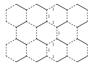
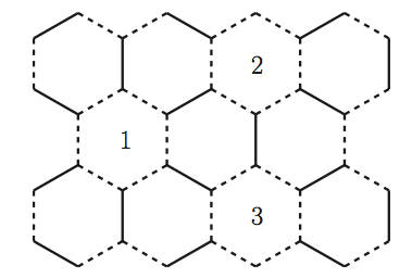
Figure 56: Mappings between dimer configurations (solid lines) and self-avoiding random walks (dashed lines), see text. Baskaran et al. (2008).

X.5.3 Quantum Ground States and Dimer Coverings

In a very interesting work, Nash & O’Connor (2009) illustrated that, in the absence of vortices, the zero temperature phases of the (pseudo-spin 1/2) Kitaev model on general lattices are in a one to one correspondence with those of classical dimer coverings Fisher (1966); Friedland & Gurvits (2008) on the same lattice. This result may be viewed as complimentary to the results of Baskaran et al. (2008) as they pertain to the classical, large $S$, Kitaev model on the honeycomb lattice. [See, subsection X.5.] On sufficiently complicated lattice realizations of the pseudo-spin 1/2 Kitaev mode wherein the couplings are orientation dependent and furthermore are varied to become spatially non-uniform e.g., a honeycomb lattice with an eighteen site basic periodic block, a new gapped (“C”) phase was seen to emerge inside the “B” phase.

Viable lower energy states for general pseudo-spin $S$ were provided by Chandra et al. (2010). These are constructed out of superpositions of the product states. The idea underlying these states is elegant and we briefly review it below within the general approach employed in this review. The honeycomb lattice can be decomposed into disjoint hexagons and a set of links between these on which the different hexagons interact: $\sum_{hex}H_{hex}+\sum_{int}H_{int}$ Chandra et al. (2010). The interactions around a hexagonal plaquette (those in $H_{hex}$) satisfy, obviously, the bond algebra earlier discussed Eq. (221). For a single hexagon, the algebra is that of bonds around a six site chain that anticommute if they are nearest neighbors, commute otherwise, and always square to 1. Thus, by a trivial change of basis , all bonds may be made to be of the xx or yy type. The resulting six site Hamiltonian is then

$$H_{hex}=-J(T_{1}^{x}T_{2}^{x}+T_{2}^{y}T_{3}^{y}+T_{3}^{x}T_{4}^{x}$$

$$+T_{4}^{y}T_{5}^{y}+T_{5}^{x}T_{6}^{x}+T_{6}^{y}T_{1}^{y}).$$ (270)

The classical ground state of this Hamiltonian would be the uniform state wherein all spins are polarized along some direction $\phi$ in the xy plane. Chandra et al. (2010) then consider the quantum product state analogue of the corresponding coherent states at the six sites $|\phi...\phi\rangle=|\phi\rangle_{1}\otimes...|\phi\rangle_{6}$. The spin state at site $i$ can be expressed as $|\phi\rangle_{j}=(\frac{1}{2})^{S}\exp[i\phi T_{j}^{-}]|T_{z}=S\rangle_{j}$ with $T_{j}^{-}=(T_{j}^{x}-iT_{j}^{y})$. A candidate product state over the entire system of all hexagons is then suggested to be $\otimes|\psi\rangle_{h}$ with, at each hexagon $h$,

$$|\psi_{h}\rangle=\frac{1}{2\pi}\int_{0}^{2\pi}e^{-6S\phi i}|\phi\phi...\phi\rangle.$$ (271)

Computing the energy of this trial state with the full Hamiltonian (involving also the interactions between hexagons) leads to reasonable results. This procedure and be improved in a variety of ways (e.g., employing exact quantum ground states on large units and optimizing with respect to the interactions between those units).

X.5.4 Bounds on Ground State Energies

In an elegant work Chandra et al. (2010), exact bounds on the ground state energies of the pseudo-spin $S$ rendition of Kitaev’s honeycomb model were provided for the system at its symmetric point ($J_{x}=J_{y}=J_{z}$) in the absence of perturbations. A lower bound for the energy was obtained by determining the minimal possible energy for a small unit of a site on one sublattice with all of its (three) nearest neighbors (on the other sublattice); the Hamiltonian can be written as a sum of the interactions found in these chosen units (or bonds). Such a decomposition has afforded bounds on ground state energies of, e.g., bipartite quantum antiferromagnets Anderson (1951); Carlson et al. (2008). Upper bounds on the ground state energy were obtained via a variational argument using a product of wave-functions on two-sites (extensions include larger size units as discussed in subsection X.5.3 above). Putting all of the pieces together, the ground state energy was found to satisfy inequalities for all $S$ systems. In the $S\to\infty$ limit, these read

$$-\frac{1}{2}+\frac{1}{4S}\leq\frac{E_{0}}{JN}\leq-\frac{1}{2}+0.374\frac{1}{S}$$ (272)

A related yet slightly different lower upper quadratic estimate was obtained by Baskaran et al. (2008) wherein the $1/S$ correction in the bound of Eq. (272) was replaced by $(0.289/S)$.

X.5.5 Classical Order out of Disorder

The authors of Chandra et al. (2010) report that unlike most other compass models, Kitaev’s model in its classical version does not exhibit a finite temperature order out of disorder effect and that quantum fluctuations are required to attain order. This conclusion relates to the general character of quantum and classical order out of disorder mechanisms, see section VIII.1.

X.6 Toric Code Model

X.6.1 Relation between Kitaev Compass & Toric Code Models

In its low energy sector, the gapped phase of Kitaev’s model of Eq. 13 is adiabatically connected to Kitaev’s toric code model which we will study in subsection X.6.2. In the limit of extreme anisotropy (e.g., $|J_{z}|\gg|J_{x,y}|$), Kitaev’s honeycomb model of Eq. (13) reduces to the Toric code model of Eqs. (273,274) Kitaev (2006). In this limit, all of the bonds along the $z$ direction are strongly correlated and effectively the strong correlated spins along the two sides of a given $z$ bond (a “vertical dimer”) may be replaced by one spin. Geometrically, the replacement of vertical dimers of the honeycomb lattice by singlet sites is similar to what we have earlier encountered in the solution of Kitaev’s honeycomb model by replacing it by a fermionic system on a square lattice [Eq.(X.3.2)]. Analogously, the resulting geometry in the case of extreme anisotropy (e.g., $|J_{z}|\gg|J_{x,y}|$) is that of the square lattice of the Kitaev Toric code model on the square lattice which we will next discuss. Within the low energy subspace of Kitaev’s honeycomb model, the Toric model below results from the lowest non-trivial order (a fourth order contribution) in the perturbative expansion in $(J_{x,y}/J_{z})$ about the $J_{z}\to\infty$ limit of decoupled vertical dimers. When Kitaev’s honeycomb model is not projected onto the low energy subspace (that of no fermionic excitations), there are additional terms that augment the correspondence to Kitaev’s toric code model Dusuel et al. (2008). As we will discuss in the section X.6.2, Kitaev’s toric code model exhibits an Abelian (“$Z_{2}\times Z_{2}$ type”) statistics identical to that of Eqs. (211,212). As the gapped phase of Kitaev’s honeycomb model is adiabatically linked to the toric code model, the honeycomb model also exhibits, everywhere within its gapped phase, this $Z_{2}\times Z_{2}$ symmetry.

X.6.2 Kitaev’s Toric Code model: Definition, Symmetries & Ground States

Kitaev’s Toric code model Kitaev (2003) in $D=2$ spatial dimensions is defined on a square lattice with $L\times L=N_{s}$ sites, where on each link $\langle ij\rangle$ there is a $S=1/2$ degree of freedom, see Fig. 51(B). The Hamiltonian of this model is given by

$$H_{K}=-\sum_{s}A_{s}-\sum_{p}B_{p}\;,$$ (273)

with the operators

$$A_{s}=\prod_{\langle ij\rangle\in{\sf star}(s)}\sigma_{ij}^{x},\hskip 28.45274ptB_{p}=\prod_{\langle ij\rangle\in{\sf plaquette}(p)}\sigma_{ij}^{z},$$ (274)

and $\sigma_{ij}^{\kappa}$ ($\kappa=x,y,z$) representing Pauli matrices. $B_{p}$ and $A_{s}$ describe the plaquette (or face) and star (or vertex) operators, respectively, with ($\forall s,s^{\prime},p,p^{\prime}$)

$$[A_{s},A_{s^{\prime}}]=[B_{p},B_{p^{\prime}}]=[A_{s},B_{p}]=0,$$ (275)

generating an Abelian group which is known as the code’s stabilizer Kitaev (2003), and the two $d=1$ (Ising type (${\mathbb{Z}}_{2}$)) symmetries are given by Kitaev (2003)

$$Z_{1,2}=\prod_{\langle ij\rangle\in C_{1,2}}\sigma_{ij}^{z},\hskip 28.45274ptX_{1,2}=\prod_{\langle ij\rangle\in C^{\prime}_{1,2}}\sigma^{x}_{ij},$$

$$\{X_{\mu},Z_{\mu}\}=0\ ,\hskip 14.22636pt[X_{\mu},Z_{\nu}]=0\ ,\hskip 14.22636pt\ \mu\neq\nu,$$ (276)

where $C_{1}(C_{2}^{\prime})$ are horizontal and $C_{2}(C_{1}^{\prime})$ vertical closed contours [i.e., loops on the lattice (dual lattice)] that span an entire cycle of the torus. The non-commutativity of the $d=1$ symmetry operators $X_{\mu}$ and $Z_{\mu}$ implies that the ground state sector is degenerate. It is on these ground state basis states, that topological quantum computing schemes were devised. The logical operators $Z_{1,2}$ and $X_{1,2}$ commute with the code’s stabilizer but are not part of it, thus acting non-trivially on the two encoded Toric code qubits.

The ground states of the toric code model are trivial and embody a very beautiful topological structure akin to that found in some other systems with exactly solvable ground states such as the Quantum Dimer Model Kivelson et al. (1987); Rokshar & Kivelson (1998) that may be fleshed out by examining loop coverings. As these states are extremely easy to ascertain we will do so below. First, we note that within the ground state of Eqs. 273,274, all the plaquette and star operators may be set to $A_{s}=B_{p}=1$. The ground states can also be characterized by the two additional commuting quantum numbers $Z_{1,2}$ (or, similarly, by $X_{1,2}$). To bring to the fore standard loop representations of such states, we investigate Kitaev’s toric code model in the $|\sigma^{x}\rangle$ basis of all spins and denote each “right pointing” spin $\sigma_{si}^{x}=+1$ by a solid line on the edge $(si)$. The condition $A_{s}=1$ at all lattice sites $s$ will hold if and only if at all such lattice sites, the solid lines composed of these links form (any number of continuous) closed loops. This also allows solid loops to share common sites. This is so as for any continuous solid loop, the number of edges formed by putting four “spokes” at lattice sites, is even within any plaquette (either none, two, or four). Each of these “loop states” $|\phi\rangle$ is a ground state of the first term in Eq. 273. In order to form simultaneous eigenstates of the second (plaquette term) in Eq. 273, we need to form a linear combination $|\psi\rangle$ of these “loop states” such that we have that for all plaquettes $p$, $B_{p}|\psi\rangle=|\psi\rangle$. That, however, is easy to achieve by a projection onto the sector of $B_{p}=1$ for all plaquettes $p$ (for any plaquette $p$, the plaquette operator $B_{p}$ has two eigenvalues (which are $\pm 1)$). That is, if we set

$$|\psi\rangle=\Big{(}\prod_{p}[\frac{1}{2}(1+B_{p})]\Big{)}|\phi\rangle,$$ (277)

where the product in Eq. 277 is over all plaquettes $p$, then $|\psi\rangle$ will constitute a projected state of $|\phi\rangle$ where, within each plaquette $p$, we have that $B_{p}|\psi\rangle=|\psi\rangle$. Now, the action of $B_{p}$ on any loop state is trivial- $B_{p}$ flips the location of the solid state within plaquette $p$. To see this, we recall that on any link $(ij)$, we have that $\sigma^{z}_{ij}\sigma^{x}_{ij}\sigma^{z}_{ij}=-\sigma^{x}_{ij}$ and that $B_{p}$ is defined by Eq. 274. Together, these two relations imply that within any plaquette $p$, for all solid links $(ij)$ that initially corresponded $\sigma^{x}_{ij}=+1$ in the state $|\phi\rangle$, $B_{p}|\phi\rangle$ leads to a state that within the plaquette $p$ has the values of $\sigma^{x}$ reversed. That is, for all $(ij)\in p$, we have that $\sigma^{x}_{ij}\to-\sigma^{x}_{ij}$. Thus, in the loop representation, the solid lines (denoting those links for which $\sigma^{x}_{ij}=1$) invert their location: all links that were not part of a solid loop in the plaquette $p$, become part of the loop and vice versa. Thus the operators $B_{p}$ create and reconnect loops. From Eq. 277, we see that the terms $``1^{\prime\prime}$ and $``B_{p}^{\prime\prime}$ have equal amplitudes in the product over all plaquettes $p$. This implies that we have a very simple algorithm for generating ground states. First we focus on any loop state $|\phi\rangle$ and then we create an equal amplitude superposition of all loop states formed by flipping the links in all subsets of plaquettes $p$ that appear in the lattice- this corresponds to expanding the product in Eq. 277 to contain all terms: $\{1,\{B_{p}\},\{B_{p}B_{p^{\prime}}\},...\}$. The local loop reconnection operators $B_{p}$ cannot link states that belong to different topological sectors. As, by Eqs. (274,276), $[X_{1,2},B_{p}]=0$ (and, similarly, $[Z_{1,2},A_{s}]=[Z_{1,2},B_{p}]=[Z_{1,2},A_{s}]=0$), the $B_{p}$ can only connect state that lie in the same topological sector. There are four such topological sectors $(X_{1}=\pm 1,X_{2}=\pm 1)$. Thus, there are four independent ground states. These four ground states embody the ${\mathbb{Z}}_{2}\times{\mathbb{Z}}_{2}$ symmetries of Eqs. (276)). This number of ground states may also be arrived at by noting that there are, on a torus of size $L\times L$, $(2L^{2})$ spin 1/2 degrees of freedom sitting on each link. The ground state are specified by the conditions $A_{s}=1$ for all $s$ and $B_{p}=1$ for all plaquettes $p$. There are $L^{2}$ sites $s$ and $L^{2}$ plaquettes $p$. On a torus, however, due to periodic boundary conditions, there are two additional constraints of the form of $\prod_{s}A_{s}=\prod_{p}B_{p}=1$. These two constraints lead to $(L^{2}-1)$ independent star operators $A_{s}$ and a similar number of independent plaquette operators $B_{p}$. Thus, the conditions $A_{s}=1$ and $B_{p}=1$ encompass $(2L^{2}-2)$ independent ($S=1/2$) degrees of freedom. As there $(2L^{2})$ spin-1/2 operators in the entire lattice, there are $2$ independent $S=1/2$ degrees of freedom left (these correspond to the two degrees of freedom spanned by the topological operators $X_{1}$ and $X_{2}$) or four ground states. The operators $X_{1,2}$ have a very simple geometrical interpretation: they monitor the even/odd parity of the number of times loops cross a given cycle ($C_{1}^{\prime}$ or $C_{2}^{\prime}$) of the torus. The same considerations apply for the $Z_{1,2}$ operators. The four ground states of the Kitaev toric model on the simple torus are the equal amplitude superpositions of all states (in the $\sigma^{z}_{i}$ product basis) that have $B_{p}=1$ and lie in each of the 4 sectors $Z_{1}=\pm 1$ and $Z_{2}=\pm 1$. On a general manifold having $g$ handles (the “genus” number)- instead of the simple case of a torus with $g=1$, similar considerations lead to operators of the form of Eq.(276) associated with each of the non-trivial cycles of the system $C_{1},...,C_{2g}$ (and $C_{1}^{\prime},...,C_{2g}^{\prime}$). The eigenvalues of $Z_{1},Z_{2},...,Z_{2g}$ (or of $X_{1},...,X_{2g}$) may label the ground states. In the aftermath, it is seen that there are $4^{g}$ independent ground states that correspond to equal amplitudes superpositions of loops within each of the $4^{g}$ topological sectors. This dependence of the degeneracy solely on the topology of the system (and not on any local property) exemplifies the topological character of the ground states and was often stated to reflect the topological order that is present in this system. On a sphere (and all other simply connected manifolds ($g=0$)), any loop operator may be contracted to a single point; as there are no non-trivial loops on such manifolds, all loop products may be expressed in terms of plaquette (or star) loops. As $A_{s}=B_{p}=1$ within the ground state and there are no additional symmetries (of the form of Eq. (276)) there is no non-trivial topological degeneracy.

Similar to “spin-liquids”, these equal amplitude superpositions of closed loops on non-trivial manifolds are topological- it is impossible between the four ground states by making any local measurements. Rather, the toric codes states are characterized by topological quantities such as the eigenvalues of the $d=1$ symmetry operators $X_{1}$ and $X_{2}$ around closed loops of the torus. The ground states are formed by equal amplitude superpositions of all closed loops that belong to a given topological sector (characterized, in this case, by a set of eigenvalues of $X_{1}$ and $X_{2}$ that denote the parity of the loop covering). An exactly analogous situation occurs in the Quantum Dimer Model Kivelson et al. (1987); Rokshar & Kivelson (1998); Nussinov & Ortiz (2009c).

X.6.3 Excitations in Kitaev’s Toric Code Model

The elementary excitations of $H_{K}$ are of two types Kitaev (2003)

$$|{\Psi_{z}(\Gamma)}\rangle = \prod_{\langle ij\rangle\in\Gamma}\sigma_{ij}^{z}|{\Psi_{0}}\rangle\equiv S^{z}(\Gamma)|{\Psi_{0}}\rangle,$$

$$|{\Psi_{x}(\Gamma^{\prime})}\rangle = \prod_{\langle ij\rangle\in\Gamma^{\prime}}\sigma_{ij}^{x}|{\Psi_{0}}\rangle\equiv S^{x}(\Gamma^{\prime})|{\Psi_{0}}\rangle,$$ (278)

where $\Gamma(\Gamma^{\prime})$ is an open string on the lattice (dual lattice) and $|{\Psi_{0}}\rangle$ is a ground state. [If $\Gamma(\Gamma^{\prime})$ denotes closed contours that circumscribe an entire Toric cycle then the string operators $S^{x,z}$ will become the Toric symmetries of Eq. (276)]. In the case of the open contours of Eq. (278), the operators $S^{x,z}$ generate excitations at the end points of these strings (thus always coming in pairs) with abelian fractional statistics (anyons). Excitations living on the vertices represent electric charges while the ones living on the plaquettes are magnetic vortices. These magnetic and electric type excitations obey the fusion rules of Eqs. (211, 212). We elaborate on these below.

There are many degenerate low energy excitations (hence the lack of robustness to thermal excitations as we will later describe). The excitations may be viewed as being of two types: those corresponding to “faulty” stars: $A_{s^{\prime}}=-1$ (electric charges $e$) and to faulty plaquettes: $B_{p^{\prime}}=-1$ (magnetic charges $m$).

We focus first on faulty stars. In order to have $A_{s^{\prime}}=-1$ within the loop representation, we see that we must have an odd number of links emanating from the site $s^{\prime}$ for which $\sigma_{is^{\prime}}^{x}=+1$. Geometrically, this corresponds to “broken bonds” Sachdev (2009) for which the solid line of bonds starts/terminates at the site $s^{\prime}$. Thus, “star defects” correspond to sources/sinks of sold lines that supplant the closed loops of solid lines that appear within the ground states. In the Kitaev model representation, these sources of lines correspond to “electric charges”. It is notable that as a state with $A_{s^{\prime}}=-1$ at a particular site $s^{\prime}$ is an eigenstate of the Hamiltonian of Eq. 273 (all states can be written in the complete orthogonal eigen-basis spanned by $|\{A_{s}\},\{B_{p}\},\{X_{1,2}\}\rangle$). Thus, such a defect corresponds to a quantum mechanical stationary state. In order words, formally, we can think of a defect with $A_{s}=-1$ as an infinitely massive object that does not move.

In a similar manner, we can analyze “plaquette defects” with $B_{p^{\prime}}=-1$. A state with a single defect at plaquette $p^{\prime}$ is given by

$$|\psi^{\prime}\rangle=\Big{[}\prod_{p\neq p^{\prime}}\Big{(}\frac{1+B_{p}}{2}\Big{)}\Big{]}\frac{1-B_{p^{\prime}}}{2}|\phi\rangle.$$ (279)

In Eq. 279, one still creates an equal amplitude superposition of loop states for all states related by the application of the plaquette inversion operator $B_{p\neq p^{\prime}}$ as in Eq. 277. However, loops related by reconnection on the plaquette $p^{\prime}$, lead to an opposite sign superposition in Eq. 279. This relative change of phase (of $(-1)$) in the amplitude of the superposed loop states can be thought of as that stemming from an Aharonov-Bohm (AB) phase associated with half a fluxon. Thus, plaquette defects can be viewed as magnetic charges. Similar to the electric charges, magnetic charges are also infinitely heavy as states with plaquette defects are eigenstates of the Hamiltonian.

When an electric charge (a star defect) encircles the half fluxon (the magnetic charge), the associated AB phase factor is that of $(-1)$. Thus, the relative statistics of the two types of defects relative to one another is semionic. Longhand, the state excited state with an electric charge defect (and a magnetic defect) is the sum of loops with one end loop at the location of the electric charge. Moving the electric charge, on its own, around the magnetic defect leads to a phase factor of $(-1)$. This phase factor multiplies the entire state in which all of the other closed loops suffer no change in the phase factor as a result of parallel transport around the magnetic charge (the half fluxon associated with the plaquette defect).

As already observed in 1884 by Heavyside Nahin (2002), the electric and magnetic fields are dual to each other in vacuum electromagnetism. With the above definitions of electric and magnetic excitations in Kitaev’s model in tow, an “electric-magnetic” duality also rears its head in Kitaev’s toric code model. Specifically, one may replace the original lattice by its dual lattice (whose vertices are the center of the plaquettes of the original square lattice) and replace all $\sigma^{x}\leftrightarrow\sigma^{z}$. Under such a transformation, on the dual lattice following the change of basis, all star operators $A_{s}$ turn into plaquette operators $B_{p}$ and vice versa, the closed loop string operators $X\leftrightarrow Z$, and the electric and magnetic field excitations or string operators of Eq. (278) map onto each other ($S^{x}(\Gamma^{\prime})\leftrightarrow S^{z}(\Gamma)$). Kitaev’s toric code model is self-dual under this mapping (i.e., it maps onto itself). In Kitaev’s model and others, it has recently become popular to consider “quantum double models” in which two dual replicas of the same system are considered in unison. Kitaev’s model Kitaev (2003) may realize such quantum double systems wherein there are as many magnetic and electric excitations when considering two such dual copies of the same system. There are extensive studies of boundary effects and generalizations of the excitations and structures e.g., Buerschaper & Aguado (2009); Beigi et al. (2011) that appear in Kitaev’s toric code model to related models with other groups. In such cases Buerschaper & Aguado (2009) moving dyons around each other leads to a general unitary map. Generalizations of the basic ideas embodied within Kitaev’s toric code model to systems with non-Abelian groups enable universal quantum computation, Bravyi & Kitaev (2005); Nayak et al. (2008); Bravyi ; Kauffman & Lomonaco Jr. (2004); Mochon (2003); Freedman et al. (2002).

X.6.4 Relation between Vortex Excitations in Kitaev-Compass & Toric Code Models

As noted earlier, within the limit of large anisotropy (e.g., $|J_{z}|\gg|J_{x,y}|$), Kitaev’s honeycomb model reduces to the toric code system Kitaev (2006). In this limit, two spins on each link along, e.g., the z direction are parallel (or anti-parallel) to one another and the hexagonal lattice reduces to a square lattice. As was just discussed in section(X.6.2), in Kitaev’s toric code model, there are two types of charges that correspond to faulty plaquettes ($B_{p}=-1$ – magnetic charges $m$) and stars with $A_{s}=-1$ (electric charges $e$). Following Kitaev (2006), we next examine the (vertical dimer contraction) transformation that relates the honeycomb lattice to the square lattice. In doing so, it is seen Kitaev (2006) that magnetic ($m$) and electric charges ($e$) in Kitaev’s toric code model on the square lattice are none other than vortices $O_{h}=-1$ in Kitaev’s honeycomb lattices as they appear on alternating rows, see Fig. 57.

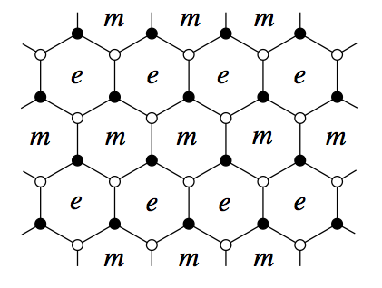
Figure 57: Magnetic ($m$) and electric ($e$) charges live on alternating rows of hexagons Kitaev (2006).

As the limit of extreme anisotropy is adiabatically connected, by continuously varying the couplings $J_{x,y,z}$, to all points of the “$A_{z}$ phase” of Kitaev’s model (we elaborate on the designation of the $A_{z}$ phase below), one may infer that the same identification of magnetic and electric charges holds for all other points in the $A_{z}$ phase. We now briefly define the $A_{z}$ phase, see Fig. 53.

Earlier, following Kitaev, we denoted the A phase as the one in which the couplings $J_{x},J_{y}$ and $J_{z}$ did not satisfy the triangle inequality (and for which the system was found to gapped even in the absence of a perturbation (Eqs. (229, 237)). This region can be further subdivided. The $A_{z}$ phase denotes that region of parameter space for which $|J_{z}|>|J_{x}|+|J_{y}|$ (i.e., the region of the $A$ phase in which the $J_{z}$ couplings are most dominant).

In a similar vein, replicating the above considerations to the cases in which $|J_{x}|\gg|J_{y,z}|$ (or $|J_{y}|\gg|J_{x,z}|$) we will find that in the $A_{x}$ ($A_{y}$) phase of Kitaev’s honeycomb model, vortices on alternating rows orthogonal to the $x$ (or $y$) direction will correspond to electric and magnetic charges. These charges obey the fusion rules of Eqs.(211, 212).

We now turn to explicit forms for the operators that translate vortices in Kitaev’s honeycomb model. These operators explicitly enable the braiding operations of excitations around each another. In Kitaev’s toric code model, there are two different types of vortex translation operators (related to the $X$ and $Z$ qubit operators). These are given by Eq. (278).

$${\cal{T}}_{cx}^{x}=\prod_{ij\in cx}\sigma^{x}_{ij},$$ (280)

With $cx$ a contour that bisects edges (ij).

When acting on the ground state, ${\cal{T}}_{cx}^{x}$ generates two plaquettes p with negative vorticity, $B_{p}=-1$. Similarly, when acting on a plaquette with a non-trivial vortex charge, ${\cal{T}}_{cx}^{x}$ shifts a vortex at plaquette $p_{1}$ to one at a plaquette $p_{2}$ if the plaquettes $p_{1}$ and $p_{2}$ lie at the endpoints of the contour $cx$ (have one side of the plaquette belonging to $cx$). When $cx$ forms a closed loop along one of the toric cycles, ${\cal{T}}_{cx}^{x}$ become one of the two symmetry operators $X_{1}$ or $X_{2}$.

Similarly, one may construct another type of vortex translation operator given by

$${\cal{T}}_{cz}^{z}=\prod_{ij\in cz}\sigma^{z}_{ij}.$$ (281)

In eq.(281), the edges (ij) lie on the contour $cz$. The operators ${\cal{T}}_{cz}^{z}$ shift or create vortices of the ”star” type: $A_{s}=-1$.

Analogous to the case of the operators ${\cal{T}}_{cx}^{x}$, the operators of eq.(281), become toric code symmetries when $cz$ forms a toric cycle. These are identified with $Z_{1,2}$.

Depending on the direction of the contour $\Gamma$ in eq.(243), it may become one of the two types of Eqs.(280,281).

For instance, if one considers a contour composed of xx and yy bonds on the hexagonal lattice then ${\cal{T}}_{\Gamma}$ is a product of $\sigma^{z}$ operators along the contour. When we shrink each zz bond to a single point in the strong coupling limit, the resulting zig-zag chain of ${\cal{T}}_{\Gamma}$ is of the same type as that of eq.(281).

Similarly, considering the same xx yy zig-zag contour c in the strong coupling limit of $|J_{x}|\gg|J_{y,z}|$, each xx type link reduces to a point and the geometry becomes akin to that of eq.(280).

X.6.5 Abelian Braiding statistics

We now explain the braiding rules of Kitaev’s toric code model and directly relate these to the operator representations of the translation operators of Eqs. (278) [or Eqs.(280,281)]. One may introduce an electric charge at site $s$: $A_{s}=-1$ and then apply the translation of Eq. (278) [or Eq. (281)] to translate along a contour $\Gamma$ the encircles a magnetic vortex (one with $B_{p}=-1$). In doing this operation, the translation operator becomes, similar to the Stokes’ type relation of Eq. (239), a phase factor of $(-1)$. To see this, we note that

$$\prod_{ij\in\Gamma}\sigma^{z}_{ij}=\prod_{p\in{\cal{A}}}B_{p},$$ (282)

where ${\cal{A}}$ is the region bounded by $\Gamma$. If there is a single magnetic vortex ($B_{p}=-1$) that is in ${\cal{A}}$ then Eq. (282) reduces to a factor of $(-1)$. We symbolically denote this result as in Fig. 58.

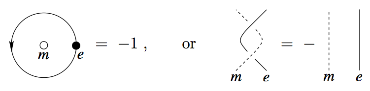
Figure 58: A pictorial view of the braiding rules between electric ($e$) and magnetic ($m$) charges Kitaev (2006).

Thus, one may regard the two quasi-particles of an “electric charge” ($A_{s}=-1$) and a “magnetic charge” as having a non-trivial statistics (leading to a factor of $(-1)$) when one particle is encircled around the other.

Along similar lines it is seen that taking an electric charge along a contour $\Gamma$ around another single electric charge (with no magnetic particles present) will lead to a trivial phase factor of $(+1)$. In this case, as no magnetic particles are present, $B_{p}=1$ everywhere within the contour $\Gamma$ and by Eq. (282), there is a trivial accumulated phase factor. Thus, the electric particles behave as bosons relative to themselves. The same similarly holds for magnetic particles amongst themselves. The fusion of an electric and magnetic particle- the dyon $\epsilon$ of Eq. (212)- is a fermionic particle Kitaev (2006). To see this, one may think about the motion of one dyon around the other. Naively, when considering the motion of one dyon (say, dyon number 1) around the other (dyon number 2) we might, at first, anticipate to have two factors of $(-1)$ as one the electric charge of dyon number 1 encircles the magnetic charge of dyon number 2 and similarly the electric charge of dyon number 1 revolves around the magnetic charge of dyon number 2. However, it should be kept in mind that dyon number 1 is rigid entity in which the magnetic charge in that dyon is held at a fixed relative position ${\bf r}$ relative to the electric charge of dyon number1. When the internal structure of the dyon is taken into account it is seen that while revolving dyon number 1 in a closed loop around dyon number 2, the world line of the magnetic particle in dyon number 1 winds around that of the electric particle of this dyon.

This additional internal winding leads to a third factor of $(-1)$ associated with the winding of dyon number 1 around dyon number 2. Thus, putting all of the pieces together, when one dyon is revolved around the other it accumulates a factor of $(-1)$. Thus, dyons do behave as fermions amongst themselves.

X.6.6 Relation between non-Abelian Ising Statistics & Toric Code Abelian Statistics

In subsections X.6.3,X.6.4, we discussed the explicit construction of defects in the Kitaev honeycomb model and their relation to those in the toric code model. Wootton et al. (2008) studied the general question as to how to construct non-Abelian anyons out of strings in the Abelian toric code model. Their elegant construct may be viewed as a discrete lattice variant of similar continuum constructions, e.g.,

X.6.7 Finite Temperature Behavior & Dynamics

As discussed in subsection X.6.2, the ground state (protected subspace of the code) is 4-fold degenerate (with Abelian ${\mathbb{Z}}_{2}\times{\mathbb{Z}}_{2}$ symmetry of Eqs. (276)). There is, furthermore, an energy gap to excitations.

Thermal effects in Kitaev’s toric code model (including those related to thermal fragility– the appearance of finite autocorrelation (or memory) times at all positive temperatures) and generalizations thereof were investigated by several groups Nussinov & Ortiz (2008a, b, 2009c, 2009a); Alicki et al. (2009); Iblisdir et al. (2009, 2010); Yoshida (2011). In simple physical terms, as a consequence of the $d=1$ symmetries that this system harbors and the generalized Elitzur theorem Batista & Nussinov (2005); Nussinov et al. (2012b) which we discussed, precisely as in the Ising chain, two defects can be created with a finite energy penalty and thereafter separated arbitrarily far apart from one another with no energy cost. Thus, as a consequence of this dimensional reduction, precisely as in the one-dimensional Ising mode, information initially stored in the qubits $Z_{i}$ (or $X_{i}$) will, at finite temperatures, be erased in a finite (i.e., system size independent) time scale. Beyond the specific information stored in these qubits, Kitaev’s toric code model genuinely has a 1D zero temperature Ising type transition and is disordered at any finite temperature Nussinov & Ortiz (2009c, a). That this is so is even more evident as the spectrum is that of two uncoupled circular Ising chains with each chain being of length $N_{S}$. [$2N_{s}$ is the total number of links of the original $D=2$ lattice.] This mapping has consequences for the system dynamics and thermodynamics. As Ising chains are disordered at any finite temperature, it is seen as stated above that, in thermal equilibrium state, this model is disordered at all non-zero temperatures ($\langle X_{\mu}\rangle=\langle Z_{\nu}\rangle=0$) and that there is a trivial critical point at temperature of

$$T_{c}^{Kitaev~{}Toric~{}Code}=0.$$ (283)

Due to the duality between Kitaev’s model and the Ising chains Nussinov & Ortiz (2009c, a), no non-trivial finite temperature spontaneous symmetry breaking or any other transition can take place. At any non-vanishing temperature, no matter how small, entropic contributions to the free energy overwhelm energy penalties and lead to a free energy which is everywhere analytic. Nevertheless, if temperatures far below the spectral gap may be achieved, the autocorrelation time $\tau$ associated with the topological invariants (the $d=1$ symmetries) of Eq. (276) can be made very large. That is, e.g., the autocorrelation function of the toric operators of Eq.(276),

$$\langle Z_{1}(0)Z_{1}(t)\rangle\sim\exp(-|t|/\tau),$$ (284)

with, at asymptotically low temperatures, $\tau=\exp(\beta\Delta)$ where $\Delta$ the spectral gap. Similar effects were found in some three dimensional variants of the Toric code model including those which further exhibit finite temperature transitions Nussinov & Ortiz (2008a, b). Several high dimensional systems reduce to Ising chains following a similar bond-algebraic mapping Nussinov et al. (2012b). Bounds of the form of Eq. (284) are not specific to the Kitaev model but are rather generic to any system with $d=1$ gauge like symmetries. The autocorrelation functions in these systems have a canonical one dimensional (chain type) character. In finite size systems, whenever the associated correlation length is larger than the system size, the system may appear ordered and a finite temperature crossover occurs when the correlation length is comparable to the system size Nussinov & Ortiz (2009c). The existence of these finite size effects is evidenced in the topological entanglement entropy Castelnovo & Chamon (2007). Quench dynamics of the entanglement entropy in Kitaev’s toric code model has been investigated Rahmani & Chamon (2010). Aspects of general topological quantum orders, associated symmetries, thermal effects (and their manifestations in correlations and stability of quantum information storage to perturbations) in Kitaev’s toric code and Kitaev’s honeycomb compass model and related models have been extensively discussed elsewhere, e.g., Dennis et al. (2002); Nussinov & Ortiz (2008a, b, 2009c, 2009a); Michnicki (2012); Bravyi & Terhal (2009); Cheng & Das Sarma (2012); Mazac & Hamma (2012); Son et al. (2012); Spyridon & Justyna (2011); Schuch et al. (2010); Kargarian (2009); Abasto & Zanardi (2009).

X.6.8 External fields, Disorder, Dilution, Coupling to Phonons & Photons

The effect of external fields was investigated in Trebst et al. (2011); Hamma & Lidar (2008); Tupitsyn et al. (2010); Vidal et al. (2009, 2009); Cobanera et al. (2010, 2011); Nussinov et al. (2012b) via numerous approaches (including, in certain cases, those of dualities and self-dualities). A very rich phase diagram harboring continuous and discontinuous transitions, multi-criticality, and dimensional reduction has been found. Recent works have also investigated the effects of disorder (realized as a distribution in the coupling constants) Wootton & Pachos (2011); Stark et al. (2011) and how such disorder may lead to localization of errors in a toric code quantum computing based schemes. The key steps in the solution of Kitaev’s honeycomb model that were outlined in section X.3 Chen & Nussinov (2008) do not change in such a case.

The relation between Kitaev’s honeycomb model and p-wave type BCS superconductors suggested in Chen & Nussinov (2008) that impurity bound states may appear. The effect of site dilution in Kitaev’s model was investigated in detail in Willans et al. (2010, 2011). Within the 90^∘ compass model wherein dilution trivially lowers the coordination number and removes bonds leading to higher degeneracy Nussinov & Ortiz (2008c). Similarly, dilution of the Kitaev model leads to extended zero energy states near each vacancy Willans et al. (2010, 2011). It is readily seen by, e.g., bond algebra considerations that were discussed earlier for the (undiluted) Kitaev model [as well as those employed for the diluted 90^∘ model Nussinov & Ortiz (2008c)], that Kitaev’s model will remain exactly solvable if the number of bonds is reduced due to dilution.

In the gapless phase, vacancies were shown to bind to plaquette fluxes. In the presence of an external magnetic field of strength $h$, interactions between induced moments lead to an attraction between the vacancies. In the absence of a vacancy in the bulk, the magnetic susceptibility $\chi\sim const$. A single vacancy leads to a susceptibility that scales as $\chi\sim|\ln h|$. For two nearby vacancies on the same sublattice, at low temperatures, $\chi\sim 1/(|h||\ln h|^{3/2})$ Willans et al. (2010, 2011). In the gapped phase, zero modes are localized by the vacancies.

Lastly, we briefly note the interesting work of Bonderson & Nayak (2012) where the stability of the Kitaev model and its degeneracy were illustrated for both (acoustic) phonon coupling as well as coupling with photons (via additional general Zeeman couplings in the low energy limit).

X.6.9 Doping with Kinetic Vacancies

Kitaev honeycomb models and Kitaev Heisenberg models doped with kinetic vacancies were explored in Mei (2011); You et al. (2011); Hyart et al. (2011). These systems describe doped systems with spin-1/2 fermions that hop on the lattice and that additionally exhibit a spin exchange terms similar to those of the Kitaev or Kitaev-Heisenberg models. Specifically, the spin Hamiltonians of the Kitaev and Kitaev-Heisenberg models of Eqs.(13, 113) respectively were, similar to $t-J$ models Fradkin (1991), augmented by a kinetic hopping term

$$H_{t}=-t\sum_{\langle ij\rangle\sigma}{\cal{P}}c_{i\sigma}^{\dagger}c_{j\sigma}{\cal{P}}.$$ (285)

A few standard words regarding the notation and $t-J$ type physics of Eq.(285) are due. The operator ${\cal{P}}$ in Eq. (285) projects out doubly occupied sites (lattice sites that harbor fermions of both spin $S=1/2$ up and down flavors). By virtue of this “no double occupancy” constraint, a fermion can only (with an amplitude $(-t)$) to an empty site (or, equivalently, a hole can kinetically hop to occupied neighboring sites). The spin exchange between sites that are occupied by fermions is given by the Kitaev or Kitaev-Heisenberg models of Eqs.(13,113). [In the standard $t-J$ models, the spin exchange between occupied sites is that of the rotationally invariant Heisenberg form (the scalar product between nearest neighbor spins).] In disparate analysis using the so-called “SU(2)” and “U(1) slave boson” methods respectively (in which the electronic creation operators $c_{i\sigma}^{\dagger}$ are decomposed into products of bosonic charge (holon) operators that carry SU(2) or U(1) degrees of freedom and fermionic “spinon” operators) , two works You et al. (2011); Hyart et al. (2011) suggested the emergence of spin triplet superconductivity with $p$ wave type pairing as the Kitaev type spin systems were doped when the Kitaev couplings were far stronger than the uniform spin exchange couplings in Eq. (113). Transitions separate the topologically trivial and non-trivial superconducting states at high and low dopings. At high ratios of the Heisenberg exchange couplings relative to the Kitaev couplings in Eq (113), the dominant Heisenberg exchange may, similar to the standard $t-J$ model, lead to spin singlet $d-$ wave type superconductivity. As highlighted by Hyart et al. (2011), the topological superconducting phase (in which pairs of counter-propagating Majorana modes appear) may appear over a much wider region of the phase diagram of the Kitaev-Heisenberg model than the Kitaev spin liquid phase itself in the absence of doping. If this model and its analysis indeed capture the quintessential features of doped Iridates, it might be easier to observe these non-trivial doped phase than the Kitaev type spin liquid of the Kitaev-Heisenberg model. The authors of You et al. (2011) suggest the appearance of a time reversal symmetry breaking sate (with $p_{x}+ip_{y}$ type pairing) while Hyart et al. (2011) arrive, within their calculations, at a lower energy time reversal invariant p-wave type pairing with Ising topological superconductivity. It remains to be seen which state is indeed favored by the complete energetic contributions. Another work Mei (2011) examined the Kitaev model at low dopings using a “dopon” representation that attempts to protects the $Z_{2}$ gauge structure of the Kitaev model and concluded that the doped Kitaev model is a Fermi liquid albeit with a temperature dependent Lorentz number (the ratio $L=\kappa/(\sigma T)$ where $\sigma$ is the thermal conductivity, $\sigma$ is the electric conductivity and $T$ is the temperature)) and a large Wilson ratio (the ratio between the zero-temperature magnetic susceptibility $\xi$ and the coefficient of the linear temperature term in the specific heat $\gamma$ ($C_{v}=\gamma T$) of a Fermi liquid, e. g., Varma et al. (2002)) .

X.6.10 Generalizations of Kitaev’s Models

Since Kitaev’s original works Kitaev (2006), many related models (in both two and three spatial dimensions) building on his original construct of his model have been advanced Chern (2010); Yao & Kivelson (2007); Nussinov & Ortiz (2009b); Yang et al. (2007); Si & Yu (2007, 2008); Yao et al. (2009); Wu et al. (2009); Ryu (2009); Mandal & Surendran (2009); Levin et al. (2011); Yao & Lee (2011); Nakai et al. (2011); Biswas et al. (2011); Lai & Motruich (2011b, c, a); Wang (2010); Tikhonov & Feigel man (2010); Tikhonov et al. (2011); Chua et al. (2011); Baskaran et al. (2009) most of which are exactly solvable. Many of these exactly solvable models flesh out rich phase diagrams and non-trivial excitations (and symmetries). One key principle in which the exact solvability of these models (and their equivalence (or duality) to far simple quadratic forms in various guises) becomes apparent is that of the bond algebras Nussinov & Ortiz (2009b); Cobanera et al. (2010, 2011); Nussinov & Ortiz (2008c) which were employed in the solution of Kitaev’s model presented in the preceding Section.

XI Conclusions

Complementing more standard theories with isotropic interactions between various fundamental fields (such as spin, charge, color, or more general “pseudo-spin”), there exists a plethora of physical systems in which the couplings between the pertinent internal degrees of freedom are direction dependent. The couplings in these “compass models” depend on the direction of the vectors connecting the interacting sites relative to a lattice (or continuum Cartesian or other directions). Such anisotropic direction dependent interactions are ubiquitous. Indeed, the anisotropic components of the interactions between dipoles when these are placed on lattices have precisely such a form. In compass models, external lattice (or other) directions lift the standard rotational invariance of the interactions. As we reviewed, in recent decades, numerous condensed matter systems have been discovered to host precisely such compass type interactions. The paradigmatic class of physical systems described by compass interactions is afforded by transition metal materials where the real space form of the pertinent electronic orbitals lead to exactly such direction dependent interactions. The associated orbital ordered have been observed to persist, in some materials, up to temperatures (that can range up to ${\cal{O}}(10^{3}$K)) that may significantly exceed magnetic ordering temperatures (when these are present) in these materials. Other primary examples of compass type interactions include diverse spin systems on frustrated lattices, bosonic and fermionic gases on optical lattices, materials with strong spin-orbit interactions, and other systems. Due to the anisotropic character of the interactions, the study of these systems is, by comparison to more standard rotationally invariant systems, a supremely interesting and challenging problem. Notably, as we reviewed for many particular compass Hamiltonians, some of these systems may be quantum liquids or, conversely, may lead low temperature phases of matter in which order is triggered by fluctuation effects. Rich phenomena, such as dimensional reduction and holography spawned by the unusual (exact or emergent) symmetries that these systems typically have, appear in these systems. The rich states of matter that compass models exhibit still remain largely unexplored. Items that have only started to being examined in recent years include the precise understanding of the nature of the phase transitions that they exhibit. To date, no effective field theories of these systems have been studied (nor even written down- our review includes one of the first general forms of these unusual anisotropic field theories). The intimate connections between compass models and topological quantum information (such as that exemplified by Kitaev’s model) and, in particular, topological states of matter (e.g., those displayed by recently discovered topological insulators) are likely to lead to new insights.

XII Acknowledgments

We have been very fortunate to closely interact with numerous colleagues on some of the systems described in this work. These include, amongst many others, C. Batista, M. Biskup, L. Chayes, H.-D. Chen, E. Cobaenra, M. Daghofer, T. P. Devereaux, E. Fradkin, P. Horsch, G. Khaliullin, D. Khomskii, S. Kumar, F. Nogueira, F. Mack, M. Mostovoy. A. Oles, K. Shtengel, K. Wohlfeld, J. Zaanen and P. Zoller. In particular, ZN is grateful to nearly a decade long interaction with G. Ortiz on many aspects of compass models. We are thankful for the understanding of these colleagues for not promptly writing other papers that need to be finished. We would like to thank our spouses for their patience and encouragement during this work. Work at Washington University (WU) in St Louis was partially supported by the National Science Foundation under NSF Grant number DMR- 1106293 (ZN) as well as the CMI of WU at the initial stages of this work. ZN is grateful to the hospitality of the IFW, Dresden during which central parts of this work were done.

XIII Appendix A: The bond algebra of the plaquette orbital model

In Eq. (46), following Wenzel & Janke (2009); Biskup & Kotecky (2010), we introduced the “plaquette orbital model”. We remarked therein that its local algebraic structure is similar to that of 90^∘ compass model on the square lattice [Eq. (1)]. In this very brief appendix, we clarify this observation and invoke the bond algebraic structure Cobanera et al. (2010, 2011); Ortiz et al. (2011); Nussinov et al. (2012b, a); Nussinov & Ortiz (2009b, 2008c) which we have earlier used in subsection X.3 in describing the exact solvability of Kitaev’s model on the honeycomb lattice

The Hamiltonian defining the plaquette orbital model is a sum of two types of terms (or “bonds”):
(A) $\tau^{x}_{i}\tau^{x}_{j}$ for all links that belong to the $A$ plaquette sublattice,$\langle ij\rangle\in A$.
(B) $\tau^{y}_{i}\tau^{y}_{j}$ for all links $\langle ij\rangle$ that belong to the $B$ plaquette sublattice.
The decomposition into the two plaquette ($A$ and $B$ sublattices) is shown in Fig. (8) Biskup & Kotecky (2010).

The algebra satisfied by these bonds is very simple and is encapsulated by the following relations

(i) The square of each bond is one.
(ii) Any two bonds that are of different type (i.e., one bond is of type A and the other is of type B) that share one common site anticommute: $\{\tau^{x}_{i}\tau^{x}_{j},\tau^{y}_{i}\tau^{y}_{k}\}=0$ with the curly brackets denoting the anticommutator. (By fiat, given the type of the interactions, $\langle ij\rangle\in A$ and $\langle ik\rangle\in B$.)
(iii) Bonds of different type commute if they share no common site: $[\tau^{x}_{i}\tau^{x}_{j},\tau^{y}_{k}\tau^{y}_{l}]=0$ (with $i,j,k,$ and $l$ corresponding to four different sites).
(iv) Any bond of type A commutes with any other bond of type A and, similarly, any bond of type B commutes with all bonds of the B type.

Thus, locally, each bond (having a square that is unity) anticommutes with two other neighboring bonds and commutes with the two other nearest neighbor bonds (as well all other bonds on the lattice).

The bond algebra associated with the 90^∘ compass model of Eq. (1) is very much like that of the plaquette orbital model. This system has a decomposition into two types of similar bonds:

(a) $\tau^{x}_{i}\tau^{x}_{j}$ on all horizontal links.
(b) $\tau^{y}_{i}\tau^{y}_{j}$ on all vertical links.

The algebra satisfied by these bonds is specified by a similar list:

(i) The square of each bond is one.
(ii) Any two bonds that are of different type that share one common site anticommute: $\{\tau^{x}_{i}\tau^{x}_{j},\tau^{y}_{i}\tau^{y}_{k}\}=0$. newline (iii) Bonds of different type commute if they share no common site: $[\tau^{x}_{i}\tau^{x}_{j},\tau^{y}_{k}\tau^{y}_{l}]=0$ (with $i,j,k,$ and $l$ corresponding to four different sites).
(iv) Any horizontal bond commutes with any other horizontal bond and, analogously, any vertical bond commutes with all vertical bonds.

The local algebra is congruent to that of the plaquette orbital model: each bond anticommutes with two out of its four nearest neighbors. This equal structure implies that in their Cayley tree (or Bethe lattice) approximations, the 90^∘ and the plaquette compass model are identical.

XIV Appendix B: Gell-Mann Matrices

The Gell-Mann matrices are a representation of the infinitesimal generators of the special unitary group SU(3). This group has dimension eight and therefore it has a set with eight linearly independent generators, which can be written as $\lambda_{i}$, with $i$ taking values from 1 to 8. They obey the commutation relations

$$[\lambda_{i},\lambda_{j}]=\frac{i}{2}f^{ijk}\lambda_{k},$$ (286)

where a sum over the index $k$ is implied. The constants $f^{ijk}$ are $f^{123}=1$, $f^{147}=f^{165}=f^{246}=f^{257}=f^{345}=f^{376}=1/2$ and $f^{458}=f^{678}=\sqrt{3}/2$ and are antisymmetric in the three indices. The Gell-Mann matrices representations involving $3\times 3$ matrices, that act on complex vectors with 3 entries. They have the additional properties that are traceless, Hermitian, and obey the relation Tr$(\lambda_{i}\lambda_{j})$ $=2\delta_{ij}$.

$$\lambda_{1}=\begin{pmatrix}0&1&0\\ 1&0&0\\ 0&0&0\\ \end{pmatrix},\quad\lambda_{2}=\begin{pmatrix}0&-i&0\\ i&0&0\\ 0&0&0\\ \end{pmatrix},\quad\lambda_{3}=\begin{pmatrix}1&0&0\\ 0&-1&0\\ 0&0&0\\ \end{pmatrix}$$

$$\lambda_{4}=\begin{pmatrix}0&0&1\\ 0&0&0\\ 1&0&0\\ \end{pmatrix},\quad\lambda_{5}=\begin{pmatrix}0&0&-i\\ 0&0&0\\ i&0&0\\ \end{pmatrix},\quad\lambda_{6}=\begin{pmatrix}0&0&0\\ 0&0&1\\ 0&1&0\\ \end{pmatrix}$$

$$\lambda_{7}=\begin{pmatrix}0&0&0\\ 0&0&-i\\ 0&i&0\\ \end{pmatrix},\quad\lambda_{8}=\frac{1}{\sqrt{3}}\begin{pmatrix}1&0&0\\ 0&1&0\\ 0&0&-2\\ \end{pmatrix}$$

The matrices $\lambda_{3}$ and $\lambda_{8}$ commute. Three independent SU(2) subgroups are formed by the elements of vectors ${\bm{\mu}}^{1}$, ${\bm{\mu}}^{2}$ and ${\bm{\mu}}^{3}$, where ${\bm{\mu}}^{1}=\frac{1}{2}(\lambda_{1},\lambda_{2},\lambda_{3})$, ${\bm{\mu}}^{2}=\frac{1}{2}(\lambda_{4},\lambda_{5},\lambda_{+})$, and ${\bm{\mu}}^{3}=\frac{1}{2}(\lambda_{6},\lambda_{7},\lambda_{-})$. Here the $\lambda_{+}$, $\lambda_{-}$ are linear combinations of $\lambda_{3}$ and $\lambda_{8}$: $\lambda_{\pm}=\lambda_{3}\cos\left(\frac{2\pi}{3}\right)\pm\lambda_{8}\sin\left(\frac{2\pi}{3}\right)$, so that, as is expected for a SU(2) spin $1/2$, the commutator $[{\bm{\mu}}_{1}^{\gamma},{\bm{\mu}}_{2}^{\gamma}]=\frac{i}{2}{\bm{\mu}}_{3}^{\gamma}$, for each $\gamma=1,2,3$.

The operators

$$\hat{R}^{+}=\begin{pmatrix}0&0&1\\ 1&0&0\\ 0&1&0\end{pmatrix};\hat{R}^{-}=\begin{pmatrix}0&1&0\\ 0&0&1\\ 1&0&0\end{pmatrix}$$ (287)

rotate the vectors $\bm{\mu}$ onto eachother: ${\bm{\mu}^{2}}=\hat{R}^{-}{\bm{\mu}^{1}}\hat{R}^{+}$

XV Appendix C: Classical & Quantum fluctuations in the large $n$ limit

The large $n$ limit (see section III.2) of the theory of Eq. (150) is exactly solvable. As such, it allows us to easily point out to a difference between the classical and quantum theories. In the large $n$ limit of the classical system, order appears in $D$ dimensional system appears if and only if the classical (lowest order (${\cal{O}}(1/n)^{0}$)) self-energy diagram stemming from the Boltzmann distribution of harmonic modes (and its related equipartition theorem)

$$\Sigma^{(0)}_{cl}=\sum_{\alpha}\int\frac{d^{D}k}{(2\pi)^{D}}\frac{1}{v_{\alpha}({\bf k})+\mu}$$ (288)

does not diverge as the “mass” $\mu$ veers towards $[-\min_{k,\alpha}\{v_{\alpha}({\bf k})]$. The integration in Eq. (288) is performed over the first Brillouin zone- a region of finite volume. Thus, $\Sigma^{(0)}_{cl}$ can diverge only from infra-red contributions. In systems in which the mode spectra $v_{\alpha}({\bf k})$ disperse quadratically about their minimum, the relevant integral converges in dimensions $D>2$ but fails to converge in low dimensions due to the large relative phase space volume of low energy modes. Quantum mechanically, in large $n$ systems, see, e.g., Nussinov (2004); Serral Gracia & Nieuwenhuizen (2004), the corresponding self-energy is governed by the Bose function set by the modes $\omega_{k}$. The pertinent zero temperature dispersion of $v_{\alpha}({\bf k})$ in the argument of the integrand governing the convergence or divergence of 288 in the classical case is replaced in quantum case by the square root forms $\sqrt{v_{\alpha}({\bf k})}$. Qualitatively similar Bose type distributions and dispersions are found in 1/S calculations. As power counting suggests, the convergence of the integral and thus the character of the fluctuations arising from classical and quantum effects are different. It is possible to have ordering of the quantum system at zero temperature while the classical counterpart of Eq. (288) exhibits an infra-red divergence. Such a case arises in two-dimensional ferromagnets Precisely this sort of situation arises in the 120^∘ compass model- the large $n$ quantum version of the model exhibits low temperature order (quantum order out of disorder) yet its classical counterpart exhibits no finite temperature order. As it will turn out, however, once the 120^∘ system is constrained to its original $n=2$ component version, both classical thermal fluctuations and quantum effects lead to similar sorts of ordering.

References

- Abasto & Zanardi (2009) Abasto, D. F. & Zanardi, P. (2009). Thermal states of the Kitaev honeycomb model: a bures metric analysis. Physical Review A 79, 012321.
- Abragam & Bleaney (1970) Abragam, A. & Bleaney, B. (1970). Electron Paramagnetic Resonance of Transition Ions. Clarendon Press.
- Aharonov & Bohm (1959) Aharonov, Y. & Bohm, D. (1959). Significance of electromagnetic potentials in quantum theory. Physical Review 115, 485.
- Ahlbrecht et al. (2009) Ahlbrecht, A., Georgiev, L. S. & Werner, R. F. (2009). Implementation of clifford gates in the ising-anyon topological quantum computer. Physical Review A 79, 032311.
- Alicea (2010) Alicea, J. (2010). Majorana fermions in a tunable semiconductor device. Phys. Rev. B 81, 125318.
- Alicea et al. (2011) Alicea, J., Oreg, Y., Refael, G., von Oppen, F. & Fisher, M. P. A. (2011). Non-abelian statistics and topological quantum information processing in 1d wire networks. Nature Physics 7, 412.
- Alicki et al. (2009) Alicki, R., Fannes, M. & Horodecki, M. (2009). On thermalization in Kitaev’s 2D model. J. of Phys. A 42, 065303.
- Anderlini et al. (2007) Anderlini, M., Lee, P. J., Brown, B. L., Sebby-Strabley, J., Phillips, W. D. & Porto, J. V. (2007). Controlled exchange interaction between pairs of neutral atoms in an optical lattice. Nature 448, 452.
- Anderson (1951) Anderson, P. W. (1951). Limits on the energy of the antiferromagnetic ground state. Phys. Rev. 83, 1260.
- Anderson (1959) Anderson, P. W. (1959). New approach to the theory of superexchange interactions. Phys. Rev. 115, 2.
- Avron et al. (2003) Avron, J. E., Osadchy, D. & Seiler, R. (2003). A topological look at the quantum Hall effect. Physics Today , 38.
- Balents (2011) Balents, L. (2011). Weyl electrons kiss. Physics 4, 36.
- Ballhausen (1962) Ballhausen, C. (1962). Introduction to Ligand Field Theory. McGraw Hill.
- Baraban et al. (2009) Baraban, M., Zikos, M., Bonesteel, N. & Simon, S. H. (2009). Numerical analysis of quasiholes of the moore-read wavefunction. Phys. Rev. Lett. 103, 076801.
- Barkeshli & McGreevy (2012) Barkeshli, M. & McGreevy, J. (2012). Continuous transitions between composite fermi liquid and landau fermi liquid: a route to fractionalized mott insulators. arXiv:1206.6530 .
- Baskaran et al. (2007) Baskaran, G., Mandal, S. & Shankar, R. (2007). Exact results for spin dynamics and fractionization in the Kitaev model. Phys. Rev. Lett. 98, 247201.
- Baskaran et al. (2009) Baskaran, G., Santhosh, G. & Shankar, R. (2009). Exact quantum spin liquids with fermi surfaces in spin-half models. arXiv:0908.1614 .
- Baskaran et al. (2008) Baskaran, G., Sen, D. & Shankar, R. (2008). Spin-S Kitaev model: Classical ground states, order from disorder, and exact correlation functions. Phys. Rev. B 78, 115116.
- Batista & Trugman (2004) Batista, C. & Trugman, S. (2004). Exact ground states of a frustrated 2d magnet: Deconfined fractional excitations at a first-order quantum phase transition. Phys. Rev. Lett. 93, 217202.
- Batista & Nussinov (2005) Batista, C. D. & Nussinov, Z. (2005). Generalized elitzur’s theorem and dimensional reductions. Phys. Rev. B 72, 045137.
- Beenakker (2011) Beenakker, C. W. J. (2011). Search for majorana fermions in superconductors. arXiv:1112.1950 .
- Beigi et al. (2011) Beigi, S., Shor, P. W. & Whalen, D. (2011). The quantum double model with boundary: Condensations and symmetries. Communications in Mathematical Physics 306, 663.
- Berlin & Kac (1952) Berlin, T. H. & Kac, M. (1952). The spherical model of a ferromagnet. Phys. Rev. 86, 821.
- Bernevig et al. (2006) Bernevig, B. A., Hughes, T. L. & Zhang, S. C. (2006). Quantum spin Hall effect and topological phase transition in hgte quantum wells. Science 314, 1757.
- Bernevig & Zhang (2006) Bernevig, B. A. & Zhang, S. C. (2006). Quantum spin Hall effect. Phys. Rev. Lett. 96, 106802.
- Berry (1984) Berry, M. V. (1984). Quantal phase factors accompanying adiabatic changes. Proceedings of the Royal Society London, Series A 392, 45.