Chord distribution along a line in the local Universe

Este documento describe ..

Abstract

A method is developed to compute the chord length distribution along a line which intersects a cellular Universe. The cellular Universe is here modeled by the Poissonian Voronoi Tessellation (PVT) and by a non-Poissonian Voronoi Tessellation (NPVT). The distribution of the spheres is obtained from common approximations used in modeling the volumes of Voronoi Diagrams.

We give analytical formulas for the distributions of the lengths of chords in both the PVT and NPVT. The astrophysical applications are made to the real Eso Slice Project and to an artificial slice of galaxies which simulates the 2dF Galaxy Redshift Survey.

statistical distributions galaxies clusters of galaxies

0.1 Introduction

The study of the spatial periodicity in the spatial distribution of quasars started with Tifft (1973, 1980, 1995). A recent analysis of Bell & McDiarmid (2006), in which 46 400 quasars were processed, quotes a periodicity near $\Delta z$ =0.7. The study of periodicity in the spatial distribution of galaxies started with Broadhurst et al. (1990), where the data from four distinct surveys at the north and south Galactic poles were processed. He found an apparent regularity in the galaxy distribution with a characteristic scale of 128 Mpc. Recently, Hartnett (2009b, a) quotes peaks in the distribution of galaxies with a periodicity near $\Delta z$ =0.01. More precisely, he found a regular real space radial distance spacings of 31.7 Mpc, 73.4 Mpc, and 127 Mpc. On adopting a theoretical point of view, the periodicity is not easy to explain. A framework which explains the periodicity is given by the cellular universe in which the galaxies are situated on the faces of irregular polyhedrons. A reasonable model for the cellular universe is the Poissonian Voronoi Tessellation (PVT); another is the non-Poissonian Tessellation (NPVT). Some properties of the PVT can be deduced by introducing the averaged radius of a polyhedron, $\bar{R}$. The astronomical counterpart is the averaged radius of the cosmic voids as given by the Sloan Digital Sky Survey (SDSS) R7, which is $\bar{R}=\frac{18.23}{h}Mpc$, see Pan et al. (2012). The number of intercepted voids, $n_{v}$, along a line will be $n_{v}=\frac{L}{\bar{l}}$, where $L$ is the considered length and $\bar{l}$ the average chord. On assuming $\bar{l}=\frac{4}{3}\bar{R}$, $n_{V}=\frac{3L}{4\bar{R}}$. The astronomical counterpart of the line is the pencil beam catalog, a cone characterized by a narrow solid angle, see Szalay et al. (1993). The number of galaxies intercepted on the faces of the PVT will follow the photometric rules as presented in Zaninetti (2010), and Figure 1 reports the theoretical number of galaxies for a pencil beam characterized by the solid angle $\Omega$ of 60 deg².

Figure 1: The number of galaxies as a function of the distance for a pencil beam catalog of $\Omega=60$ deg². The curve was calibrated on the data of the 2dF Galaxy Redshift Survey (2dFGRS) which has $\Omega=1500$ deg². Adapted from Figure 4 in Zaninetti (2010).

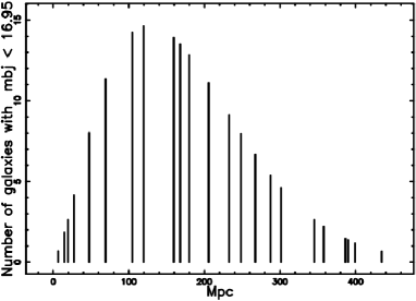
According to the cellular structure of the local universe, the number of galaxies as a function of distance will follow a discontinuous rather than a continuous increase or decrease.

We can therefore raise the following questions.

• Can we find an analytical expression for the chord length distribution for lines which intersect many PVT or NPVT polyhedrons?

• Can we compare the observed periodicity with the theoretical ones?

In order to answer these questions, Section 0.2 briefly reviews the existing knowledge of the chord’s length in the presence of a given distribution of spheres. Section 0.3 derives two new equations for the chord’s distribution in a PVT or NPVT environment. Section 0.4 is devoted to a test of the new formulas against a real astronomical slice and against a simulated slice.

0.2 The basic equations

This Section reviews a first example of deducing the average chord of spheres having the same diameter and the general formula for the chord’s length when a given distribution for the spheres’ diameters is given.

0.2.1 The simplest example

We calculate the average length of all chords of spheres having the same radius $R$. Figure 2 reports a section of a sphere having radius $R$ and chord length $l$.

Figure 2: The section of an intersected sphere of unit radius. The chord is drawn with the thicker line and marked with $l$.

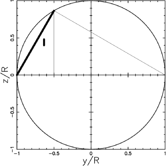
The Pythagorean theorem gives

$$l=\sqrt{2(1+y)}R\quad,$$ (1)

and the average chord length is

$$<l>=\frac{1}{2}\int_{-1}^{+1}\sqrt{2(1+y)}Rdy=\frac{4}{3}R\quad.$$ (2)

0.2.2 The probabilistic approach

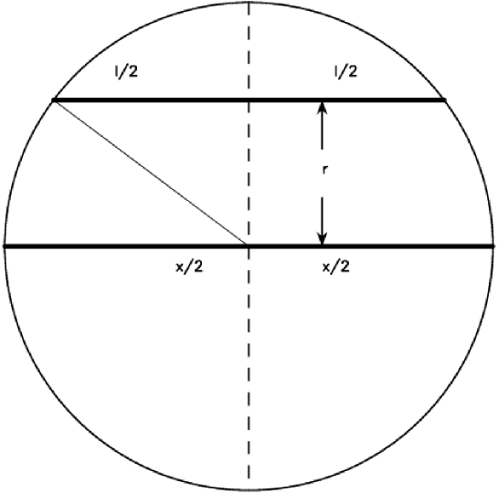
The starting point is a probability density function (PDF) for the diameter of the voids, $F(x)$, where $x$ indicates the diameter. The probability, $G(x)dx$, that a sphere having diameter between $x$ and $x+dx$ intersects a random line is proportional to their cross section

$$G(x)dx=\frac{\frac{\pi}{4}x^{2}F(x)dx}{\int_{0}^{\infty}\frac{\pi}{4}x^{2}F(x)dx}=\frac{x^{2}F(x)dx}{<x^{2}>}\quad.$$ (3)

Given a line which intersects a sphere of diameter $x$, the probability that the distance from the center lies in the range $r,r+dr$ is

$$p(r)=\frac{2\pi rdr}{\frac{\pi}{4}x^{2}}\quad,$$ (4)

and the chord length is

$$l=\sqrt{x^{2}-4r^{2}}\quad,$$ (5)

see Figure 3.

Figure 3: The section having diameter $x$ of the intersected sphere. The chord is drawn with the thicker line and marked with $l$; the distance between chord and center is $r$.

The probability that spheres in the range $(x,x+dx)$ are intersected to produce chords with lengths in the range $(l,l+dl)$ is

$$G(x)\,dx\frac{2l\,dl}{x^{2}}=\frac{2l\,dl}{<x^{2}>}F(x)dx\quad.$$ (6)

The probability of having a chord with length between $(l,l+dl)$ is

$$g(l)=\frac{2l}{<x^{2}>}\int_{l}^{\infty}F(x)dx\quad.$$ (7)

This integral will be called fundamental and the previous demonstration has been adapted from Ruan et al. (1988). A first test of the previous integral can be done inserting as a distribution for the diameters a Dirac delta function

$$F(x)=\delta(x-2\,R)\quad.$$ (8)

As a consequence, the following PDF for chords is obtained:

$$g(l)=\frac{1}{2}\frac{l}{R^{2}}\quad,$$ (9)

which has an average value

$$<l>=\frac{4}{3}R\quad.$$ (10)

We have therefore obtained, in the framework of the probabilistic approach, the same result deduced with elementary methods, see Equation (2).

0.3 Voronoi diagrams

This section reviews the distribution of spheres which approximates the volume distribution for PVT and NPVT, explains how to generate NPVT seeds, and derives two new formulas for the distributions of the chords.

0.3.1 PVT volume distribution

We analyze the gamma variate $H(x;c)$ (Kiang (1966))

$$H(x;c)=\frac{c}{\Gamma(c)}(cx)^{c-1}\exp(-cx),$$ (11)

where $0\leq x<\infty$, $c\leavevmode\nobreak\ >0$, and $\Gamma$ is the gamma function. The Kiang PDF has a mean of

$$\mu=1,$$ (12)

and variance

$$\sigma^{2}=\frac{1}{c}.$$ (13)

A new PDF due to Ferenc & Néda (2007) models the normalized area/volume in 2D/3D PVT

$$FN(x;d)=C\times x^{\frac{3d-1}{2}}\exp{(-(3d+1)x/2)},$$ (14)

where $C$ is a constant,

$$C=\frac{\sqrt{2}\sqrt{3\,d+1}}{2\,{2}^{3/2\,d}\left(3\,d+1\right)^{-3/2\,d}\Gamma\left(3/2\,d+1/2\right)},$$ (15)

and $d(d=1,2,3)$ is the dimension of the space under consideration. We will call this function the Ferenc–Neda PDF; it has a mean of

$$\mu=1,$$ (16)

and variance

$$\sigma^{2}=\frac{2}{3d+1}.$$ (17)

The Ferenc–Neda PDF can be obtained from the Kiang function (Kiang (1966)) by the transformation

$$c=\frac{3d+1}{2},$$ (18)

and as an example $d=3$ means $c=5$.

0.3.2 NPVT volume distribution

The most used seeds which produce the tessellation are the so called Poissonian seeds. In this, the most explored case, the volumes are modeled in 3D by a Kiang function, Equation (11), with $c=5$. An increase of the value of $c$ of the Kiang function produces more ordered structures and a decrease, less ordered structures. A careful analysis of the distribution in effective radius of the Sloan Digital Sky Survey (SDSS) DR7 indicates $c\approx 2$, see Zaninetti (2012). Therefore the normalized distribution in volumes which models the voids between galaxies is

$$H(x;2)=4\,x{{\rm e}^{-2\,x}}\quad.$$ (19)

0.3.3 NPVT seeds

The 3D set of seeds which generate a distribution in volumes with $c\approx 2$ for the Kiang function (19) is produced with the following algorithm. A given number, $N_{H}$, of forbidden spheres having radius $R_{H}$ are generated in a 3D box having side $L$. Random seeds are produced on the three spatial coordinates; those that fall inside the forbidden spheres are rejected. The volume forbidden to the seeds occupies the following fraction, $f$, of the total available volume

$$f=\frac{N_{H}\frac{4}{3}\pi R_{H}^{3}}{L^{3}}\quad.$$ (20)

The value of $c\approx 2$ for the Kiang function is found by increasing progressively $N_{H}$ and $R_{H}$.

0.3.4 PVT chords

The distribution in volumes of the 3D PVT can be modeled by the modern Ferenc–Neda PDF (14) by inserting $d=3$. The corresponding distribution in diameters can be found using the following substitution

$$x=\frac{4}{3}\pi(\frac{y}{2})^{3}\quad,$$ (21)

where $y$ represents the diameter of the volumes modeled by the spheres. Therefore the PVT distribution in diameters is

$$F(y)={\frac{3125}{62208}}\,{\pi}^{5}{{\it y}}^{14}{{\rm e}^{-5/6\,\pi\,{{\it y}}^{3}}}\quad.$$ (22)

Figure  4 displays the PDF of the diameters already obtained.

Figure 4: PDF $F(y)$ for the PVT diameters.

We are now ready to insert in the fundamental Equation (7) for the chord length a PDF for the diameters. The resulting integral is

$$g(l)={\frac{243}{1540}}\,{\frac{l{5}^{2/3}\sqrt[3]{6}{\pi}^{2/3}}{\Gamma\left(2/3\right)\left({{\rm e}^{\pi\,{l}^{3}}}\right)^{5/6}}}+{\frac{81}{616}}\,{\frac{{l}^{4}{5}^{2/3}\sqrt[3]{6}{\pi}^{5/3}}{\Gamma\left(2/3\right)\left({{\rm e}^{\pi\,{l}^{3}}}\right)^{5/6}}}$$

$$+{\frac{135}{2464}}\,{\frac{{l}^{7}{5}^{2/3}\sqrt[3]{6}{\pi}^{8/3}}{\Gamma\left(2/3\right)\left({{\rm e}^{\pi\,{l}^{3}}}\right)^{5/6}}}+{\frac{75}{4928}}\,{\frac{{l}^{10}{5}^{2/3}\sqrt[3]{6}{\pi}^{11/3}}{\Gamma\left(2/3\right)\left({{\rm e}^{\pi\,{l}^{3}}}\right)^{5/6}}}$$

$$+{\frac{125}{39424}}\,{\frac{{l}^{13}{5}^{2/3}\sqrt[3]{6}{\pi}^{14/3}}{\Gamma\left(2/3\right)\left({{\rm e}^{\pi\,{l}^{3}}}\right)^{5/6}}}$$ (23)

This first result should be corrected due to the fact that the PDF of the diameters, see Figure 4, is $\approx$ 0 up to a diameter of $\approx$ 0.563. We therefore introduce the following translation

$$U=L+a\quad,$$ (24)

where $L$ is the random chord and $a$ the amount of the translation. The new translated PDF, $g_{1}(u;a)$, takes values $u$ in the interval $[-a,(6-a)]$. Due to the fact that only positive chords are defined in the interval $[0,(6-a)]$, a new constant of normalization should be introduced

$$g_{2}(u;a)=Cg_{1}(u;a),\quad where$$ (25)

$$C=\frac{1}{\int_{0}^{6-a}g_{1}(u;a)du}\quad.$$ (26)

The last transformation of scale is

$$R=\frac{U}{b}\quad,$$ (27)

and the definitive PDF for chords is

$$g_{3}(r;a,b)=\frac{g_{2}(\frac{u}{b};a)}{b}\quad.$$ (28)

The resulting distribution function will be

$$DF_{1,3}(r:a,b)=\int_{0}^{r}g_{3}(r;a,b)dr\quad.$$ (29)

We are now ready for a comparison with the distribution function ,$F_{L_{1,3}}$, for chord length , $L_{1,3}$ in $V_{p}(1,3)$, see formula (5.7.6) and Table 5.7.4 in Okabe et al. (2000). Table 1 shows the average diameter, variance, skewness, and kurtosis of the already derived $g_{3}(r;a,b)$. The parameter $b$ should match the average value of the PDF in Table 5.7.4 of Okabe et al. (2000).

Table 1: The parameters of $g_{3}(r;a,b)$, Eq. (28), relative to the PVT case when $b=1.624$ and $a=0.563$.

$$\begin{array}[]{ll}\hline\cr Parameter&value\\ \vskip 3.0pt plus 1.0pt minus 1.0pt\cr\hline\cr\vskip 3.0pt plus 1.0pt minus 1.0pt\cr Mean&0.662\\ \vskip 3.0pt plus 1.0pt minus 1.0pt\cr\hline\cr Variance&0.144\\ \vskip 3.0pt plus 1.0pt minus 1.0pt\cr\hline\cr Skewness&0.274\\ \hline\cr Kurtosis&-0.581\\ \hline\cr\end{array}$$

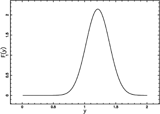
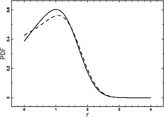
The behavior of $g_{3}(r;a,b)$ is shown in Figure 5.

Figure 5: PDF $g_{3}(r;a,b)$ (full line) for chord length as a function of $r$ when $b=2.452$, $a=0.563$, which means $<r>=1$, and the mathematical PDF (dashed line) as extracted from Table 5.7.4 in Okabe et al. (2000), PVT case.

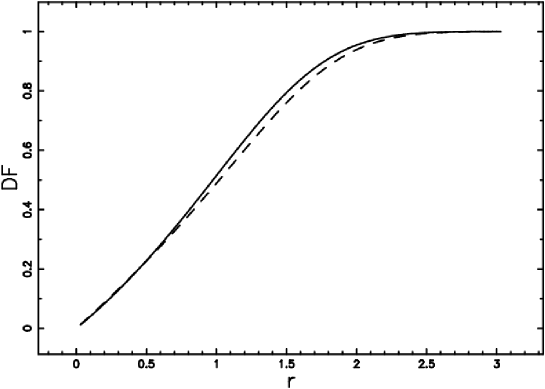
The behavior of $DF_{1,3}(r:a,b)$ is shown in Figure 6.

Figure 6: Distribution function $DF_{1,3}(r:a,b)$ (full line) for chord length as a function of $r$ when $b=2.452$, $a=0.563$, which means $<r>=1$, and the mathematical DF (dashed line) as extracted from Table 5.7.4 in Okabe et al. (2000), PVT case.

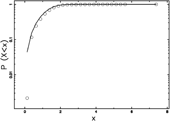
Consider a 3D PVT and suppose it intersects a randomly oriented line $\gamma$: the theoretical distribution function $DF_{1,3}(r:a,b)$ as given by Eq. (29) and the results of a numerical simulation can be compared. We start from $900000$ 3D PVT cells and we process $9947$ chords which were obtained by adding together the results of $40$ triples of mutually perpendicular lines. The numerical distribution of Voronoi lines is shown in Figure 7 with the display of $DF_{1,3}(r:a,b)$.

Figure 7: Comparison between data (empty circles) and theoretical curve , $DF_{1,3}(r:a,b)$, (continuous line) of the chord length distribution when $b=2.452$, $a=0.563$, which means $<r>$ =1; PVT case. The maximum distance between the two curves is $d_{max}=0.01$.

0.3.5 NPVT chords

In the case here analyzed, see the PDF in volumes as given by Equation(19), the NPVT distribution in diameters which corresponds to $c=2$ in volumes is

$$F(y)=1/3\,{\pi}^{2}{{\it y}}^{5}{{\rm e}^{-1/3\,\pi\,{{\it y}}^{3}}}\quad,$$ (30)

where $y$ represents the diameter of the volumes modeled by spheres. We now insert in the fundamental Equation (7) for the chord length a PDF for the diameters as given by the previous equation. The resulting integral, which models the NPVT chords, is

$$g_{NPVT}(l)=\frac{l{\pi}^{8/3}\sqrt[3]{3}\left(3+\pi\,{l}^{3}\right)}{5\,\Gamma\left(2/3\right){\pi}^{2}\sqrt[3]{{{\rm e}^{\pi\,{l}^{3}}}}}\quad.$$ (31)

We now make the following translation

$$U=L+a\quad.$$ (32)

The new translated PDF is $g_{NPVT,1}(u;a)$ and the new constant of normalization is

$$g_{NPVT,2}(u;a)=C_{NPVT}g_{NPVT,1}(u;a),\quad where$$ (33)

$$C_{NPVT}=\frac{1}{\int_{0}^{6-a}g_{NPVT,1}(u;a)du}$$ (34)

The transformation of scale is

$$R=\frac{U}{b}\quad,$$ (35)

and the definitive PDF for NPVT chords is

$$g_{NPVT,3}(r;a,b)=\frac{g_{NPVT,2}(\frac{u}{b};a)}{b}\quad.$$ (36)

The behavior of the NPVT $g_{NPVT,3}(r;a,b)$ is shown in Figure 8.

Figure 8: PVT PDF $g_{3}(r;a,b)$ for chord length as a function of $r$, when $b=2.452$, $a=0.563$ (full line), and NPVT PDF $g_{NPVT,3}(r;a,b)$ when $b=1.741$, $a=0.36$ (dashed line). In both cases $<r>$=1.

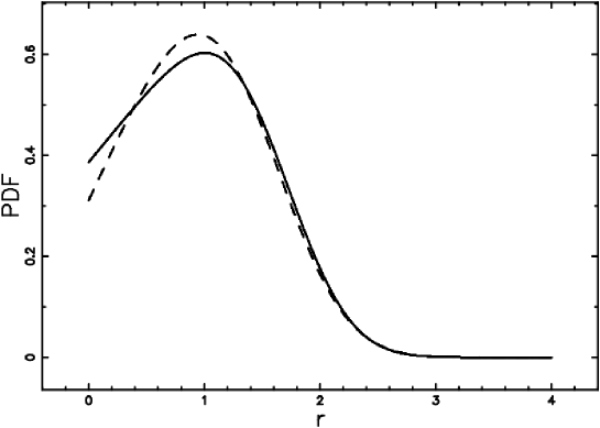
Table 2 shows the average diameter, variance, skewness, and kurtosis of the already derived NPVT $g_{NPVT,3}(r;a,b)$.

Table 2: The parameters of $g_{npvt,3}(r;a,b)$, Eq. (31), relative to the NPVT case when $b=1.153,a=0.36$.

$$\begin{array}[]{ll}\hline\cr Parameter&value\\ \vskip 3.0pt plus 1.0pt minus 1.0pt\cr\hline\cr\vskip 3.0pt plus 1.0pt minus 1.0pt\cr Mean&0.662\\ \vskip 3.0pt plus 1.0pt minus 1.0pt\cr\hline\cr Variance&1.153\\ \vskip 3.0pt plus 1.0pt minus 1.0pt\cr\hline\cr Skewness&0.324\\ \hline\cr Kurtosis&-0.442\\ \hline\cr\end{array}$$

The resulting distribution function with scale will be

$$DF_{NPVT}(r:a,b)=\int_{0}^{r}g_{NPVT,3}(r;a,b)dr\quad.$$ (37)

Also in this case we produce $900000$ 3D NPVT cells and we process $9947$ chords which were obtained by adding together the results of $40$ triples of mutually perpendicular lines. The numerical distribution of Voronoi lines is shown in Figure 9 with the display of $DF_{NPVT}(r:a,b)$.

Figure 9: Comparison between data (empty circles) and theoretical curve (continuous line) of the chord length distribution when $b=1.741$, $a=0.36$, which means $<r>$ =1; NPVT case. The maximum distance between the two curves is $d_{max}=0.03$. The fraction of volume forbidden to the NPVT seeds is $f=16\%$.

0.4 Astrophysical applications

At the moment of writing, it is not easy to check the already found PDFs for the chord distribution in the local Universe. This is because research has been focused on the intersection of the maximal sphere of voids between galaxies with the mid-plane of a slab of galaxies, as an example see Figure 1 in Pan et al. (2012). Conversely, the organization of the observed patterns in slices of galaxies in irregular pentagons or hexagons having the property of a tessellation has not yet been developed. We briefly recall that in order to compute the length in a given direction of a slice of galaxies the boundary between a region and another region should be clearly computed in a digital way. In order to find the value of scaling, $b$, which models the astrophysical chords, some first approximate methods will be suggested. A first method starts from the average chord for monodispersed bubble size distribution (BSD) which are bubbles of constant radius $R$, see (2), and approximates it with

$$<l>=\frac{4}{3}<R>\quad,$$ (38)

where $R$ has been replaced by $<R>$. We continue by inserting $<R>=18.23h^{-1}$ Mpc, which is the effective radius in SDSS DR7, see Table 6 in in Zaninetti (2012), and in this case $b=42.32h^{-1}$ Mpc. A comparison should be made with the scaling of the probability of obtaining a cross-section of radius $r$, which is $\frac{31.33}{h}$ Mpc, see Zaninetti (2012). The PDF of the chord conversely has average value given by the previous equation (38) and therefore $b$ is 4/3 bigger.

We now report a pattern of NPVT series of chords superposed on a astronomical slice and a simulation of an astronomical slice in the PVT approximation.

0.4.1 The ESP

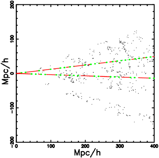
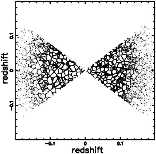
As an example, we fix attention on the Eso Slice Project (ESP) which covers a strip of 22(RA) $\times$ 1(DE) square degrees, see Vettolani et al. (1998). On the ESP we report two lines over which a random distribution of chords follows the NPVT equation (31) with $b=42.32h^{-1}$ Mpc and $a=0.36$, see Figure 10.

Figure 10: Cone diagram of ESP galaxies when the $X$ and $Y$ axes are expressed in Mpc and $H_{0}=100$ $\mathrm{\ km\ s}^{-1}\mathrm{\ Mpc}^{-1}$ (the Hubble constant), which means $h$=1. Two lines in different directions are drawn with the lengths of the chords randomly generated with NPVT PDF $g_{NPVT,3}(r;a,b)$ when $b=42.32h^{-1}$ Mpc and $a=0.36$. Each chord has a different color, red and green, and different line styles, full and dotted.

0.4.2 A simulated slice

In order to simulate the 2dF Galaxy Redshift Survey (2dFGRS), we simulate a 2D cut on a 3D PVT network organized in two strips about $75^{\circ}$ long, see Figure 11

Figure 11: Portion of the NPVT $V_{p}(2,3)$; cut on the X-Y plane when two strips of $75^{\circ}$ are considered. The parameters of the simulation, see Zaninetti (2010), are pixels = 1500, side = 131 908 Km/sec and amplify = 1.2. Along a line which crosses the center, the chords between a face and the next one are drawn. Each chord has a different color, red and green, and different line styles, full and dotted. The fraction of volume forbidden to the NPVT seeds is $f=16\%$ and the number of the seeds, 77 730, is chosen in order to have $b=42.32h^{-1}$ Mpc.

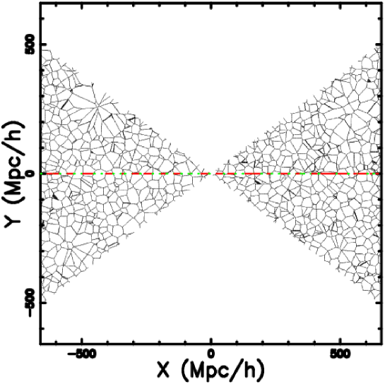
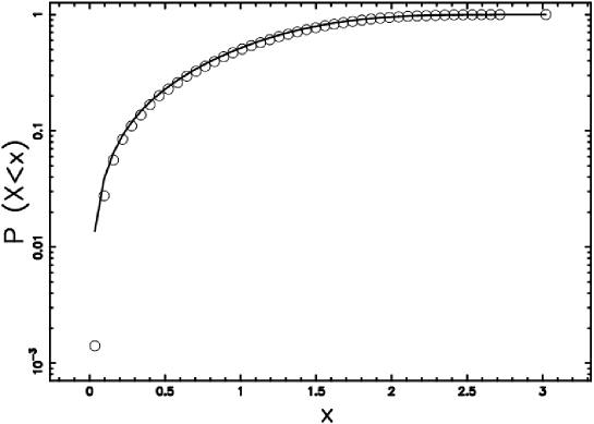
Figure 12 shows a superposition of the numerical frequencies in chord lengths of a 3D PVT simulation with the curve of the theoretical PDF of PVT chords, $g(l,b)$, as given by Eq. (28).

Figure 12: Histogram of the frequencies in chord lengths along 31 lines (1617 sequential chords) with a superposition of the theoretical NPVT PDF as represented by Eq. (31). The number of bins is 30, the reduced $\chi^{2}$ is 9.21, and $b=42.32h^{-1}$ Mpc.

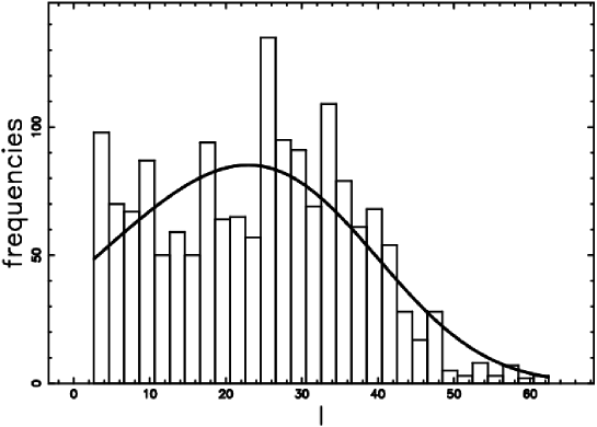
The distribution of the galaxies as given by NPVT is reported in Figure 13, conversely Figure 15 in Zaninetti (2010) was produced with PVT.

Figure 13: Polar plot of the pixels belonging to a slice $75^{\circ}$ long and $3^{\circ}$ wide generated by NPVT seeds. This plot contains 40 000 galaxies, the maximum frequency of theoretical galaxies is at $z=0.056$. In this plot, $\mathcal{M_{\sun}}$ = 5.33 and $h$=1.

0.5 Conclusions

A mathematical method was developed for the chord length distribution obtained from the sphere diameter distribution function which approximates the volume of the PVT. The new chord length distribution as represented by the PVT formula (28) can give mathematical support for the periodicity along a line, or a cone, characterized by a small solid angle. At the same time, a previous analysis has shown that the best fit to the effective radius of the cosmic voids as deduced from the catalog SDSS R7 is represented by a Kiang function with $c\approx 2$. Also in this case we found an expression for the chord length given by the 3D NPVT formula (31). In order to produce this kind of NPVT volumes, a new type of seed has been introduced, see Section 0.3.3. These new seeds are also used to simulate the intersection between a plane and the NPVT network. A careful choice of the number of seeds allows matching the simulated value of the scaling $b$ with the desired value of $b=42.32h^{-1}$ Mpc, see Figure 12.

References

- Bell & McDiarmid (2006) Bell, M. B., & McDiarmid, D. 2006, ApJ , 648, 140
- Broadhurst et al. (1990) Broadhurst, T. J., Ellis, R. S., Koo, D. C., & Szalay, A. S. 1990, Nature , 343, 726
- Ferenc & Néda (2007) Ferenc, J.-S., & Néda, Z. 2007, Phys. A , 385, 518
- Hartnett (2009a) Hartnett, J. G. 2009a, in Astronomical Society of the Pacific Conference Series, Vol. 413, 2nd Crisis in Cosmology Conference, ed. F. Potter, 77
- Hartnett (2009b) Hartnett, J. G. 2009b, Astrophysics and Space Science , 324, 13
- Kiang (1966) Kiang, T. 1966, Z. Astrophys. , 64, 433
- Okabe et al. (2000) Okabe, A., Boots, B., Sugihara, K., & Chiu, S. 2000, Spatial Tessellations. Concepts and Applications of Voronoi Diagrams, 2nd ed. (Chichester, New York: Wiley)
- Pan et al. (2012) Pan, D. C., Vogeley, M. S., Hoyle, F., Choi, Y.-Y., & Park, C. 2012, MNRAS , 421, 926
- Ruan et al. (1988) Ruan, J. Z., Litt, M. H., & Krieger, I. M. 1988, Journal of Colloid and Interface Science, 126, 93
- Szalay et al. (1993) Szalay, A. S., Broadhurst, T. J., Ellman, N., Koo, D. C., & Ellis, R. S. 1993, Proceedings of the National Academy of Science, 90, 4853
- Tifft (1973) Tifft, W. G. 1973, ApJ , 179, 29
- Tifft (1980) —. 1980, ApJ , 236, 70
- Tifft (1995) —. 1995, Astrophysics and Space Science , 227, 25
- Vettolani et al. (1998) Vettolani, G., Zucca, E., Merighi, R., Mignoli, M., Proust, D., Zamorani, G., Cappi, A., Guzzo, L., Maccagni, D., Ramella, M., Stirpe, G. M., Blanchard, A., Cayatte, V., Collins, C., MacGillivray, H., Maurogordato, S., Scaramella, R., Balkowski, C., Chincarini, G., & Felenbok, P. 1998, A&AS , 130, 323
- Zaninetti (2010) Zaninetti, L. 2010, Revista Mexicana de Astronomia y Astrofisica, 46, 115
- Zaninetti (2012) —. 2012, Revista Mexicana de Astronomia y Astrofisica, 48, 209