Pauli spin blockade and the ultrasmall magnetic field effect

Abstract

Based on the spin-blockade model for organic magnetoresistance we present an analytic expression for the polaron-bipolaron transition rate, taking into account the effective nuclear fields on the sites. We reveal the physics producing qualitatively different magnetoconductance line shapes as well as the ultrasmall magnetic field effect, and we study the role of the ratio between the intersite hopping rate and the typical magnitude of the nuclear fields. Our findings are in agreement with recent experiments and numerical simulations.

The discovery some ten years ago of spin injection in organic semiconductors Dediu2002181 and a giant magnetoresistance in organic spin valves kalinowski ; xiong:nature triggered the birth of the thriving field of organic spintronics orgspinrev , which offers interesting new physics and the potential of industrial applications. An exciting phenomenon in this field is a large (up to 20%) magnetoresistance observed in different organic materials francis-njp-2004 ; PhysRevB.72.205202 ; PhysRevLett.99.257201 , usually at small magnetic fields (1–10 mT) but sometimes at larger fields (10–100 mT), and persisting up to room temperature. Since its discovery in 2004, different explanations for this organic magnetoresistance (OMAR) have been proposed: For bipolar devices it was suggested that spin-dependent electron-hole recombination and dissociation rates could be responsible Prigodin2006757 ; PhysRevB.76.235202 , whereas a model based on nuclear-field-mediated bipolaron formation could explain OMAR in both bipolar and unipolar devices PhysRevLett.99.216801 ; wagemansjap ; PhysRevB.84.075204 .

More recently an organic magnetoresistive effect on an even smaller field scale (0.1–1 mT) has been observed in unipolar as well as bipolar devices PhysRevLett.105.166804 . This ultrasmall magnetic field effect (USMFE) is manifested by a sign reversal of the magnetoconductance (MC) at very small fields, creating two small peaks(dips) around zero field for devices with a negative(positive) MC. Experimental results seem to indicate that the typical field magnitude on which the USMFE is observed scales with the width of the MC curve when different materials are investigated PhysRevLett.105.166804 . An explanation for the effect was suggested in terms of enhanced singlet-triplet mixing close to the crossings of the hyperfine sublevels of pairs of charge carriers (polarons) coupled to single nuclear spins nguyennatmat . This explanation is still under debate, mainly because it is expected that a single polaron in reality couples to many nuclear spins McCamey ; bobbertnatmat ; schultenspin . Numerical simulations based on a semiclassical model (where the coupling to an ensemble of nuclear spins is treated as an effective magnetic field) also reproduce the USMFE PhysRevLett.106.197402 and thus invite to seek for an explanation along semiclassical lines.

Here, we study the OMAR line shape as it naturally emerges from the spin blockade model of Ref. PhysRevLett.99.216801 . We present an analytic expression for the charge current through a polaron-bipolaron link for a given realization of the nuclear fields. Our results reproduce the USMFE and the different line widths as observed in experiment and in numerical calculations based on the same semiclassical approach PhysRevLett.106.197402 , and from our analytic insight we can identify the underlying physical mechanisms. We note that many interesting aspects of spin-blockade physics have already been investigated in the seemingly foreign field of spin qubits hosted in semiconductor quantum dots ono:science ; jouravlev:prl , where spin blockade is commonly used as a tool for single-qubit readout frank:nature ; reillyt2 . Indeed, the physics of the polaron spin blockade model for OMAR is very similar to that governing the electron transport through a double quantum dot in the spin-blockade regime jouravlev:prl . Our investigation thus builds on the theoretical framework of Ref. jouravlev:prl , and our explanation of the USMFE relies on a subtlety which was not addressed in Ref. jouravlev:prl .

Let us first briefly review the bipolaron model for OMAR presented in Ref. PhysRevLett.99.216801 . Electric current flows through the organic material as polarons hop between different localized molecular sites. Typically, the sites participating in transport do not form a regular lattice and all have a random energy offset with a distribution width $\sigma$ of 0.1–0.2 eV PhysRevLett.99.216801 . Sites with a relatively large negative energy offset are likely to trap a polaron for a long time, but since the on-site polaron-polaron repulsion is typically of the same order of magnitude as $\sigma$, such occupied sites can often still take part in transport by temporarily hosting a pair of polarons, i.e. a bipolaron.

Due to a relatively large orbital level spacing, most energetically accessible bipolaron states are spin singlets. This makes the polaron-bipolaron transition spin selective, ultimately leading to OMAR. The mechanism can be understood from Fig. 1, where we focus on a single polaron-bipolaron transition. We assume that the spins of the two encountering polarons are random and for simplicity we describe the problem in the basis of spin eigenstates quantized along the direction of the local magnetic fields ${\bf B}_{L,R}$. Two possible initial spin states are depicted: (i) the left spin antiparallel and the right spin parallel to the local field, and (ii) both spins parallel. In the absence of an external field, the magnetic fields at the two sites are the local random effective nuclear fields [Fig. 1(a)]. Generally all initial states can then transition to a spin-singlet bipolaron and current runs through the system. If, on the other hand, a magnetic field much larger than the typical nuclear fields is applied, then ${\bf B}_{L}$ and ${\bf B}_{R}$ are (almost) parallel [Fig. 1(b)]. In this case, situation (ii) is a spin triplet, out of which a bipolaron cannot be formed: the current is blocked.

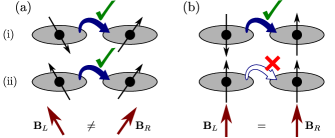
Figure 1: (color online) When a site has a relatively large negative energy offset and already contains a polaron (the right site in the pictures), charge transport through this site relies on the formation of a bipolaron (blue arrows). Large on-site exchange effects dictate this bipolaron to be a spin-singlet, which leads to spin-blockade physics.

We thus see that a simple two-site picture is able to explain the essentials of OMAR. Of course, in experiment there are many possible paths for charge carriers through the material and not all of them contain bipolaron sites. The visibility of all effects of spin blockade will thus be reduced, but the characteristic features survive PhysRevLett.99.216801 .

In this work, we will focus on the physics of a single polaron-bipolaron transition and its MC line shape. To describe the transition, we use five states: the four possible initial spin states of the polaron pair (both sites hosting one polaron), one spin-singlet state $\left|S\right\rangle$ and three spin-triplet states $\left|T_{0}\right\rangle$ and $\left|T_{\pm}\right\rangle$, and the spin-singlet bipolaron state $\left|S_{\rm b}\right\rangle$. The Hamiltonian we use to describe the coherent dynamics of these states reads jouravlev:prl

$$\hat{H}=\left(\begin{array}[]{ccccc}B_{s}^{z}&B_{s}^{-}&0&-B_{a}^{-}&0\\ B_{s}^{+}&0&B_{s}^{-}&B_{a}^{z}&0\\ 0&B_{s}^{+}&-B_{s}^{z}&B_{a}^{+}&0\\ -B_{a}^{+}&B_{a}^{z}&B_{a}^{-}&0&t\\ 0&0&0&t&-\Delta\\ \end{array}\right),$$ (1)

written in the basis $\{\left|T_{+}\right\rangle,\left|T_{0}\right\rangle,\left|T_{-}\right\rangle,\left|S\right\rangle,\left|S_{\rm b}\right\rangle\}$. This Hamiltonian includes a coupling energy $t$ between the two singlets (which enables polaron hopping) and the relative energy offset (detuning) $\Delta$ of the bipolaron state, typically $\Delta\sim\sigma$. The effect of the local magnetic fields ${\bf B}_{L,R}$ is expressed in terms of the sum and difference fields ${\bf B}_{s}=\tfrac{1}{2}({\bf B}_{L}+{\bf B}_{R})$ and ${\bf B}_{a}=\tfrac{1}{2}({\bf B}_{L}-{\bf B}_{R})$, and we use the notation $B_{s(a)}^{\pm}=\tfrac{1}{\sqrt{2}}(B_{s(a)}^{x}\pm iB_{s(a)}^{y})$. Note that we have set $g\mu_{\rm B}=1$ for convenience.

As pointed out in Ref. jouravlev:prl , we can deduce already from Eq. (1) that there exist in the space of $({\bf B}_{L},{\bf B}_{R})$ so-called “stopping points” where the current is blocked. To see this, we take the spin quantization axis to point along ${\bf B}_{s}$, which amounts to setting $B_{s}^{\pm}\to 0$ in (1). Then we find that current vanishes when ${\bf B}_{a}\parallel{\bf B}_{s}$ or ${\bf B}_{a}\perp{\bf B}_{s}$, since at these points one or more of the triplet states are not coupled to $\left|S\right\rangle$. The sum and difference fields ${\bf B}_{s,a}$ both contain a contribution from the effective nuclear fields ${\bf K}_{L,R}$ on the two sites, whereas the external field ${\bf B}_{\rm ext}$ only adds to the sum field: ${\bf B}_{s}={\bf K}_{s}+B_{\rm ext}\hat{z}$ and ${\bf B}_{a}={\bf K}_{a}$. For a given random realization of ${\bf K}_{L,R}$ one can thus always find a field $B_{\rm ext}$ for which ${\bf B}_{a}\perp{\bf B}_{s}$, and a sweep of $B_{\rm ext}$ for a fixed ${\bf K}_{L,R}$ will always exhibit a stopping point where the current vanishes. The position of this stopping point is determined by the relative orientation of ${\bf K}_{s}$ and ${\bf K}_{a}$ and is thus random. In an experiment one usually sweeps $B_{\rm ext}$ so slowly that at each measurement many configurations of the fields ${\bf K}_{L,R}$ are probed. As a result the stopping points are averaged out and one finds a smooth MC curve jouravlev:prl .

However, this is not the full story. A subtlety, not discussed in Ref. jouravlev:prl , is that there exists one more stopping point omar.note1 : When ${\bf B}_{s}=0$ the triplet subspace in the Hamiltonian is degenerate and Eq. (1) can be equivalently written in terms of one coupled triplet state

$$\left|T_{m}\right\rangle=\frac{-B_{a}^{-}\left|T_{+}\right\rangle+B_{a}^{z}\left|T_{0}\right\rangle+B_{a}^{+}\left|T_{-}\right\rangle}{|{\bf B}_{a}|},$$

and two orthogonal triplet states $\left|T_{1}\right\rangle$ and $\left|T_{2}\right\rangle$ which have $\mathinner{\langle{T_{1,2}|\hat{H}|S}\rangle}=0$ and are thus blocked. Why would we bother? We argued above that stopping points occur at random positions, leaving no trace after averaging over ${\bf K}_{L,R}$. This new stopping point however, is fundamentally different from the ones discussed above: It suppresses current close to where ${\bf B}_{\rm ext}=-{\bf K}_{s}$, which is always in the vicinity of $B_{\rm ext}=0$. It is therefore possible that after averaging over ${\bf K}_{L,R}$ this new stopping point leaves a trace in the MC curve: A small dip around zero field, like the USMFE.

Let us now explicitly calculate the current as governed by this polaron-bipolaron transition. To describe charge transport, we write a time-evolution equation for the $5\times 5$ density matrix of the system. To the coherent evolution dictated by $\hat{H}$ we add incoherent rates describing dissociation of the bipolaron to the environment and hopping of a new polaron onto the empty left site. This yields (where we have set $\hbar$ to $1$)

$$\frac{\partial\hat{\rho}}{\partial t}=-i[\hat{H},\hat{\rho}]-\frac{\Gamma}{2}\{\hat{P}_{\rm b},\hat{\rho}\}+\frac{\Gamma}{4}\rho_{{\rm b},{\rm b}}(1-\hat{P}_{\rm b})\hat{\mathbbm{1}},$$ (2)

where $\Gamma$ is the rate of bipolaron dissociation to the environment, $\hat{P}_{\rm b}=\left|S_{\rm b}\right\rangle\left\langle S_{\rm b}\right|$ is the projection operator onto the bipolaron state, and $\hat{\mathbbm{1}}$ is the identity matrix. In writing so we assumed for simplicity that refilling of the left site takes place immediately after dissociation of the bipolaron. If this is not the case, the prefactor for the current changes but the MC characteristics stay the same.

We add the normalization condition ${\rm Tr}[\hat{\rho}]=1$ to the set of equations and then solve $\partial_{t}\hat{\rho}^{({\rm eq})}=0$ to find the stationary density matrix. The charge current is then given by $I=e\Gamma\rho^{({\rm eq})}_{{\rm b},{\rm b}}$ and can be found explicitly. We assume for convenience that $\Gamma\gg t,B_{s},B_{a},\Delta$ is the largest energy scale in the problem PhysRevB.84.075204 , and then find

$$I=e\Gamma_{s}\frac{4x^{2}\sin^{2}\phi}{x^{4}+ax^{2}+1},$$ (3)

in terms of $x\equiv B_{s}/B_{a}$. Here $\Gamma_{s}\equiv t^{2}/\Gamma$ is the singlet-singlet hopping rate from the left to the right site and $\phi$ is the angle between ${\bf B}_{s}$ and ${\bf B}_{a}$ omar.note2 . We also used

$$a=\frac{\Gamma_{s}^{2}}{B_{a}^{2}}\left(3+\frac{1}{\cos^{2}\phi}\right)-2\cos 2\phi.$$ (4)

We see that all stopping points predicted above are indeed reflected in (3): At $B_{s}=0$ we have $x=0$ which yields $I=0$, and ${\bf B}_{a}\parallel{\bf B}_{s}$ or ${\bf B}_{a}\perp{\bf B}_{s}$ corresponds to $\phi=0,\pi$ or $\phi=\pi/2$ respectively, both also giving $I=0$.

Equation (3) is the most important analytic result of our work. It gives the current for one single realization of ${\bf K}_{L}$, ${\bf K}_{R}$, and $B_{\rm ext}$. The MC measured in experiment is found by averaging (3) over the random nuclear fields. In contrast to the analytic results presented in jouravlev:prl , our result is valid for arbitrary $\Gamma_{s}$ and not only for limiting cases. One word of caution is required here concerning the interpretation of (3): If one wants to plot $I(B_{\rm ext})$ for a single realization of ${\bf K}_{L,R}$, one should not only use $B_{s}=|{\bf K}_{s}+B_{\rm ext}\hat{z}|$ in (3) but also implement the dependence of $\phi$ on $B_{\rm ext}$ implied by $\cos\phi=({\bf B}_{s}\cdot{\bf B}_{a})/B_{s}B_{a}$.

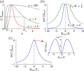
Figure 2: (color online) (a) The current given by (3) as a function of $x=B_{s}/B_{a}$ for fixed $B_{a}$ and $\phi$, evaluated for different parameters $a$. (b,c) The averaged MC. (b) Blue trace: $\Gamma_{s}/K\ll 1$. The field $B_{\rm ext}$ is plotted in units of $K=\langle{K}^{2}_{L,R}\rangle^{1/2}$. The peak of this curve is flat jouravlev:prl . Green trace: $\Gamma_{s}/K=\tfrac{3}{2}$. (c) $\Gamma_{s}/K=50$. Now $B_{\rm ext}$ is plotted in units of $\Gamma_{s}$. (inset) The range where $B_{\rm ext}\sim K$.

Let us now investigate Eq. (3) and see what we can infer about the line shape of the predicted MC curve. We always have $a>-2$, which ensures that $I\geq 0$ everywhere. The current vanishes for $x=0$ or $x\to\infty$, and in the range $x\in[0,\infty]$ we have a single maximum at $x=1$ where the current is $I_{\rm max}=4e\Gamma_{s}\sin^{2}\phi/(a+2)$. In Fig. 2(a) we plot the expression given in Eq. (3) for different $a$. The FWHMs $w_{-}$ of the dip around $x=0$ and $w_{+}$ of the overall peak structure (as indicated in the plot for $a=4$) are found to be $w^{2}_{\pm}=2+\tfrac{1}{2}a\pm\sqrt{3+2a+\tfrac{1}{4}a^{2}}$.

We see from Eq. (4) that an important parameter is $\Gamma_{s}/K$, the ratio of the intersite hopping rate and the typical magnitude of the nuclear fields $K$, typically $\sim 0.1~{}\mu$eV McCamey . We will thus now investigate the cases of small and large $\Gamma_{s}/K$.

In the limit of $\Gamma_{s}/K\ll 1$ we can write

$$I\approx e\Gamma_{s}\frac{4x^{2}\sin^{2}\phi}{x^{4}-2x^{2}\cos 2\phi+1}=\Gamma_{s}({\bf n}_{L}\times{\bf n}_{R})^{2},$$ (5)

where we used the unit vectors ${\bf n}_{L,R}={\bf B}_{L,R}/B_{L,R}$. As it should, this result coincides with that of Ref. jouravlev:prl in the same limit: There are no intersite exchange effects and the situation is exactly like the picture of Fig. 1 where the current only depends on the relative orientation of ${\bf B}_{L}$ and ${\bf B}_{R}$. As was shown in jouravlev:prl , Eq. (5) can be averaged analytically over random ${\bf K}_{L,R}$ taken from a normal distribution, yielding a MC curve with a flat peak at $B_{\rm ext}=0$, a maximum of $\langle I\rangle_{\rm max}\sim e\Gamma_{s}$, and a line width of $\sim K$. Indeed, for all $a\in[-2,2]$ we find that $w_{+}\sim 1$, so for any $\phi$ the current is suppressed when $x\gtrsim 1$. In Fig. 2(b) (blue trace) we plot the resulting MC line shape, where we defined $MC(B_{\rm ext})=[I(B_{\rm ext})-I(0)]/I(0)$.

In the opposite limit of $\Gamma_{s}/K\gg 1$ we have $a\approx(\Gamma_{s}/B_{a})^{2}(3+\cos^{-2}\phi)\gg 1$. We can already see from the properties of Eq. (3) that in this case $\langle I\rangle_{\rm max}\sim eK^{2}/\Gamma_{s}$, and that $w_{+}\approx a^{1/2}\sim\Gamma_{s}/K$ implies a MC line width of $\sim\Gamma_{s}$. Indeed, $\Gamma_{s}$ sets the level broadening of $\left|S\right\rangle$ and as long as $B_{s}\lesssim\Gamma_{s}$ generally all three triplet states can efficiently transition to $\left|S\right\rangle$ with the coupling provided by ${\bf B}_{a}$. The width of the dip around the stopping point at $x=0$ is $w_{-}\approx a^{-1/2}\sim K/\Gamma_{s}$ in terms of $x$, or $\sim K^{2}/\Gamma_{s}$ in terms of $B_{s}$. This energy scale can also be understood: If $B_{s}=0$ the decay rate of $\left|T_{m}\right\rangle$ is $\Gamma_{t}\sim K^{2}/\Gamma_{s}$, which is the only energy relevant in the triplet subspace. When $B_{s}\gtrsim\Gamma_{t}$ the decay of the other two triplet states becomes comparable to $\Gamma_{t}$ and the blockade is lifted.

In this limit of large $\Gamma_{s}/K$ the current cannot be averaged analytically over the nuclear fields, and one has to evaluate the integrals over the distribution of ${\bf K}_{L,R}$ numerically. Fig. 2(c) shows a plot of the MC integrated over normal distributions for all six components of ${\bf K}_{L}$ and ${\bf K}_{R}$. For all components we used a standard deviation of $K/\sqrt{3}$ and we have set $\Gamma_{s}/K=50$. The resulting line shape is Lorentzian since it is determined by the level broadening of $\left|S\right\rangle$. Close to zero field, where $B_{\rm ext}\sim K$, we find a very faint USMFE, as shown in the inset. When we set $\Gamma_{s}/K$ even larger we find that the visibility of this USMFE is suppressed further, ultimately reaching zero.

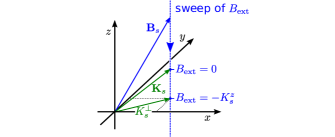
Figure 3: When $B_{\rm ext}$ is swept for a given realization of ${\bf K}_{L,R}$, the field ${\bf B}_{s}$ (blue arrow) follows a trace like the blue dashed line. We indicated with green arrows ${\bf K}_{s}$ as well as $K_{s}^{\perp}$, which equals the minimum value of $B_{s}$.

We can understand this USMFE from the expression for the current given in Eq. (3). For a given realization of ${\bf K}_{L,R}$, the current trace $I(B_{\rm ext})$ “misses” the zero-field stopping point by $K_{s}^{\perp}=\sqrt{(K_{s}^{x})^{2}+(K_{s}^{y})^{2}}$, as illustrated in Fig. 3. Some realizations have $K_{s}^{\perp}\geq B_{a}$ so that the current trace has a single maximum [see Fig. 2(a)]. Other realizations have $K_{s}^{\perp}<B_{a}$ and the current exhibits a dip at small fields, the position of the dip at $B_{\rm ext}=-K_{s}^{z}$. For large $\Gamma_{s}/K$ the dip around the zero-field stopping point becomes narrow, of the order $\sim K^{2}/\Gamma_{s}\ll K$, and only the very few curves of $I(B_{\rm ext})$ with $K_{s}^{\perp}\lesssim K^{2}/\Gamma_{s}$ have an appreciable dip. This still can produce a faint dip in the averaged current. However, the position of each single-realization narrow dip is at $B_{\rm ext}=-K_{s}^{z}$, so averaging over $K_{s}^{z}$ makes the averaged dip even less pronounced and results in a dip width of $\sim K$.

The regime to look for a pronounced USMFE is thus at intermediate $\Gamma_{s}/K\sim 1$. In Fig. 2(b) (green trace) we plot the averaged MC for $\Gamma_{s}/K=3/2$ and we see indeed a strong USMFE, its visibility being $\sim 5$%. This regime is optimal for the USMFE since here the width of the zero-field dip is still $\sim K$ but the symmetric situation where the current only depends on the angle between ${\bf n}_{L}$ and ${\bf n}_{R}$ is significantly perturbed. In other words, at $\Gamma_{s}/K\to 0$ the overall MC line width is minimal and $\sim K$. The two USMFE “bumps” are still there but are split by the same energy scale $\sim K$ and thus appear just left and right of the top of the MC curve. In the limit of $\Gamma_{s}/K=0$ the bumps and the underlying MC curve have exactly compatible shape line shapes, together resulting in the characteristic flat peak. If one moves away from $\Gamma_{s}/K=0$ the underlying MC line shape becomes broader, which makes the USMFE bumps more visible. However, as soon as $\Gamma_{s}/K$ becomes too large, one enters the regime discussed above, where the USMFE disappears again. The optimal regime is thus at $\Gamma_{s}/K\sim 1$, in agreement with the results presented in Fig. 2(b,c) as well as with previously obtained numerical results PhysRevB.84.075204 .

To summarize, we studied the two-site spin-blockade model for OMAR and derived an analytic expression for the polaron-bipolaron transition rate, taking into account the local nuclear fields on the two sites. We showed how our result reproduces different MC line widths: $\sim K$ for slow and $\sim\Gamma_{s}$ for fast intersite hopping. We also provided an explanation of the USMFE in terms of a persistent spin blockade at the special point where the average effective field vanishes $B_{s}=0$. The USMFE as predicted here always takes place on the field scale $\sim K$, and we explained why it is expected to be most pronounced in the regime where $\Gamma_{s}\sim K$. In this regime thus both the scale of the USMFE and the MC line width are set by $K$, the latter however being slightly larger. This relation between the two scales is consistent with experimental observations PhysRevLett.105.166804 and numerical simulations PhysRevB.84.075204 .

As a side remark we note here that a close inspection of the experimental data presented in Ref. jouravlev:prl (the current through a double quantum dot) also seems to reveal a faint USMFE. The data were fitted to the flat-peak curve since the system was assumed to be in the inelastic tunneling regime. In reality the coupling is however never perfectly inelastic, and a faint trace of the USMFE could be left. Due to its tunability, a double quantum dot might in fact be the best system to experimentally explore USMFE in more detail.

We acknowledge helpful feedback from M. S. Rudner and P. A. Bobbert.

References

- (1) V. Dediu, M. Murgia, F. Matacotta, C. Taliani, and S. Barbanera, Solid State Commun. 122, 181 (2002).
- (2) J. Kalinowski, M. Cocchi, D. Virgili, P. Di Marco, V. Fattori Chem. Phys. Lett. 380, 710 (2003).
- (3) Z. H. Xiong, D. Wu, Z. Valy Vardeny, and J. Shi, Nature (London) 427, 821 (2004).
- (4) V. A. Dediu, L. E. Hueso, I. Bergenti, and C. Taliani, Nat. Mater. 8, 707 (2009).
- (5) T. L. Francis, Ö. Mermer, G. Veeraraghavan, and M. Wohlgenannt, New Journal of Physics 6, 185 (2004).
- (6) Ö. Mermer, G. Veeraraghavan, T. L. Francis, Y. Sheng, D. T. Nguyen, M. Wohlgenannt, A. Köhler, M. K. Al-Suti, and M. S. Khan, Phys. Rev. B 72, 205202 (2005).
- (7) F. L. Bloom, W. Wagemans, M. Kemerink, and B. Koopmans, Phys. Rev. Lett. 99, 257201 (2007).
- (8) V. Prigodin, J. Bergeson, D. Lincoln, and A. Epstein, Synthetic Metals 156, 757 (2006).
- (9) P. Desai, P. Shakya, T. Kreouzis, and W. P. Gillin, Phys. Rev. B 76, 235202 (2007).
- (10) P. A. Bobbert, T. D. Nguyen, F. W. A. van Oost, B. Koopmans, and M. Wohlgenannt, Phys. Rev. Lett. 99, 216801 (2007).
- (11) W. Wagemans, F. L. Bloom, P. A. Bobbert, M. Wohlgenannt, and B. Koopmans, J. Appl. Phys. 103, 07F303 (2008).
- (12) A. J. Schellekens, W. Wagemans, S. P. Kersten, P. A. Bobbert, and B. Koopmans, Phys. Rev. B 84, 075204 (2011).
- (13) T. D. Nguyen, B. R. Gautam, E. Ehrenfreund, and Z. V. Vardeny, Phys. Rev. Lett. 105, 166804 (2010).
- (14) T. D. Nguyen, G. Hukic-Markosian, F. Wang, L. Wojcik, X.-G. Li, E. Ehrenfreund, and Z. V. Vardeny, Nat. Mater. 9, 345 (2010).
- (15) D. R. McCamey, K. J. van Schooten, W. J. Baker, S.-Y. Lee, S.-Y. Paik, J. M. Lupton, and C. Boehme Phys. Rev. Lett. 104, 017601 (2010).
- (16) P. A. Bobbert, Nat. Mater. 9, 288 (2010).
- (17) K. Schulten and P. G. Wolynes, J. Chem. Phys. 68, 3292 (1978).
- (18) S. P. Kersten, A. J. Schellekens, B. Koopmans, and P. A. Bobbert, Phys. Rev. Lett. 106, 197402 (2011).
- (19) K. Ono, D. G. Austing, Y. Tokura, and S. Tarucha, Science 297, 1313 (2002).
- (20) O. N. Jouravlev and Y. V. Nazarov, Phys. Rev. Lett. 96, 176804 (2006).
- (21) F. H. L. Koppens, C. Buizert, K. J. Tielrooij, I. T. Vink, K. C. Nowack, T. Meunier, L. P. Kouwenhoven, and L. M. K. Vandersypen, Nature 442, 766 (2006).
- (22) D. J. Reilly, J. M. Taylor, J. R. Petta, C. M. Marcus, M. P. Hanson, and A. C. Gossard, Science 321, 817 (2008).
- (23) One could argue that is also a stopping point, but it is not of any interest since it occurs independently from and therefore leaves no traces in the MC curve. In that sense it is also not really a stopping point. Besides, it is captured by the model in jouravlev:prl since it is equivalent to having and .
- (24) If one would relax the assumption , one finds the same expression but with and an extra prefactor . A finite detuning thus merely leads to a suppression of the current as well as a smaller effective hopping rate.