Equation of State within Gluon Dominated QGP Model in Relativistic Hydrodynamics Approach

Abstract

The dynamics of Quark-gluon plasma (QGP) as a lump of deconfined free quarks and gluons is elaborated. Based on the first principal we construct the Lagrangian that represents the dynamics of QGP. To induce a hydrodynamics approach, we substitute the gluon fields with flow fields. As a result, the derived equation of Motion (E.O.M) for gluon dominated QGP shows the form that similar to Euler equation, and the energy momentum tensor also represents explicitly the system of ideal fluid. Combining the E.O.M and energy momentum tensor, the pressure and energy density distribution as the equation of states are analytically derived.

1 Introduction

Recent experiments on heavy-ion collisions show a strong indication that hot dense deconfined phase of free quark and gluon, the so called quark-gluon plasma (QGP), is conjectured to exist. The study of QGP itself has been carried out through a number of different approaches in the previous works. Some results of these studies were obtained in the framework of quantum chromodynamics (QCD) theory by utilizing the lattice gauge calculation [1, 2]. Other calculations of QGP were based on the relativistic hydrodynamics approach [3, 4]. In the latter, the QGP could be either quark [4] or gluon [3] dominated matter. For the quark dominated approach, a very small ratio of shear viscosity over entropy is required to get a good fit of the spectra of transverse momentum, energy density distribution and other physical observables that are obtained from experiments [5, 6, 7, 8, 9, 10]. On the other hand, the gluon dominated plasma motivated by the discoveries of jet quenching in the heavy-ion collision at RHIC indicates the shock waves in the form of Mach cone [11, 12]. The present paper adopts the so-called fluid QCD model [14, 15] to produce the equation of motion and energy momentum tensor for quark and gluon in a lump of QGP, and subsequently to investigate the distribution of the pressure and energy density.

This paper is organized as follows. In Section 2 the fluid QCD model is briefly revisited, and the energy momentum tensor for ideal fluid is derived. Then, it is followed by the derivation for the equation of state and the explicit expression of gluon field in Section 3. Finally, the summary and discussion will be given in Section 4. Throughout this work, we use the natural units, i.e, $\hbar\equiv c\equiv 1$.

2 Model

The Lagrangian of QGP that describes the unification of fermions and bosons from different gauge groups with preserving ${\rm SU}(3)_{F}\otimes{\rm U}(1)_{G}$ gauge symmetry can be written as [13, 14]

$${\cal L}=i\bar{Q}\gamma^{\mu}\partial_{\mu}Q-m_{Q}\bar{Q}Q-{\textstyle\frac{1}{4}}S^{a}_{\mu\nu}S^{a\mu\nu}-{\textstyle\frac{1}{4}}F_{\mu\nu}F^{\mu\nu}+g_{F}J^{a}_{F\mu}U^{a\mu}+g_{G}J_{G\mu}A^{\mu},$$ (1)

where $Q$ and $\bar{Q}$ represent the quark and anti-quark triplet, $\gamma^{\mu}$ is Dirac gamma matrices, and $m_{Q}$ is the mass of quark. The factor ${\textstyle\frac{1}{4}}S^{a}_{\mu\nu}S^{a\mu\nu}$ is the gauge invariant kinetic term of gluon field. The gluon field strength tensor itself is expressed as $S^{a}_{\mu\nu}\equiv\partial_{\mu}U^{a}_{\nu}-\partial_{\nu}U^{a}_{\mu}+g_{F}f^{abc}U^{b}_{\mu}U^{c}_{\nu}$. In the latter, $U^{a}_{\mu}$ indicates the gluon field, $g_{F}$ is the strong coupling constant, and $f^{abc}$ is the structure constant of SU(3) gauge group. The kinetic term for gauge boson $A_{\mu}$ is built inside its field strength tensor, i.e., $F_{\mu\nu}\equiv\partial_{\mu}A_{\nu}-\partial_{\nu}A_{\mu}$. The last two terms of Eq. (1), $J^{a}_{F\mu}=\bar{Q}T^{a}_{F}\gamma_{\mu}Q$ and $J_{G\mu}=\bar{Q}\gamma_{\mu}Q$, represent the quark currents from the SU(3) and U(1) gauge groups, respectively, whereas $g_{G}$ denotes the coupling constant from U(1) gauge group.

The QCD Lagrangian in Eq. (1) is constructed with a purpose to reproduce the energy momentum tensor that has the same form as the energy momentum tensor of an ideal fluid [13]. In the succeeding step, the gluon field $U^{a}_{\mu}$, that is designed to act as the flow field in the system is proposed to be formulated in a configuration that inherently contains the relativistic flow. It is formulated as $U^{a}_{\mu}=(U^{a}_{0},\textbf{U}^{a})\equiv u_{\mu}\phi^{a}$ [14, 15]. Here, $\phi^{a}$ is the dimension one scalar field, and $u_{\mu}\equiv\gamma(1,\textbf{v})$ is the relativistic velocity, with $\gamma=(1-|\textbf{v}|^{2})^{-1/2}$.

This formulation provides a clue that a single gluonic field $U^{a}_{\mu}$ may behaves as a fluid at certain scale, beside its conventional point particle properties with a polarization vector $\epsilon_{\mu}$ in the form of $U^{a}_{\mu}=\epsilon_{\mu}\,\phi^{a}$. One can then consider that there is a kind of “phase transition”,

$$\underbrace{\mathrm{hadronic\;state}}_{\displaystyle\epsilon_{\mu}}\longleftrightarrow\underbrace{\mathrm{QGP\;state}}_{\displaystyle u_{\mu}}.$$

As the gluon field behaves as a point particle, it is in a stable hadronic state and is characterized by its polarization vector. On the other hand in the pre-hadronic state (before hadronization) like hot QGP, the gluon field behaves as a highly energized flow particle and the properties are dominated by its relativistic velocity.

The field $U^{a}_{\mu}$ is actually analogous to the gauge boson from $U(1)$ gauge group in particle physics, where the polarization vector $\epsilon_{\mu}$ from the free photon solution $\sim\epsilon_{\mu}\exp(-ip_{\mu}x^{\mu})$ is replaced by the 4-velocity $u_{\mu}$. Recall that the wavefunction $U^{a}_{\mu}$ for a free particle satisfies $[g^{\mu\nu}(\partial^{2}+m^{2})-\partial^{\nu}\partial^{\mu}]U^{a}_{\mu}=0$ with solution $U^{a}_{\mu}\sim\epsilon_{\mu}\;\phi^{a}\exp(-ip_{\mu}x^{\mu})$. For a massive vector particle, $m\neq 0$, we have no choice but to take $\partial^{\mu}U^{a}_{\mu}=0$. It is not a gauge condition like the case of massless particle. This then demands $p^{\mu}\epsilon_{\mu}=0$. The number of independent polarization vectors is reduced from four to three in a covariant fashion. However, one can still perform another gauge transformation to the massless $U_{\mu}^{a}$ which makes finally only two degrees of freedom remain. Therefore, one should keep in mind that in the present model the spatial velocity has only two degrees of freedom, that means one component must be described by another two vector components.
Further, when Euler-Lagrange equation is applied to Eq. (1) one obtain

$$\frac{\partial}{\partial t}(\gamma\mathbf{v}\phi^{a})+\nabla(\gamma\phi^{a})=-g_{F}\oint d\mathbf{x}(J^{a}_{F0}+F^{a}_{0})~{},$$ (2)

where $J^{a}_{F0}$ denotes the covariant current originating from the quarks that are surrounded by and interact with the gluon ”fluid”, while the term $F^{a}_{\mu}$ is induced by the fluid self-interaction and the interacting gauge fields $A^{a}_{\mu}$. Equation (2) is considered as the general relativistic fluid equation for single gluon field $U^{a}_{\mu}$, since in the non-relativistic limit, i.e. $\phi^{a}\sim 1$ and $\gamma\sim 1+\frac{1}{2}|\mathbf{v}|^{2}$, Eq. (2) transforms to the classical equation of motion of fluid dynamics [14]

$$\frac{\partial\mathbf{v}}{\partial t}+(\mathbf{v}\cdot\nabla)\mathbf{v}=-g_{F}\oint d\mathbf{x}(J^{a}_{F0}+F^{a}_{0})\mid_{\rm non-rel}~{}.$$ (3)

This shows that from a certain point of view the Lagrangian describes a general relativistic fluid system interacting with another gauge field and the matter inside. The flow characteristic that appears in the equation of motion comes from the contribution of gluon field $U^{a}_{\mu}$. This fact indicates that the system we are working with is a gluon dominated QGP. In such system the terms that do not contain gluon field may be omitted. As a consequence we have

$${\cal L} = -{\textstyle\frac{1}{4}}S^{a}_{\mu\nu}S^{a\mu\nu}+g_{F}J^{a}_{F\mu}U^{a\mu}~{}.$$ (4)

The Lagrangian given by Eq. (4) describes the kinetics of gluons, the self-interaction of gluons, the self-interaction between small number of quark and anti-quark, and the interaction between quark with gluon ”fluid”. Electromagnetic interaction also exist in the system, but the scale is suppressed due to its tiny value compared with the strong interaction. From the Lagrangian given in Eq. (4) we can derive the energy momentum tensor [17]

$$\cal{T}_{\mu\nu} = \frac{2}{\sqrt{-g}}\frac{\delta({\cal L}\sqrt{-g})}{\delta g^{\mu\nu}}$$ (5)

$$= S^{a}_{\mu\rho}S^{a\rho}_{\;\;\;\;\nu}-g_{\mu\nu}{\cal L}+2g_{F}J^{a}_{F\mu}U^{a}_{\mu}$$

$$= [2g_{F}g_{\mu\nu}J^{a}_{F\mu}U^{a\mu}+g^{2}_{F}f^{abc}f^{ade}U^{b}_{\mu}U^{c}_{\rho}U^{d\rho}U^{e}_{\nu}]$$

$$-[g_{F}g_{\mu\nu}J^{a}_{F\mu}U^{a\mu}-\frac{1}{4}g_{\mu\nu}g^{2}_{F}f^{abc}f^{ade}U^{b}_{\mu}U^{c}_{\nu}U^{d\mu}U^{e\nu}]~{}.$$

The factor $J^{a}_{F\mu}U^{a\mu}$ in Eq. (5) might be expressed in a more elementary form. To this end, we can start with the assumption that the solution of the Dirac equation for single color quark is in the form of $Q(p,x)=q(p)\exp(-ip\cdot x)$. By inserting this solution to the Dirac equation, i.e., $(i\gamma^{\mu}\partial_{\mu}-m)q(p)\exp(-ip\cdot x)=0$, and multiplying with the anti-quark solution, we obtain $\bar{q}\gamma_{\mu}q=4p_{\mu}$. Since $J^{a}_{F\mu}=\bar{Q}\gamma_{\mu}QT^{a}=\bar{q}\gamma_{\mu}qT^{a}=4p_{\mu}T^{a}$, and $U^{a\mu}=u^{\mu}\phi^{a}$, we finally obtain $J^{a}_{F\mu}U^{a\mu}=4m_{Q}T^{a}\phi^{a}$. Note that we have utilized $u_{\mu}u^{\mu}=1$ along with the assumption that all quarks and anti-quarks have the same momenta $P^{\mu}$ and that the velocities of all gluons and quarks are homogeneous. Thus, the energy momentum tensor in the function of field $\phi^{a}$ reads

$$\cal{T}_{\mu\nu} = [8g_{F}m_{Q}T^{a}\phi^{a}+g^{2}_{F}f^{abc}f^{ade}\phi^{b}\phi^{c}\phi^{d}\phi^{e}]u_{\mu}u_{\nu}$$ (6)

$$-[4g_{F}m_{Q}T^{a}\phi^{a}-\frac{1}{4}g^{2}_{F}f^{abc}f^{ade}\phi^{b}\phi^{c}\phi^{d}\phi^{e}]g_{\mu\nu}~{}.$$

With this form, ${\cal T}_{\mu\nu}$ is obviously describing a system of perfect fluid. Further, we assume that the gluon color states are homogeneous, i.e., $\phi^{a}=\phi$ for all $a=1,\cdots,8$. As the follow-on to this assumption, the generator $T^{a}$ can be compactly written as $T=\sum_{a}T^{a}$ and the 2nd and 4th terms of $\mathcal{T}_{\mu\nu}$ can be omitted due to the completely anti-commutative property of the structure constant $f^{abc}$. The energy momentum tensor then reduces to

$$\cal{T}_{\mu\nu} = (8Tg_{F}m_{Q}\phi)u_{\mu}u_{\nu}-(4Tg_{F}m_{Q}\phi)g_{\mu\nu}$$ (7)

It reveals the collective gluons flow in the system. Therefore, we can temporarily summarize that the system represents an isotropic homogeneous perfect fluid of gluon dominated QGP. Further, to discuss the dynamics of glue lumps, it is also plausible to take the gluon as a field that independent of time, $\phi=\phi(x)$. If we compare Eq.(7) with energy momentum tensor of ideal fluid $\cal{T}_{\mu\nu}=({\cal E}$ $+{\cal P})u_{\mu}u_{\nu}$ - ${\cal P}g_{\mu\nu}$, it becomes obvious that

$${\cal E}={\cal P}=4Tg_{F}m_{Q}\phi.$$ (8)

Here ${\cal P}$ and ${\cal E}$ denote the isotropic pressure and energy density for fluid field, respectively. Or, in currently discussed topic, it is the energy density and pressure distribution in the lump of gluon dominated QGP.

3 Expression for distribution field

The expression for the scalar field $\phi$ can be obtained by deriving the solution of Eq. (3). After applying the assumption of the gluon homogeneity, the equation can be expressed as follow.

$$\delta\partial_{tr}\phi+\gamma\partial_{rr}\phi+\xi+\beta\phi\partial_{t}\phi+\beta\phi\partial_{r}\phi-\lambda\partial_{t}\phi-\lambda\partial_{r}\phi=0,$$ (9)

with $\delta=\gamma|\mathbf{v}|$, $\xi=g_{F}\bar{Q}\gamma_{\mu}TQ$ , $\beta=i\gamma^{2}|\mathbf{v}|^{2}$, $\lambda=(g_{G}/g_{F})A\gamma$, and $\gamma=(1-v^{2})^{-\frac{1}{2}}$. For a simplification but stay relevant, the pressure and energy density distribution of the lump of QGP is assumed to depend only to $r$, it is $\phi=\phi(r)$, and $\partial_{r}\rightarrow d_{r}$. So the term that involve the derivative of $t$ is vanished.

$$\gamma d_{rr}\phi+\beta\phi d_{r}\phi-\lambda d_{r}\phi+\xi=0,$$ (10)

The solution for this equation is

$$\phi = \Big{(}2\gamma\Big{(}\frac{\exp[\frac{r\lambda}{2\gamma}]\Lambda_{1}[x]}{2\gamma}-\frac{\exp[\frac{r\lambda}{2\gamma}]\beta\xi\Lambda_{2}[x]}{2^{1/3}\gamma^{2}(-\frac{\beta\xi}{\gamma^{2}})^{2/3}}$$

$$+\Big{(}\frac{\exp[\frac{r\lambda}{2\gamma}]\Lambda_{3}[x]}{2\gamma}-\frac{\exp[\frac{r\lambda}{2\gamma}]\beta\xi\Lambda_{4}[x]}{2^{1/3}\gamma^{2}(-\frac{\beta\xi}{\gamma^{2}})^{2/3}}\Big{)}C_{2}\Big{)}\Big{)}$$

$$\times 1/\Big{(}\beta\Big{(}\exp[\frac{r\lambda}{2\gamma}]\Lambda_{1}[x]+\exp[\frac{r\lambda}{2\gamma}]\Lambda_{3}[x]C_{2}\Big{)}\Big{)}.$$

When we substitute $\delta,\xi,\beta,\lambda$, and $\gamma$ back to the equation, then $\phi$ appears as

$$\phi = \Big{(}\frac{2}{\sqrt{1-v^{2}}}\Big{(}\frac{\exp[\frac{rgA}{2}]\Lambda_{1}[x]}{2/\sqrt{1-v^{2}}}-\frac{\exp[\frac{rgA}{2}](iv^{2}\xi)^{1/3}\Lambda_{2}[x]}{2^{1/3}}$$ (12)

$$+\Big{(}\frac{\exp[\frac{rgA}{2}]\Lambda_{3}[x]}{2/\sqrt{1-v^{2}}}-\frac{\exp[\frac{rgA}{2}](iv^{2}\xi)^{1/3}\Lambda_{4}[x]}{2^{1/3}}\Big{)}C_{2}\Big{)}\Big{)}$$

$$\times 1/\Big{(}\frac{iv^{2}}{1-v^{2}}\Big{(}\exp[\frac{rgA}{2}]\Lambda_{1}[x]+\exp[\frac{rgA}{2}]\Lambda_{3}[x]C_{2}\Big{)}\Big{)}.$$

Here,

$$\Lambda_{1}[x] = \frac{1}{3^{1/6}\Gamma\big{[}\frac{2}{3}\big{]}}+\frac{3^{1/6}x}{\Gamma\big{[}\frac{1}{3}\big{]}}+\frac{x^{3}}{6\big{(}3^{1/6}\Gamma\big{[}\frac{2}{3}\big{]}\big{)}}+\frac{x^{4}}{4\big{(}3^{5/6}\Gamma\big{[}\frac{1}{3}\big{]}\big{)}}+\mathcal{O}[x]^{5}~{},$$

$$\Lambda_{2}[x] = \frac{3^{1/6}}{\Gamma\big{[}\frac{1}{3}\big{]}}+\frac{x^{2}}{2\big{(}3^{1/6}\Gamma\big{[}\frac{2}{3}\big{]}\big{)}}+\frac{x^{3}}{3^{5/6}\Gamma\big{[}\frac{1}{3}\big{]}}+\frac{x^{5}}{30\big{(}3^{1/6}\Gamma\big{[}\frac{2}{3}\big{]}\big{)}}+\mathcal{O}[x]^{6}~{},$$

$$\Lambda_{3}[x] = \frac{1}{3^{2/3}\Gamma\big{[}\frac{2}{3}\big{]}}-\frac{x}{3^{1/3}\Gamma\big{[}\frac{1}{3}\big{]}}+\frac{x^{3}}{6\big{(}3^{2/3}\Gamma\big{[}\frac{2}{3}\big{]}\big{)}}-\frac{x^{4}}{12\big{(}3^{2/3}\Gamma\big{[}\frac{2}{3}\big{]}\big{)}}+\mathcal{O}[x]^{5}~{},$$

$$\Lambda_{4}[x] = -\frac{1}{3^{1/3}\Gamma\big{[}\frac{1}{3}\big{]}}+\frac{x^{2}}{2\big{(}3^{2/3}\Gamma\big{[}\frac{2}{3}\big{]}\big{)}}-\frac{x^{3}}{3\big{(}3^{1/3}\Gamma\big{[}\frac{1}{3}\big{]}\big{)}}+\frac{x^{5}}{30\big{(}3^{2/3}\Gamma\big{[}\frac{2}{3}\big{]}\big{)}}+\mathcal{O}[x]^{6}~{},$$

and

$$x=\frac{-i2v^{2}(\xi r+\frac{C_{1}}{\sqrt{1-v^{2}}})+g^{2}A^{2}}{2^{4/3}(-iv^{2}\xi)^{2/3}}$$

So far this non-trivial solution is well expressed. But to have a firm solution, some adjustment still need to be carry out at the future works. While for the rest, we will explore the expression for pressure and energy density in the system of gluon dominated quark-gluon plasma.

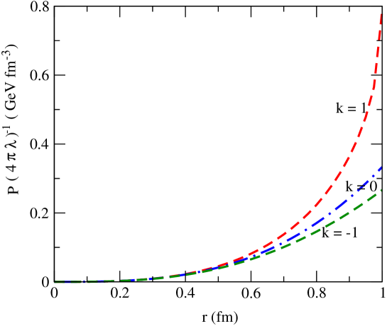
Figure 1: Pressure inside QGP-lump in the function of radius

4 Summary and Discussion

Return to Eq. (8), ${\cal E}={\cal P}=4Tg_{F}m_{Q}\phi$, the energy and pressure can be expressed as follows [16]

$$\rho=P=\int\mathcal{E}d^{4}x=\int{\cal P}d^{4}x=4Tg_{F}f_{Q}m_{Q}\int\int\phi dtdV~{},$$ (13)

where $\mathcal{E}$ and $\mathcal{P}$ denote the isotropic pressure and density for single fluid field, respectively.
By adopting FRW geometry as the background and do integration on the spatial dimension, Eqs. (13) read

$$\rho=P=4\pi\lambda\int R^{3}\phi dt\int\frac{r^{2}dr}{\sqrt{1-kr^{2}}}.$$ (14)

Here we have used $dV={(R^{3}r^{2}sin\theta)}/{\sqrt{1-kr^{2}}}drd\theta d\vartheta$, and $\lambda=4Tg_{F}f_{Q}m_{Q}$. Further, if we assign $\int^{2\pi}_{0}\int^{\pi}_{0}\int dV=4\pi\int\frac{r^{2}dr}{\sqrt{1-kr^{2}}}$ as $\zeta$, then the expression for $P$ and $\rho$ can be written as

$$P=\rho=\lambda\zeta\int R^{3}\phi dt.$$ (15)

In a case when $r$ is constant, $p=\rho\propto\phi(t)dt$, and also if $\phi(t)\propto 1/t$, Then one arrive at $P=\rho\propto\lambda\zeta R^{3}/t$. It indicates that the pressure and energy in the system decrease asymptotically following the increases of time.
Figure 1 shows the total pressure inside the QGP-lump as the function of radius. It is drawn for the simplest condition, where $\phi$ is assumed as a constant, and the scale factor $R=1$. While $k=1,0,-1$ represent the space-time curvature that describe the close, flat, or open space-time that analogous to the close, flat, or open universe. One of the obvious property that appears here is the equation of state $P/\rho=1$. Such a ratio can indicates that in this model the QGP exist within radiation state. This estimate comes from the fact that in general the prerequisite condition for the radiation state is $P\sim 1/3\rho$, and $P/\rho$ is getting smaller along the transition from radiation state to matter state.

Finally, the study revealed observables which should be accessible through heavy ion collisions experiments at the RHIC and LHC. With currently proposed calculation results, such experiments are in future expected to become a reference for adjustments and verifications of the dynamics theory of macroscopic behavior of QGP.

5 References

References

• [1] Gottlieb S 2007 J. Phys. Conf. Ser.  78, 012023
• [2] Petreczky P 2008 Eur. Phys. J.  ST 155, 123
• [3] Bouras I, Molnar E, Niemi H, Xu Z, El A, Fochler O, Greiner C, Rischke D H 2009 Phys. Rev. Lett.  103, 032301
• [4] Romatschke P 2010 Int. J. Mod. Phys. E 19, 1
• [5] Teaney D, Lauret J, Shuryak E V 2001 Phys. Rev. Lett.  86, 4783
• [6] Huovinen P, Kolb P F, Heinz U W, Ruuskanen P V, Voloshin S A 2001 Phys. Lett. B 503, 58
• [7] Kolb P F, Heinz U W, Huovinen P, Eskola K J, Tuominen K 2001 Nucl. Phys. A 696, 197
• [8] Kolb P F, Rapp R 2003 Phys. Rev. C 67, 044903
• [9] Hirano T, Tsuda K 2002 Phys. Rev. C 66, 054905
• [10] Baier R, Romatschke P 2007 Eur. Phys. J. C 51, 677 (2007).
• [11] Adams J et al. 2003 Phys. Rev. Lett.  91, 172302
• [12] Adare A et al. 2008 Phys. Rev. Lett.  101, 232301
• [13] Djun T P, Handoko L T, Soegijono B, Mart T 2015 Int. J. Mod. Phys. A 30 1550077
• [14] Sulaiman A, Fajarudin A, Djun T P, Handoko L T 2009 Int. J. Mod. Phys. A 24, 3630
• [15] Djun T P, Handoko L T 2010 in Proceeding of the Conference in Honor of Murray Gell-Mann’s 80th Birthday: Quantum Mechanics, Elementary Particles, Quantum Cosmology & Complexity, edited by H. Fritzsch and K. K. Phua (Nanyang Technological University, Singapore) , p. 419 arXiv:1109.6066 [hep-ph].
• [16] Nugroho C S, Latief A O, Djun T P, Handoko L T 2012 Grav. Cosmol. 18, 32
• [17] Hobson M P, Efstathiou G, and Lasenby A N (Cambridge University Press 2006) General Relativity