UAB-FT/732
LPT-ORSAY/13-24
MITP/13-020
Optimizing the basis of observables
in the full kinematic range
Sébastien Descotes-Genona, Tobias Hurthb, Joaquim Matiasc
and Javier Virtoc
a Laboratoire de Physique Théorique, CNRS/Univ. Paris-Sud 11 (UMR 8627)
91405 Orsay Cedex, France
b PRISMA Cluster of Excellence & Institute for Physics (THEP)
Johannes Gutenberg University, D-55099 Mainz, Germany
c Universitat Autònoma de Barcelona, 08193 Bellaterra, Barcelona, Catalonia
Abstract
We discuss the observables for the decay, focusing on both CP-averaged and CP-violating observables at large and low hadronic recoil with special emphasis on their low sensitivity to form-factor uncertainties. We identify an optimal basis of observables that balances theoretical and experimental advantages, which will guide the New Physics searches in the short term. We discuss some advantages of the observables in the basis, and in particular their improved sensitivity to New Physics compared to other observables. We present predictions within the Standard Model for the observables of interest, integrated over the appropriate bins including lepton mass corrections. Finally, we present bounds on the S-wave contribution to the distribution coming from the decay, which will help to establish the systematic error associated to this pollution.
1 Introduction
The recent results gathered by the B-factories and the LHCb experiment have greatly improved our knowledge concerning the flavour structure of the fundamental theory that lies beyond the Standard Model (SM), leading to a strongly constrained picture with only limited deviations from the SM. Some examples of recent results are: the decreasing tension between and after the last Belle results [1], the recent agreement with the SM of the semileptonic found in the last LHCb measurement [2], the consistency of the isospin asymmetry [3] with its SM prediction [4] or the absence of large deviations in [5, 6, 7, 8, 9], all of which have quietened down the hopes of seeing unambiguous signals of New Physics (NP). However, other observables are now exhibiting new discrepancies with SM, such as the isospin asymmetry [3], the longitudinal polarization fraction in [10, 11] or the pattern of branching fractions [12, 13].
A recent experimental effort has brought a new player into the game, the angular distribution of the flavour-changing neutral current decay , providing new and precise information on a set of important operators of the weak effective Hamiltonian: the electromagnetic () and semileptonic operators () together with their chirally-flipped counterparts () and scalar/pseudoscalar operators () and tensors. The main goal of this paper is to describe the 4-body angular distribution of the decay in an optimal way through CP-conserving and CP violating observables covering the whole physical range for the dilepton invariant mass with limited sensitivity to long-distance (strong and SM) physics when possible, and thus enhanced sensitivity to short-distance (mainly weak and potentially NP) dynamics, but also excellent experimental accessibility. Our main goal here is to extend our predictions for this optimal basis to the two available regions (low and high , or equivalent large and low recoil), including the corresponding CP-violating observables.
Such observables with little sensitivity to long-distance physics and enhanced potential in searches for NP can be seen as “clean” from the theoretical point of view, and they have been studied in depth during the last decade. For instance, a lot of effort has been put into the study of the zero of the forward-backward asymmetry (), because at the leading order, the position of this zero that depends in the SM on a combination of the Wilson coefficients and , is independent of poorly known hadronic parameters (soft form factors) [19]. This idea was incorporated in the construction of the transverse asymmetry called [14] that exhibits the same cancellation of hadronic inputs not only at one kinematic point but for all dilepton invariant mass in the large -recoil region. Soon after other observables, called by extension , were proposed with a similar good behaviour [15, 16]. Even though conceptually important, the zero of has been somehow superseded on one side by observables that provide similar SM tests over an extended -range and, on the other, by a clean version of (called [17, 18]) that exhibitis the same zero as .
A first guide for the construction of these observables is provided by effective theories available at low and high , both based on an expansion in powers of to simplify the expression of the form factors and the amplitudes, either QCD factorisation/Soft Collinear Effective Theory at low [19, 20] or HQET at large [21]. A second important guideline for the construction of observables was found when the symmetries of the angular distribution were identified [16, 17], corresponding to transformations of the transversity amplitudes that leave the distribution invariant. The number of symmetries depends on the scenario considered (massive or massless leptons, presence or absence of scalar contributions) and it is related to the number of independent observables () through , where is the number of amplitudes. In the massless case, , or if we include scalar operators. Including the mass terms leads to and respectively. Taking into account the CP-conjugated mode doubles the number of independent observables. This number defines the minimal number of observables required to extract all the information contained in the distribution. Moreover, any angular observable can be reexpressed in terms of this set of observables, which has the properties of a basis – see Ref. [17] for a detailed discussion of the different scenarios and associated symmetries.
A very accessible basis is given by the CP-Symmetric and CP-Asymmetric coefficients and defined in Ref. [22], but their strong sensitivity to the choice of soft form factors makes this basis less competitive for NP searches. The basis on which we will focus here represents a very good compromise between theoretical cleanliness and simplicity in their experimental accessibility [14, 17, 18, 23]:
| (1) |
together with the corresponding CP-violating basis:
| (2) |
At leading order (LO) in the low- effective theory (approximately from 0.1 to 8 GeV2), this basis of observables is independent of soft form factors, but in general it is not protected from form-factor uncertainties in the high-q2 region. The SM predictions for the CP-average basis of observables was computed in the massless limit and in the large-recoil region in Ref. [23]. Here we present our SM predictions for both bases including lepton mass corrections and in both large- and low-recoil regions.
One could consider other interesting bases, for example the unprimed basis where are substituted for (see for instance Ref. [17]). We do not consider this unprimed basis as optimal as the previous one, due to the difficulty to obtain these observables from experimental measurements: indeed, can be determined from the measured angular distribution only once one has determined (the transverse polarisation, also needed to extract ) but also , reducing its discriminating power. Even though it is not optimal experimentally, this unprimed basis is interesting, as some of those unprimed observables are clean in both regions contrary to the primed ones. Therefore, they should be considered in the long run, as well as other observables like . In the current experimental situation, where the experimental statistics is likely to be higher in the large-recoil region that in the low-recoil case, it seems however more interesting to consider observables as accurately measured and as sensitive to NP as possible at low-. In this sense, we believe that the basis presented above is currently the optimal one. These unprimed observables at large recoil are directly linked to a set of observables –called – proposed for the low recoil in a series of interesting papers [24, 25]. These observables can be easily integrated inside the following basis: . Most of them can be identified with the unprimed basis in the large recoil, for instance, [24] correspond in our notation to [23]. We chart the correspondance in Table 1, providing an indication of their experimental accesibility as well as their sensitivity to form factors at low and large recoils.
| Observable | Angular coefficient | Experimental accessibility | Clean at Large Recoil | Clean at Low Recoil |
| Measured | Yes | No | ||
| Excellent | Yes | Yes if not otherwise | ||
| Excellent | Yes | Yes if not otherwise | ||
| Excellent | Yes | Yes if not otherwise | ||
| Excellent | Yes | Yes if not otherwise | ||
| Excellent | Yes | Yes if not otherwise | ||
| Excellent | Yes | Yes if not otherwise | ||
| Good | Yes | Yes | ||
| Good | Yes | Yes | ||
| Good | Yes | Yes | ||
| Good | Yes | Yes | ||
| Good | Yes | Yes | ||
| Good | Yes | Yes | ||
| Measured | No | No | ||
| Measured | No | No | ||
| Excellent | No | No | ||
| All | Difficult | Yes | No |
The optimal basis should be complemented with two extra mass-dependent observables. There are two posibilities: (a) introducing the observables and [17] and the basis is then or (b) introducing two different definitions (see Ref. [26]) for the longitudinal ( and ) and the transverse polarization fractions ( and ) such that the basis becomes . The ratios and can be mapped into the clean and , respectively (see [26]). In the presence of scalar operators, a couple of scalar dependent observables can be introduced [17]. However, given the current strong constraints on scalar Wilson coefficients from radiative decays we will not consider them here.
As argumented above, there is an optimal basis to extract as much information on NP as possible from the angular distribution considering the current experimental limitations of this analysis. Our goal in the present paper is to pave the way for further experimental analyses of these observables, by providing SM predictions and assessing their sensitivity to NP scenarios by checking their dependence on hadronic uncertainties, mainly the still poorly known form factors and the possibility of -wave pollution. In Section 2 we discuss the construction of clean observables independently of the region (large or low recoil) and we provide all the details on our approach to form factors for both regions in Section 3. Considering the various determination of form factors available in the literature, we discuss the extension of form factor parametrizations to the low-recoil region that are validated (when possible) with lattice data. The explicit definition of the observables in the optimal basis including binning effects are given in Section 4 and their SM prediction is provided in Section 5. For completeness we also provide predictions for other observables of interest in the appendix. In section 6 we discuss the impact of different choices for form factors on our basis, focusing on the large-recoil region to show their discriminating power considering some NP scenarios. In Section 7 we discuss the impact of the S-wave on the determination of observables and we present explicit bounds on the size of the polluting S-wave terms coming from the companion decay . This pollution can be eliminated, as pointed out in Ref. [26], once there will be enough statistics to measure the folded distribution, including terms coming from the S-wave component. In Section 8 we present a comparison of our results with other results in the literature and we conclude in Section 9. The appendices contain a compendium of definitions for other observables of interest and a set of tables and plots summarising our SM predictions for all measured bins.
2 Clean observables: General arguments
The differential decay rate of the process can be written as:
| (3) | |||||
where the kinematical variables , , , are defined as in Refs. [17, 22, 24] : and describe the angles of emission between and (in the di-meson rest frame) and between and (in the di-hadron rest frame) respectively, whereas corresponds to the angle between the di-lepton and di-meson planes and to the di-lepton invariant mass. The decay rate of the CP-conjugated process is obtained from Eq. (3) by replacing and , where is equal to with all weak phases conjugated. This convention corresponds to taking the same lepton for the definition of for both and decays (see for example Ref. [27]). The usual convention among experimental collaborations is a different one, where in the decay is defined as the angle between and . The translation between both conventions corresponds to the change , which means that in the experimental convention all go with a positive sign in the distribution. The fact that the decay is self-tagging ensures that the coefficients and can be extracted independently, both for CP-averaged and CP-violating observables.
Currently, the LHCb experimental analysis of these angular observables deals with “folded” distributions, in order to exploit data as efficiently as possible before there is enough statistics for a full angular analysis of this decay. In Ref. [28] it has been shown that the identification of events with leads to an angular distribution depending on a “folded” angle which pins down the coefficients . Similar folded distributions can be constructed that depend on [26]. The use of folded distributions is also optimal to isolate the S-wave pollution from scalar resonances, as has been discussed in Ref. [26], as opposed to the use of uniangular distributions [29] (see also Refs. [30, 31]). We will come back to the issue of the S-wave interference in Section 7.
Once extracted, the coefficients must be interpreted. Assuming that the decay proceeds only via a (P-wave) resonance, these coefficients can be reexpressed in terms of transversity amplitudes describing both the chirality of the operator considered in the effective Hamiltonian and the polarisations of the meson and the intermediate virtual gauge boson decaying into . In addition we have two extra amplitudes and associated to the presence of scalars, pseudoscalars and lepton masses. All these amplitudes can be reexpressed in terms of short-distance Wilson coefficients of the effective Hamiltonian and long-distance quantities. Long-distance quantities can be expressed in turn through form factors which are one of the main sources of uncertainties for the prediction of the coefficients . The main operators entering the discussion are then the chromagnetic operator and the two semileptonic operators and . At both ends of the dilepton mass range (low and high , or equivalently large and low recoil of the emitted meson) one can perform a further expansion in inverse powers of quantities of order (following either QCD factorisation/Soft-Collinear Effective Theory or Heavy-Quark Effective Theory): the use of effective theories allows one to relate vector and tensor form factors and reduce the amount of hadronic inputs from external sources. Moreover, at low , the formalism allows one to include the hard-gluon corrections from four-quark operators (not included in the analysis otherwise) [19].
These additional relations between form factors are particularly interesting to eliminate as much as possible hadronic uncertainties, in order to enhance the potential of this decay in the search for New Physics. This leads us to define clean observables in both regions where one can use relations derived from effective theories. The construction of clean observables is based on a cancellation of form factors at leading order in the relevant effective theory. The mechanisms are basically the same at high and low recoil, although the factorization of a single form factor multiplying each amplitude is achieved via different expansions – the large energy limit of QCD factorisation (QCDF) at large recoil and the heavy quark expansion at low recoil. At leading order the relevant transversity amplitudes are equivalent to the naive result in terms of form factors and are given by (see for example Ref. [14])
| (4) | |||||
| (5) | |||||
| (6) |
where and . The are different normalization factors, and , are appropriate combinations of form factors:
and
with . These combinations appear naturally when the problem is expressed in terms of helicity amplitudes as shown in Ref. [32].
The key observation is that the ratios , and (a more extensive discussion on the form factors and their ratios will be given in Section 3) have well-defined limiting values in both regimes [20, 21]:
| (7) |
Using these ratios to eliminate in Eqs. (4)-(6), the transversity amplitudes can be written as (see for example Ref. [24]):
| (8) | |||||
| (9) | |||||
| (10) |
where are short-distance functions. The ellipses denote perturbative and power corrections that contain the corrections to the ratios (7) as well as those in (4)-(6). The fact that and transversity amplitudes are proportional to the same form factor allows one to build a number of clean observables by taking suitable ratios of angular coefficients. The expressions (8)-(10) are true at low and large recoils. At low recoil we have no further relationships between form factors, contrary to the case of large recoil. Therefore, all observables that are clean at low recoil, are also clean at large recoil. This is true in particular for the observables defined in Refs. [24, 25, 33].
At large recoil another relationship holds: and are related by (see for example Ref. [20]):
| (11) |
up to subleading corrections in the effective theory. This makes possible to build additional clean observables at large recoil that are not clean at low recoil, for example [14, 17], , [18] or [23] (we will come back to these observables later in this article). According to the counting of Ref. [17], an optimal basis in the massless case will contain five observables clean in the full kinematic region, one observable clean only at large recoil, and two observables that depend on form factors. Similar countings can be performed in more general cases (mass terms, scalar operators, etc).
Clean observables are only independent of form factors at leading order in the corresponding effective-theory expansions. A residual sensitivity is introduced when subleading corrections are considered, which are of two kinds: perturbative corrections (typically from hard-gluon exchanges) and non-perturbative corrections (higher orders in expansions). Even though these corrections are expected to be suppressed in the kinematical regions of interest, a reduction of such residual uncertainties should be attempted, in particular if New Physics contributions turn out to be rather small. In such a case, lattice determinations of form factors with small uncertainties will be crucial, but the determination of seems particularly challenging [18].
Alternatively, if sufficient statistics is collected at experimental facilities, the extraction of form factors from data with reasonable uncertainties becomes a possibility [34]. In this case the same argument concerning clean observables applies. From the chosen optimal basis, the observables having a significant sensitivity to form factors are used to extract the relevant form factors, whereas the clean observables are used to constrain the short distance physics. Furthermore, the ratios can be extracted which provide a test of the relationships derived in the low- and high- effective theories (see for example Section VI of Ref. [25]).
3 Form Factors
In this section we discuss in detail our approach to form factors in both kinematic regions, as their behaviour is important for the construction of clean observables. We will see that the low-recoil region requires a specific treatment, as the extrapolation of current results on light-cone sum rules, the lattice determinations of the form factors, and the effective theory relationships are not fully compatible among each other.
3.1 Large recoil
In the large recoil region, the amplitudes are expressed in terms of two “soft” form factors and [19]. These are defined in terms of the QCD form factors , and . Here we follow the prescription of Ref. [35] with a factorization scheme defining the soft form factors by the conventions
| (12) | |||||
| (13) |
The dependence of all form factors can be reproduced using a parametrization based on the Series Expansion with a single pole replacing the Blaschke factor (see for example Refs. [36] for discussions of the advantages and limits of the conformal mapping of the cut singularities onto the unit circle)
| (14) |
where represents the form factor and
| (15) |
The form factors at and the slope parameters are computed via light-cone sum rules with -meson distribution amplitudes in Ref. [37] (these values for the form factors will be called KMPW). The results for , are shown in Figure 1. An earlier and commonly quoted source for these form factors, computed using light-meson light-cone sum rules, is Ref. [38]. Even though the size of the uncertainties in Ref. [38] is considerably smaller than in KMPW, we prefer to use KMPW for the following reasons. The size of the error in light-cone sum-rules computations does not only depend on the particular method used (for example light vs. heavy meson wavefunctions), but also depends on a delicate estimation of “systematic” errors associated to the built in assumptions of each procedure. There is in fact a wide spread of quoted uncertainties for form factors in the recent literature, that range from a 10% to a 40% error for the same form factor [22, 37]. For example, the values and given in Ref. [22] should be compared to the values and as quoted in KMPW. Even central values have shifted significantly, see for instance the value from Ref. [38] before its update of Ref. [22] (also consistent with Ref. [39]). Given that all the values of the form factors always fall inside the error bars of KMPW, we choose KMPW in our numerical analyses in order to obtain more conservative results. This choice has a marginal impact on clean observables, but can have an important effect on other form-factor-dependent observables (), as illustrated in Ref. [23] (see also Sec. 6). From now on we will always refer to KMPW when discussing the numerics of all form factors.
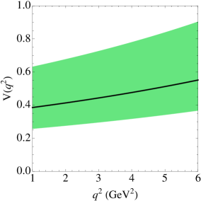
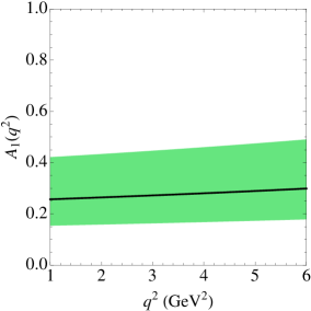
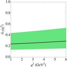
In principle, due to the large-recoil symmetry relations among the form factors that are valid up to corrections of order and , one is entitled to define also in terms of (see Eq. (24) of Ref. [40]). The resulting soft form factor is in very good agreement with the one obtained from Eq.(13).
The values of the soft form factors at zero are determined by
| (16) |
which corresponds to and . Notice that can be determined also through (see Eq. (13)) due to the large recoil relation . In order to correctly account for the correlation between the errors of and we determine using from KMPW. In Ref. [35] a slightly different normalization for is used, that is obtained from and not after including an correction.
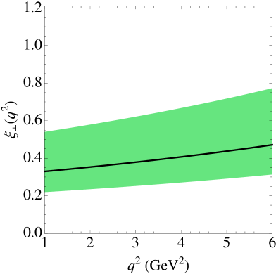
Once and are defined using Eq. (14), with , and the input values given in Table 2 (see Fig. 2), all form factors follow using [40]
| (17) |
where the first relation has no corrections at first order (). The second relation comes from the definition of the prescription, while the third one includes an correction explicitly inside the factor , where when (see [40] for the explicit definition of ).
One can compare the axial form factors defined from Eq. (17) with the values obtained from light-cone sum rules in the case of KPMW. We have checked explicitly that obtained from Eq. (17) exhibits a very good compatibility with the value computed by KMPW, which was expected as their results for and fulfilled the large recoil relations in Eq. (7) satisfactorily within errors. The same holds for with a similar small deviation. On the contrary the last relation of Eq. (17) exhibits a sizeable difference in the comparison between the obtained from KMPW (red-meshed region in Fig. 3) and the from Eq. (17) (blue-meshed region in Fig. 3), pointing to non-negligible corrections. Consequently, we have enlarged the error size of to cover both determinations, as shown in Fig. 3. Notice that the form factor only enters in the amplitude which is always suppressed by , so that this choice will have only a limited impact on our discussion.

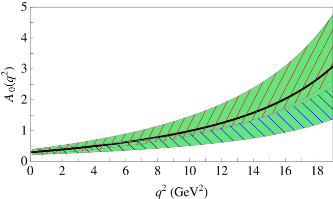
| Form factor | (GeV) | ||
|---|---|---|---|
In conclusion, in the large recoil region, once we determine and using Eq. (14) and the numerical inputs of Table 2, we obtain the form factors and from Eqs. (17). The form factor appearing in the amplitude is shown in Fig. (3). Finally, the tensor form factors (or ), required in the QCDF expression of amplitudes, are computed following Ref. [35]. The results are extrapolated up to 8.68 GeV2 to allow a complete comparison with experimental data. The resulting and are inserted in the QCDF-corrected form factors [35] required to compute the transversity amplitudes for , including all factorizable and non-factorizable corrections at one loop.
3.2 Low recoil
In the low-recoil region, the form factors cannot be determined in the same manner. The light-cone sum rule approach is valid at low-, and the results in KMPW are presented as valid only up to GeV2. However, following Refs. [24, 25] we will extrapolate them up to 19 GeV2 and check the consistency with the lattice QCD results which can be obtained at high- [41]. As for the large recoil region we will use KMPW form factors in order to remain conservative.

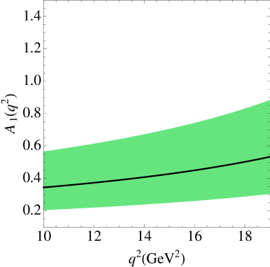
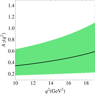
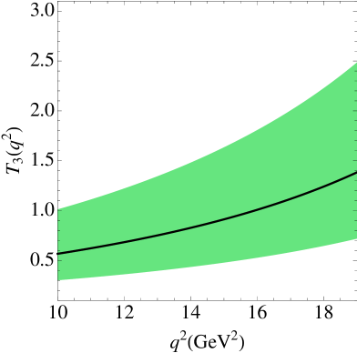
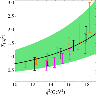
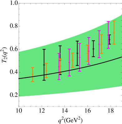
In this region where all degrees of freedom are soft, we expect the heavy-quark expansion to be a good approximation. Using this approach, in Ref. [21] a set of ratios were found that are expected to approach one in the exact symmetry limit, but away from this limit are broken by and corrections. This idea was reconsidered in Ref. [24], where three ratios were introduced:
| (18) |
In Ref. [24] the first two ratios were found to be near one, but the third one was found to be around 0.4.
This uncomfortable situation suggests one to reconsider these ratios. Indeed the first two of those ratios can be also found in Ref. [21] (see Eq. (A35) and Eq. (A36) in that reference), but the last ratio, corresponding to Eq. (A37), exhibits a more complicated structure:
| (19) |
We have checked that in the KMPW case the ratio is indeed in the correct ballpark. The discrepancy between the two versions of is rooted in the scaling laws of the form factors according to HQET power counting (see Eq. (A4) of Ref. [21]). According to these rules, the three terms in the denominator of are of different order in , so that and are equivalent according to this power counting. However the central values of the form factors extrapolated from light-cone sum rule results do not seem to obey the HQET power counting numerically, so that the three terms in the denominator of Eq. (19) are numerically competing and yield a poorly determined value for once uncertainties are taken into account.
In order to ensure the robustness of our results, given the problem with the definition of , we choose to proceed as follows. We determine and by exploiting the first two ratios () allowing for a 20% breaking, i.e., (with ). For all other form factors (including ) we use KMPW extrapolated in the high- region, as shown in Fig. 4. We then compare with available lattice data [41] to validate the tensor form factors thus obtained. As can be seen in Fig. 5, we find an excellent agreement between our determination of the tensor form factors using and lattice data. This also serves as a test of the validity of the extrapolation for and .
One may be worried that we drop one of the HQET relationships to use a value for that does not fulfill the expected HQET relation, especially to discuss clean observables that have been built based on the existence of these HQET relationships. The problem is actually less acute than it may seem at first sight. Indeed, occurs only in , multiplied by a factor that vanishes at the no-recoil endpoint (with a fairly small derivative). The other terms contributing to the longitudinal transversity amplitudes are suppressed in the large- limit where , but they are sizeable for the physical values of the mesons. Indeed, in the range of the low-recoil region, one finds the following relative contributions:
| (20) |
| (21) |
where is just a normalization and all form factors are numbers of order 1 in this kinematic region. Therefore, contrary to e.g., , the numerical impact of is very small for the low-recoil values of the observables. Since plays only a marginal role in the discussion, we will keep the discussion on the construction of clean observables at low recoil assuming for simplicity that the relationship for in Eq. (18) holds, but for numerical estimates, we will use the extrapolation of according to KMPW. On the long term, an accurate lattice estimate for would be the best way to settle this uneasy situation and check the validity of the ratio , exactly as for .
In summary, the main two differences in our treatment of form factors in this region with respect to Ref. [24] is that we use a more conservative approach to form factors and that we do not use all the relations between and , implied by the heavy quark symmetry, but only the two ratios () validated by a comparison to lattice data.
4 Definition of clean CP conserving and CP violating observables in -bins
Following Refs. [17, 23], we have to consider a further experimental effect: the various observables are obtained by fitting -binned angular distributions, so that the experimental results for the various observables must be compared to (functions of) the angular coefficients and integrated over the relevant kinematic range. Therefore we define the CP-averaged and CP-violating observables and , integrated in bins, as:
| (22) | ||||||
| (23) | ||||||
| (24) |
| (25) | ||||||
| (26) | ||||||
| (27) |
where the normalization is defined as
| (28) |
We also introduce the redundant111As was noted in Ref. [23] the symmetries of the distribution show that can be expressed in terms of all other observables (up to a sign, see appendix in Ref. [23]) and in this sense it is redundant. However, the binning procedure (or scalar contributions) will break this redundancy, recovered only in the limit of vanishing bin widths and in the absence of scalars. quantity defined in Ref. [23], and its CP-conjugated counterpart:
| (29) |
These definitions are general: they hold for and in the presence of scalar and tensor operators. In the limit of infinitesimal binning the definitions of coincide with the definitions in Ref. [17] except for a factor of in . This factor was introduced in Ref. [17] in the differential definition of precisely to cancel an explicit dependence in the numerator and make the observable insensitive to the lepton mass. However, in defining a binned observable (as noted in Ref. [26]) this cancellation takes place only approximately and there is no more compelling reason to remove this factor.
Using the arguments in Refs. [17] and [24], it is not difficult to check the status of these observables at low and large in relation with Table 1. All these observables are indeed built by considering a particular angular coefficient and normalizing it to cancel form factors in the appropriate region, as explained in Sec. 2. Besides these clean observables, we consider also quantities often discussed: the differential (CP-averaged) branching ratio , the CP asymmetry , the CP-averaged forward-backward asymmetry and longitudinal polarization fraction , and the corresponding CP asymmetries and . The definitions for the binned observables in terms of the integrated angular coefficients are:
| (30) | ||||||
| (31) | ||||||
| (32) |
where
| (33) |
and analogously for .
Some of these observables are related to others that have been defined in the literature. For example (see [17]) [14], , [18], [24, 25], as well as
| (34) |
where in terms of the angular coefficients, the observables are given by222We drop a factor of in with respect to Ref. [25]. The arguments are the same as the ones given above for . [25]
| (35) | |||||
| (36) |
The definitions for the integrated unprimed observables are given in App. A.
The CP asymmetry is related (but not equal) to the low-recoil observable [33], which is the CP-violating partner of . At low recoil (in the absence of scalar or tensor operators [25]) is also equal to the CP-violating partner of which is related (but not equal) to , defined in App. A. Analogously, the asymmetry is related at low recoil to [25] (CP-violating partner of ). At low recoil and in the absence of tensor operators this asymmetry is equal to the CP-violating partner of , related to (cf. Eq. (34)). Again this equivalence is not true at large recoil. Besides , we will consider this CP asymmetry related to in the full region, which we shall call . The exact definitions for and are given in App. A. Finally, the asymmetries and are related to of Ref. [33]. We recall that Table 1 provides a summary of the equivalence of the observables and their experimental and theoretical status.
In the following sections we will study these integrated observables in detail, giving predictions within the SM and studying their sensitivity to hadronic uncertainties and also to New Physics.
5 SM predictions for integrated observables
In this section we provide SM predictions for the set of integrated observables defined in Section 4. We focus on the binning most commonly used by experimental collaborations (see Refs. [3, 28, 42, 43, 44, 45]): [0.1,2], [2,4.3], [4.3,8.68] and [1,6] GeV2 at large recoil, [14.18,16] and [16,19] GeV2 at low recoil, and a bin between the two narrow resonances, [10.09,12.89] GeV2. Some of these bins contain regions outside the strict range of application of the corresponding theoretical frameworks. First, the region of very large recoil GeV2 contains contributions from light resonances which are not accounted for in QCDF. A thorough analysis of this region has been performed in Ref. [32], and some of its features are recalled in Section 8. However we will not include the effect of these light resonances in our results, as their impact is small on integrated quantities considered here. Second, the region GeV2 can be affected by non-negligible charm-loop effects (see Ref. [37]). Within the middle bin [10.09,12.89] GeV2, in between the and peaks, the charm-loop contribution leads to a destructive interference, leading to a suppression of the decay rate in this region. However, the predictions within this region should be considered as crude estimates [37]. In this paper, this region will be treated by interpolating central values and errors between the large and low recoil regions.
| -0.2632 | 1.0111 | -0.0055 | -0.0806 | 0.0004 | 0.0009 | -0.2923 | -0.1663 | 4.0749 | -4.3085 |
Our SM predictions are obtained in the usual way. The integrated observables are defined in Eqs. (22)-(32) in terms of the coefficients , which are simple functions of the transversity amplitudes (see for example Ref. [17]). The transversity amplitudes can be written in terms of Wilson coefficients and form factors following Refs. [19, 35, 24]. Concerning the Wilson coefficients and the treatment of uncertainties, we proceed as in Refs. [17, 23]. In particular, the SM Wilson coefficients are computed at the matching scale , and run down to the hadronic scale following Refs. [46, 47, 48, 49, 50] 333The slightly different values of and compared to the usual values encountered in the literature stems from the fact that we include higher-order electromagnetic corrections in the evaluation of these coefficients following the formulae gathered in Ref [46]. In particular, Table 5 in that reference shows that and are affected by subleading but not negligible corrections in , denoted and . This yields a shift compared to analyses not including higher-order electromagnetic corrections in the evaluation of their coefficients. (See also Ref. [51]). The evolution of couplings and quark masses proceeds analogously. All relevant input parameters used in the numerical analysis, including the values of the SM Wilson coefficients at the scale , are collected in Tables 3 and 4.
| [52] | |||
| [53] | [53] | ||
| [53] | [53] | ||
| [53] | |||
| [53] | [53] | ||
| [52] | [53] | ||
| [54] | [55] | ||
| [53] | [53] | ||
| [56] | [56] | ||
| [56] | [56] | ||
| [57] | [58] | ||
| GeV | [22] | [22] | |
| [22] | [22] | ||
| [22] | GeV | [53] |
Concerning uncertainties related to corrections, we proceed as follows. In the large recoil region we include a 10% multiplicative error in each amplitude, with an arbitrary strong phase, implemented as described in Refs. [16, 17]. In the low recoil region, we allow for a 20% correction to the ratios and , as described in Section 3.2, so that . We note that this correction is suppressed by a factor with respect to the dominant part of the amplitude [see Eqs. (4) and (5)]. In the SM , so the total correction is a few percent, as noticed in Ref. [33]. However, in some NP scenarios this suppression might not be so effective.
The results are collected in Tables 5 and 5, and in App. B, and they exhibit some expected behaviours. CP asymmetries are very small. and , related to and which involve suppressed helicity form factors in the low region [32] are null tests of the Standard Model for the first bins [14, 18]. In addition, and involve combinations of form factors which become equal in the low-recoil limit, and are thus very close to 1 and -1, respectively, for the last bins [24].
Table 5. Standard Model Predictions for the CP-averaged optimized basis.
| Bin (GeV2) | |||
|---|---|---|---|
| [ 1 , 2 ] | |||
| [ 0.1 , 2 ] | |||
| [ 2 , 4.3 ] | |||
| [ 4.3 , 8.68 ] | |||
| [ 10.09 , 12.89 ] | |||
| [ 14.18 , 16 ] | |||
| [ 16 , 19 ] | |||
| [ 1 , 6 ] | |||
| [ 1 , 2 ] | |||
| [ 0.1 , 2 ] | |||
| [ 2 , 4.3 ] | |||
| [ 4.3 , 8.68 ] | |||
| [ 10.09 , 12.89 ] | |||
| [ 14.18 , 16 ] | |||
| [ 16 , 19 ] | |||
| [ 1 , 6 ] | |||
| [ 1 , 2 ] | |||
| [ 0.1 , 2 ] | |||
| [ 2 , 4.3 ] | |||
| [ 4.3 , 8.68 ] | |||
| [ 10.09 , 12.89 ] | |||
| [ 14.18 , 16 ] | |||
| [ 16 , 19 ] | |||
| [ 1 , 6 ] |
Table 6. Standard Model Predictions for the CP-violating optimized basis.
| Bin (GeV2) | |||
|---|---|---|---|
| [ 1 , 2 ] | |||
| [ 0.1 , 2 ] | |||
| [ 2 , 4.3 ] | |||
| [ 4.3 , 8.68 ] | |||
| [ 10.09 , 12.89 ] | |||
| [ 14.18 , 16 ] | |||
| [ 16 , 19 ] | |||
| [ 1 , 6 ] | |||
| [ 1 , 2 ] | |||
| [ 0.1 , 2 ] | |||
| [ 2 , 4.3 ] | |||
| [ 4.3 , 8.68 ] | |||
| [ 10.09 , 12.89 ] | |||
| [ 14.18 , 16 ] | |||
| [ 16 , 19 ] | |||
| [ 1 , 6 ] | |||
| [ 1 , 2 ] | |||
| [ 0.1 , 2 ] | |||
| [ 2 , 4.3 ] | |||
| [ 4.3 , 8.68 ] | |||
| [ 10.09 , 12.89 ] | |||
| [ 14.18 , 16 ] | |||
| [ 16 , 19 ] | |||
| [ 1 , 6 ] |


6 New Physics opportunities
Our main motivation has consisted in finding an optimal basis for the analysis of data, with a balance between the theoretical control on hadronic pollution and the experimental accessibility. The importance of finding clean observables for NP searches has been emphasized in Ref. [23]. It has been shown that, while a NP contribution to an angular coefficient can be substantial, a non-clean observable sensitive to the coefficient (such as itself, or ) might not be able to detect such NP because of large theoretical uncertainties, even if the SM prediction for this observable is accurate. On the contrary, the corresponding clean observable might show a clear distinction between the SM and the NP scenario even once theoretical uncertainties are included.
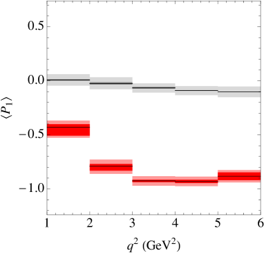
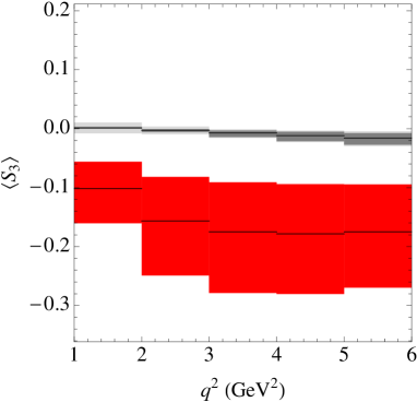
This feature has been exemplified in Ref [23] studying the observables and both in the SM and within a NP benchmark point compatible with other constraints from rare decays. In Fig. 8 we update this discussion by showing binned predictions at large recoil for and in the SM and in the NP scenario given by (where ). Clearly, is much more sensitive to New Physics than , due to its reduced hadronic uncertainties.
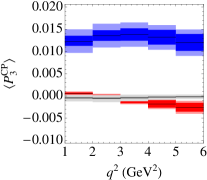
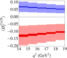
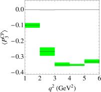
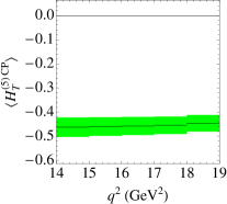
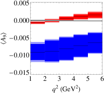
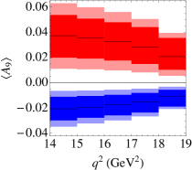
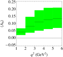
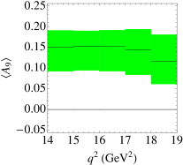
A similar conclusion can be reached in the case of CP-violating observables. For illustration, we consider the case of CP-violating observables related to the angular coefficient . The observable is not a clean observable, while is the corresponding clean observable in the large recoil region. At low recoil, the clean observable is also considered. In Fig. 9 we show binned predictions for , and in the SM and in three NP scenarios: two scenarios with complex left-handed currents given by and , and a scenario with a complex contribution to : . These scenarios are consistent with all current constraints [59]. The SM prediction is very close to zero for all these observables. But a departure from the SM point has a dramatic effect in the hadronic uncertainties in the prediction of . On the other hand, the clean observables and , designed for low and high- regions respectively, are much more robust.
These examples show how (at large recoil) and (at low recoil) present unique opportunities to discover or constrain New Physics, and should be given priority over the non-clean observable . More generally, they illustrate the interest of choosing clean observables to distinguish between the SM case and NP scenarios from a binned angular analysis of the decay.
7 Impact of the S-wave pollution
Another source of uncertainties come for the S-wave contribution on the angular distribution , which will correspond to a pollution of the angular observables extracted under the assumption that the process is only mediated through P-wave decaying into .
In Ref. [29] the S-wave pollution to the decay coming from the companion decay was computed. The model used there assumed that both and waves were correctly described by -dependent or form factors, multiplied by a Breit-Wigner function depending on the invariant mass (possibly distorted by non-resonant effects such as the elusive or resonance [60])444This model has the advantage of simplicity, as it factorises the dependence of the amplitudes on the dilepton and the dihadron masses into two different pieces. However, it should be understood as a rough description of off-shell effects, as it hinges on the assumptions that the or form factors are not significantly altered once the light strange meson is not on shell any more, and that the coupling is essentially independent of the dihadron mass from threshold up to around 2 GeV.. It was then claimed that transverse asymmetries, obtained from uni-angular distributions, suffer unavoidably the S-wave contamination. Soon after and in the same framework, it was shown in Ref. [26] that using folded distributions instead of uni-angular distributions it should be possible to extract those asymmetries free from this pollution. Indeed, due to the distinct angular dependence of the S-wave terms one can disentangle the interesting signal of the P-wave from the S-wave polluting terms. However an additional problem arises due to the normalization used for the distribution, that we will discuss in the following.
The angular distribution that describes the four-body decay including the S-wave pollution from the companion decay is [29, 30]
| (37) | |||||
where new angular coefficients arise (including a Breit-Wigner function in their definition)
| (38) | |||||
as well as a factor included to take into account the width of the resonance:
| (39) |
One can consider for the normalization of the angular distribution not the P-wave component alone () but the sum of S and P wave amplitudes (including both the and components) defined by
| (40) |
where we denote () with the distribution of the . Their expression in terms of the angular coefficients are (see Refs. [29, 26] for detailed definitions of the new coefficients )
| (41) |
and the longitudinal polarization fraction associated to the distribution is
| (42) |
As pointed out in Ref. [26] (see Eq. (23)), the use of the normalization for the angular distribution induces a polluting factor (called in Ref. [26] or equivalently here) that multiplies the P-wave component distribution. For simplicity, in order to obtain the bounds on the polluting terms entering we will work with the distribution in the massless lepton limit (the distribution in the massive case is discussed in Ref. [26])
| (43) | |||||
The coefficients of the polluting term can be parametrized as
| (44) | |||||
where we have used the equalities in the massless limit and .
We will now estimate the size of the S-wave polluting terms () normalized to . Identifying the coefficients in Eq.(44) with Eq.(38) we find:
| (45) |
with . From the explicit expressions of the (see Ref. [26] for definitions) one finds for 555The amplitudes used here are proportional to those introduced in Ref. [29]: and . Notice that here , where cancels between numerator and denominator.
| (46) |
with a factor included to take into account the scalar component including the resonance. The corresponding lineshape is denoted , even though it is likely not to be a simple Breit-Wigner shape, due to the possibility of a non-trivial scalar continuum. The contribution from the -wave is expected to be small compared to the -wave one.
The other terms in Eq.(44) comes from the - and -wave interference and are
| (47) |
A bound on these ratios is obtained once we define the interference integral
| (48) |
and use the bound from the Cauchy-Schwartz inequality
| (49) |
| Coefficient | Large recoil Range | Low recoil Range | Large Recoil Finite Range | Low Recoil Finite Range |
|---|---|---|---|---|
The definitions of and yield the following bound:
| (50) |
where the factor arises due to the fact that is defined with respect to rather than . Using the definition of in terms of one finds for the other terms in Eq.(44) the following bounds
| (51) |
In order to assign a numerical value to these bounds we have to evaluate the integrals , and that enter the factor . Here we can consider two options: a first option that we call “infinite range” where we take the integrals in the whole range. In this case, we get , and . And a second option where we consider a “finite range” for the integrals around GeV (corresponding to the constraints put on the invariant dihadron mass for the experimental analysis), we use the parametrization given in [18], and we vary the parameters of the Breit-Wigner ( and inside range) to obtain . Similarly for the other integrals one gets in this case and . And the corresponding factor is now inside the range .
We can provide two illustrative examples for the large- and low-recoil regions. We take in the large-recoil region the following values [61] (assuming that the scalar contribution is similar to that in the decay ), and , and for the low recoil region, the same value of , and , where the values for and are the average of the central values of the SM predictions in the last two bins. For the factor we take the maximal possible values. The corresponding bounds are gathered in Table 7. These estimates can be more precise once we have a direct measurement of .
8 Comparison with other works
In addition to general global fits to radiative -decays [23, 59, 62] (see also Refs. [63, 64, 65, 66, 67, 68]), there has been a growing literature aiming at determining the best set of observables with a reduced sensitivity to hadronic inputs, and the ability of these observables to find New Physics.
Compared to Ref. [22], we obtain a fair agreement with the predictions of the and within errors, even if we take a different approach for the treatment of form factors and different input values for them. On top of this, there is also some difference on the Wilson coefficient values for dileptonic operators where we included extra electromagnetic corrections. In some cases like or the tiny asymmetry the agreement with the central value is perfect. But as these observables are not protected from hadronic uncertainties in general, there are cases where the SM value is tiny (e.g., for ) and basically driven by NLO contributions, where the result is more sensitive to the use of full form factors or of specific relationships derived from an effective theory approach, and to the input values chosen.
The high- region has been the focus of a series of papers [24, 33, 25], relying on relationships between form factors from the heavy-quark expansion derived in Ref. [21] (as discussed in Section 3). In Refs. [24, 25], a set of 5 clean (CP-averaged) observables called was introduced, which is equivalent to the set introduced here for clean observables at high-. The corresponding CP-violating observables were also discussed, as well as the case of transitions (with only 3 angular observables avalaible), and their potential for New Physics. We confirm that CP-averaged observables (e.g., ) have a small sensitivity to hadronic uncertainties, but we stress that this needs not be the case for CP-violating observables in the presence of New Physics. We agree with the numerical results for the SM predictions of , but we quote larger uncertainties in particular for the branching ratio. This is due most probably to a different choice of form factors (Ref. [38] (BZ) versus KMPW [37]). As discussed in Ref. [24] and discussed again in Section 3, there are some difficulties to accomodate the extrapolation of BZ form factors at high with the HQET relationships exploited to compute the angular coefficients. We have discussed the comparison with available lattice data and our choice of using KMPW together with HQET relationships until accurate lattice data are available for the low-recoil region.
The low- has been discussed in Ref. [32] recently, with an interpretation of angular observables in terms of helicity form factors [39]. The pattern of suppression of some form factors with respect to others, indicated by QCD factorisation/SCET analyses, was shown to hold even after the inclusion of radiative and power corrections as well as non-factorisable effects and to yield a strong suppression of the angular coefficients and . For the phenomenological analyses, several inputs for the form factors were considered, not only (rescaled) BZ and KMPW, but also QCD sum rules and truncated Dyson-Schwinger equations. The comparison of the various models confirmed corrections of a few percent to the QCD factorisation/SCET relationships, in the line of the estimates used in this paper. But if some of the angular coefficients are dominated by form factor uncertainties, sizeable contributions may also arise from charm-loop contributions. Compared to our own analysis, we have allowed for a larger range of uncertainties concerning form factors, but no charm-loop contributions. This explains the agreement concerning the central values for the low- observables, but significantly larger errors in Ref. [32] (especially for and ). The very low- region (below 1 GeV2) was also analysed, using a phenomenological model to account for light resonances. The effect of the latter was shown to be very small once binning effects were including, and has not been considered in our own analysis.
The issue of long-distance charm loop effects was also considered in Ref. [37]. This paper was aimed at calculating one particular effect, the soft-gluon emission from the charm loop, which is only one of the several nonlocal hadronic effects for caused by four-quark, quark-penguin and operators. The modification induced to was encoded in a shift where only the factorizable charm loop and nonfactorizable soft gluon are taken into account, up to 20% in the low- region (below 4 GeV2). It is interesting to notice that this particular effect is difficult to assess and can be large, casting some doubts on the possibility to exploit the bins between and for comparison with experiment. We have not included the results of Refs. [37, 32] waiting for a more comprehensive theory of charm-loop effects before including them in our analysis.
9 Conclusions
Measurements on the angular distribution of the decay are being performed intensively at flavour facilities. In the near future, these measurements will either reveal hints of NP in flavour physics, or set the strongest constraints so far on radiative and semileptonic operators. However, in order for these measurements to be effective, the focus has to be put on theoretically “clean” observables.
In this paper we have studied and collected all relevant clean angular observables in both kinematic regions of interest (large and low recoils), giving a unified and comprehensive description of both regions, and a thorough reassessment of the form factor input. We have also considered a full set of CP-violating observables, . We reviewed the various observables proposed in Table 1, and we can identify an optimal basis containing a maximal number of clean observables that constitutes a compromise between a clean theoretical prediction and a simple experimental extraction. All SM predictions can be found in Tables 5-5 in Sec. 5 and Tables B-B in App. B.
The relevance in focusing on clean observables can be seen more clearly by studying the NP sensitivity of different observables probing in principle the same angular coefficient, but with a normalisation enhancing or suppressing the sensitivity to form factors. By considering different NP scenarios (compatible with current bounds) we find that is much more sensitive than to NP effects due to it reduced hadronic uncertainties. The same is found for the CP asymmetries (at large recoil) and (at low recoil), which are much finer probes of NP than .
An important systematic effect that has to be fully understood is the S-wave component due to events, which is not negligible even at . Disentangling the S- and P-wave contributions requires a more complete angular analysis, which if not performed leads to intrinsic systematics in the extraction of the angular observables. We have determined bounds on the size of the interference terms in the angular distribution, which constitute an upper bound on these systematic uncertainties.
By providing an appropriate basis with a limited sensitivity to hadronic contributions and thus a better potential to identify New Physics contributions, and by giving SM predictions for these observables, we hope that the results and predictions presented in this paper will help the discussion of the next series of results on .
Acknowledgments
It is a pleasure to thank Nicola Serra and Thorsten Feldmann for discussions and comments. J.M. enjoys financial support from FPA2011-25948, SGR2009-00894. J.V. is supported in part by ICREA-Academia funds and FPA2011-25948.
Appendix A Definitions of additional observables
The integrated unprimed observables are given by
| (52) | ||||||
| (53) | ||||||
| (54) | ||||||
| (55) |
where and are defined as
| (56) | |||
| (57) |
The CP-violating observables are given by
| (58) | |||||
| (59) |
Appendix B Compendium of SM results
In this Appendix we collect the SM predictions for the observables discussed in the paper in addition to Tables 5 and 5, where the observables in the optimized CP-averaged and CP-violating bases are collected. All these results are also presented graphically in Figures 6-12. The binning is chosen to match the current experimental results. Predictions within different bins can be obtained as explained in the text, and are also available upon request.
The second series of errors quoted correspond to corrections, whereas the first series stem from all uncertainties in the inputs, and in particular in form factors. They have been obtained following the method presented in Refs. [15, 16, 17], as outlined in Section 5.
Table 8. Standard Model Predictions for CP-averaged observables.
| Bin (GeV2) | |||
|---|---|---|---|
| [ 1 , 2 ] | |||
| [ 0.1 , 2 ] | |||
| [ 2 , 4.3 ] | |||
| [ 4.3 , 8.68 ] | |||
| [ 10.09 , 12.89 ] | |||
| [ 14.18 , 16 ] | |||
| [ 16 , 19 ] | |||
| [ 1 , 6 ] | |||
| [ 1 , 2 ] | |||
| [ 0.1 , 2 ] | |||
| [ 2 , 4.3 ] | |||
| [ 4.3 , 8.68 ] | |||
| [ 10.09 , 12.89 ] | |||
| [ 14.18 , 16 ] | |||
| [ 16 , 19 ] | |||
| [ 1 , 6 ] | |||
| [ 1 , 2 ] | |||
| [ 0.1 , 2 ] | |||
| [ 2 , 4.3 ] | |||
| [ 4.3 , 8.68 ] | |||
| [ 10.09 , 12.89 ] | |||
| [ 14.18 , 16 ] | |||
| [ 16 , 19 ] | |||
| [ 1 , 6 ] |
Table 9. Standard Model Predictions for CP-violating observables.
| Bin (GeV2) | |||
|---|---|---|---|
| [ 1 , 2 ] | |||
| [ 0.1 , 2 ] | |||
| [ 2 , 4.3 ] | |||
| [ 4.3 , 8.68 ] | |||
| [ 10.09 , 12.89 ] | |||
| [ 14.18 , 16 ] | |||
| [ 16 , 19 ] | |||
| [ 1 , 6 ] | |||
| [ 1 , 2 ] | |||
| [ 0.1 , 2 ] | |||
| [ 2 , 4.3 ] | |||
| [ 4.3 , 8.68 ] | |||
| [ 10.09 , 12.89 ] | |||
| [ 14.18 , 16 ] | |||
| [ 16 , 19 ] | |||
| [ 1 , 6 ] | |||
| [ 1 , 2 ] | |||
| [ 0.1 , 2 ] | |||
| [ 2 , 4.3 ] | |||
| [ 4.3 , 8.68 ] | |||
| [ 10.09 , 12.89 ] | |||
| [ 14.18 , 16 ] | |||
| [ 16 , 19 ] | |||
| [ 1 , 6 ] |
Table 10. Standard Model Predictions for CP-averaged observables.
| Bin (GeV2) | |||
|---|---|---|---|
| [ 1 , 2 ] | |||
| [ 0.1 , 2 ] | |||
| [ 2 , 4.3 ] | |||
| [ 4.3 , 8.68 ] | |||
| [ 10.09 , 12.89 ] | |||
| [ 14.18 , 16 ] | |||
| [ 16 , 19 ] | |||
| [ 1 , 6 ] | |||
| [ 1 , 2 ] | |||
| [ 0.1 , 2 ] | |||
| [ 2 , 4.3 ] | |||
| [ 4.3 , 8.68 ] | |||
| [ 10.09 , 12.89 ] | |||
| [ 14.18 , 16 ] | |||
| [ 16 , 19 ] | |||
| [ 1 , 6 ] | |||
| [ 1 , 2 ] | |||
| [ 0.1 , 2 ] | |||
| [ 2 , 4.3 ] | |||
| [ 4.3 , 8.68 ] | |||
| [ 10.09 , 12.89 ] | |||
| [ 14.18 , 16 ] | |||
| [ 16 , 19 ] | |||
| [ 1 , 6 ] |
Table 11. Standard Model Predictions for CP-violating observables.
| Bin (GeV2) | |||
|---|---|---|---|
| [ 1 , 2 ] | |||
| [ 0.1 , 2 ] | |||
| [ 2 , 4.3 ] | |||
| [ 4.3 , 8.68 ] | |||
| [ 10.09 , 12.89 ] | |||
| [ 14.18 , 16 ] | |||
| [ 16 , 19 ] | |||
| [ 1 , 6 ] | |||
| [ 1 , 2 ] | |||
| [ 0.1 , 2 ] | |||
| [ 2 , 4.3 ] | |||
| [ 4.3 , 8.68 ] | |||
| [ 10.09 , 12.89 ] | |||
| [ 14.18 , 16 ] | |||
| [ 16 , 19 ] | |||
| [ 1 , 6 ] | |||
| [ 1 , 2 ] | |||
| [ 0.1 , 2 ] | |||
| [ 2 , 4.3 ] | |||
| [ 4.3 , 8.68 ] | |||
| [ 10.09 , 12.89 ] | |||
| [ 14.18 , 16 ] | |||
| [ 16 , 19 ] | |||
| [ 1 , 6 ] |
Table 12. Standard Model Predictions for CP-averaged observables.
| Bin (GeV2) | |||
|---|---|---|---|
| [ 1 , 2 ] | |||
| [ 0.1 , 2 ] | |||
| [ 2 , 4.3 ] | |||
| [ 4.3 , 8.68 ] | |||
| [ 10.09 , 12.89 ] | |||
| [ 14.18 , 16 ] | |||
| [ 16 , 19 ] | |||
| [ 1 , 6 ] |


References
- [1] Belle Collaboration, “Measurement of with a Hadronic Tagging Method Using the Full Data Sample of Belle,” arXiv:1208.4678 [hep-ex].
- [2] LHCb Collaboration, “Measurement of the flavour-specific CP violating asymmetry in decays,” LHCb-CONF-2012-022.
- [3] LHCb Collaboration, “Measurement of the isospin asymmetry in decays,” JHEP 1207, 133 (2012) [arXiv:1205.3422 [hep-ex]].
- [4] T. Feldmann and J. Matias, “Forward backward and isospin asymmetry for decay in the standard model and in supersymmetry,” JHEP 0301, 074 (2003) [hep-ph/0212158].
- [5] CDF Collaboration, “Search for and Decays with CDF II,” Phys. Rev. Lett. 107, 239903 (2011) [Phys. Rev. Lett. 107, 191801 (2011)] [arXiv:1107.2304 [hep-ex]].
- [6] CMS Collaboration, S. Chatrchyan et al., “Search for and decays,” JHEP 1204, 033 (2012) [arXiv:1203.3976 [hep-ex]].
- [7] ATLAS Collaboration, G. Aad et al., “Search for the decay with the ATLAS detector,” Phys. Lett. B 713, 387 (2012) [arXiv:1204.0735 [hep-ex]].
- [8] LHCb Collaboration, “First evidence for the decay ,” Phys. Rev. Lett. 110, 021801 (2013) [arXiv:1211.2674 [Unknown]].
- [9] A. Buras, J. Girrbach, D. Guadagnoli, G. Isidori, “On the Standard Model prediction for ,” Eur. Phys. J. C 72, 2172 (2012) [arXiv:1208.0934 [hep-ph]].
- [10] LHCb Collaboration, “First observation of the decay ,” Phys. Lett. B 709, 50 (2012) [arXiv:1111.4183 [hep-ex]].
- [11] S. Descotes-Genon, J. Matias and J. Virto, “An analysis of mixing angles in presence of New Physics and an update of ,” Phys. Rev. D 85, 034010 (2012) [arXiv:1111.4882 [hep-ph]].
- [12] Babar Collaboration “Evidence for an excess of decays,” Phys. Rev. Lett. 109, 101802 (2012) [arXiv:1205.5442 [hep-ex]].
- [13] S. Fajfer, J. F. Kamenik and I. Nisandzic, “On the Sensitivity to New Physics,” Phys. Rev. D 85, 094025 (2012) [arXiv:1203.2654 [hep-ph]].
- [14] F. Kruger and J. Matias, “Probing new physics via the transverse amplitudes of at large recoil,” Phys. Rev. D 71, 094009 (2005) [hep-ph/0502060].
- [15] U. Egede, T. Hurth, J. Matias, M. Ramon and W. Reece, “New observables in the decay mode ,” JHEP 0811, 032 (2008) [arXiv:0807.2589 [hep-ph]].
- [16] U. Egede, T. Hurth, J. Matias, M. Ramon and W. Reece, “New physics reach of the decay mode ,” JHEP 1010, 056 (2010) [arXiv:1005.0571 [hep-ph]].
- [17] J. Matias, F. Mescia, M. Ramon and J. Virto, “Complete Anatomy of and its angular distribution,” JHEP 1204, 104 (2012) [arXiv:1202.4266 [hep-ph]].
- [18] D. Becirevic, E. Schneider, “On transverse asymmetries in ,” Nucl. Phys. B 854, 321 (2012) [arXiv:1106.3283 [hep-ph]].
- [19] M. Beneke, T. Feldmann and D. Seidel, “Systematic approach to exclusive , decays,” Nucl. Phys. B 612, 25 (2001) [hep-ph/0106067].
- [20] J. Charles, A. Le Yaouanc, L. Oliver, O. Pene and J. C. Raynal, “Heavy to light form-factors in the heavy mass to large energy limit of QCD,” Phys. Rev. D 60, 014001 (1999) [hep-ph/9812358].
- [21] B. Grinstein and D. Pirjol, “Exclusive rare decays at low recoil: Controlling the long-distance effects,” Phys. Rev. D 70, 114005 (2004) [hep-ph/0404250].
- [22] W. Altmannshofer, P. Ball, A. Bharucha, A. J. Buras, D. M. Straub and M. Wick, “Symmetries and Asymmetries of Decays in the Standard Model and Beyond,” JHEP 0901, 019 (2009) [arXiv:0811.1214 [hep-ph]].
- [23] S. Descotes-Genon, J. Matias, M. Ramon and J. Virto, “Implications from clean observables for the binned analysis of at large recoil,” JHEP 1301, 048 (2013) [arXiv:1207.2753 [hep-ph]].
- [24] C. Bobeth, G. Hiller and D. van Dyk, “The Benefits of Decays at Low Recoil,” JHEP 1007, 098 (2010) [arXiv:1006.5013 [hep-ph]].
- [25] C. Bobeth, G. Hiller and D. van Dyk, “General Analysis of Decays at Low Recoil,” arXiv:1212.2321 [hep-ph].
- [26] J. Matias, “On the S-wave pollution of observables,” Phys. Rev. D 86, 094024 (2012) [arXiv:1209.1525 [hep-ph]].
- [27] C. Bobeth, G. Hiller, and G. Piranishvili, “CP Asymmetries in bar and Untagged , Decays at NLO,” JHEP 0807, 106 (2008) [arXiv:0805.2525 [hep-ph]].
- [28] LHCb Collaboration, “Differential branching fraction and angular analysis of the decay”. Phys. Rev. Lett. 108, 181806 (2012), [LHCb-CONF-2012-008 and arXiv:1112.3515 [hep-ex]].
- [29] D. Becirevic and A. Tayduganov, “Impact of on the New Physics search in decay,” Nucl. Phys. B 868, 368 (2013) [arXiv:1207.4004 [hep-ph]].
- [30] C. -D. Lu, W. Wang and , “Analysis of in the higher kaon resonance region,” Phys. Rev. D 85, 034014 (2012) [arXiv:1111.1513 [hep-ph]].
- [31] T. Blake, U. Egede, A. Shires and , “The effect of S-wave interference on the angular observables,” JHEP 1303, 027 (2013) [arXiv:1210.5279 [hep-ph]].
- [32] S. Jäger and J. M. Camalich, “On at small dilepton invariant mass, power corrections, and new physics,” arXiv:1212.2263 [hep-ph].
- [33] C. Bobeth, G. Hiller, D. van Dyk, “More Benefits of Semileptonic Rare B Decays at Low Recoil: CP Violation,” JHEP 1107, 067 (2011) [arXiv:1105.0376 [hep-ph]].
- [34] C. Hambrock and G. Hiller, “Extracting Form Factors from Data,” Phys. Rev. Lett. 109, 091802 (2012) [arXiv:1204.4444 [hep-ph]].
- [35] M. Beneke, T. Feldmann and D. Seidel, “Exclusive radiative and electroweak and penguin decays at NLO,” Eur. Phys. J. C 41, 173 (2005) [hep-ph/0412400].
- [36] C. Bourrely, I. Caprini and L. Lellouch, “Model-independent description of decays and a determination of ,” Phys. Rev. D 79, 013008 (2009) [Erratum-ibid. D 82, 099902 (2010)] [arXiv:0807.2722 [hep-ph]].
- [37] A. Khodjamirian, T. Mannel, A. A. Pivovarov, Y. -M. Wang, “Charm-loop effect in and ,” JHEP 1009, 089 (2010) [arXiv:1006.4945 [hep-ph]].
- [38] P. Ball and R. Zwicky, “ decay form-factors from light-cone sum rules revisited,” Phys. Rev. D 71, 014029 (2005) [hep-ph/0412079].
- [39] A. Bharucha, T. Feldmann and M. Wick, “Theoretical and Phenomenological Constraints on Form Factors for Radiative and Semi-Leptonic B-Meson Decays,” JHEP 1009, 090 (2010) [arXiv:1004.3249 [hep-ph]].
- [40] M. Beneke and T. Feldmann, “Symmetry breaking corrections to heavy to light B meson form-factors at large recoil,” Nucl. Phys. B 592, 3 (2001) [hep-ph/0008255]. S. Descotes-Genon and A. Le Yaouanc, “Parametrisations of the form factor and the determination of ,” J. Phys. G 35 (2008) 115005 [arXiv:0804.0203 [hep-ph]].
- [41] D. Becirevic, V. Lubicz and F. Mescia, “An Estimate of the form factor,” Nucl. Phys. B 769, 31 (2007) [hep-ph/0611295].
- [42] Belle Collaboration, “Measurement of the Differential Branching Fraction and Forward-Backward Asymmetry for ,” Phys. Rev. Lett. 103, 171801 (2009) [arXiv:0904.0770 [hep-ex]].
- [43] CDF Collaboration, “Measurements of the Angular Distributions in the Decays at CDF,” Phys. Rev. Lett. 108, 081807 (2012) [arXiv:1108.0695 [hep-ex]].
- [44] BaBar Collaboration, “Measurement of Branching Fractions and Rate Asymmetries in the Rare Decays ,” [arXiv:1204.3933 [hep-ex]].
- [45] N. Serra [for the LHCb Collaboration], “Search for new physics in and ,” arXiv:1208.3987 [hep-ex].
- [46] T. Huber, E. Lunghi, M. Misiak and D. Wyler, “Electromagnetic logarithms in ,” Nucl. Phys. B 740, 105 (2006) [hep-ph/0512066].
- [47] P. Gambino, M. Gorbahn and U. Haisch, “Anomalous dimension matrix for radiative and rare semileptonic decays up to three loops,” Nucl. Phys. B 673, 238 (2003) [hep-ph/0306079].
- [48] M. Gorbahn and U. Haisch, “Effective Hamiltonian for non-leptonic decays at NNLO in QCD,” Nucl. Phys. B 713, 291 (2005) [hep-ph/0411071].
- [49] C. Bobeth, P. Gambino, M. Gorbahn and U. Haisch, “Complete NNLO QCD analysis of and higher order electroweak effects,” JHEP 0404, 071 (2004) [hep-ph/0312090].
- [50] M. Misiak and M. Steinhauser, “NNLO QCD corrections to the matrix elements using interpolation in ,” Nucl. Phys. B 764, 62 (2007) [hep-ph/0609241].
- [51] T. Huber, T. Hurth, E. Lunghi and , “Logarithmically Enhanced Corrections to the Decay Rate and Forward Backward Asymmetry in ,” Nucl. Phys. B 802, 40 (2008) [arXiv:0712.3009 [hep-ph]].
- [52] M. Misiak et al., “Estimate of at ,” Phys. Rev. Lett. 98, 022002 (2007) [hep-ph/0609232].
- [53] J. Beringer et al. (Particle Data Group), “Review of particle physics,” J. Phys. D86, 010001 (2012).
- [54] J. Alcaraz [ALEPH and CDF and D0 and DELPHI and L3 and OPAL and SLD Collaboration], “Precision Electroweak Measurements and Constraints on the Standard Model,” arXiv:0911.2604 [hep-ex].
- [55] C. W. Bauer, Z. Ligeti, M. Luke, A. V. Manohar and M. Trott, “Global analysis of inclusive B decays,” Phys. Rev. D 70, 094017 (2004) [hep-ph/0408002].
- [56] J. Charles et al. [CKMfitter Group Collaboration], “CP violation and the CKM matrix: Assessing the impact of the asymmetric factories,” Eur. Phys. J. C 41, 1 (2005) [hep-ph/0406184], and online update on http://ckmfitter.in2p3.fr/
- [57] A. L. Kagan and M. Neubert, “Isospin breaking in decays,” Phys. Lett. B 539, 227 (2002) [hep-ph/0110078].
- [58] C. Davies, “Standard Model Heavy Flavor physics on the Lattice,” PoS LATTICE 2011, 019 (2011) [arXiv:1203.3862 [hep-lat]].
- [59] W. Altmannshofer, P. Paradisi, D. Straub, “Model-Independent Constraints on New Physics in Transitions,” JHEP 1204, 008 (2012) [arXiv:1111.1257 [hep-ph]].
- [60] S. Descotes-Genon and B. Moussallam, “The scalar resonance from Roy-Steiner representations of scattering,” Eur. Phys. J. C 48 (2006) 553 [hep-ph/0607133].
- [61] B. Aubert et al. [BABAR Collaboration], “Ambiguity-free measurement of : Time-integrated and time-dependent angular analyses of ,” Phys. Rev. D 71 (2005) 032005 [hep-ex/0411016].
- [62] F. Beaujean, C. Bobeth, D. van Dyk and C. Wacker, “Bayesian Fit of Exclusive Decays: The Standard Model Operator Basis,” JHEP 1208, 030 (2012), arXiv:1205.1838 [hep-ph].
- [63] C. Bobeth, G. Hiller, D. van Dyk and C. Wacker, “The Decay at Low Hadronic Recoil and Model-Independent Constraints,” JHEP 1201, 107 (2012) [arXiv:1111.2558 [hep-ph]].
- [64] S. Descotes-Genon, D. Ghosh, J. Matias and M. Ramon, “Exploring New Physics in the plane,” JHEP 1106, 099 (2011) [arXiv:1104.3342 [hep-ph]]. S. Descotes-Genon, D. Ghosh, J. Matias and M. Ramon, “Exploring New Physics in ,” PoS EPS -HEP2011 (2011) 170 [arXiv:1202.2172 [hep-ph]].
- [65] D. Becirevic, E. Kou, A. L. Yaouanc and A. Tayduganov, “Future prospects for the determination of the Wilson coefficient ,” JHEP 1208, 090 (2012) [arXiv:1206.1502 [hep-ph]].
- [66] T. Hurth and F. Mahmoudi, “The Minimal Flavour Violation benchmark in view of the latest LHCb data,” Nucl. Phys. B 865, 461 (2012) [arXiv:1207.0688 [hep-ph]].
-
[67]
S. Descotes-Genon, J. Matias and J. Virto,
“New Physics constraints from optimized observables in at large recoil,”
AIP Conf. Proc. 1492, 103 (2012)
[arXiv:1209.0262 [hep-ph]].
S. Descotes-Genon, T. Hurth, J. Matias and J. Virto, “: The New Frontier of New Physics searches in Flavor,” arXiv:1305.4808 [hep-ph]. - [68] A. K. Alok, A. Datta, A. Dighe, M. Duraisamy, D. Ghosh and D. London, “New Physics in : CP-Conserving Observables,” JHEP 1111, 121 (2011) [arXiv:1008.2367 [hep-ph]]. A. K. Alok, A. Datta, A. Dighe, M. Duraisamy, D. Ghosh and D. London, “New Physics in : CP-Violating Observables,” JHEP 1111, 122 (2011) [arXiv:1103.5344 [hep-ph]].