Full-Wave Iterative Image Reconstruction in Photoacoustic Tomography with Acoustically Inhomogeneous Media

Abstract

Existing approaches to image reconstruction in photoacoustic computed tomography (PACT) with acoustically heterogeneous media are limited to weakly varying media, are computationally burdensome, and/or cannot effectively mitigate the effects of measurement data incompleteness and noise. In this work, we develop and investigate a discrete imaging model for PACT that is based on the exact photoacoustic (PA) wave equation and facilitates the circumvention of these limitations. A key contribution of the work is the establishment of a procedure to implement a matched forward and backprojection operator pair associated with the discrete imaging model, which permits application of a wide-range of modern image reconstruction algorithms that can mitigate the effects of data incompleteness and noise. The forward and backprojection operators are based on the k-space pseudospectral method for computing numerical solutions to the PA wave equation in the time domain. The developed reconstruction methodology is investigated by use of both computer-simulated and experimental PACT measurement data.

I Introduction

Photoacoustic computed tomography (PACT), also known as optoacoustic or thermoacoustic tomography, is a rapidly emerging hybrid imaging modality that combines optical image contrast with ultrasound detection. [1, 2, 3, 4] In PACT, the to-be-imaged object is illuminated with a pulsed optical wavefield. Under conditions of thermal confinement [5, 2], the absorption of the optical energy results in the generation of acoustic wavefields via the thermoacoustic effect. These wavefields propagate out of the object and are measured by use of wide-band ultrasonic transducers. From these measurements, a tomographic reconstruction algorithm is employed to obtain an image that depicts the spatially variant absorbed optical energy density distribution within the object, which will be denoted by the function $A(\mathbf{r})$. Because the optical absorption properties of tissue are highly related to its hemoglobin concentration and molecular constitution, PACT holds great potential for a wide-range of anatomical, functional, and molecular imaging tasks in preclinical and clinical medicine [3, 6, 7, 8, 9].

The majority of currently available PACT reconstruction algorithms are based on idealized imaging models that assume a lossless and acoustically homogeneous medium. However, in many applications of PACT these assumptions are violated and the induced photoacoustic (PA) wavefields are scattered and absorbed as they propagate to the receiving transducers. In small animal imaging applications of PACT, for example, the presence of bone and/or gas pockets can strongly perturb the photoacoustic wavefield. Another example is transcranial PACT brain imaging of primates [10], in which the PA wavefields can be strongly aberrated and attenuated [11, 12, 13] by the skull. In these and other biomedical applications of PACT, the reconstructed images can contain significant distortions and artifacts if the inhomogeneous acoustic properties of the object are not accounted for in the reconstruction algorithm.

Several image reconstruction methods have been proposed to compensate for weak variations in a medium’s speed-of-sound (SOS) distribution [14, 15, 16]. These methods are based on geometrical acoustic approximations to the PA wave equation, which stipulate that the PA wavefields propagate along well-defined rays. For these ray-based propagation models to be valid, variations in the SOS distribution must occur on length scales that are large compared to the effective acoustic wavelength. These assumptions can be violated in preclinical and clinical applications of PACT. To compensate for strong SOS variations, a statistical approach has been proposed [17] to mitigate the artifacts in the reconstructed images caused by the wavefront distortions by use of a priori information regarding the acoustic heterogeneities. However, this method neglected variations in the medium’s mass density and the effects of acoustic attenuation.

A few works have reported the development of full-wave PACT reconstruction algorithms that are based on solutions to the exact PA wave equation [18, 19, 20, 21, 22, 23]. While these methods are grounded in accurate models of the imaging physics and therefore have a broader domain of applicability than ray-based methods, they also possess certain practical limitations. Finite element methods (FEMs) have been applied for inverting the PA wave equation in both the time and temporal frequency domains [18, 19]. However, a very large computational burden accompanies these methods, which is especially problematic for three-dimensional (3D) applications of PACT. Image reconstruction methods based on time-reversal (TR) are mathematically exact in their continuous forms in homogeneous media for the 3D case [20]. While these methods possess significantly lower computational burdens then FEM-based approaches, they possess other limitations for use with practical PACT applications. For example, TR methods are predicated upon the assumption that the measured PA signals are densely sampled on a measurement surface that encloses the object, which is seldom achievable in biomedical applications of PACT. More recently, a Neumann series-based reconstruction method has been reported [22, 23] for media containing SOS variations that is based on a discretization of a mathematically exact inversion formula. The robustness of the method to practical sparse sampling of PA signals, however, has not been established.

In this work, we develop and investigate a full-wave approach to iterative image reconstruction in PACT with media possessing inhomogeneous SOS and mass density distributions as well as acoustic attenuation described by a frequency power law. The primary contributions of the work are the establishment of a discrete imaging model that is based on the exact PA wave equation and a procedure to implement an associated matched discrete forward and backprojection operator pair. The availability of efficient numerical procedures to implement these operators permits a variety of modern iterative reconstruction methods to be employed that can effectively mitigate image artifacts due to data incompleteness, noise, finite sampling , and modeling errors. Specifically, the k-space pseudospectral method is adopted [21] for implementing the forward operator and a numerical procedure for implementing the exact adjoint of this operator is provided. The k-space pseudospectral method possesses significant computational advantages over real space finite-difference and finite-element methods, as it allows fewer mesh points per wavelength and allows larger time steps without reducing accuracy or introducing instability [24]. An iterative image reconstruction algorithm that seeks to minimize a total variation (TV)-regularized penalized least squares (PLS) cost function is implemented by use of the developed projection operators and investigated in computer-simulation and experimental studies of PACT in inhomogeneous acoustic media. Also, the performance of this algorithm is compared to that of an existing TR method.

The paper is organized as follows. In Section II, the salient imaging physics and image reconstruction principles are briefly reviewed. The explicit formulation of the discrete imaging model is described in Section III. Section IV gives a description of the numerical and experimental studies, which includes the implementation of the forward and backprojection operators, and the iterative reconstruction algorithm. The numerical and experimental results are given in Section V. The paper concludes with a summary and discussion in Section VI.

II Background

Below we review descriptions of photoacoustic wavefield generation and propagation in their continuous and discrete forms. The discrete description is based on the k-space pseudospectral method [25, 24, 21]. We present the pseudospectral k-space method by use of matrix notation, which facilitates the establishment of a discrete PACT imaging model in Section III. We also summarize a discrete formulation of the image reconstruction problem for PACT in acoustically inhomogeneous media. Unless otherwise indicated, lowercase and uppercase symbols in bold font will denote vectors and matrices, respectively.

II-A Photoacoustic wavefield propagation: Continuous formulation

Let $p(\mathbf{r},t)$ denote the thermoacoustically-induced pressure wavefield at location $\mathbf{r}\in\mathbb{R}^{3}$ and time $t\geq 0$. Additionally, let $A(\mathbf{r})$ denote the absorbed optical energy density within the object, $\Gamma(\mathbf{r})$ denote the dimensionless Grueneisen parameter, $\mathbf{u}(\mathbf{r},t)\equiv\left(u^{1}(\mathbf{r},t),u^{2}(\mathbf{r},t),u^{3}(\mathbf{r},t)\right)$ denote the vector-valued acoustic particle velocity, $c_{0}(\mathbf{r})$ denote the medium’s SOS distribution, and $\rho(\mathbf{r},t)$ and $\rho_{0}(\mathbf{r})$ denote the distributions of the medium’s acoustic and ambient densities, respectively. The object function $A(\mathbf{r})$ and all quantities that describe properties of the medium are assumed to be represented by bounded functions possessing compact supports.

In many applications, acoustic absorption is not negligible [21, 26, 27, 28, 29]. For a wide variety of lossy materials, including biological tissues, the acoustic attenuation coefficient $\alpha$ can be described by a frequency power law of the form [30]

$$\alpha(\mathbf{r},f)=\alpha_{0}(\mathbf{r})f^{y},$$ (1)

where $f$ is the temporal frequency in MHz, $\alpha_{0}$ is the frequency-independent attenuation coefficient in dB MHz^-y cm^-1, and $y$ is the power law exponent which is typically in the range of 0.9-2.0 in tissues [31].

In a heterogeneous lossy fluid medium in which the acoustic absorption is described by the frequency power law, the propagation of $p(\mathbf{r},t)$ can be modeled by the following three coupled equations [32, 21]

$$\frac{\partial}{\partial t}\mathbf{u}(\mathbf{r},t)=-\frac{1}{\rho_{0}(\mathbf{r})}\nabla p(\mathbf{r},t),$$ (2)

$$\frac{\partial}{\partial t}\rho(\mathbf{r},t)=-\rho_{0}(\mathbf{r})\nabla\cdot\mathbf{u}(\mathbf{r},t),$$ (3)

$$\begin{split}p(\mathbf{r},t)=c_{0}(\mathbf{r})^{2}\big{\{}1&-\mu(\mathbf{r})\frac{\partial}{\partial t}(-\nabla^{2})^{y/2-1}\\ &-\eta(\mathbf{r})(-\nabla^{2})^{(y-1)/2}\big{\}}\rho(\mathbf{r},t),\end{split}$$ (4)

subject to the initial conditions:

$$p_{0}(\mathbf{r})\equiv p(\mathbf{r},t)|_{t=0}={\Gamma(\mathbf{r})}A(\mathbf{r}),\qquad\mathbf{u}(\mathbf{r},t)|_{t=0}=0.$$ (5)

where the quantities $\mu(\mathbf{r})$ and $\eta(\mathbf{r})$ describe the acoustic absorption and dispersion proportionality coefficients that are defined as

$$\begin{split}\mu(\mathbf{r})=-2\alpha_{0}c_{0}(\mathbf{r})^{y-1},\qquad\eta(\mathbf{r})=2\alpha_{0}c_{0}(\mathbf{r})^{y}\text{tan}(\pi y/2).\end{split}$$ (6)

Note that acoustic absorption and dispersion are modeled by the second and third terms in the bracket, which employ two lossy derivative operators based on the fractional Laplacian to separately account for the acoustic absorption and dispersion in a way that is consistent with Eqn. (1). When acoustic attenuation can be neglected, $\mu(\mathbf{r})=0$ and $\eta(\mathbf{r})=0$, and Eqn. (4) reduces to

$$p(\mathbf{r},t)=c_{0}(\mathbf{r})^{2}\rho(\mathbf{r},t).$$ (7)

II-B Photoacoustic wavefield propagation: Discrete formulation

The k-space pseudospectral method can be employed to propagate a photoacoustic wavefield forward in space and time by computing numerical solutions to the coupled equations described by Eqn. (2), (3), (4), and (5). This method can be significantly more computationally efficient than real space finite-element and finite-difference methods because it employs the fast Fourier transform (FFT) algorithm to compute the spatial partial derivatives and possesses less restrictive spatial and temporal sampling requirements. Applications of the k-space pseudospectral method in studies of PACT can be found in references [24, 21, 13, 10].

The salient features of the k-space pseudospectral method that will underlie the discrete PACT imaging model are described below. Additional details regarding the application of this method to PACT have been published by Treeby and Cox in references [24, 21]. Let $\mathbf{r}_{1},\cdots,\mathbf{r}_{N}\in\mathbb{R}^{3}$ specify the locations of the $N=N_{1}N_{2}N_{3}$ vertices of a 3D Cartesian grid, where $N_{i}$ denotes the number of vertices along the $i$-th dimension. Additionally, let $m\Delta t$, $m\in\mathbb{Z}^{*}$, $\Delta t\in\mathbb{R}^{+}$, denote discretized values of the temporal coordinate $t$, where $Z^{*}$ and $\mathbb{R}^{+}$ denote the sets of non-negative integers and positive real numbers. The sampled values of $p(\mathbf{r},t=m\Delta t)$ and ${u}^{i}(\mathbf{r},t=m\Delta t)$, $i=1,2$ or 3, corresponding to spatial locations on the 3D Cartesian grid will be described by the 3D matrices $\mathbf{P}_{m}$ and $\mathbf{U}^{i}_{m}$, respectively, where the subscript $m$ indicates that these quantities depend on the temporal sample index. Unless otherwise indicated, the dimensions of all 3D matrices will be $N_{1}\times N_{2}\times N_{3}$. Lexicographically ordered vector representations of these matrices will be denoted as

$$\mathbf{u}_{m}^{i}\equiv(u^{i}(\mathbf{r}_{1},m\Delta t),\cdots,u^{i}(\mathbf{r}_{N},m\Delta t))^{\rm T},$$ (8)

and

$$\mathbf{p}_{m}\equiv(p(\mathbf{r}_{1},m\Delta t),\cdots,p(\mathbf{r}_{N},m\Delta t))^{\rm T}.$$ (9)

The sampled values of the ambient density $\rho_{0}(\mathbf{r})$ and squared SOS distribution $c_{0}^{2}(\mathbf{r})$ will be represented as

$$\mathbf{Q}\equiv\text{diag}(\rho_{0}(\mathbf{r}_{1}),\cdots,\rho_{0}(\mathbf{r}_{N})),$$ (10)

and

$$\mathbf{C}\equiv\text{diag}(c_{0}^{2}(\mathbf{r}_{1}),\cdots,c_{0}^{2}(\mathbf{r}_{N})),$$ (11)

where diag($a_{1},...,a_{N}$) defines a diagonal 2D matrix whose diagonal entries starting in the upper left corner are $a_{1},...,a_{N}$.

In the k-space pseudospectral method, the 1D discrete spatial derivatives of the sampled fields with respect to the $i$-th dimension ($i=1,2,$ or $3$) are computed in the Fourier domain as

$$\boldsymbol{\nabla}_{i}^{\text{Mat}}\mathbf{P}_{m}\equiv\mathbf{F}^{-1}\{j\mathbf{K}^{i}\circ\boldsymbol{\kappa}\circ\mathbf{F}\{\mathbf{P}_{m}\}\},$$ (12)

and

$$\boldsymbol{\nabla}_{i}^{\text{Mat}}\mathbf{U}_{m}^{i}\equiv\mathbf{F}^{-1}\{j\mathbf{K}^{i}\circ\boldsymbol{\kappa}\circ\mathbf{F}\{\mathbf{U}_{m}^{i}\}\},$$ (13)

where $j\equiv\sqrt{-1}$, the superscript ‘Mat’ indicates that the 1D discrete derivative operator $\boldsymbol{\nabla}_{i}^{\text{Mat}}$ acts on a 3D matrix, $\mathbf{F}$ and $\mathbf{F}^{-1}$ denote the 3D forward and inverse discrete Fourier transforms (DFTs), and $\circ$ denotes Hadamard product. The elements of the 3D matrix $\mathbf{K}^{i}$ ($i=1,2,3$) are given by

$$\begin{split}&\mathbf{K}^{1}_{n_{1}n_{2}n_{3}}=2\pi\frac{n_{1}-1}{L_{1}},\\ &\mathbf{K}^{2}_{n_{1}n_{2}n_{3}}=2\pi\frac{n_{2}-1}{L_{2}},\\ &\mathbf{K}^{3}_{n_{1}n_{2}n_{3}}=2\pi\frac{n_{3}-1}{L_{3}},\end{split}$$ (14)

where $n_{i}=1,\cdots,N_{i}$ ($i=1,2,3$), and $L_{i}$ denotes the length of the spatial grid in the $i$-th dimension.

The 3D matrix $\boldsymbol{\kappa}=\text{sinc}(\frac{1}{2}\Delta tc_{\text{min}}\mathbf{K})$ is the k-space operator, where $\text{sinc}(x)=\frac{\sin(x)}{x}$, $c_{\text{min}}$ is the minimum of $c_{0}(\mathbf{r})$, $\mathbf{K}$ is a 3D matrix defined as

$$\mathbf{K}\equiv\sqrt{\sum_{i=1}^{3}\mathbf{K}^{i}\circ\mathbf{K}^{i}},$$ (15)

and the sinc function and square root function are both element-wise operations.

Consider the operators $\boldsymbol{\Phi}_{i}^{\text{Mat}}$ and $\boldsymbol{\Psi}_{i}^{\text{Mat}}$ that are defined as

$$\boldsymbol{\Phi}_{i}^{\text{Mat}}\mathbf{P}_{m}\equiv-{\Delta t}\,\mathbf{Q}^{-1}\boldsymbol{\nabla}_{i}^{\text{Mat}}\mathbf{P}_{m},$$ (16)

and

$$\boldsymbol{\Psi}_{i}^{\text{Mat}}\mathbf{U}_{m}\equiv-{\Delta t}\,\mathbf{Q}\boldsymbol{\nabla}_{i}^{\text{Mat}}\mathbf{U}_{m}^{i}.$$ (17)

It will prove convenient to introduce the $N\times N$ matrices $\boldsymbol{\Phi}_{i}$ and $\boldsymbol{\Psi}_{i}$ that act on the vector representations of the matrices $\mathbf{P}_{m}$ and $\mathbf{U}^{i}_{m}$, respectively. Specifically, $\boldsymbol{\Phi}_{i}$ and $\boldsymbol{\Psi}_{i}$ are defined such that $\boldsymbol{\Phi}_{i}\mathbf{p}_{m}$ and $\boldsymbol{\Psi}_{i}\mathbf{u}_{m}^{i}$ are lexicographically ordered vector representations of the matrices $\boldsymbol{\Phi}_{i}^{\text{Mat}}\mathbf{P}_{m}$ and $\boldsymbol{\Psi}_{i}^{\text{Mat}}\mathbf{U}_{m}^{i}$, respectively. In terms of these quantities, the discretized forms of Eqn. (2), (3), and (4) can be expressed as

$$\mathbf{u}_{m+1}^{i}=\mathbf{u}_{m}^{i}+\boldsymbol{\Phi}_{i}\mathbf{p}_{m},$$ (18)

$$\boldsymbol{\rho}_{m+1}^{i}=\boldsymbol{\rho}_{m}^{i}+\boldsymbol{\Psi}_{i}\mathbf{u}_{m+1}^{i},$$ (19)

where $\boldsymbol{\rho}_{m}^{i}$ is an $N\times 1$ vector whose elements are defined to be zero for $m=0$, and

$$\mathbf{p}_{m+1}=\mathbf{C}\sum_{i=1}^{3}\{\boldsymbol{\rho}_{m+1}^{i}+\mathbf{A}\mathbf{u}_{m+1}^{i}+\mathbf{B}\boldsymbol{\rho}_{m+1}^{i}\}.$$ (20)

The quantities $\mathbf{A}\mathbf{u}_{m+1}^{i}$ and $\mathbf{B}\mathbf{\rho}_{m+1}^{i}$ in Eqn. (20) represent the absorption and dispersion terms in the equation of state. They are defined as lexicographically ordered vector representations of $\mathbf{A}^{\text{Mat}}\mathbf{U}_{m+1}^{i}$ and $\mathbf{B}^{\text{Mat}}\mathbf{N}_{m+1}^{i}$, which are defined in analogy to Eqn. (4) as

$$\mathbf{A}^{\text{Mat}}\mathbf{U}_{m+1}^{i}\equiv\boldsymbol{\mu}\mathbf{F}^{-1}\left\{\mathbf{K}^{y-2}\mathbf{F}\Big{\{}\mathbf{Q}\sum_{i=1}^{3}\boldsymbol{\nabla}_{i}^{\text{Mat}}\mathbf{U}_{m+1}^{i}\Big{\}}\right\},$$ (21)

$$\mathbf{B}^{\text{Mat}}\mathbf{N}_{m+1}^{i}\equiv\boldsymbol{\eta}\mathbf{F}^{-1}\left\{\mathbf{K}^{y-1}\mathbf{F}\Big{\{}\sum_{i=1}^{3}\mathbf{N}_{m+1}^{i}\Big{\}}\right\},$$ (22)

where $\mathbf{N}_{m+1}^{i}$ is the 3D matrix form of $\boldsymbol{\rho}_{m}^{i}$, and $\boldsymbol{\mu}$ and $\boldsymbol{\eta}$ are defined as

$$\boldsymbol{\mu}\equiv\text{diag}(\mu_{0}(\mathbf{r}_{1}),\cdots,\mu_{0}(\mathbf{r}_{N})),$$ (23)

$$\boldsymbol{\eta}\equiv\text{diag}(\eta_{0}(\mathbf{r}_{1}),\cdots,\eta_{0}(\mathbf{r}_{N})),$$ (24)

and $\mathbf{K}^{y-2}$ and $\mathbf{K}^{y-1}$ are powers of $\mathbf{K}$ that are computed on an element-wise basis.

II-C The image reconstruction problem

Here, for simplicity, we neglect the acousto-electrical impulse response (EIR) of the ultrasonic transducers and assume each transducer is point-like. However, a description of how to incorporate the transducer responses in the developed imaging model is provided in Appendix-A. With these assumptions, we can define $\mathbf{\hat{p}}_{m}\equiv({p}(\mathbf{r}_{1}^{d},m\Delta t),\cdots,{p}(\mathbf{r}_{L}^{d},m\Delta t))^{\rm T}$ as the measured pressure wavefield data at time $t=m\Delta t$ ($m=0,\cdots,M-1$), where $M$ is the total number of time steps and $\mathbf{r}_{l}^{d}\in\mathbb{R}^{3}$ ($l=1,\cdots,L$) denotes the positions of the $L$ ultrasonic transducers that reside outside the support of the object. The PACT image reconstruction problem we address is to obtain an estimate of $p_{0}(\mathbf{r})$ or, equivalently, $A(\mathbf{r})$, from knowledge of $\mathbf{\hat{p}}_{m}$, $m=0,\cdots,M-1$, $c_{0}(\mathbf{r})$, $\rho_{0}(\mathbf{r})$, $\alpha_{0}(\mathbf{r})$, and $y$. The development of image reconstruction methods for addressing this problem is an active area of research [22, 20, 24, 33, 10]. Note that the acoustic parameters of the medium can be estimated by use of adjunct ultrasound tomography image data [34, 35, 36] and are assumed to be known. The effects of errors in these quantities on the accuracy of the reconstructed PACT image will be investigated in Section IV.

The discrete form of the imaging model for PACT can be expressed generally as

$$\hat{\mathbf{p}}=\mathbf{H}\mathbf{{p}_{0}},$$ (25)

where the $LM\times 1$ vector

$$\hat{\mathbf{p}}\equiv\begin{bmatrix}\hat{\mathbf{p}}_{0}\\ \hat{\mathbf{p}}_{1}\\ \vdots\\ \hat{\mathbf{p}}_{M-1}\end{bmatrix},$$ (26)

represents the measured pressure data corresponding to all transducer locations and temporal samples, and the $N\times 1$ vector $\mathbf{p}_{0}$ is the discrete representation of the sought after initial pressure distribution within the object (i.e., Eqn. (9) with $m=0$). The $LM\times N$ matrix $\mathbf{H}$ represents the discrete imaging operator, also referred to as the system matrix.

The image reconstruction task is to determine an estimate of $\mathbf{p}_{0}$ from knowledge of the measured data $\hat{\mathbf{p}}$. This can be accomplished by computing an appropriately regularized inversion of Eqn. (25). When iterative methods are employed to achieve this by minimizing a penalized least squares cost function [37], the action of the operators $\mathbf{H}$ and its adjoint $\mathbf{H}^{\dagger}$ must be computed. Methods for implementing these operators are described below.

III Explicit formulation of discrete imaging model

The k-space pseudospectral method for numerically solving the photoacoustic wave equation described in Section II-B will be employed to implement the action of the system matrix $\mathbf{H}$. In this section, we provide an explicit matrix representation of $\mathbf{H}$ that will subsequently be employed to determine $\mathbf{H}^{\dagger}$.

Equations (18) - (20) can be described by a single matrix equation to determine the updated wavefield variables after a time step $\Delta t$ as

$$\mathbf{v}_{m+1}=\mathbf{W}\mathbf{v}_{m},$$ (27)

where $\mathbf{v}_{m}=(\mathbf{u}_{m}^{1},\mathbf{u}_{m}^{2},\mathbf{u}_{m}^{3},\boldsymbol{\rho}_{m}^{1},\boldsymbol{\rho}_{m}^{2},\boldsymbol{\rho}_{m}^{3},\mathbf{p}_{m})^{\rm T}$ is a $7N\times 1$ vector containing all the wavefield variables at the time step $m\Delta t$. The $7N\times 7N$ propagator matrix $\mathbf{W}$ is defined as

$$\begin{split}&\mathbf{W}\equiv\\ &\begin{bmatrix}\mathbf{I}_{N\times N}&\mathbf{0}_{N\times N}&\mathbf{0}_{N\times N}&\mathbf{0}_{N\times N}&\mathbf{0}_{N\times N}&\mathbf{0}_{N\times N}&\boldsymbol{\Phi}_{1}\\ \mathbf{0}_{N\times N}&\mathbf{I}_{N\times N}&\mathbf{0}_{N\times N}&\mathbf{0}_{N\times N}&\mathbf{0}_{N\times N}&\mathbf{0}_{N\times N}&\boldsymbol{\Phi}_{2}\\ \mathbf{0}_{N\times N}&\mathbf{0}_{N\times N}&\mathbf{I}_{N\times N}&\mathbf{0}_{N\times N}&\mathbf{0}_{N\times N}&\mathbf{0}_{N\times N}&\boldsymbol{\Phi}_{3}\\ \boldsymbol{\Psi}_{1}&\mathbf{0}_{N\times N}&\mathbf{0}_{N\times N}&\mathbf{I}_{N\times N}&\mathbf{0}_{N\times N}&\mathbf{0}_{N\times N}&\boldsymbol{\Psi}_{1}\boldsymbol{\Phi}_{1}\\ \mathbf{0}_{N\times N}&\boldsymbol{\Psi}_{2}&\mathbf{0}_{N\times N}&\mathbf{0}_{N\times N}&\mathbf{I}_{N\times N}&\mathbf{0}_{N\times N}&\boldsymbol{\Psi}_{2}\boldsymbol{\Phi}_{2}\\ \mathbf{0}_{N\times N}&\mathbf{0}_{N\times N}&\boldsymbol{\Psi}_{3}&\mathbf{0}_{N\times N}&\mathbf{0}_{N\times N}&\mathbf{I}_{N\times N}&\boldsymbol{\Psi}_{3}\boldsymbol{\Phi}_{3}\\ \mathbf{D}_{1}&\mathbf{D}_{2}&\mathbf{D}_{3}&\mathbf{E}&\mathbf{E}&\mathbf{E}&\mathbf{G}\end{bmatrix},\end{split}$$ (28)

where $\mathbf{D}_{i}\equiv\mathbf{C}(\mathbf{A}+\boldsymbol{\Psi}_{i}+\mathbf{B}\boldsymbol{\Psi}_{i})$ ($i=1,2,3$), $\mathbf{E}\equiv\mathbf{C}+\mathbf{C}\mathbf{B}$, $\mathbf{G}\equiv\mathbf{C}\sum\limits_{i=1}^{3}\mathbf{A}\boldsymbol{\Phi}_{i}+(\mathbf{I}+\mathbf{B})\boldsymbol{\Psi}_{i}\boldsymbol{\Phi}_{i}$, $\mathbf{I}_{N\times N}$ is the $N\times N$ identity matrix, and $\mathbf{0}_{N\times N}$ is the $N\times N$ zero matrix. Recall that $\mathbf{\Psi}_{i}$ was defined below Eqn. (17).

The wavefield quantities can be propagated forward in time from $t=0$ to $t=(M-1)\Delta t$ as

$$\begin{bmatrix}\mathbf{v}_{0}\\ \mathbf{v}_{1}\\ \vdots\\ \mathbf{v}_{M-1}\end{bmatrix}=\mathbf{T}_{M-1}\cdots\mathbf{T}_{1}\begin{bmatrix}\mathbf{v}_{0}\\ \mathbf{0}_{7N\times 1}\\ \vdots\\ \mathbf{0}_{7N\times 1}\end{bmatrix},$$ (29)

where the $7NM\times 7NM$ matrices $\mathbf{T}_{m}$ ($m=1,\cdots,M-1$) are defined in terms of $\mathbf{W}$ as

$$\begin{split}&\mathbf{T}_{m}\equiv\\ &\left[\begin{array}[]{c c}\begin{array}[]{c c c}\mathbf{I}_{7N\times 7N}&\cdots&\mathbf{0}_{7N\times 7N}\\ \vdots&\ddots&\vdots\\ \mathbf{0}_{7N\times 7N}&\cdots&\mathbf{I}_{7N\times 7N}\\ \mathbf{0}_{7N\times 7N}&\cdots&\mathbf{W}\end{array}&\mathbf{0}_{(m+1)\cdot 7N\times(M-m)\cdot 7N}\\ \mathbf{0}_{(M-m-1)\cdot 7N\times m\cdot 7N}&\mathbf{0}_{(M-m-1)\cdot 7N\times(M-m)\cdot 7N}\\ \end{array}\right],\end{split}$$ (30)

with $\mathbf{W}$ residing between the $(7N(m-1)+1)$-th to $7Nm$-th rows and the $(7Nm+1)$-th to $7N(m+1)$-th columns of $\mathbf{T}_{m}$.

From the equation of state in Eqn. (7) and initial conditions Eqn. (5), the vector $(\mathbf{v}_{0},\mathbf{0},\cdots,\mathbf{0})^{\rm T}$ can be computed from the initial pressure distribution $\mathbf{p}_{0}$ as

$$\begin{bmatrix}\mathbf{v}_{0}\\ \mathbf{0}_{7N\times 1}\\ \vdots\\ \mathbf{0}_{7N\times 1}\end{bmatrix}=\mathbf{T}_{0}\mathbf{p}_{0},$$ (31)

where

$$\mathbf{T}_{0}\equiv(\boldsymbol{\tau},\mathbf{0}_{7N\times N},\cdots,\mathbf{0}_{7N\times N})^{\rm T},$$ (32)

$$\boldsymbol{\tau}\equiv(\mathbf{0}_{N\times N},\mathbf{0}_{N\times N},\mathbf{0}_{N\times N},\frac{1}{3}\mathbf{C}^{-1},\frac{1}{3}\mathbf{C}^{-1},\frac{1}{3}\mathbf{C}^{-1},\mathbf{I}_{N\times N})^{\rm T},$$ (33)

and $\mathbf{p}_{0}$ is the initial pressure distribution as defined by Eqn. (9) with $m=0$.

In general, the transducer locations $\mathbf{r}_{l}^{d}$ at which the PA data $\hat{\mathbf{p}}$ are recorded will not coincide with the vertices of the Cartesian grid at which the values of the propagated field quantities are computed. The measured PA data $\hat{\mathbf{p}}$ can be related to the computed field quantities via an interpolation operation as

$$\mathbf{\hat{p}}=\mathbf{S}\begin{bmatrix}\mathbf{v}_{0}\\ \mathbf{v}_{1}\\ \vdots\\ \mathbf{v}_{M-1}\end{bmatrix},$$ (34)

where

$$\mathbf{S}\equiv\begin{bmatrix}\boldsymbol{\Theta}&\mathbf{0}_{L\times 7N}&\cdots&\mathbf{0}_{L\times 7N}\\ \mathbf{0}_{L\times 7N}&\boldsymbol{\Theta}&\cdots&\mathbf{0}_{L\times 7N}\\ \vdots&\vdots&\ddots&\vdots\\ \mathbf{0}_{L\times 7N}&\mathbf{0}_{L\times 7N}&\cdots&\boldsymbol{\Theta}\end{bmatrix}.$$ (35)

Here, $\boldsymbol{\Theta}\equiv[\mathbf{s}_{1},\cdots,\mathbf{s}_{L}]^{\rm T}$, where $\mathbf{s}_{l}$ ($l=1,\cdots,L$) is a $1\times 7N$ row vector in which all elements are zeros except the 4 corresponding to acoustic pressure at 4 grid nodes $\mathbf{r}_{l,1},\mathbf{r}_{l,2},\mathbf{r}_{l,3},\mathbf{r}_{l,4}$ that are nearest to the transducer location $\mathbf{r}_{l}^{d}$. In other words, these 4 entries are interpolation coefficients to compute the acoustic pressure at the $l$-th transducer, and their values are given by the barycentric coordinates of $\mathbf{r}_{l}^{d}$ with respect to $\mathbf{r}_{l,1},\mathbf{r}_{l,2},\mathbf{r}_{l,3},\mathbf{r}_{l,4}$, which are determined by Delaunay triangulation [38].

By use of Eqns. (29), (31), and (34), one obtains

$$\hat{\mathbf{p}}=\mathbf{S}\mathbf{T}_{M-1}\cdots\mathbf{T}_{1}\mathbf{T}_{0}\mathbf{p}_{0}.$$ (36)

Finally, upon comparison of this result to Eqn. (25), the sought-after explicit form of the system matrix is identified as

$$\mathbf{H}\equiv\mathbf{S}\mathbf{T}_{M-1}\cdots\mathbf{T}_{1}\mathbf{T}_{0}.$$ (37)

Commonly employed iterative image reconstruction methods involve use of a backprojection matrix $\mathbf{H}^{\dagger}$ that corresponds to the adjoint of the system matrix. Since $\mathbf{H}$ contains real-valued elements in our case, $\mathbf{H}^{\dagger}$ is equivalent to the transpose $\mathbf{H}^{\rm T}$. According to Eqn. (37), the explicit form of $\mathbf{H}^{\rm T}$ is given by

$$\mathbf{H}^{\rm T}=\mathbf{T}_{0}^{\rm T}\mathbf{T}_{1}^{\rm T}\cdots\mathbf{T}_{M-1}^{\rm T}\mathbf{S}^{\rm T}.$$ (38)

The implementations of $\mathbf{H}$ and $\mathbf{H}^{\rm T}$ are described in Section IV-A. Note that, although the descriptions of $\mathbf{H}$ and $\mathbf{H}^{\rm T}$ above are based on the 3D PA wave equation, the two-dimensional formulation is contained as a special case.

IV Descriptions of numerical and experimental studies

Numerical studies were conducted to demonstrate the effectiveness and robustness of the proposed discrete imaging model in studies of iterative image reconstruction from incomplete data sets in 2D and 3D PACT. Specifically, the system matrix and its adjoint, as formulated in Section III, were employed with an iterative image reconstruction algorithm that was designed to minimize a PLS cost function that contained a total variation (TV) penalty term. The performance of the reconstruction algorithm was compared to an existing TR-based reconstruction algorithm.

IV-A Implementation of the forward and backprojection operators

The k-space pseudospectral method for numerically solving the photoacoustic wave equation has been implemented in the MATLAB k-Wave toolbox [39]. This toolbox was employed to compute the action of $\mathbf{H}$. To prevent acoustic waves from leaving one side of the grid and re-entering on the opposite side, an anisotropic absorbing boundary condition called a perfectly matched layer (PML) was employed to enclose the computational grids. The performance of the PML was dependent on both the size and attenuation of the layer. A PML thickness of 10 grid points, together with a PML absorption coefficient of 2 nepers per meter, were found to be sufficient to reduce boundary reflection and transmission for normally incident waves [40, 41] and were employed in this study. To accurately and stably model wave propagation, the temporal and spatial steps were related by the Courant-Friedrichs-Lewy (CFL) number as [25, 39]

$$\Delta t\leq\frac{\text{CFL}\Delta r_{\text{min}}}{c_{\text{max}}},$$ (39)

where the $\Delta r_{\text{min}}$ is the minimum grid spacing, and a CFL number of 0.3 typically provides a good compromise between computation accuracy and speed [40, 39]. A more detailed description of the implementation of the k-space pseudospectral method can be found in Refs. [40, 39].

The action of the backprojection matrix on the measured pressure data $\hat{\mathbf{p}}$ was implemented according to Eqn. (38). It can be verified that $\mathbf{p}^{\rm bp}=\mathbf{H}^{\rm T}\hat{\mathbf{p}}$ can be computed as

$$\mathbf{v}^{M-1}=\boldsymbol{\Theta}^{\rm T}\hat{\mathbf{p}}_{M-1},$$ (40)

$$\mathbf{v}^{m-1}=\boldsymbol{\Theta}^{\rm T}\hat{\mathbf{p}}_{m-1}+\mathbf{W}^{\rm T}\mathbf{v}^{m},\quad m=M-1,\cdots,1$$ (41)

$$\mathbf{p}^{\rm bp}=\boldsymbol{\tau}^{\rm T}\mathbf{v}^{0}.$$ (42)

Since $\boldsymbol{\Theta}$ and $\boldsymbol{\tau}$ are both sparse matrices that can be stored and transposed, $\boldsymbol{\Theta}^{\rm T}\hat{\mathbf{p}}_{m}$ and $\boldsymbol{\tau}^{\rm T}\mathbf{v}^{1}$ can be readily computed. Most of block matrices in the propagator matrix $\mathbf{W}$ are zero or identity matrices. Therefore, to compute $\mathbf{W}^{\rm T}\mathbf{v}^{m}$, we only need to compute the actions of transposed non-trivial block matrices in $\mathbf{W}$. To incorporate the PML boundary condition, both $\mathbf{W}$ and $\mathbf{W}^{\rm T}$ should be modified as described in Ref. [40].

IV-B Reconstruction algorithms

Figure 1: The (a) blood vessel and (b) disc numerical phantoms employed to represent $\mathbf{p}_{0}$ in the 2D computer-simulation studies. Panel (c) is the overlapped image with 3D vessel phantom and skull, which is only used to show the relative position of the phantom to the skull.

By use of the proposed discrete imaging model and methods for implementing $\mathbf{H}$ and $\mathbf{H}^{\rm T}$, a wide variety of iterative image reconstruction algorithms can be employed for determining estimates of $\mathbf{p}_{0}$. In this work, we utilized an algorithm that sought solutions of the optimization problem

$$\hat{\mathbf{p}}_{0}=\operatorname*{arg\,min}_{\mathbf{p}_{0}\geq 0}\|\mathbf{\hat{p}}-\mathbf{H}\mathbf{p}_{0}\|^{2}+\lambda|\mathbf{p}_{0}|_{\text{TV}},$$ (43)

where $\lambda$ is the regularization parameter, and a non-negativity constraint was employed. For the 3D case, the TV-norm is defined as

$$\begin{split}|\mathbf{p}_{0}|_{\text{TV}}=\sum_{n=1}^{N}\big{\{}&([\mathbf{p}_{0}]_{n}-[\mathbf{p}_{0}]_{n_{1}^{-}})^{2}+\\ &([\mathbf{p}_{0}]_{n}-[\mathbf{p}_{0}]_{n_{2}^{-}})^{2}+([\mathbf{p}_{0}]_{n}-[\mathbf{p}_{0}]_{n_{3}^{-}})^{2}\big{\}}^{\frac{1}{2}},\end{split}$$ (44)

where $[\mathbf{p}_{0}]_{n}$ denotes the $n$-th grid node, and $[\mathbf{p}_{0}]_{n_{1}^{-}}$, $[\mathbf{p}_{0}]_{n_{2}^{-}},[\mathbf{p}_{0}]_{n_{3}^{-}}$ are neighboring nodes before the $n$-th node along the first, second and third dimension, respectively. The fast iterative shrinkage/thresholding algorithm (FISTA) [42, 43] was employed to solve Eqn. (43), and its implementation is given in Appendix-B. The regularization parameter $\lambda$ was empirically selected to have a value of $0.001$ and was fixed for all studies.

A TR image reconstruction algorithm based on the k-space pseudospectral [21] method was also utilized in the studies described below. The TR reconstruction algorithm solves the discretized acoustic Eqns. (18) - (20) backward in time subject to initial and boundary conditions as described in reference [21]. The parameters of the PML boundary condition were the same with the ones employed in our system matrix construction.

For both algorithms, images were reconstructed on a uniform grid of $512\times 512$ pixels with a pitch of 0.2 mm for the 2D simulation studies and on a $256\times 256\times 128$ grid with a pitch of $0.4$ mm for the 3D studies. All simulations were computed in the MATLAB environment on a workstation that contained dual hexa-core Intel(R) Xeon(R) E5645 CPUs and a NVIDIA Tesla C2075 GPU. The GPU was equiped with 448 1.15 GHz CUDA Cores and 5 GB global memory. The Jacket toolbox [44] was employed to perform the computation of Eqns. (18) - (20) and (40) - (42) on the GPU.

IV-C Computer-simulation studies of 2D PACT

Scanning geometries: Three different 2D scanning geometries were considered to investigate the robustness of the reconstruction methods to different types and degrees of data incompleteness. A ‘full-view’ scanning geometry utilized 180 transducers that were evenly distributed on a circle of radius 40 mm. A ‘few-view’ scanning geometry utilized 60 transducers that were equally distributed on the circle. Finally, a ‘limited-view’ scanning geometry utilized 90 transducers that were evenly located on a semi-circle of radius 40 mm.

Numerical phantoms: The two numerical phantoms shown in Fig. 1-(a) and (b) were chosen to represent the initial pressure distributions $\mathbf{p}_{0}$ in the 2D computer-simulation studies. The blood vessel phantom shown in Fig. 1-(a) was employed to investigate the robustness of the reconstruction methods with respect to different types and degrees of data incompleteness mentioned above. The low contrast disc phantom displayed in Fig. 1-(b) was employed to investigate the robustness of the reconstruction methods with respect to errors in the SOS and density maps introduced below.

Measurement data: Assuming ideal point-like transducer and neglecting the transducer EIR and acoustic attenuation, simulated pressure data corresponding to the numerical phantoms were computed at the transducer locations by use of the k-space pseudospectral method for the 3 measurement geometries. To avoid committing an ‘inverse crime’ [45], a $1024\times 1024$ grid with a pitch of 0.1 mm was employed in this computation. A total of 20,000 temporal samples were computed at each transducer location with time step $\Delta t=30$ ns, all of which were employed by the TR image reconstruction method. However, only the first 1,500 temporal samples were employed by the iterative reconstruction method. The same procedure was repeated for noisy pressure data, where 3% (with respect to maximum value of noiseless data) additive white Gaussian noise (AWGN) was added to the simulated pressure data.

Investigation of systematic errors: The SOS and density maps employed in the simulation studies were representative of a monkey skull [10]. The dimensions of the skull were approximately $7$ cm $\times$ $6$ cm, and its thickness ranges from 2 to 4 mm. Figure 2-(a) and (b) show a transverse slice of the SOS and density maps, which were used in the 2D simulations.

Figure 2: A slice of the SOS (a) and density (b) map deduced from the X-ray CT data of a monkey skull. Panel (c) and (d) display profiles of the SOS and density maps along the ‘X’-axis indicated in Fig. 2, respectively. Red dashed lines are the profiles of the assumed maps, whereas the blue solid lines are the profiles of maps with errors.

Since errors in the estimated SOS and density maps are inevitable regardless in how they are determined, we investigated the robustness of the reconstruction methods with respect to the SOS and density map errors, which were generated in two steps. First, 1.3% (with respect to maximum value) uncorrelated Gaussian noise with mean value of 1.7% of the maximum value was added to the SOS and density maps to simulate inaccuracy of the SOS and density values. Subsequently, the maps were shifted by 7 pixels (1.4 mm) to simulate a registration error. Figure 2-(c) and (d) show profiles of the SOS and density maps with those errors along the ‘X’-axis indicated by the arrows in Fig. 2-(a) and (b), respectively.

IV-D Computer-simulation studies of 3D PACT

Because PACT is inherently a 3D method, we also conducted 3D simulation studies to evaluate and compare the iterative reconstruction method and the TR method. As in the 2D studies described above, the 3D SOS and density maps were representative of a monkey skull. A 3D blood vessel phantom was positioned underneath the skull to mimic the blood vessels on the cortex surface. To demonstrate this configuration, Figure 1-(c) shows the overlapped images of the 3D phantom and the skull. The assumed scanning geometry was a hemispherical cap with radius of 46 mm, and 484 transducers were evenly distributed on the hemispherical cap by use of the golden section spiral method [46]. The pressure data were computed on a $512\times 512\times 256$ grid with a pitch of 0.2 mm and a time step $\Delta t=30$ ns. The simulated pressure data were then contaminated with 3% AWGN. The TR reconstruction method employed 2,000 temporal samples at each transducer location, whereas the iterative method employed 1,000 samples.

IV-E Studies utilizing experimental data

Since the acoustic absorption and dispersion were modeled by the system matrix, the iterative method can naturally compensate for absorption and dispersion effects during reconstruction. To demonstrate the compensation for those effects, images were reconstructed by use of the iterative method with experimental data obtained from a well-characterized phantom object that is displayed in Fig. 3. The phantom contained 6 optically absorbing structures (pencil leads with diameter 1 mm) embedded in agar. These structures were surrounded by an acrylic cylinder, which represents the acoustic heterogeneities and absorption in the experiments. The cylinder had inner and outer radii of 7.1 and 7.6 cm, respectively, and a height of 3 cm. The density and SOS of the acrylic were measured and found to be 1200 kg m^-3 and 3100 m s^-1, and the estimated acoustic absorption parameters were found to be $\alpha_{0}=1.3$ dB MHz^-y cm^-1 and $y=0.9$ [13]. These values were assigned to the the annular region occupied by the acrylic in the 2D SOS maps $c_{0}(\mathbf{r})$, density map $\rho_{0}(\mathbf{r})$ and attenuation coefficient $\alpha_{0}(\mathbf{r})$, respectively. The SOS value 1480 m s^-1 and density value 1000 kg m^-3 of water were assigned elsewhere. Since we neglected the relatively weak acoustic attenuation due to the water bath and agar, $\alpha_{0}(\mathbf{r})$ was also set to zero elsewhere.

Figure 3: A photograph of the pencil leads held in agar and surrounded by an acrylic cylindrical shell.

The experimental data were acquired from a cylindrically focused ultrasound transducer that had a central frequency of 2.25 MHz with a bandwidth of 70% [47]. The transducer was scanned along a circular trajectory of radius 95 mm, and 20,000 temporal samples were measured at each transducer location at a sampling rate of 20 MHz. More details about the data acquisition can be found in Ref. [13]. In this study, images were reconstructed by use of PA signals recorded at 200, 100 (over 180 degrees), and 50 transducer locations, which correspond to the full-view, limited-view, and few-view scanning geometry, respectively. The TR reconstruction method employed 20,000 temporal samples at each transducer location, while the iterative method employed 2,000 samples. The reference images were also reconstructed by use of the data obtained at 200 transducer locations when the acrylic cylinder was absent. Since the pencil lead phantom is expected to generate quasi-cylindrical waves and the morphology of the acoustic heterogeneity (the acrylic shell) was a cylinder, the cylindrical wave propagation can be approximated by the 2D PA wave equation. Accordingly, we employed a 2D imaging model in the experimental study, and all the reconstructions were performed on a grid of $512\times 512$ pixels with a pitch of 0.5 mm. The effects of shear wave propagation in the acrylic cylinder were neglected, which we expected to be of second-order importance compared to wavefield perturbations that arise from inhomogeneties in the SOS and density distributions [48].

V Simulation and experimental results

V-A Computer-simulations corresponding to different scanning geometries

The reconstructed images corresponding to the three scanning geometries are displayed in Figs. 4 - 7. In each figure, the results in the top row correspond to use of the TR reconstruction method, while the bottom row shows the corresponding results obtained by use of the iterative method. The profiles shown in each figure are along the ‘Y’-axis indicated by the arrow in Fig. 4-(a). The red solid lines and blue dashed lines correspond to profiles through the phantom and reconstructed images, respectively. With the full-view scanning geometry, the TR method and the iterative method both produce accurate reconstructed images. However, with the few-view and the limited-view scanning geometries, the images reconstructed from the iterative method contain fewer artifacts and less noise than the TR results . Also, the values of the images reconstructed from the iterative method are much closer to the values of the phantom than those produced by the TR method. The root mean square error (RMSE) between the phantom and the reconstructed images were also computed. The RMSE of images reconstructed by use of the TR method and the iterative method corresponding to noisy pressure data with the full-view, few-view, and limited-view scanning geometries are 0.011, 0.042, 0.081 and 0.003, 0.007, 0.008, respectively. The computational time of the TR method was 1.7 minutes, while the iterative method took approximately 10 minutes to finish 20 iterations.

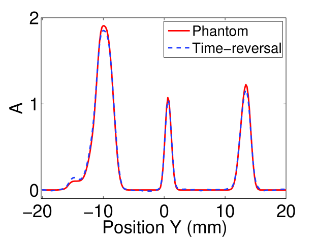
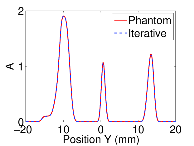
Figure 4: (a) and (c) are reconstructed images from noiseless data with full-view scanning geometry by use of the TR method and iterative method, respectively. (b) and (d) are the corresponding profiles along the ‘Y’-axis indicated in panel (a).

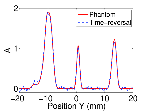
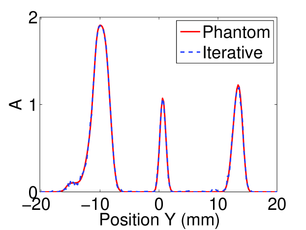
Figure 5: (a) and (c) are reconstructed images from the noisy pressure data with 3% AWGN corresponding to the full-view scanning geometry by use of the TR method and iterative method, respectively. (b) and (d) are the corresponding profiles.

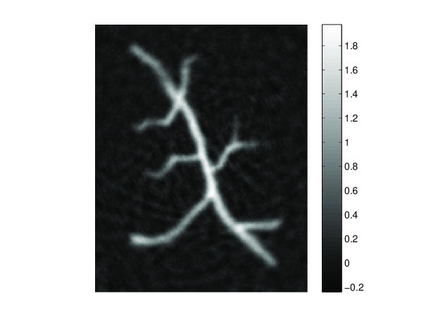
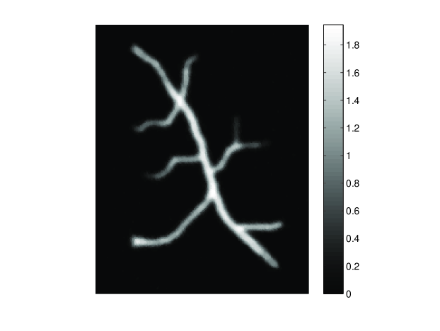
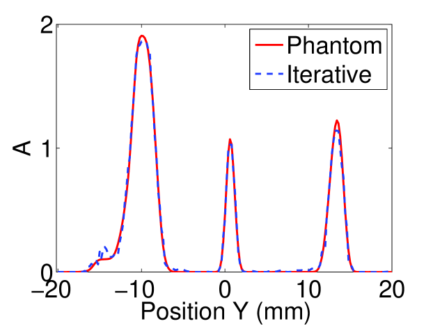
Figure 6: (a) and (c) are reconstructed images from the noisy pressure data with 3% AWGN corresponding to the few-view scanning geometry by use of the TR method and iterative method, respectively. (b) and (d) are the corresponding profiles.

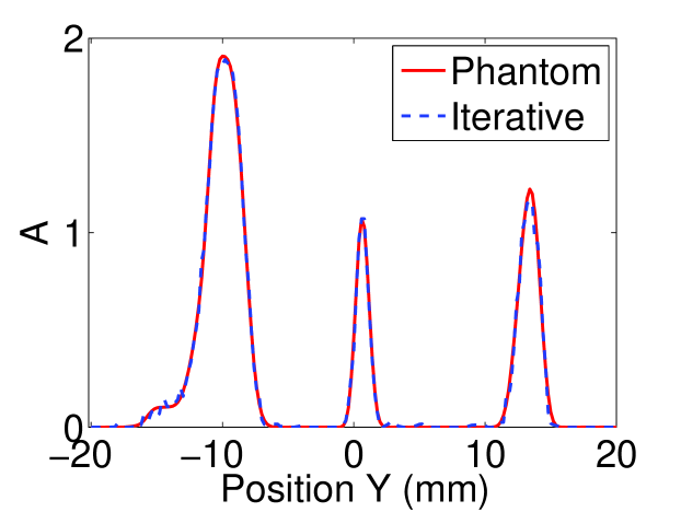
Figure 7: (a) and (c) are reconstructed images from the noisy pressure data with 3% AWGN corresponding to the limited-view scanning geometry by use of the TR method and iterative method, respectively. (b) and (d) are the corresponding profiles.

V-B Simulation results with errors in SOS and density maps

Figure 8 shows the images reconstructed from noisy pressure data corresponding to the low contrast disc phantom in the case where SOS and density maps have no error. The results corresponding to TR and iterative image reconstruction algorithms are shown in the top and bottom row, respectively. The RMSE corresponding to the time-reversal and the iterative results are 0.026 and 0.007, respectively. These results suggest that the iterative algorithm can more effectively reduce the noise level in the reconstructed images than the time-reversal algorithm.

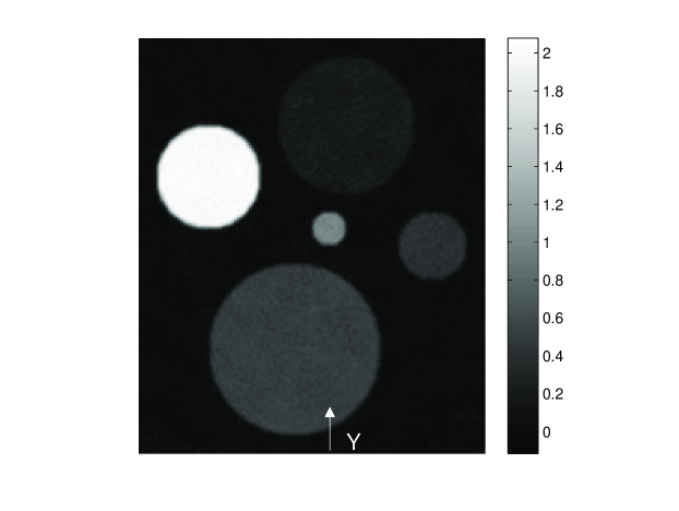
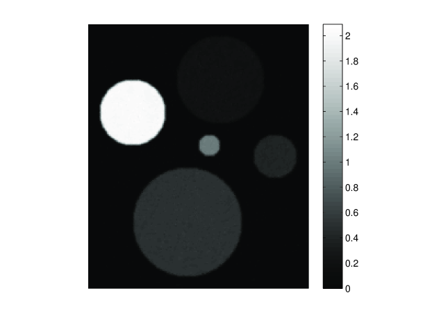
Figure 8: (a) and (c) are reconstructed images with actual SOS and density maps by use of the TR method and iterative method, respectively. (b) and (d) are the corresponding profiles along the ‘Y’-axis indicated in panel (a).

The images reconstructed by use of the SOS and density maps with errors are shown in Fig. 9. The image produced by the iterative method has cleaner background than the TR result, and the RMSE corresponding to the TR and the iterative results are 0.086 and 0.034, respectively. The boundaries of the disc phantoms also appear sharper in the image reconstructed by the iterative method as compared to the TR result. This can be attributed to the TV regularization employed in the iterative method. These results suggest that appropriately regularized iterative reconstruction methods can be more robust to the errors in the SOS and density maps than the TR method.

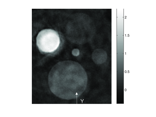
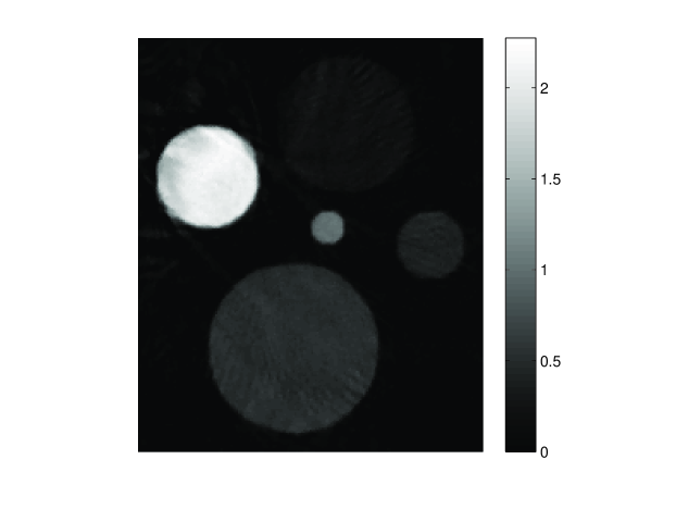
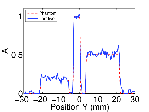
Figure 9: (a) and (c) are reconstructed images with SOS and density maps with errors by use of the TR method and iterative method, respectively. (b) and (d) are the corresponding profiles along the ‘Y’-axis indicated in panel (a).

V-C 3D simulation results

The 3D blood vessel phantom and the reconstructed images were visualized by the maximum intensity projection (MIP) method. Figure 10-(a) shows the phantom image, and Fig. 10-(b) and (c) display the images reconstructed by use of the TR method and the iterative method, respectively. They are all displayed in the same grey scale window. The RMSE corresponding to the TR and the iterative results are 0.018 and 0.003, respectively. These results suggest that the iterative method is robust to the data incompleteness and the noise in the pressure data. The computational time of the TR method was approximately 6 minutes, while the iterative method with 10 iterations required 110 minutes.

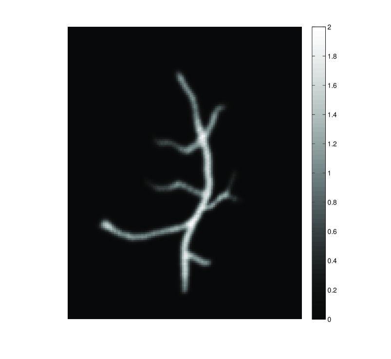
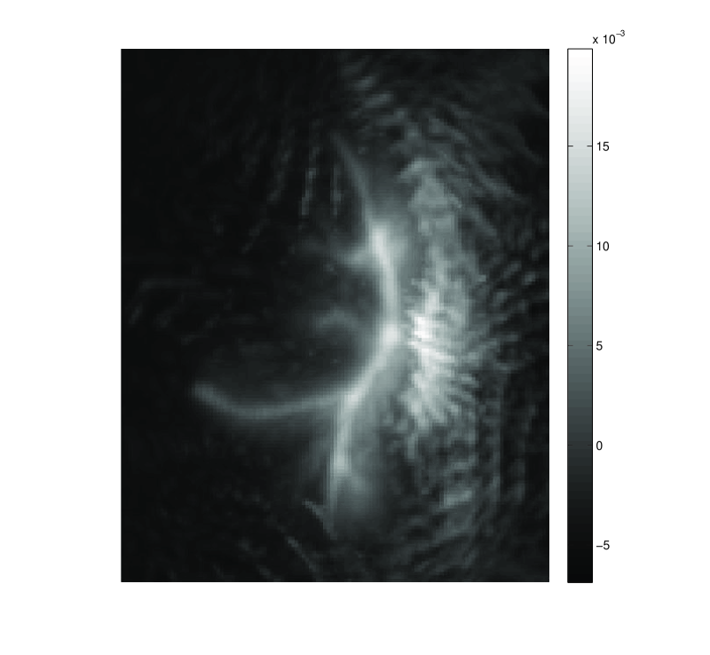
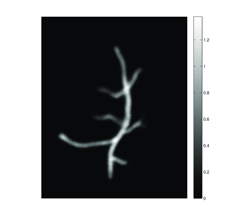
Figure 10: Maximum intensity projection renderings of the 3D phantom (a), and the reconstructed 3D images by use of the TR method (b) and the iterative method (c).

V-D Experimental results

The images reconstructed from the experimental data are shown in Figs. 11 - 14. Figure 11 shows the image reconstructed with the full-view scanning geometry by use of the TR method (top row) and the iterative method (bottom row). Figure 11-(a) and (c) display the reference images produced by each of the methods when the acrylic shell was absent. Figure 11-(b) and (e) show the reconstructed images for the case when the acrylic shell was present. The RMSE between Fig. 11-(b), (d) and the reference images 11-(a), (c) are 0.003 and 0.002, respectively. Figure 12-(a) and (c) show the images reconstructed with the few-view scanning geometry when the acrylic shell was present. The corresponding image profiles are displayed in Figure 12-(b) and (d). The profiles of Fig. 12-(a) and (c) along the ‘Y’-axis were shown in Fig. 13, which shows that the iterative method produced higher resolution images than the TR method. This can be attritubed to the TV regularization that mitigates model errors that arise, for example, by neglecting the shear wave and finite transducer aperture effects. The RMSE between Fig. 12-(b), (d) and their reference images are 0.005 and 0.002, , respectively. Figure 14 displays the images reconstructed with the limited-view scanning geometry when the acrylic shell was present. The RMSE between Fig. 14-(a), (c) and their reference images are 0.007 and 0.003, respectively. These results show that the iterative algorithm can effectively compensate for the acoustic attenuation and mitigate artifacts and distortions due to incomplete measurement data.

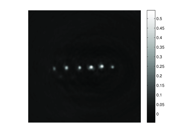
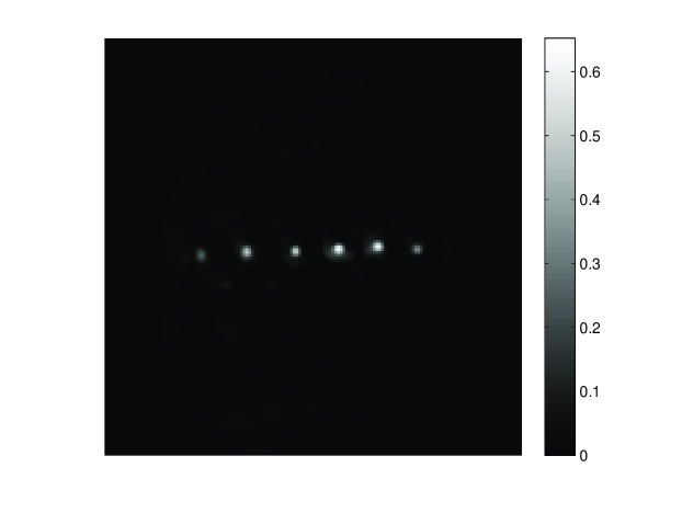
Figure 11: (a) and (b) are reconstructed images by use of the TR method from 200 views with acrylic shell absent and present, respectively. (c) and (d) are reconstructed images by use of the iterative method from 200 views with acrylic shell absent and present, respectively.

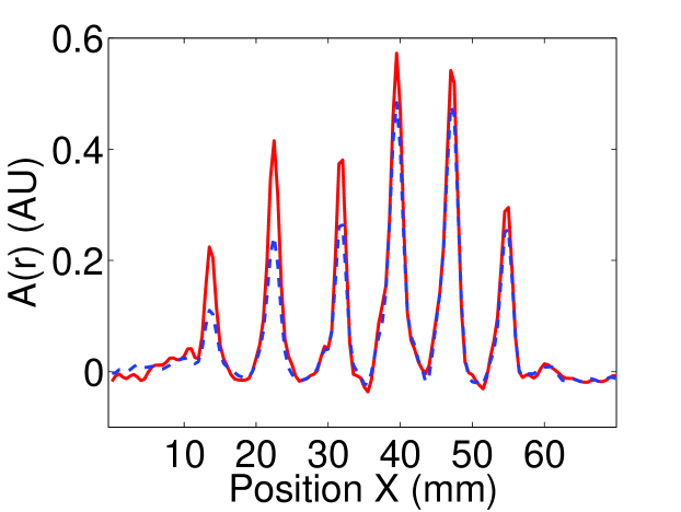
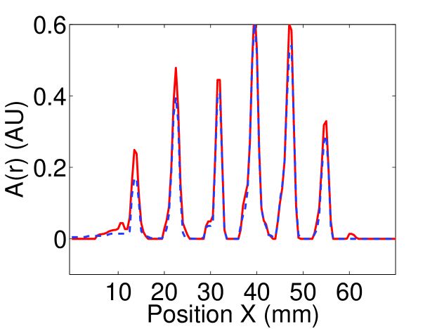
Figure 12: (a) and (c) are reconstructed images with data from 50 view angles over 360 degrees (acrylic shell present) by use of the TR method and iterative method, respectively. (b) and (d) are their corresponding profiles (dashed blue lines), where red solid lines are the profiles of the reference images in Fig. 11 (a) and (c).

Figure 13: The profiles of the reconstructed images in Fig. 12 along the ‘Y’-axis indicated in Fig. 12(a).

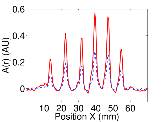
Figure 14: (a) and (c) are reconstructed images with data from 100 view angles over 180 degrees (acrylic shell present) by use of the TR method and iterative method, respectively. (b) and (d) are their corresponding profiles (dashed blue lines), where red solid lines are the profiles of the reference images in Fig. 11 (a) and (c).

VI Conclusion and discussion

We proposed and investigated a full-wave approach to iterative image reconstruction in PACT with acoustically inhomogeneous lossy media. An explicit formulation of the discrete imaging model based on the k-space pseudospectral method was described, and the details of implementing the forward and backprojection operators were provided. The matched operator pair was employed in an iterative image reconstruction algorithm that sought to minimize a TV-regularized PLS cost function. The developed reconstruction methodology was investigated by use of both computer-simulated and experimental PACT measurement data, and the results demonstrated that the reconstruction methodology can effectively mitigate image artifacts due to data incompleteness, noise, finite sampling, and modeling errors. This suggests that the proposed image reconstruction method has the potential to be adopted in preclinical and clinical PACT applications.

There remain several important topics to further investigate and validate the proposed iterative reconstruction method. It has been shown [20, 23] that the performance of reconstruction methods can be degraded when the SOS distribution satisfies a trapping condition [20, 23]. Therefore, future studies may include the investigation of numerical properties of the proposed image reconstruction method for cases in which the SOS distribution satisfies the trapping condition. Also, because the signal detectability is affected by the noise properties of an image reconstruction method, investigation of statistical properties of the iterative image reconstruction method is another important topic for future studies. Moreover, the proposed image reconstruction method can be further validated through additional experimental studies, and the quality of the produced images will be assessed by use of objective and quantitative measures.

acknowledments

This research was supported by NIH award EB010049.

appendix-A: Modeling transducer impulse responses

An important feature of the proposed discrete PACT imaging model is that the transducer’s impulse responses, including the spatial impulse response (SIR) and the acousto-electrical impulse response (EIR), can be readily incorporated into the system matrix.

The SIR accounts for the averaging effect over the transducer surface [50, 51, 52], which can be described as

$$\hat{p}^{\text{SIR}}(\mathbf{r}_{l}^{d},m\Delta t)=\frac{\int_{S(\mathbf{r}_{l}^{d})}\mathrm{d}S(\mathbf{r}^{\prime}_{l})p(\mathbf{r}^{\prime}_{l},m\Delta t)}{S(\mathbf{r}_{l}^{d})},$$ (45)

where $\hat{p}^{\text{SIR}}(\mathbf{r}_{l}^{d},m\Delta t)$ is the averaged pressure at time $t=m\Delta t$ over the surface of the $l$-th transducer, $S(\mathbf{r}_{l}^{d})$ is the surface area of the $l$-th transducer centered at $\mathbf{r}_{l}^{d}$.

In order to incorporate the SIR into the system matrix, we can divide the transducer surface into $K$ small patches with equal area $\Delta S$ that is much less than the acoustic wavelength, so the integral in Eqn. 45 can be approximated by summation as

$$\hat{p}^{\text{SIR}}(\mathbf{r}_{l}^{d},m\Delta t)\simeq\sum\limits_{k=1}^{K}p(\mathbf{r}^{k}_{l},m\Delta t)\frac{\Delta S}{S(\mathbf{r}_{l}^{d})},$$ (46)

or in the equivalent matrix form

$$\hat{p}^{\text{SIR}}(\mathbf{r}_{l}^{d},m\Delta t)\simeq\boldsymbol{\gamma}^{\text{SIR}}\hat{\mathbf{p}}_{m}^{l}$$ (47)

where $\mathbf{r}^{k}_{l}$ denotes the center of the $k$-th patch of the $l$-th transducer, $\Delta S$ is the patch area, $\boldsymbol{\gamma}^{\text{SIR}}\equiv\frac{\Delta S}{S(\mathbf{r}_{l}^{d})}(1,\cdots,1)$ is a $1\times K$ vector, $\hat{\mathbf{p}}_{m}^{l}=(p(\mathbf{r}^{1}_{l},m\Delta t),\cdots,p(\mathbf{r}^{K}_{l},m\Delta t))^{\rm T}$ denotes the acoustic pressure at patches of $l$-th transducer at time $m\Delta t$. Here for simplicity, we assume all the transducers are divided into $K$ patches with equal area $\Delta S$, and it is readily to extend to general cases where $l$-th transducer is divided into $K_{l}$ patches with area of $\Delta S_{lk}$.

Recalling the measured pressure data $\hat{\mathbf{p}}_{m}$ and $\hat{\mathbf{p}}$ defined for point-like transducer, we can redefine $\hat{\mathbf{p}}_{m}$ as a $KL\times 1$ vector that represents the acoustic pressure at patches of transducers with finite area at time $t=m\Delta t$ as

$$\hat{\mathbf{p}}_{m}\equiv\begin{bmatrix}\hat{\mathbf{p}}_{m}^{1}\\ \vdots\\ \hat{\mathbf{p}}_{m}^{L}\end{bmatrix}.$$ (48)

The corresponding $\hat{\mathbf{p}}$ can be redefine as a $KLM\times 1$ vector denoting the measured pressure data corresponding to all transducer and temporal samples as

$$\hat{\mathbf{p}}\equiv\begin{bmatrix}\hat{\mathbf{p}}_{0}\\ \vdots\\ \hat{\mathbf{p}}_{M-1}\end{bmatrix}.$$ (49)

The averaged pressure measured by all transducer and temporal samples can be defined as the $LM\times 1$ vector

$$\hat{\mathbf{p}}^{\text{SIR}}\equiv\begin{bmatrix}\hat{\mathbf{p}}_{0}^{\text{SIR}}\\ \vdots\\ \hat{\mathbf{p}}_{M-1}^{\text{SIR}}\end{bmatrix}.$$ (50)

where the $L\times 1$ vector

$$\hat{\mathbf{p}}_{m}^{\text{SIR}}\equiv\begin{bmatrix}\hat{p}^{\text{SIR}}(\mathbf{r}_{1}^{d},m\Delta t)\\ \vdots\\ \hat{p}^{\text{SIR}}(\mathbf{r}_{L}^{d},m\Delta t)\end{bmatrix}.$$ (51)

According to Eqn. 47, $\hat{\mathbf{p}}$ and $\hat{\mathbf{p}}^{\text{SIR}}$ can be related as

$$\hat{\mathbf{p}}^{\text{SIR}}=\boldsymbol{\Gamma}^{\text{SIR}}\hat{\mathbf{p}}$$ (52)

where the $KLM\times LM$ matrix

$$\boldsymbol{\Gamma}^{\text{SIR}}\equiv\begin{bmatrix}\boldsymbol{\gamma}^{\text{SIR}}&\mathbf{0}_{1\times K}&\cdots&\mathbf{0}_{1\times K}\\ \mathbf{0}_{1\times K}&\boldsymbol{\gamma}^{\text{SIR}}&\cdots&\mathbf{0}_{1\times K}\\ \vdots&\vdots&\ddots&\vdots\\ \mathbf{0}_{1\times K}&\mathbf{0}_{1\times K}&\cdots&\boldsymbol{\gamma}^{\text{SIR}}\end{bmatrix}.$$ (53)

The EIR models the electrical response of the piezoelectric transducer. With the assumption that the transducer is a linear shift invariant system with respect to the input averaged pressure time sequence, the output voltage signal is the convolution result of the input and the EIR.

For simplicity, the transducers are assumed to process identical EIR, and let $\mathbf{h}^{e}=(h_{1}^{e},\cdots,h_{J}^{e})^{\rm T}$ be the discrete samples of the EIR. The input averaged pressure time sequence of the $l$-th transducer can be defined as a $L\times 1$ vector $\hat{\mathbf{p}}^{l}_{\text{SIR}}\equiv(\hat{p}^{\text{SIR}}(\mathbf{r}_{l}^{d},0),\cdots,\hat{p}^{\text{SIR}}(\mathbf{r}_{l}^{d},(M-1)\Delta t))^{\rm T}$. Then the output voltage signal $\hat{\mathbf{p}}_{l}^{\text{IR}}$ of the $l$-th transducer can be expressed as a $(J+M-1)\times 1$ vector

$$\hat{\mathbf{p}}_{l}^{\text{IR}}=\mathbf{h}^{e}*\hat{\mathbf{p}}^{l}_{\text{SIR}},$$ (54)

where $*$ denotes discrete linear convolution operation, which can be constructed as a matrix multiplication by converting one of the operands into the corresponding Toeplitz matrix.

The output voltage signals of all transducers $\hat{\mathbf{p}}^{\text{IR}}\equiv(\hat{\mathbf{p}}_{1}^{\text{IR}},\cdots,\hat{\mathbf{p}}_{L}^{\text{IR}})^{\rm T}$ can then be computed as

$$\hat{\mathbf{p}}^{\text{IR}}=\boldsymbol{\Gamma}^{\text{EIR}}\hat{\mathbf{p}}^{\text{SIR}}$$ (55)

where the $L(J+M-1)\times LM$ matrix

$$\boldsymbol{\Gamma}^{\text{EIR}}\equiv\begin{bmatrix}\boldsymbol{\gamma}^{\text{EIR}}\\ \vdots\\ \boldsymbol{\gamma}^{\text{EIR}}\end{bmatrix}$$ (56)

and $\boldsymbol{\gamma}^{\text{EIR}}$ is a $(J+M-1)\times LM$ Toeplitz-like matrix defined as

$$\boldsymbol{\gamma}^{\text{EIR}}\equiv\begin{bmatrix}h_{1}^{e}&\mathbf{0}_{1\times(L-1)}&0&\cdots&0&\mathbf{0}_{1\times(L-1)}&0\\ \vdots&\vdots&h_{1}^{e}&\vdots&\vdots&\vdots&\vdots\\ h_{J}^{e}&\vdots&\vdots&\vdots&0&\mathbf{0}_{1\times(L-1)}&0\\ 0&\mathbf{0}_{1\times(L-1)}&h_{J}^{e}&\cdots&h_{1}^{e}&\mathbf{0}_{1\times(L-1)}&0\\ 0&\mathbf{0}_{1\times(L-1)}&0&\cdots&\vdots&\vdots&h_{1}^{e}\\ \vdots&\vdots&\vdots&\vdots&h_{J}^{e}&\vdots&\vdots\\ 0&\mathbf{0}_{1\times(L-1)}&0&\cdots&0&\mathbf{0}_{1\times(L-1)}&h_{J}^{e}\end{bmatrix}$$ (57)

By use of Eqns. (36), (52), and (55), it is readily found that

$$\hat{\mathbf{p}}^{\text{IR}}=\boldsymbol{\Gamma}^{\text{EIR}}\boldsymbol{\Gamma}^{\text{SIR}}\mathbf{S}\mathbf{T}_{M-1}\cdots\mathbf{T}_{1}\mathbf{T}_{0}\mathbf{p}_{0},$$ (58)

and the corresponding system matrix that incorporates the transducer impulse responses is found to be

$$\mathbf{H}^{\text{IR}}\equiv\boldsymbol{\Gamma}^{\text{EIR}}\boldsymbol{\Gamma}^{\text{SIR}}\mathbf{S}\mathbf{T}_{M-1}\cdots\mathbf{T}_{1}\mathbf{T}_{0}.$$ (59)

appendix-B: Implementation of the FISTA algorithm for PACT

Equation (43) was solved iteratively whose pseudocodes are provided in Alg. 1, where ‘Lip’ is the Lipschitz constant of the operator $2\mathbf{H}^{\rm T}\mathbf{H}$ [42].

Algorithm 1 Solver of the optimization problem defined by Eqn. (43)

0:  $\hat{\mathbf{p}}$, $\mathbf{p}_{0}^{(0)}$, $\lambda$, $\rm Lip$

0:  $\hat{\mathbf{p}}_{0}$

1:  $t^{(0)}\leftarrow 1$; $\boldsymbol{\sigma}_{0}^{(1)}\leftarrow\mathbf{p}_{0}^{(0)}$ {Set the initial guess (The zero initial guess was employed in all the studies in this article)}

2:  for $\zeta=1$ to $Z$ do

3:        $\mathbf{p}_{0}^{(\zeta)}\leftarrow\rm{F\_Dnoise}\big{(}\boldsymbol{\sigma}_{0}^{(\zeta)}-\frac{2}{\rm Lip}\mathbf{H}^{T}(\mathbf{H}\boldsymbol{\sigma}_{0}^{(\zeta)}-\hat{\mathbf{p}}),{2\lambda}/{Lip}\big{)}$

4:        $t^{(\zeta+1)}\leftarrow 0.5+0.5\sqrt{1+4(t^{(\zeta)})^{2}}$

5:        $\boldsymbol{\sigma}_{0}^{(\zeta+1)}\leftarrow\mathbf{p}_{0}^{(\zeta)}+(t^{(\zeta)}-1)(\mathbf{p}_{0}^{(\zeta)}-\mathbf{p}_{0}^{(\zeta-1)})/t^{(\zeta+1)}$

6:  end for

7:  $\hat{\mathbf{p}}_{0}\leftarrow\mathbf{p}_{0}^{(Z)}$

Note that we extended the FISTA algorithm described in Ref. [42] to 3D. The function ‘F_Dnoise’ in Alg. 1-Line 3 solves a de-noising problem defined as:

$$\hat{\mathbf{x}}=\arg\min_{\mathbf{x}\geq 0}\lVert\mathbf{y}-\mathbf{x}\rVert^{2}+\beta|\mathbf{x}|_{\rm TV},$$ (60)

where $\beta=2\lambda/{\rm Lip}$ and

$$\mathbf{y}=\hat{\mathbf{p}}-\frac{2}{\rm Lip}\mathbf{H}^{\rm T}(\mathbf{H}\boldsymbol{\sigma}_{0}^{(\zeta)}-\hat{\mathbf{p}}).$$ (61)

It has been demonstrated that Eqn. (60) can be solved efficiently [42], and the pseudocodes are provided in Alg. 2.

Algorithm 2 Solver of the de-noising problem defined by Eqn. (60)

0:  $\mathbf{y}$, $\beta$

0:  $\hat{\mathbf{x}}$

1:  $\big{[}\mathbf{a}^{(1)},\mathbf{b}^{(1)},\mathbf{c}^{(1)}\big{]}\leftarrow$ $\big{[}\mathbf{0}_{(N_{1}-1)\times N_{2}\times N_{3}},\mathbf{0}_{N_{1}\times(N_{2}-1)\times N_{3}},\mathbf{0}_{N_{1}\times N_{2}\times(N_{3}-1)}\big{]}$$\big{[}\mathbf{d}^{(0)},\mathbf{e}^{(0)},\mathbf{f}^{(0)}\big{]}\leftarrow$ $\big{[}\mathbf{0}_{(N_{1}-1)\times N_{2}\times N_{3}},\mathbf{0}_{N_{1}\times(N_{2}-1)\times N_{3}},\mathbf{0}_{N_{1}\times N_{2}\times(N_{3}-1)}\big{]}$$t^{(1)}=1$

2:  for $\zeta=1$ to $Z$ do

3:        $\big{[}\mathbf{d}^{(\zeta)},\mathbf{e}^{(\zeta)},\mathbf{f}^{(\zeta)}\big{]}\leftarrow\mathcal{P}_{p}\Big{\{}[\mathbf{a}^{(\zeta)},\mathbf{b}^{(\zeta)},\mathbf{c}^{(\zeta)}]+(6\beta)^{-1}\mathcal{P}_{l}^{T}\big{\{}\mathcal{P}_{c}\{\mathbf{y}-0.5\beta\mathcal{P}_{l}\{\mathbf{a}^{(\zeta)},\mathbf{b}^{(\zeta)},\mathbf{c}^{(\zeta)}\}\}\big{\}}\Big{\}}$

4:        $t^{(\zeta+1)}\leftarrow 1+0.5\sqrt{1+4(t^{(\zeta)})^{2}}$

5:        $\big{[}\mathbf{a}^{(\zeta+1)},\mathbf{b}^{(\zeta+1)},\mathbf{c}^{(\zeta+1)}\big{]}\leftarrow(t^{(\zeta)}-1)/t^{(\zeta+1)}\big{[}\mathbf{d}^{(\zeta)}-\mathbf{d}^{(\zeta-1)},\mathbf{e}^{(\zeta)}-\mathbf{e}^{(\zeta-1)},\mathbf{f}^{(\zeta)}-\mathbf{f}^{(\zeta-1)}\big{]}$

6:  end for

7:  $\hat{\mathbf{x}}\leftarrow\mathcal{P}_{c}\big{\{}\mathbf{y}-\lambda\mathcal{P}_{l}\{\mathbf{d}^{(Z)},\mathbf{e}^{(Z)},\mathbf{f}^{(Z)}\}\big{\}}$

The four operators $\mathcal{P}_{l}$ $\mathcal{P}_{c}$, $\mathcal{P}_{l}^{T}$ and $\mathcal{P}_{p}$ in Alg. 2 are defined as follows:

$\mathcal{P}_{l}:\mathbb{R}^{(N_{1}-1)\times N_{2}\times N_{3}}\times\mathbb{R}^{N_{1}\times(N_{2}-1)\times N_{3}}\times\mathbb{R}^{N_{1}\times N_{2}\times(N_{3}-1)}\rightarrow\mathbb{R}^{N_{1}\times N_{2}\times N_{3}}$.

$$\begin{split}&\big{[}\mathcal{P}_{l}\{\mathbf{a},\mathbf{b},\mathbf{c}\}\big{]}_{n_{1},n_{2},n_{3}}=\\ &[\mathbf{a}]_{n_{1},n_{2},n_{3}}+[\mathbf{b}]_{n_{1},n_{2},n_{3}}+[\mathbf{c}]_{n_{1},n_{2},n_{3}}-\\ &[\mathbf{a}]_{n_{1}-1,n_{2},n_{3}}-[\mathbf{b}]_{n_{1},n_{2}-1,n_{3}}-[\mathbf{c}]_{n_{1},n_{2},n_{3}-1}\\ &\text{for}\quad n_{1}=1,\cdots,N_{1},\,n_{2}=1,\cdots,N_{2},\,n_{3}=1,\cdots,N_{3},\end{split}$$ (62)

where we assume $[\mathbf{a}]_{0,n_{2},n_{3}}=[\mathbf{a}]_{N_{1},n_{2},n_{3}}=[\mathbf{b}]_{n_{1},0,n_{3}}=[\mathbf{b}]_{n_{1},N_{2},n_{3}}=[\mathbf{c}]_{n_{1},n_{2},0}=[\mathbf{c}]_{n_{1},n_{2},N_{3}}\equiv 0$.

$\mathcal{P}_{c}:\mathbb{R}^{N_{1}\times N_{2}\times N_{3}}\rightarrow\mathbb{R}^{N_{1}\times N_{2}\times N_{3}}$.

$$\big{[}\mathcal{P}_{c}\{\mathbf{x}\}\big{]}_{n_{1},n_{2},n_{3}}=\max\big{\{}0,[\mathbf{x}]_{n_{1},n_{2},n_{3}}.\big{\}}$$ (63)

$\mathcal{P}_{l}^{T}:\mathbb{R}^{N_{1}\times N_{2}\times N_{3}}\rightarrow\mathbb{R}^{(N_{1}-1)\times N_{2}\times N_{3}}\times\mathbb{R}^{N_{1}\times(N_{2}-1)\times N_{3}}\times\mathbb{R}^{N_{1}\times N_{2}\times(N_{3}-1)}$. If we denote the input and output matrices by $\mathbf{y}$ and $(\mathbf{a},\mathbf{b},\mathbf{c})$ respectively, we have

$$\begin{split}&[\mathbf{a}]_{n_{1},n_{2},n_{3}}=[\mathbf{y}]_{n_{1},n_{2},n_{3}}-[\mathbf{y}]_{n_{1}+1,n_{2},n_{3}},\\ &\text{for}\quad n_{1}=1,\cdots,N_{1}-1,n_{2}=1,\cdots,N_{2},n_{3}=1,\cdots,N_{3}\\ &[\mathbf{b}]_{n_{1},n_{2},n_{3}}=[\mathbf{y}]_{n_{1},n_{2},n_{3}}-[\mathbf{y}]_{n_{1},n_{2}+1,n_{3}},\\ &\text{for}\quad n_{1}=1,\cdots,N_{1},n_{2}=1,\cdots,N_{2}-1,n_{3}=1,\cdots,N_{3}\\ &[\mathbf{c}]_{n_{1},n_{2},n_{3}}=[\mathbf{y}]_{n_{1},n_{2},n_{3}}-[\mathbf{y}]_{n_{1},n_{2},n_{3}+1},\\ &\text{for}\quad n_{1}=1,\cdots,N_{1},n_{2}=1,\cdots,N_{2},n_{3}=1,\cdots,N_{3}-1.\end{split}$$ (64)

$\mathcal{P}_{p}:\mathbb{R}^{(N_{1}-1)\times N_{2}\times N_{3}}\times\mathbb{R}^{N_{1}\times(N_{2}-1)\times N_{3}}\times\mathbb{R}^{N_{1}\times N_{2}\times(N_{3}-1)}\rightarrow\mathbb{R}^{(N_{1}-1)\times N_{2}\times N_{3}}\times\mathbb{R}^{N_{1}\times(N_{2}-1)\times N_{3}}\times\mathbb{R}^{N_{1}\times N_{2}\times(N_{3}-1)}$. If we denote the input and output matrices by $(\mathbf{a},\mathbf{b},\mathbf{c})$ and $(\mathbf{d},\mathbf{e},\mathbf{f})$ respectively, we have

$$\begin{split}[\mathbf{d}]_{n_{1},n_{2},n_{3}}=\frac{[\mathbf{a}]_{n_{1},n_{2},n_{3}}}{\max\big{\{}1,\sqrt{[\mathbf{a}]^{2}_{n_{1},n_{2},n_{3}}+[\mathbf{b}]^{2}_{n_{1},n_{2},n_{3}}+[\mathbf{c}]^{2}_{n_{1},n_{2},n_{3}}}\big{\}}}\\ [\mathbf{e}]_{n_{1},n_{2},n_{3}}=\frac{[\mathbf{b}]_{n_{1},n_{2},n_{3}}}{\max\big{\{}1,\sqrt{[\mathbf{a}]^{2}_{n_{1},n_{2},n_{3}}+[\mathbf{b}]^{2}_{n_{1},n_{2},n_{3}}+[\mathbf{c}]^{2}_{n_{1},n_{2},n_{3}}}\big{\}}}\\ [\mathbf{f}]_{n_{1},n_{2},n_{3}}=\frac{[\mathbf{c}]_{n_{1},n_{2},n_{3}}}{\max\big{\{}1,\sqrt{[\mathbf{a}]^{2}_{n_{1},n_{2},n_{3}}+[\mathbf{b}]^{2}_{n_{1},n_{2},n_{3}}+[\mathbf{c}]^{2}_{n_{1},n_{2},n_{3}}}\big{\}}},\end{split}$$ (65)

where $n_{1}=1,\cdots,N_{1}$, $n_{2}=1,\cdots,N_{2}$, $n_{3}=1,\cdots,N_{3}$, and we assume $[\mathbf{a}]_{0,n_{2},n_{3}}=[\mathbf{a}]_{N_{1},n_{2},n_{3}}=[\mathbf{b}]_{n_{1},0,n_{3}}=[\mathbf{b}]_{n_{1},N_{2},n_{3}}=[\mathbf{c}]_{n_{1},n_{2},0}=[\mathbf{c}]_{n_{1},n_{2},N_{3}}\equiv 0$.

References

- [1] L. V. Wang, “Photoacoustic imaging and spectroscopy,” in Photoacoustic Imaging and Spectroscopy. CRC, 2009.
- [2] A. A. and A. A. Karabutov, “Optoacoustic tomography,” in Biomedical Photonics Handbook, T. Vo-Dinh, Ed. CRC Press LLC, 2003.
- [3] M. Xu and L. V. Wang, “Photoacoustic imaging in biomedicine,” Review of Scientific Instruments, vol. 77, no. 041101, 2006.
- [4] Z. Xu, C. Li, and L. V. Wang, “Photoacoustic tomography of water in phantoms and tissue,” Journal of Biomedical Optics, vol. 15, no. 3, pp. 036 019–036 019–6, 2010. [Online]. Available: + http://dx.doi.org/10.1117/1.3443793
- [5] V. E. Gusev and A. A. Karabutov, “Laser optoacoustic,” in Laser Optoacoustic. AIP, 1993.
- [6] R. Kruger, D. Reinecke, and G. Kruger, “Thermoacoustic computed tomography- technical considerations,” Medical Physics, vol. 26, pp. 1832–1837, 1999.
- [7] M. Haltmeier, O. Scherzer, P. Burgholzer, and G. Paltauf, “Thermoacoustic computed tomography with large planar receivers,” Inverse Problems, vol. 20, no. 5, pp. 1663–1673, 2004. [Online]. Available: http://stacks.iop.org/0266-5611/20/1663
- [8] B. T. Cox, S. R. Arridge, K. P. Köstli, and P. C. Beard, “Two-dimensional quantitative photoacoustic image reconstruction of absorption distributions in scattering media by use of a simple iterative method,” Appl. Opt., vol. 45, no. 8, pp. 1866–1875, Mar 2006. [Online]. Available: http://ao.osa.org/abstract.cfm?URI=ao-45-8-1866
- [9] Z. Xu, Q. Zhu, and L. V. Wang, “In vivo photoacoustic tomography of mouse cerebral edema induced by cold injury,” Journal of Biomedical Optics, vol. 16, no. 6, pp. 066 020–066 020–4, 2011. [Online]. Available: + http://dx.doi.org/10.1117/1.3584847
- [10] C. Huang, L. Nie, R. W. Schoonover, Z. Guo, C. O. Schirra, M. A. Anastasio, and L. V. Wang, “Aberration correction for transcranial photoacoustic tomography of primates employing adjunct image data,” Journal of Biomedical Optics, vol. 17, no. 6, p. 066016, 2012. [Online]. Available: http://link.aip.org/link/?JBO/17/066016/1
- [11] F. J. Fry and J. E. Barger, “Acoustical properties of the human skull,” The Journal of the Acoustical Society of America, vol. 63, no. 5, pp. 1576–1590, 1978. [Online]. Available: http://dx.doi.org/doi/10.1121/1.381852
- [12] X. Jin, C. Li, and L. V. Wang, “Effects of acoustic heterogeneities on transcranial brain imaging with microwave-induced thermoacoustic tomography,” Medical Physics, vol. 35, no. 7, pp. 3205–3214, 2008. [Online]. Available: http://dx.doi.org/10.1118/1.2938731
- [13] C. Huang, L. Nie, R. W. Schoonover, L. V. Wang, and M. A. Anastasio, “Photoacoustic computed tomography correcting for heterogeneity and attenuation,” Journal of Biomedical Optics, vol. 17, no. 6, p. 061211, 2012. [Online]. Available: http://link.aip.org/link/?JBO/17/061211/1
- [14] Y. Xu and L. Wang, “Effects of acoustic heterogeneity in breast thermoacoustic tomography,” Ultrasonics, Ferroelectrics and Frequency Control, IEEE Transactions on, vol. 50, no. 9, pp. 1134 –1146, sept. 2003.
- [15] D. Modgil, M. A. Anastasio, and P. J. La Rivière, “Image reconstruction in photoacoustic tomography with variable speed of sound using a higher-order geometrical acoustics approximation,” Journal of Biomedical Optics, vol. 15, no. 2, pp. 021 308–021 308–9, 2010. [Online]. Available: + http://dx.doi.org/10.1117/1.3333550
- [16] J. Jose, R. G. H. Willemink, S. Resink, D. Piras, J. C. G. van Hespen, C. H. Slump, W. Steenbergen, T. G. van Leeuwen, and S. Manohar, “Passive element enriched photoacoustic computed tomography (per pact) for simultaneous imaging of acoustic propagation properties and light absorption,” Opt. Express, vol. 19, no. 3, pp. 2093–2104, Jan 2011. [Online]. Available: http://www.opticsexpress.org/abstract.cfm?URI=oe-19-3-2093
- [17] X. L. Deán-Ben, V. Ntziachristos, and D. Razansky, “Statistical optoacoustic image reconstruction using a-priori knowledge on the location of acoustic distortions,” Applied Physics Letters, vol. 98, no. 17, p. 171110, 2011. [Online]. Available: http://link.aip.org/link/?APL/98/171110/1
- [18] Z. Yuan and H. Jiang, “Three-dimensional finite-element-based photoacoustic tomography: Reconstruction algorithm and simulations,” Medical Physics, vol. 34, no. 2, pp. 538–546, 2007. [Online]. Available: http://link.aip.org/link/?MPH/34/538/1
- [19] L. Yao and H. Jiang, “Enhancing finite element-based photoacoustic tomography using total variation minimization,” Appl. Opt., vol. 50, no. 25, pp. 5031–5041, Sep 2011. [Online]. Available: http://ao.osa.org/abstract.cfm?URI=ao-50-25-5031
- [20] Y. Hristova, P. Kuchment, and L. Nguyen, “Reconstruction and time reversal in thermoacoustic tomography in acoustically homogeneous and inhomogeneous media,” Inverse Problems, vol. 24, no. 5, p. 055006, 2008. [Online]. Available: http://stacks.iop.org/0266-5611/24/i=5/a=055006
- [21] B. E. Treeby, E. Z. Zhang, and B. T. Cox, “Photoacoustic tomography in absorbing acoustic media using time reversal,” Inverse Problems, vol. 26, no. 11, p. 115003, 2010. [Online]. Available: http://stacks.iop.org/0266-5611/26/i=11/a=115003
- [22] P. Stefanov and G. Uhlmann, “Thermoacoustic tomography with variable sound speed,” Inverse Problems, vol. 25, no. 7, p. 075011, 2009. [Online]. Available: http://stacks.iop.org/0266-5611/25/i=7/a=075011
- [23] J. Qian, P. Stefanov, G. Uhlmann, and H. Zhao, “An efficient neumann series-based algorithm for thermoacoustic and photoacoustic tomography with variable sound speed,” SIAM J. Img. Sci., vol. 4, no. 3, pp. 850–883, Sep. 2011. [Online]. Available: http://dx.doi.org/10.1137/100817280
- [24] B. T. Cox, S. Kara, S. R. Arridge, and P. C. Beard, “k-space propagation models for acoustically heterogeneous media: Application to biomedical photoacoustics,” The Journal of the Acoustical Society of America, vol. 121, no. 6, pp. 3453–3464, 2007. [Online]. Available: http://link.aip.org/link/?JAS/121/3453/1
- [25] T. Mast, L. Souriau, D.-L. Liu, M. Tabei, A. Nachman, and R. Waag, “A k-space method for large-scale models of wave propagation in tissue,” Ultrasonics, Ferroelectrics and Frequency Control, IEEE Transactions on, vol. 48, no. 2, pp. 341 –354, march 2001.
- [26] P. J. L. Rivière, J. Zhang, and M. A. Anastasio, “Image reconstruction in optoacoustic tomography for dispersive acoustic media,” Opt. Lett., vol. 31, no. 6, pp. 781–783, Mar 2006. [Online]. Available: http://ol.osa.org/abstract.cfm?URI=ol-31-6-781
- [27] P. Burgholzer, H. Grün, M. Haltmeier, R. Nuster, and G. Paltauf, “Compensation of acoustic attenuation for high-resolution photoacoustic imaging with line detectors,” Proceedings of the SPIE, vol. 6437, no. 1, p. 643724, 2007. [Online]. Available: http://dx.doi.org/doi/10.1117/12.700723
- [28] D. Modgil, M. A. Anastasio, and P. J. L. Riviere, “Photoacoustic image reconstruction in an attenuating medium using singular value decomposition,” Proceedings of the SPIE, vol. 7177, no. 1, p. 71771B, 2009. [Online]. Available: http://dx.doi.org/doi/10.1117/12.809030
- [29] X. L. Deán-Ben, D. Razansky, and V. Ntziachristos, “The effects of acoustic attenuation in optoacoustic signals,” Physics in Medicine and Biology, vol. 56, no. 18, p. 6129, 2011. [Online]. Available: http://stacks.iop.org/0031-9155/56/i=18/a=021
- [30] T. L. Szabo, “Time domain wave equations for lossy media obeying a frequency power law,” The Journal of the Acoustical Society of America, vol. 96, no. 1, pp. 491–500, 1994. [Online]. Available: http://dx.doi.org/doi/10.1121/1.410434
- [31] ——, “Diagnostic ultrasound imaging,” in Diagnostic Ultrasound Imaging: Inside Out. Elsevier, 2004.
- [32] P. M. Morse, “Theoretical acoustics,” in Theoretical Acoustics. Princeton University Press, 1987.
- [33] C. Huang, A. A. Oraevsky, and M. A. Anastasio, “Investigation of limited-view image reconstruction in optoacoustic tomography employing a priori structural information,” in Image Reconstruction from Incomplete Data VI, P. J. Bones, M. A. Fiddy, and R. P. Millane, Eds., vol. 7800, no. 1. SPIE, 2010, p. 780004. [Online]. Available: http://link.aip.org/link/?PSI/7800/780004/1
- [34] J.-F. Aubry, M. Tanter, M. Pernot, J.-L. Thomas, and M. Fink, “Experimental demonstration of noninvasive transskull adaptive focusing based on prior computed tomography scans,” The Journal of the Acoustical Society of America, vol. 113, no. 1, pp. 84–93, 2003. [Online]. Available: http://dx.doi.org/doi/10.1121/1.1529663
- [35] X. Jin and L. V. Wang, “Thermoacoustic tomography with correction for acoustic speed variations,” Physics in Medicine and Biology, vol. 51, no. 24, p. 6437, 2006. [Online]. Available: http://stacks.iop.org/0031-9155/51/i=24/a=010
- [36] J. Jose, R. G. H. Willemink, W. Steenbergen, C. H. Slump, T. G. van Leeuwen, and S. Manohar, “Speed-of-sound compensated photoacoustic tomography for accurate imaging,” Medical Physics, vol. 39, no. 12, pp. 7262–7271, 2012. [Online]. Available: http://link.aip.org/link/?MPH/39/7262/1
- [37] J. A. Fessler, “Penalized weighted least-squares reconstruction for positron emission tomography,” IEEE Transactions on Medical Imaging, vol. 13, pp. 290–300, 1994.
- [38] D. T. Lee and B. J. Schachter, “Two algorithms for constructing a delaunay triangulation,” International Journal of Parallel Programming, vol. 9, pp. 219–242, 1980, 10.1007/BF00977785. [Online]. Available: http://dx.doi.org/10.1007/BF00977785
- [39] B. Treeby and B. Cox, “k-wave: MATLAB toolbox for the simulation and reconstruction of photoacoustic wave fields,” Journal of Biomedical Optics, vol. 15, p. 021314, 2010.
- [40] M. Tabei, T. D. Mast, and R. C. Waag, “A k-space method for coupled first-order acoustic propagation equations,” The Journal of the Acoustical Society of America, vol. 111, no. 1, pp. 53–63, 2002. [Online]. Available: http://link.aip.org/link/?JAS/111/53/1
- [41] T. Katsibas and C. Antonopoulos, “A general form of perfectly matched layers for for three-dimensional problems of acoustic scattering in lossless and lossy fluid media,” Ultrasonics, Ferroelectrics and Frequency Control, IEEE Transactions on, vol. 51, no. 8, pp. 964 –972, aug. 2004.
- [42] A. Beck and M. Teboulle, “Fast gradient-based algorithms for constrained total variation image denoising and deblurring problems,” Image Processing, IEEE Transactions on, vol. 18, no. 11, pp. 2419 –2434, nov. 2009.
- [43] K. Wang, R. Su, A. A. Oraevsky, and M. A. Anastasio, “Investigation of iterative image reconstruction in three-dimensional optoacoustic tomography,” Physics in Medicine and Biology, vol. 57, no. 17, p. 5399, 2012. [Online]. Available: http://stacks.iop.org/0031-9155/57/i=17/a=5399
- [44] B. Zhang, S. Xu, F. Zhang, Y. Bi, and L. Huang, “Accelerating matlab code using gpu: A review of tools and strategies,” in Artificial Intelligence, Management Science and Electronic Commerce (AIMSEC), 2011 2nd International Conference on, aug. 2011, pp. 1875 –1878.
- [45] J. Kaipio and E. Somersalo, “Statistical inverse problems: discretization, model reduction and inverse crimes,” J. Comput. Appl. Math., vol. 198, no. 2, pp. 493–504, Jan. 2007. [Online]. Available: http://dx.doi.org/10.1016/j.cam.2005.09.027
- [46] CGAFaq, “Evenly distributed points on sphere,” .
- [47] L. Nie, Z. Guo, and L. V. Wang, “Photoacoustic tomography of monkey brain using virtual point ultrasonic transducers,” vol. 16, no. 7, p. 076005, 2011. [Online]. Available: http://dx.doi.org/doi/10.1117/1.3595842
- [48] R. W. Schoonover, L. V. Wang, and M. A. Anastasio, “Numerical investigation of the effects of shear waves in transcranial photoacoustic tomography with a planar geometry,” Journal of Biomedical Optics, vol. 17, no. 6, 2012.
- [49] T. B. and C. B., “2d iterative image improvement using time reversal example,” .
- [50] G. R. Harris, “Review of transient field theory for a baffled planar piston,” The Journal of the Acoustical Society of America, vol. 70, no. 1, pp. 10–20, 1981. [Online]. Available: http://link.aip.org/link/?JAS/70/10/1
- [51] V. G. Andreev, A. A. Karabutov, A. E. Ponomaryov, and A. A. Oraevsky, “Detection of optoacoustic transients with a rectangular transducer of finite dimensions,” in Biomedical Optoacoustics III, A. A. Oraevsky, Ed., vol. 4618, no. 1. SPIE, 2002, pp. 153–162. [Online]. Available: http://link.aip.org/link/?PSI/4618/153/1
- [52] K. Wang, S. Ermilov, R. Su, H.-P. Brecht, A. Oraevsky, and M. Anastasio, “An imaging model incorporating ultrasonic transducer properties for three-dimensional optoacoustic tomography,” Medical Imaging, IEEE Transactions on, vol. 30, no. 2, pp. 203 –214, feb. 2011.