On the generalized dimensions of multifractal eigenstates
Abstract
Recently, based on heuristic arguments, it was conjectured that an intimate relation exists between any multifractal dimensions, and , of the eigenstates of critical random matrix ensembles: , . Here, we verify this relation by extensive numerical calculations on critical random matrix ensembles and extend its applicability to but also to deterministic models producing multifractal eigenstates and to generic multifractal structures. We also demonstrate, for the scattering version of the power-law banded random matrix model at criticality, that the scaling exponents of the inverse moments of Wigner delay times, where is the linear size of the system, are related to the level compressibility as for a limited range of ; thus providing a way to probe level correlations by means of scattering experiments.
pacs:
05.45.Df, 71.30.+h, 73.23.-bI Introduction
MultifractalityMJ98 ; EM08 appears to be an essential feature of electronic states in disordered systems right at the Anderson–transition which has been demonstrated in several experiments.expmuf The detailed nature of such complex structures received a renewed interest and recently many interesting results emerged.BG11 ; BG11b ; BG11c ; ROF11
The multifractal dimensions characterizing these states have been obtained mainly using numerical simulations. Exact, analytical estimates are available only perturbatively, therefore heuristic relations should help a deeper understanding of the complexity of these states. In a recent paper EPL12 we have already presented such relations especially in case of various random matrix ensembles, hereby we wish to extend these results to different observables and to a number of models where either analytical or numerical results are available. We will demonstrate the robustness of the relations first presented in Ref. [EPL12, ] giving suggestions for possible experimental tests, as well.
As mentioned above the spatial fluctuations of the eigenstates are captured in the way how the mean generalized inverse participation numbers scale with system size
| (1) |
where is the average over some states within an eigenvalue window and over random realizations of the matrix. In the regime of strong localization the scaling is trivial since these moments are essentially independent of system size resulting in for all . In the regime of weak disorder, however, the states appear to be perturbed extended Bloch-states whose moments all scale with the embedding dimension, i.e. , for all . Right at the critical point and even in its vicinity, the dimensions result to be a nonlinear function of the parameter .
Some of these generalized dimensions have an immediate meaning, for instance as we arrive at the scaling of the information entropy of the eigenstates as
| (2) |
A further, well–known and widely used dimension is called the correlation dimension , which is extracted from the inverse participation number from Eq. (1) using . This exponent shows up in the power–law scaling of the density–density correlation function in the energy domain asCK07
| (3) |
as well as in the auto–correlation in space asW80
| (4) |
where and denote the position of sites and , respectively. In Eq. (3) the energy scale is of the order of the bandwidth.CK07
At the disorder driven Anderson transition not only the eigenstates but also the spectra show unusual behavior. The characterization of the fluctuations of the spectrum can be done in many ways.RMT An often employed quantity, the level compressibility , in connection to the energy asymptotic limit of the level number variance, is related to medium and long range spectral correlations. Its definition is given as
| (5) |
using as the number of states in an interval of length if , i.e. much beyond the mean level spacing. In a metal the spectral fluctuations can be more-or-less described by standard random matrix theory and therefore the compressibility vanishes, , while in the extreme of strong disorder, i.e. when the spectrum is uncorrelated, Poisson statistics yields giving a character of order parameter. Right at the transition multifractality shows up in statistical fluctuations that are intermediate between these two extremes, i.e. .
An even more interesting result is that the quantities which describe the statistical fluctuations of the spectra and those for the eigenstates may be related as first pointed out long ago in Ref. [CKL96, ]. For the critical three–dimensional Anderson transition and the two–dimensional quantum–Hall transition it has been shown earlier that
| (6) |
This relation should obviously hold approximately only since the range of the correlation dimension and that of the level compressibility are limited as and , respectively, leaving the validity of (6) to the limit of weak–multifractality; i.e. if then .
More recently, Bogomolny and GiraudBG11 showed that for systems at criticality in –dimensions and can be related in a very simple way:
| (7) |
Furthermore, using as evidence various critical random matrix ensembles, in Ref. [BG11, ] it was shown that
| (8) |
The latter relation seemed to be valid for any type of multifractality.
Looking at Eqs. (6) and (7) it seems evident that there may exist further relations between generalized dimensions and the level compressibility, moreover, one may conjecture that the generalized dimensions of the multifractal spectrum must be also intimately linked together.
In Ref. [EPL12, ] we have presented evidences that indeed a series of relations between various generalized dimensions, and , and the level compressibility exist allowing for a generalization that contains Eq. (7) exactly and Eq. (6) in the appropriate limit. In order to prove that, numerical simulations of various critical random matrix ensembles have been used. In the present work we wish to give a series of details that were not included in our earlier work. Moreover, by the use of our relations between generalized dimensions we state a clear link between the spectral and scattering properties of disordered systems at the metal-insulator transition. Finally, by exploring both, a deterministic model having a self-similar potential that produces multifractal eigenstates and multifractal objects expressly constructed by the use of iteration algorithms, we also show that our results are not restricted to random matrix models.
II Model and heuristic relations
In Ref. [BG11, ] Eqs. (7) and (8) were shown to be correct numerically for the Power-Law Banded Random Matrix (PBRM) modelEM08 ; MFDQS96 ; Mirlin00 at criticality. Below we will make use of this model to briefly present the heuristic relations already published in our earlier work. Furthermore, we expand the applicability of our approach to an extended range of multifractal dimensions as well as to scattering quantities.
The PBRM model describes one–dimensional (1d) samples of length with random long-range hoppings. This model is represented by real symmetric () or complex hermitian () matrices whose elements are statistically independent random variables drawn from a normal distribution with zero mean and a variance given by and
| (9) |
where and are parameters. In Eq. (9) the PBRM model is in its periodic version; i.e. the 1d sample is in a ring geometry. Theoretical considerationsEM08 ; MFDQS96 ; Mirlin00 ; KT00 and detailed numerical investigationsEM08 ; EM00b ; V03 have verified that the PBRM model undergoes a transition at from localized states for to delocalized states for . This transition shows key features of the disorder driven Anderson metal-insulator transition,EM08 including multifractality of eigenfunctions and non-trivial spectral statistics. Thus the PBRM model possesses a line of critical points in the case of . In the following we will focus on the PBRM model at criticality, . By tuning the parameter , from to , the states cross over from the nature of strong–multifractality () which corresponds to localized–like or insulator–like states to weak–multifractality () showing rather extended, i.e. metallic–like states. Meanwhile at the true Anderson transition in or at the integer quantum–Hall transition in , the states belong to the weakly multifractal regime, i.e. , the PBRM model allows for an investigation without such a limitation. The evolution of the generalized dimensions as a function of the parameter therefore represent this behavior, i.e. for and in the limit of the multifractal dimensions vanish as .EM08 ; Mirlin00
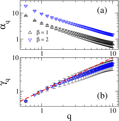
The multifractal dimensions, especially and and their dependence on the parameter in the case of the PBRM model, have been at the focus of several of our works.MTC06 ; MV06 In those works it has been demonstrated that simple phenomenological relations can be identified: and where are fitting constants. These continuous functions are trivial interpolations between the limiting cases of low– and large–, taking the half of the harmonic mean of the two cases. In Ref. [EPL12, ] we generalized and propose the following heuristic expression for an extended range of the parameter
| (10) |
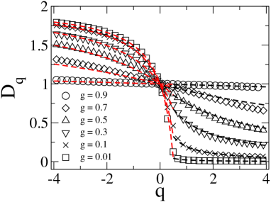
as a global fit for the multifractal dimensions of the PBRM model for both symmetry classes, and . In Fig. 1 we show fits of Eq. (10) to numerically obtained ’s as a function of for some values of for the PBRM model with (the case has been already reported in Ref. [EPL12, ]) and in Fig. 2(a) we plot the values of extracted from the fittings; here, for comparison purposes, we report both cases: and . We observe that Eq. (10) fits reasonably well the numerical for . It is important to stress that Eq. (10) reproduces well the -dependencies predicted analyticallyEM08 for the limits and .

The multifractal dimensions of Fig. 1 were extracted from the linear fit of the logarithm of the inverse mean eigenfunction participation numbers versus the logarithm of , see Eq. (1). was extracted from the linear fit of the mean eigenfunction entropy versus the logarithm of , see Eq. (2). We used system sizes of with . The average was performed over eigenvectors with eigenvalues around the band center of realizations of the random matrices.
We have also verified that
| (11) |
reproduces qualitatively well the -dependencies predicted analyticallyEM08 ; KYC in the small– and large– limits:
| (12) |
Moreover, the parameter must be equal to for Eqs. (10) and (11) to fulfill relation (7).
As a consequence of equating in Eqs. (10) and (11) we get a direct relation
| (13) |
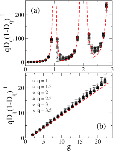
with . We observed that in the range , as plotted in Fig. 2(b), so in this range of values we can write simplified relations between and :
| (14) |
The expression for in Eq. (14) reproduces Eq. (8) exactly for and and approximately for . Moreover, Eq. (14) combined with Eq. (7) allows us to express any in terms of, for example, :
| (15) |
We also noticed that by equating for different ’s from Eq. (14) we could get recursive relations among them:
| (16) |
which in case of taking leads to
| (17) |
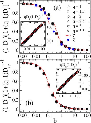
Notice that all these relations can be expressed using the fact that the ratio is independent of . These expressions also provide a relation between the correlation dimension and the information dimension or between the correlation dimension and the compressibility of the spectrum:
| (18) |
It is relevant to add that in the weak multifractal regime, i.e. when , Eq. (18) reproduces the relation given in Eq. (6) with , reported in [CKL96, ].
II.1 The case
For , Eq. (10) cannot be directly applied. However, the regime could also be explored within our approach by the combination of Eq. (10) and the symmetry relationMFME06
| (19) |
implying that it is possible to link the multifractal dimensions with indexes to those with . Therefore, we get
| (20) |
for ; that is, once we know the coefficients for we can use them to get for . Moreover, by the use of Eq. (17) it is possible to write , for , as a function of any specific with . For example,
| (21) |
provides for in terms of the information dimension. Moreover, we can write down relations between and with :
| (22) |
II.2 Wigner delay times
As mentioned in the Introduction, the modeling and analysis of multifractal states in disordered systems at the Anderson–transition has been a subject of intensive research activity for many decades.MJ98 ; EM08 Moreover, since the properties of the closed system, i.e. the fractality of the eigenstates, strongly influence the scattering and transport properties of the corresponding open system, the interest has also been extended to critical scattering systems. In particular, much attention has been focused on the probability distribution functions of the resonance widths and Wigner delay times, MV06 ; MK05 ; OF05 ; MFME06 ; OKG03 ; F03 ; TC99 ; KW02 ; KW02b ; WMK06 as well as the transmission or dimensionless conductance. S90 ; M94 ; M99 ; SO97 ; SOK00 ; SMO00 ; WLS98 ; RS01 ; RMS001 ; TM02 ; SM05 ; JMZ99 ; SZ02 ; MG09a ; MG09b ; MGV10 ; MMV10
Among many relevant results, here we want to focus on those related to Wigner delay times and recall that
- (i)
-
(ii)
for the PBRM model at criticality the typical values of the Wigner delay times scale asMV06
(25) with .
Note that Eqs. (24) and (25) provide a way to probe the properties of a critical system (i.e. the fractality of its eigenstates) by means of scattering experiments. Moreover, we can also relate spectral properties to scattering properties by
- (i)
- (ii)
Also, we can express any as a function of, say, :
| (28) |
Finally, note that we can obtain recursive relations for ’s in analogy to Eq. (16):
| (29) |
or
| (30) |
which leads to
| (31) |
when .
III Numerical results for the PBRM model
In this section we present numerical justification of our analytical relations derived above using the PBRM model.
III.1 Multifractal exponents
In Fig. 3 we plot as a function of for several values of for the PBRM model at criticality with and and observe good correspondence with the analytical prediction for ; that is, we verify the validity of Eq. (14). For completeness in Fig. 3(a) we also include independent numerically obtained values of (taken from Ref. [KS, ]). In the insets of Fig. 3 we plot as a function of , see Eq. (16), which for the PBRM model acquires the simple form
| (32) |
The fact that all curves vs fall one on top of the other makes evident its independence of .
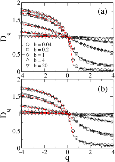
In Fig. 4 we present as a function of for the PBRM model with and for some values of . As black and red dashed lines we also include Eqs. (15), for , and (21), for , respectively. In both equations we used values of we have obtained numerically. We observe very good correspondence between the numerical data and Eqs. (21) and (15) mainly for and , respectively.
III.2 Wigner delay times
We obtain Wigner delay times by turning the isolated system, represented by the PBRM model, into a scattering one by attaching one semi-infinite single-channel lead using perfect coupling. Since we are dealing here with the periodic version of the PBRM model, all sites are bulk sites and the place at which we attach the lead is irrelevant. To compute we use the effective Hamiltonian approach described in Refs. [MK05, ; MV06, ]. For statistical processing a large number of disorder realizations is used. Each disorder realization gives one value of . We used , 100, 200, 400, and 800 getting , , , , and values of , respectively. Then, the exponents [] were extracted from the linear fit of the logarithm of the averaged inverse moments of Wigner delay times [typical Wigner delay times] vs. the logarithm of , see Eq. (24) [Eq. (25)]. We concentrate here on the PBRM model with only.
We start by noticing that if we combine Eqs. (10) and (24) we get a heuristic expression for as a function of :
| (33) |
In Fig. 5 we compare Eq. (33) to the numerically obtained as a function of for some values of . We observe that Eq. (33) fits reasonably well the numerical for . In Fig. 5 we also include independent numerically obtained values of that further verifies the validity of relation (24) [MFME06, ; MK05, ; OF05, ].
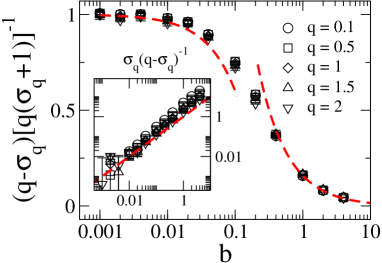
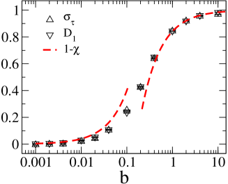
In Fig. 6 we plot as a function of for the PBRM model at criticality; that is, we verify the validity of Eq. (26). We also plot the analytical prediction for given in Eq. (12) and observe good correspondence with the numerical data. In the inset we plot as a function of , see Eq. (29), which for the PBRM model acquires the simple form
| (34) |
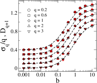
Finally, in Fig. 7 we show as a function of for the PBRM model at criticality with . To test the validity of Eq. (27) we compare with the numerically obtained and with the theoretical prediction for . We again observe good correspondence.
IV Other critical ensembles
Remember that relations (14-18) were obtained form the combination of Eqs. (10) and (11). That is, relations (14-18) are expected to work in particular for the PBRM model at criticality. However, Eqs. (14) reproduce Eqs. (7) and (8), which were shown to be valid for the PBRM model but also for other critical ensembles.BG11 Therefore the question arises to which extent relations (14-18) are valid for critical ensembles different to the PBRM model. So, in the following we verify the validity of Eqs. (14-18) for other well known critical ensembles.
IV.1 Calogero-Moser ensembles
The Calogero–Moser (CM) -particle systems yield three ensembles of Hermitian matrices of the formBG11b ; BG11c
| (35) |
where are independent Gaussian random variables with zero mean and unit variance, is a free parameter which drives the multifractality of the eigenstates, and is one of the three following functions
These ensembles were denoted asBG11b ; BG11c CMR, CMH, and CMT, respectively.
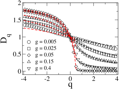
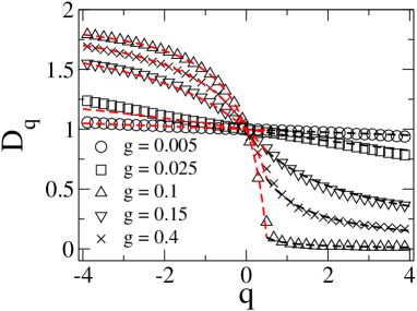
In Figs. 8 and 9 we plot as a function of for the CMR and CMT ensembles, respectively, for several values of . To have an independent verification of our predictions, the data reported in these figures was taken from Ref. [BG11c, ]. We compare the numerical data with our equations for with , Eq. (21), and , Eq. (15); using as input, values of obtained by the interpolation of the curves vs. . We observe for both ensembles that our predictions reproduce reasonably well the numerical data.
IV.2 The Ruijsenaars-Schneider Ensemble and Intermediate quantum maps
The Ruijsenaars-Schneider Ensemble (RSE) proposed in [BGS09, ] is defined as matrices of the form
| (36) |
where , are independent random phases distributed between 0 and , and is a free parameter independent on .
Now, in Fig. 10 we present as a function of for the RSE for several values of . The data was also taken from Ref. [BG11c, ]. As for the CM ensembles, here we observe that our predictions reproduce reasonably well the numerical data for both with and . The values of we used as input in Eqs. (21) and (15) were obtained by the interpolation of the curves vs. .
In fact, in Ref. [EPL12, ] we have already successfully tested the predictions given by Eq. (18) on the RSE. There, we even formulated heuristic expressions for :
| (37) |
and
| (38) |
for and with , respectively. We got the expressions above by substituting and [or and ], obtained analytically in Ref. [BG11, ], into Eq. (14) [or Eq. (15)].
Also, in Ref. [EPL12, ] we tested some of our predictions for a variant of the RSE, introduced in [MGG08, ], with the name of intermediate quantum maps (IQM) model; see also [MGGG10, ]. In this model the parameter of the RSE is replaced by with mod , being the parameter of the IQM model. For the IQM model we substituted or , analytical expressions reported in [MGG08, ], into Eq. (14) or (15), respectively, to get
| (39) |
Here we just want to add that by the use of Eqs. (37) and (38), for the RSE, and Eq. (39), for the IQM model, we can demonstrate the independence of on (already shown for the PBRM model in Fig. 3). In fact, by substituting the above-mentioned expressions into Eq. (16) we get
| (40) |
and
| (41) |
for and with , respectively, for the RSE; and
| (42) |
for the IQM model. Then, In Fig. 11 we plot for the RSE and the IQM model for several values of . We also include the equations given above in red dashed lines. We observe a rather good correspondence between numerical data and Eqs. (40-42).
IV.3 Higher dimensional models
The generalization of Eqs. (14-18) to higher dimensional systems () can be done if is replaced by in Eqs. (14-18). Then, below we explore the applicability of our results to the Quantum Hall transition in and the Anderson transition in .
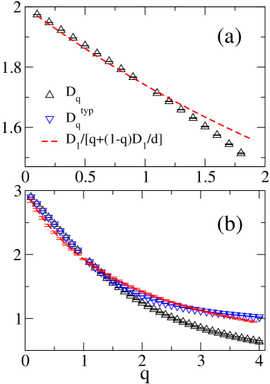
In Fig. 12(a) we plot as a function of for the Quantum Hall transition (QHT). The data for was taken from [EMM08, ]. We also include the prediction for given by Eq. (15) (where has been replaced by ) using [EMM08, ]. We observe that the prediction of Eq. (15) is a reasonably good approximation for in the interval .
In Fig. 12(b) we plot and as a function of , for the 3d Anderson model at criticality, together with the prediction for given by Eq. (15) (where has been replaced by ) using [RVSR10, ]. The data for and was taken from [thesis, ]. The multifractal dimensions were extracted from the scaling of the typical participation numbers with the system size , from the relation
| (43) |
We observe that the prediction of Eq. (15) is reasonably good for with . In contrast, Eq. (15) do not reproduce the numerical when . We have also substituted (obtained from the interpolation of the data from [thesis, ]) into Eq. (15) but the resulting curve is very similar to that with , so we do not show it in Fig. 12(b).
V Applicability to deterministic models
In the previous section we have verified that relations (14-18) are valid for critical random matrix ensembles in 1d and also, to some extent, to higher dimensional models at criticality. The common feature in the systems used above is the presence of multifractal eigenstates. However, note that not only disordered models produce them. It is well known that deterministic models having self-similar potentials also possess multifractal eigenstates, see for example [FKT89, ; WS12, ]. Moreover, multifractal objects can be expressly constructed by the use of iteration algorithms. As examples we can mention the Cantor set and the set produced by baker’s map.
Below, we test the applicability of our expressions relating multifractal exponents now to the multifractal eigenstates of a tight-binding model having a self-similar potential and to multifractal sets produced by iteration algorithms.
V.1 Off–diagonal one dimensional Fibonacci lattice
According to Fujiwara et al. [FKT89, ] the multifractal spectrum of a one–dimensional Fibonacci sequence can be represented by the inflation rule , where and , so and so on. In this case the Schrödinger equation
has a multifractal solution at the bandcenter, . Then, by defining the parameter the generalized dimensions of the eigenstates take the form FKT89
| (44) |
where is the golden mean, and . Hence, the information dimension and the correlation dimension read as
| (45) |
and
| (46) |
respectively.
Then, in Fig. 13 we plot , computed from Eq. (44), as a function of for the Fibonacci lattice for several values of . The dashed line is the prediction for given by Eq. (15) with calculated from Eq. (45). Again, as for the eigenstates of disordered models, here we observe that Eq. (15) reproduces rather well the multifractal dimensions of the eigenstates of the Fibonacci lattice, mainly in the range of .

V.2 The 2–measure, 1–scale Cantor set or binomial branching process
In order to generate a multifractal distribution we use a Cantor set with two measures.Cantor Take the interval and divide it into two parts, which in our case can cover the whole interval, and even we can choose them to be equal. So let us partition the unit interval into two equal halves. Now let us introduce another measure: let us associate the probability with one of the intervals and with the other one. Then let us do the same procedure with the two subintervals. In this way we start with the unit interval with probability measure 1 in the 0th approximation, then the 1st iteration gives two half intervals with probabilities and . After the 2nd iteration we get four intervals, with length one-fourth each but with measures , , , and . Proceeding further iteratively the distribution will be a multifractal. Such a distribution may be achieved also using a binomial branching process.MH13
Since the distribution can be obtained in a recursive way, the generalized entropies of these distributions can be traced back to the 1st iteration, so we can write down immediately, see [VPJP96, ; MH13, ] for details. Therefore,
| (47) |
and
| (48) |
where the factor comes from the fact that the unit interval has been divided into two pieces of length or in other words the branching is always two-fold.
In Fig. 14 we plot , computed from Eq. (47), as a function of for the Cantor set for several values of . The dashed line is the prediction for given by Eq. (15) with calculated from Eq. (48). Again, as for the Fibonacci lattice, we observe that Eq. (15) reproduces rather well the multifractal dimensions of the the Cantor set, mainly in the range of .


V.3 Generalized baker’s map
The generalized baker’s map is defined as a transformation of the unit square with the following rules:Ott We first divide the unit square into two pieces, and ; . We then compress the two pieces in the horizontal direction by different factors, for the piece in and for the piece in ; where . Then we vertically stretch the lower piece by a factor and the upper piece by a factor , so that both are of unit length. We then take the upper piece and place it back in the unit square with its right vertical edge coincident with the right vertical edge of the unit square. Thus, the generalized baker’s map is a mapping of the unit square into two stripes within the square, one in and another one in . Applying the map a second time, maps the two stripes into four stripes. Application of the map more times, results in more stripes of narrower width, where the widths approach zero as approaches infinity. In fact, the intersection of the attractor with a horizontal line is a Cantor set. In the particular case of we haveOtt
| (49) |
Finally, in Fig. 15 we plot , computed from Eq. (49), as a function of for the generalized baker’s map for several values of . The dashed line is the prediction for given by Eq. (15) with calculated from the interpolation of the data vs. . Note that this multifractal is embedded in 2d, so we make the substitution in Eq. (15). We observe that Eq. (15) reproduces well the multifractal dimensions of the generalized baker’s map mainly when . When, we observe good correspondence in the range , only.
VI Conclusions
In this paper we propose heuristic relations on one hand between the generalized multifractal dimensions, and , for a relatively wide range of the parameter , and on the other hand between these dimensions and the level compressibility . As a result we find a general framework embracing an earlier resultCKL96 and a recent one.BG11 Our proposed relations have been corroborated by numerical simulations on: various random matrix ensembles, a deterministic model having a self-similar potential whose eigenstates have multifractal properties, and multifractal objects expressly constructed by the use of iteration algorithms. Of course the analytical relations and the numerical simulations set limitations on the validity for a certain range of the parameter . Therefore our results are obviously approximate. Hence they call for further theoretical as well as numerical investigations.
Moreover, since our relations between the generalized dimensions and the level compressibility allowed us to state a clear link between the spectral and scattering properties of disordered systems at the metal-insulator transition, it may be interesting to explore the consequences of our results on the quantities characterizing the dynamical properties of critical random matrix ensembles; which have been the focus of very recent investigations.KOY11 ; KYSC12 ; GMGG12
We believe that our results may find applications in several recently studied models characterized by multifractal eigenstates; such as deterministic self-similar potentials,FKT89 ; WS12 quantum spin chains,AB12 Dirac fermions in the presence of random magnetic fields,CHHF12 disordered graphene,graphene and other critical random matrix ensembles.BG11 ; FOR09
Acknowledgements.
The authors are greatly indebted to V. Kravtsov for useful discussions. This work was partially supported by VIEP-BUAP (Grant MEBJ-EXC14-I), PIFCA (Grant BUAP-CA-169), the Alexander von Humboldt Foundation, and the Hungarian Research Fund (OTKA) grant K108676.References
- (1) M. Janssen, Phys. Rep. 295, 1 (1998); Int. J. Mod. Phys. B 8, 943 (1994).
- (2) F. Evers and A. D. Mirlin, Rev. Mod. Phys. 80, 1355 (2008).
- (3) A. Richardella, P. Roushan, S. Mack, B. Zhou, D. A. Huse, D. D. Awschalom, and A. Yazdani, Science 327, 665 (2010); S. Faez, A. Strybulevych, J. H. Page, A. Lagendijk, and B. A. van Tiggelen, Phys. Rev. Lett. 103, 155703 (2009); K. Hashimoto, C. Sohrmann, J. Wiebe, T. Inaoka, F. Meier, Y. Hirayama, R. A. Römer, R. Wiesendanger, and M. Morgenstern, Phys. Rev. Lett. 101, 256802 (2008).
- (4) E. Bogomolny and O. Giraud, Phys. Rev. Lett. 106, 044101 (2011).
- (5) E. Bogomolny and O. Giraud, Phys. Rev. E 84, 036212 (2011).
- (6) E. Bogomolny and O. Giraud, Phys. Rev. E 85, 046208 (2012).
- (7) I. Rushkin, A. Ossipov, and Y. V. Fyodorov, J. Stat. Mech. L03001 (2011).
- (8) J. A. Mendez-Bermudez, A. Alcazar-Lopez, and I. Varga, Europhys. Lett. 98, 37006 (2012).
- (9) E. Cuevas and V. E. Kravtsov, Phys. Rev. B 76, 235119 (2007).
- (10) F. Wegner, Z. Phys. B 36, 209 (1980).
- (11) M. Mehta, Random Matrices (Academic Press, Boston, 1991); T. Guhr, A. Müller-Groeling, H. A. Weidenmüller, Phys. Rep. 299, 189 (1998).
- (12) J. T. Chalker, V. E. Kravtsov, and I. V. Lerner, JETP Lett. 64, 386 (1996); R. Klesse and M. Metzler, Phys. Rev. Lett. 79, 721 (1997).
- (13) A. D. Mirlin, Y. V. Fyodorov, F.-M. Dittes, J. Quezada, and T. H. Seligman, Phys. Rev. E 54, 3221 (1996).
- (14) A. D. Mirlin, Phys. Rep. 326, 259 (2000).
- (15) V. E. Kravtsov and K. A. Muttalib, Phys. Rev. Lett. 79, 1913 (1997); V. E. Kravtsov and A. M. Tsvelik, Phys. Rev. B 62, 9888 (2000).
- (16) E. Cuevas, M. Ortuno, V. Gasparian, and A. Perez-Garrido, Phys. Rev. Lett. 88, 016401 (2001).
- (17) I. Varga and D. Braun, Phys. Rev. B 61, R11859 (2000); I. Varga, ibid. 66, 094201 (2002).
- (18) J. A. Méndez-Bermúdez, T. Kottos, and D. Cohen, Phys. Rev. E 73, 036204 (2006).
- (19) J. A. Méndez-Bermúdez and I. Varga, Phys. Rev. B 74, 125114 (2006).
- (20) V. E. Kravtsov, O. M. Yevtushenko, and E. Cuevas, J. Phys. A: Math. Gen. 39, 2021 (2006); J. Phys. A: Math. Theor. 44, 189501 (2011).
- (21) A. D. Mirlin, Y. V. Fyodorov, A. Mildenberger, and F. Evers, Phys. Rev. Lett. 97, 046803 (2006).
- (22) C. Monthus and T. Garel, J. Stat. Mech. P09015 (2010).
- (23) V. E. Kravtsov, private communication.
- (24) J. A. Méndez-Bermúdez and T. Kottos, Phys. Rev. B 72, 064108 (2005).
- (25) A. Ossipov and Y. V. Fyodorov, Phys. Rev. B 71, 125133 (2005).
- (26) A. Ossipov, T. Kottos, and T. Geisel, Europhys. Lett. 62, 719 (2003).
- (27) Y. V. Fyodorov, JETP Letters 78, 250 (2003).
- (28) C. Texier and A. Comtet, Phys. Rev. Lett. 82, 4220 (1999); A. Ossipov, T. Kottos, and T. Geisel, Phys. Rev. B 61, R11411 (2000).
- (29) T. Kottos and M. Weiss, Phys. Rev. Lett. 89 056401, (2002).
- (30) F. Steinbach, A. Ossipov, T. Kottos, and T. Geisel, Phys. Rev. Lett. 85, 4426, (2000).
- (31) M. Weiss, J. A. Méndez-Bermúdez, and T. Kottos, Phys. Rev. B 73, 045103, (2006).
- (32) B. Shapiro, Phys. Rev. Lett. 65, 1510 (1990).
- (33) P. Markoš, Europhys. Lett. 26, 431 (1994).
- (34) P. Markoš, Phys. Rev. Lett. 83, 588 (1999).
- (35) K. Slevin and T. Ohtsuki, Phys. Rev. Lett. 78, 4083 (1997).
- (36) K. Slevin, T. Ohtsuki, and T. Kawarabayashi, Phys. Rev. Lett. 84, 3915 (2000).
- (37) K. Slevin, P. Markoš, and T. Ohtsuki, Phys. Rev. Lett. 86, 3594 (2001).
- (38) X. Wang, Q. Li, and C. M. K. Soukoulis, Phys. Rev. B 58, 3576 (1998).
- (39) M. Rühländer and C. M. Soukoulis, Physica B 296, 32 (2001).
- (40) M. Rühländer, P. Markoš, and C. M. Soukoulis, Phys. Rev. B 64, 172202, 212202 (2001).
- (41) I. Travěnec and P. Markoš, Phys. Rev. B 65, 113109 (2002).
- (42) L. Schweitzer and P. Markoš, Phys. Rev. Lett. 95, 256805 (2005); J. Phys. A: Math. Gen. 39, 3221 (2006).
- (43) M. Jansen, M. Metzler, and M. R. Zirnbauer, Phys. Rev. B 59, 15836 (1999).
- (44) K. Senouci and N. Zekri, Phys. Rev. B 66, 212201 (2002).
- (45) C. Monthus and T. Garel, Phys. Rev. B 79, 205120 (2009).
- (46) C. Monthus and T. Garel, J. Stat. Mech. P07033 (2009).
- (47) J. A. Méndez-Bermúdez, V. A. Gopar, and I. Varga, Phys. Rev. B 82, 125106 (2010).
- (48) A. J. Martínez-Mendoza, J. A. Méndez-Bermúdez, and I. Varga, AIP. Conf. Proc. 1319, 41 (2010).
- (49) K. Slevin, private communication.
- (50) E. Bogomolny, O. Giraud, and C. Schmit, Phys. Rev. Lett. 103, 054103 (2009).
- (51) J. Martin, O. Giraud, and B. Georgeot, Phys. Rev. E 77, 035201(R) (2008).
- (52) J. Martin, I. Garcia-Mata, O. Giraud, and B. Georgeot, Phys. Rev. E 82, 046206 (2010).
- (53) F. Evers, A. Mildenberger, and A. D. Mirlin, Phys. Rev. Lett. 101, 116803 (2008).
- (54) A. Rodriguez, L. J. Vasquez, K. Slevin, and R. A. Römer, Phys. Rev. Lett. 105, 046403 (2010).
- (55) L. J. Vasquez, High precision multifractal analysis in the 3D Anderson model of localization, PhD Thesis, The University of Warwick, 2010.
- (56) T. Fujiwara, M. Kohmoto, and T. Tokihiro, Phys. Rev. B 40, 7413 (1989).
- (57) M. Woloszyn and B. J. Spisak, Eur. Phys. J. B 85, 10 (2012).
- (58) B. Mandelbrot, Fractals: Form, Chance and Dimension (W. H. Freedman, San Francisco, 1977); T. C. Halsey, M. H. Jensen, L. P. Kadanoff, I. Procaccia, and B. Shrainman, Phys. Rev. A 33, 1141 (1986).
- (59) H. Miki and H. Honjo, J. Phys. Soc. of Japan 82, 034002 (2013).
- (60) I. Varga, J. Pipek, M. Janssen, and K. Pracz, Europhys. Lett. 36, 437 (1996).
- (61) E. Ott, Chaos in Dynamical Systems (Cambridge University Press, Cambridge, 2002).
- (62) V. E. Kravtsov, A. Ossipov, and O. M. Yevtushenko, J. Phys. A: Math. Theor. 44, 305003 (2011).
- (63) V. E. Kravtsov, O. M. Yevtushenko, P. Snajberk, and E. Cuevas, Phys. Rev. E 86, 021136 (2012).
- (64) I. Garcia-Mata, J. Martin, O. Giraud, and B. Georgeot, Phys. Rev. E 86, 056215 (2012).
- (65) Y. Y. Atas and E. Bogomolny, Phys. Rev. E 86, 021104 (2012); Phil. Trans. R. Soc. A 372, 20120520 (2014).
- (66) C. C. Chamon, C. Murdy, and X. Wen, Phys. Rev. Lett. 77, 4194 (1996); X. Chen, B. Hsu, T. L. Hughes, and E. Fradkin, Phys. Rev. B 86, 134201 (2012).
- (67) I. Kleftogiannis and S. N. Evangelou, arXiv:1304.5968; J. E. Barrios-Vargas and G. G. Naumis, 2D Mater. 1, 011009 (2014).
- (68) Y. V. Fyodorov, A. Ossipov, and A. Rodriguez, J. Stat. Mech. L12001 (2009).