Replicator dynamics with turnover of players

Abstract

We study adaptive dynamics in games where players abandon the population at a given rate, and are replaced by naive players characterized by a prior distribution over the admitted strategies. We demonstrate how such process leads macroscopically to a variant of the replicator equation, with an additional term accounting for player turnover. We study how Nash equilibria and the dynamics of the system are modified by this additional term, for prototypical examples such as the rock-scissor-paper game and different classes of two-action games played between two distinct populations. We conclude by showing how player turnover can account for non-trivial departures from Nash equilibria observed in data from lowest unique bid auctions.

I Introduction

Perhaps the most important skill for competing agents is the ability to adapt to a changing environment by constantly assessing and modifying their behavior. Consequently, while game theory has been initially mostly focused on the study of equilibria Von Neumann and Morgenstern (1944); Nash (1950), the study of adaptive dynamics has acquired more and more relevance in recent years. Various models have been put forward to capture the learning processes of competing individuals and the resulting evolution of the population Bush and Mosteller (1951); Watkins and Dayan (1992); Kianercy and Galstyan (2012). A key result is that many agent-based algorithms of adaptive dynamics allow for a simple macroscopic description in terms of replicator equations Fisher (1930); Hofbauer (1985); Nowak (2006); Traulsen et al. (2005). In the replicator dynamics, a large population of individuals participate in a game. Let us call $x_{i}$ the fraction of population playing a given strategy, where admissible strategies are labeled as $i=\{1,2,3,\ldots\}$. The time evolution of such fractions is given by:

$$\frac{d}{dt}x_{i}=x_{i}(\pi_{i}(\mathbf{x})-\bar{\pi}(\mathbf{x})),$$ (1)

where $\pi_{i}(\mathbf{x})$ is the frequency-dependent payoff of strategy $i$, and $\bar{\pi}=\sum_{i}x_{i}\pi_{i}$ is the average payoff. In this setting, the initial condition $\mathbf{x}_{i}^{0}$ represent a prior distribution of strategy preferences, before the adaptation process takes place. Approaches based on Eq. (1) have proven successful in describing systems within biology as well as economics Nowak (2006); Maynard Smith (1982); Silverberg (1997). It can be easily shown that stable equilibria of replicator dynamics correspond to Nash equilibria, where no individual can benefit from changing strategy unilaterally Hofbauer (1985); Nash (1951).

Usually, in adaptive dynamics, one has in mind a fixed population of players that acquire experience over time, or biological populations, where offsprings inherit strategies from their parents. However, one can think of a number of concrete examples where games are played in a more open setting, with the possibility of players to leave the game and be replaced by less experienced ones. On the market, new companies are founded while old companies collapse. Within companies, experienced employees retire so that young graduates may start their career. On general grounds, one should expect turnover to have a profound impact on the dynamics of the game and lead to a rich phenomenlogy. In a standard adaptive dynamics all individuals within the population have the same degree of experience. Conversely, here each agent sees a non-trivial mixture of players with different experience levels. While the Nash equilibrium strategy will be optimal against very experienced players, it would not necessarily be the most effective to exploit naive newcomers. Therefore, one can expect adaptive dynamics in this case to converge to equilibria being different from Nash equilibria, and being crucially affected by the rate of turnover, which in turns determines the steady-state structure of the population both in terms of experience and strategies. In such framework, interesting information can be obtained by dissecting the experience composition of each strategy, for example to assess which experience classes are performing better in the game in terms of payoff.

In this paper, we demonstrate how taking into account turnover of players leads macroscopically to a novel variant of the replicator dynamics. We present a derivation of the replicator equation with turnover (Eq. 6) in Section II. In the remainder of the paper, we apply this equation to analyze the effect of turnover in simple evolutionary games. We begin with the simple paradigmatic cases of the rock-paper-scissors game and the set of two-action games played between two different populations. In the latter case, we show how increasing the turnover rate can lead to abrupt change in the equilibrium state caused by bifurcations in the corresponding dynamical system. We conclude the paper by showing how this approach can provide an interpretation for the observed bid distribution in online lowest unique bid auctions.

II Model

We aim at generalizing the replicator equations (1) to situations in which agents are replaced by inexperienced individuals at a rate $p$. Let a large population of players engage in a game with strategies labeled $i=\{1,2,3,\ldots\}$. We divide the players in experiences classes: let $n_{i}(\tau,t)$ be, at time $t$, the number of players having been in the game for a time $\tau$ and playing strategy $i$. The normalization condition for the $n$’s reads:

$$\sum_{i}\sum_{\tau=0}^{\infty}\ n_{i}(\tau,t)=N\quad\forall t,$$ (2)

where $N$ is a fixed total population size. We also define the total fraction of players adopting strategy $i$ at time $t$, $x_{i}(t)=\sum_{\tau=0}^{\infty}n_{i}(\tau,t)/N$. As in the standard replicator equation (1), we introduce the average payoff of strategy $i$, $\pi_{i}(\mathbf{x}(t))$, and the average payoff across strategies $\bar{\pi}=\sum_{i}x_{i}\pi_{i}$.

For the sake of simplicity, we consider a simple adaptive dynamics in which individuals learn of alternative strategies and their average payoff at a rate equal to the fraction of the population that plays by this strategy. Further, an individual playing strategy $i$ learning of a strategy $j$ with a higher average payoff, changes to strategy $j$ with a probability proportional to the payoff difference. Combining these assumptions gives an overall rate of change from strategy $i$ to strategy $j$ equal to $n_{i}x_{j}(\pi_{j}-\pi_{i})$, if $\pi_{j}>\pi_{i}$.

Furthermore, agents leave the population at rate $p$ and are replaced by inexperienced agents. The new agents play each strategy $i$ with a probability proportional to a given distribution $x_{i}^{0}$.

We wish to study the time development of the $n_{i}(\tau,t)$. The learning dynamics encoded in the rules above reads:

$$n_{i}(\tau+1,t+1)-n_{i}(\tau,t)=(1-p)\left(\sum_{j:\,\pi_{j}<\pi_{i}}n_{j}(\tau,t)x_{i}(t)(\pi_{i}-\pi_{j})-\sum_{j:\,\pi_{j}>\pi_{i}}n_{i}(\tau,t)x_{j}(t)(\pi_{j}-\pi_{i})\right)-pn_{i}(\tau,t),$$ (3)

where the first sum represents players changing to strategy $i$ from strategies with lower payoffs, and the second sum represents players changing from strategy $i$ to strategies with higher payoffs. Performing a continuous time limit, the left hand side of the above equation becomes $\partial_{t}n_{i}(\tau,t)+\partial_{\tau}n_{i}(\tau,t)$. We can now integrate the continuous time version of Eq. (3) over $\tau$ and divide by the population size $N$, to obtain a closed evolution equation for the strategies $x_{i}(t)$. Let us recall that $n_{i}(0,t)=\sigma Nx_{i}^{0}$, where the proportionality constant $\sigma$ can be determined by imposing that the final equation preserves the normalization condition. We also assume that, due to the effect of turnover, one has $\lim_{\tau\rightarrow\infty}n_{i}(\tau,t)=0\quad\forall i,t$. After combining the two sums, this results in

$$\frac{d}{dt}x_{i}(t)=(1-p)\sum_{j}x_{j}(t)x_{i}(t)(\pi_{i}-\pi_{j})+\sigma x_{i}^{0}-px_{i}.$$ (4)

Imposing the normalization results in $\sigma=p$. This also implies that the density of players having a given experience level at steady state is exponentially distributed, $\sum_{i}n_{i}(\tau,\infty)=Np\exp(-p\tau)$. If we furthermore use the normalization condition $\sum_{j}x_{j}=1$ and the definition of the average payoff $\bar{\pi}$, we get

$$\frac{d}{dt}x_{i}=(1-p)x_{i}(\pi_{i}-\bar{\pi})+p(x_{i}^{0}-x_{i}).$$ (5)

Upon rescaling time by $1-p$ and define a rescaled turnover rate $\chi=p/(1-p)$, we finally obtain

$$\frac{d}{dt}x_{i}=x_{i}(\pi_{i}-\bar{\pi})+\chi(x_{i}^{0}-x_{i}).$$ (6)

Eq. (6) constitutes the starting point of our analysis. It should be clear that our specific choice of adaptive dynamics is not crucial for deriving Eq. (6), and that the same macroscopic limit could be obtained for other microscopic adaptation rules leading to the replicator equation (1) in the absence of turnover. Eq. (6) can be of course also derived (or justified) heuristically, for example by making an analogy with a (damped) driven dynamical system, where the prior distribution $x^{0}_{i}$ in the right hand side acts as a forcing term. Note that Eq. (6) can be formally recast in replicator form:

$$\frac{d}{dt}x_{i}=x_{i}(\pi_{i}-\bar{\pi})+\chi(x^{0}_{i}-x_{i})\equiv x_{i}(\tilde{\pi}_{i}-\bar{\pi}),$$ (7)

where the “effective payoff” of strategy $i$, $\tilde{\pi}_{i}$, is defined as

$$\tilde{\pi}_{i}=\pi_{i}+\chi\left(\frac{x^{0}_{i}}{x_{i}}-1\right).$$ (8)

In Eq. (7) the average payoff $\bar{\pi}$ does not contain a contribution from the second term in Eq. (8) as its average is zero, so that $\sum_{i}x_{i}\pi_{i}=\sum_{i}x_{i}\tilde{\pi}_{i}$. The mapping in Eq. (7) is valid only in the interior of the simplex ${x_{i}>0\ \forall i,\sum_{i}x_{i}=1}$, while at the boundary the effective payoffs diverge. This situation has some resemblance to the case of evolutionary dynamics in the presence of mutations Hofbauer (1985); Tarnita et al. (2009). The main difference is that in our case the “mutants” are not characterized by new, pure strategies or random strategies, but the mixed distribution $x_{i}^{0}$ of the existing strategies.

The fact that the replicator equation with turnover (6) can be rewritten in replicator form (7) implies that the two equations share several mathematical properties. Among these is that the mean effective payoff for the population can not decrease along any trajectory. If the payoff function is continuous and bounded, it therefore serves as a Lyapunov function Strogatz (2001), which guarantees that all game dynamics either evolve to an equilibrium point or a closed orbit. For the replicator equation without turnover, $\chi=0$, all Nash equilibria of a game are equilibrium points of the dynamics Hofbauer and Sigmund (2003). For positive $\chi$, the equilibrium points are generally different from the Nash equilibria, and we call these the turnover equilibria of the game. In the limit $\chi\to\infty$, agents are insensitive to the rewards and the initial strategy $x_{i}^{0}$ is the only equilibrium point.

III Rock-Paper-Scissors

We now apply the concept of agent turnover to the three-strategy game of rock-paper-scissors. In this well-known, biologically relevant game Frean and Abraham (2001); Kerr et al. (2002); Kirkup and Riley (2004); Nahum et al. (2011); Sinervo and Lively (1996), a large population of players can choose between the strategies rock, paper, and scissors. The average fraction of the population employing each strategy is denoted $x_{R}$, $x_{P}$, and $x_{S}$, respectively. The players are paired randomly in each round. Since the strategies dominate each other cyclically, their payoffs are given by

$$\pi_{R} =x_{S}-x_{P}$$ (9)

$$\pi_{P} =x_{R}-x_{S}$$ (10)

$$\pi_{S} =x_{P}-x_{R}.$$ (11)

Rock-paper-scissors is a zero-sum game, so the average payoff in (6) is always zero. The only Nash equilibrium of the game is when all individuals play randomly, giving them all an average payoff of zero Szabó and Fáth (2007).

When we introduce a player turnover, naïve players that enter the game choose to play rock, paper, or scissors with probability $x^{0}_{R}$, $x^{0}_{P}$, and $x^{0}_{S}$, respectively. Gradually, each individual change strategy according to Eq. (3), resulting in the mean behavior given by Eq. (6).

Figure 1: (Color online) Turnover of players in the rock-paper-scissors game with an initial strategy of $80\%$ rock and $10\%$ paper and scissors. A For $\chi=0$, the average strategy oscillates in a fixed distance from the Nash equilibrium. B For infinite turnover, only the initial strategy $\mathbf{x^{0}}$ is employed. C For intermediate turnovers, the average strategy converges to the turnover equilibrium. D The turnover equilibrium for different values of $\chi$. The equilibrium is displaced towards paper, which dominates the initial strategy. E In the turnover equilibrium, inexperienced players quickly turn away from playing rock. Experienced players only play paper. F Inexperienced players have a large negative payoff, which monotonically increases as the players gain experience. However, since the number of experienced players falls off exponentially, most games are won by players of intermediate experience. In this example, we chose a total population size $N=20$.

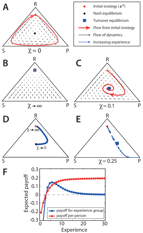
In Fig. 1A-D the time development of the average strategy played is shown for an initial strategy $\mathbf{x}^{0}=(0.8,0.1,0.1)$ biased towards rock and for different values of $\chi$. Similar results are obtained using different initial strategies. In the absence of agent turnover, the strategy of the population oscillates around the Nash equilibrium Szabó and Fáth (2007); Reichenbach et al. (2006). Upon introducing turnover, the initial overrepresentation of players playing rock makes paper a rewarding strategy. As players change strategy towards paper, scissors becomes more rewarding, and so on. In the limit of $\chi\to\infty$, all players remain naïve, so the strategy of the population is equal to the initial strategy.

For intermediate turnover rates, the system undergoes damped or critically damped oscillations towards the turnover equilibrium, where the gradual learning of the players staying in the game exactly balances the exchange of experienced players with naïve players. Thus, agent turnover stabilizes the game dynamics, in a similar way as spatial organization of agents Kerr et al. (2002); Reichenbach et al. (2006); Juul et al. (2012, 2013). The location of the turnover equilibrium depends non-trivially on the strategy of naïve players and on the turnover rate, as shown in Fig. 1D. When $\chi$ is increased from $0$ to $\infty$, the turnover equilibrium shifts from the Nash equilibrium to the strategy distribution of inexperienced players along a curved line. This means that, for a generic value of $\chi$, the turnover equilibrium is not trivially a linear combination of the Nash equilibrium and the naive strategy.

In a traditional game of rock-paper-scissors, the time-averaged payoff of all players is zero in any steady state situation. In the turnover equilibrium, however, the average payoff of players increases monotonically with their experience, such that new, naïve players tend to lose to more experienced players. Fig. 1E shows the average strategy $n_{i}(\tau,\infty)/N$ as a function of the experience level $\tau$, where the turnover is $\chi=0.25$ and the naïve strategy is the same as before . The strategy with the highest payoff is paper, which is the only strategy that very experienced players employ. However, due to the turnover of agents, the number of experienced players falls off exponentially. This causes a radical qualitative difference between the payoff of a given player having an experience level $\tau$ and the total payoff of players in a given experience level. Denoting the turnover equilibrium by $\mathbf{x}^{*}$, the total payoff collected by players with experience $\tau$ is given by $\sum_{i}n_{i}(\tau,\infty)\pi_{i}(\mathbf{x}^{*})$, while the payoff of a single player with this experience is $\sum_{i}n_{i}(\tau,\infty)\pi_{i}(\mathbf{x}^{*})/(\sum_{i}n_{i}(\tau,\infty))...$. The two different payoffs are shown in Fig. 1F as a function of the experience level $\tau$ for a population of 20 players. The figure demonstrates the counterintuitive fact that, while the payoff of each single player increase monotonically with the experience, the majority of the games are won by players with intermediate experience levels.

IV Two-agent two-action games

We now turn to the broad class of games, where two populations can both choose between two strategies. Let us define the mixed strategies as $(x,1-x)$ for the first population and $(y,1-y)$ for the second population. The payoffs obtained by the two populations depend on their joint actions Hofbauer and Sigmund (2003) and are traditionally encoded in payoff matrices $A$ and $B$:

$$\begin{pmatrix}\pi_{1}^{x}\\ \pi_{2}^{x}\end{pmatrix}=\begin{pmatrix}a_{11}&a_{12}\\ a_{21}&a_{22}\end{pmatrix}\begin{pmatrix}y\\ 1-y\end{pmatrix}$$ (12)

$$\begin{pmatrix}\pi_{1}^{y}\\ \pi_{2}^{y}\end{pmatrix}=\begin{pmatrix}b_{11}&b_{12}\\ b_{21}&b_{22}\end{pmatrix}\begin{pmatrix}x\\ 1-x\end{pmatrix},$$ (13)

where $\pi_{1}^{x}$ is the payoff of the first strategy for the first population, and so forth. The two populations are learning concurrently and their turnover rates $\chi_{x}$ and $\chi_{y}$ can in principle be different. The learning dynamics can be obtained from Eq. (6).

$$\frac{d}{dt}x=x(1-x)(\pi_{1}^{x}-\pi_{2}^{x})+\chi_{x}(x^{0}-x)$$ (14)

$$\frac{d}{dt}y=y(1-y)(\pi_{1}^{y}-\pi_{2}^{y})+\chi_{y}(y^{0}-y)$$ (15)

where the equations for the second strategies can be simply obtained from the normalization conditions. In the absence of turnover, this system is known as a bi-matrix replicator equation Hofbauer (1996); Hofbauer and Sigmund (2003). In the turnover equilibrium, which we denote as $(x,y)=(x^{*},y^{*})$, the time derivatives are equal to zero. Upon substituting the expressions (12) and (13) for the payoffs leads to the equations

$$\alpha y^{*}+a_{12}-a_{22}=\chi_{x}\frac{x^{*}-x^{0}}{x^{*}(1-x^{*})},$$ (16)

$$\beta x^{*}+b_{12}-b_{22}=\chi_{y}\frac{y^{*}-y^{0}}{y^{*}(1-y^{*})},$$ (17)

where we have introduced

$$\alpha =a_{11}+a_{22}-a_{21}-a_{12},$$ (18)

$$\beta =b_{11}+b_{22}-b_{21}-b_{12}.$$ (19)

The number of solutions to equations (16) and (17) depends on the sign of the product $\alpha\beta$. When $\alpha\beta<0$, there is always one mixed turnover equilibrium. When $\alpha\beta>0$, the number of turnover equilibria can increase at critical values of the turnover parameter. The derivation of these result can be found in appendix A. In the following, we provide examples for two well-known two-action games belonging to the two categories $\alpha\beta<0$ and $\alpha\beta>0$: the game of matching pennies and a coordination game, respectively.

IV.1 Matching pennies

A simple example of $\alpha\beta<0$ is the zero sum game of matching pennies. Two players secretly turn a penny each to heads or tails and reveal the coins simultaneously. If the pennies match, player one receives a reward $r$ from player two. If they do not, player one pays the reward to player two. This game is characterized by the payoff matrices

$$A=\begin{pmatrix}r&-r\\ -r&r\end{pmatrix}\quad B=\begin{pmatrix}-r&r\\ r&-r\end{pmatrix}.$$ (20)

Figure 2: (Color online) Dynamics of the matching pennies game with $r=2$ and initial strategy $x^{0}=y^{0}=0.3$. Other choices of parameter values yield similar results. A For $\chi=0$, the average strategy oscillates at a fixed distance from the Nash equilibrium. B When a turnover is introduced, the average strategy converges to the turnover equilibrium. Here $\chi_{x}=\chi_{y}=1$. C Expected payoff for population one in the turnover equilibrium for varying turnovers. Above a critical value of $\chi_{y}=2$, the first population will win most games.

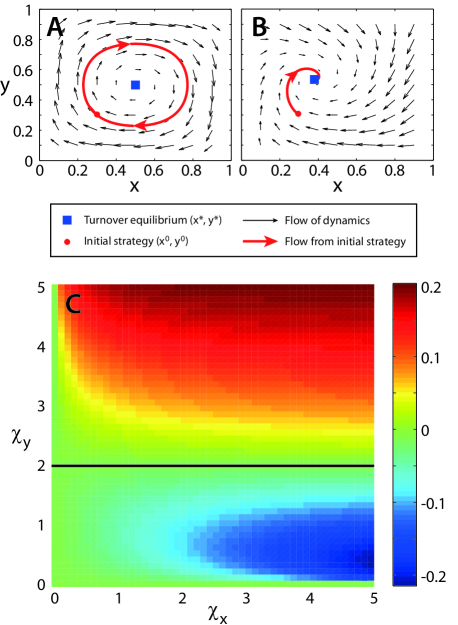
The learning dynamics (14) and (15) with no turnover leads to a marginally stable Nash equilibrium surrounded by concentric closed orbits (see Fig. 2A). When a positive turnover of players is introduced, the Nash equilibrium is perturbed to a stable turnover equilibrium $(x^{*},y^{*})$, as displayed in Fig. 2B. Inserting the payoff matrices into the conditions for turnover equilibrium (16) and (17) gives

$$y^{*}=\frac{1}{2}+\frac{\chi_{x}}{4r}\frac{x^{*}-x^{0}}{x^{*}(1-x^{*})},$$ (21)

$$x^{*}=\frac{1}{2}+\frac{\chi_{y}}{4r}\frac{y^{*}-y^{0}}{y^{*}(1-y^{*})},$$ (22)

Matching pennies is a zero sum game. The expected payoff of population one is positive if the two populations have a tendency of both playing heads or both playing tails, while it is zero if and only if one of the populations chooses their strategy randomly. From Eq. (21) and (22) we see that this happens in the turnover equilibrium if $(x^{*},y^{*})=(1/2,y^{0})$ or $(x^{*},y^{*})=(x^{0},1/2)$. For a given set of initial strategies of the populations, this corresponds to the critical turnover rates

$$\chi_{x,c}=-r\frac{1-2y^{0}}{1-2x^{0}}$$ (23)

$$\chi_{y,c}=r\frac{1-2x^{0}}{1-2y^{0}}.$$ (24)

Equation (23) can only be satisfied if population two wins most games when the initial strategies are employed. In this case, the expected payoff of population one is negative if it has a high turnover, since its equilibrium strategy is close to its initial strategy. If the turnover is decreased below the critical value (23), the first population starts winning more games than it loses regardless of the turnover of population two. Even if population two has an even lower turnover, and thus has an initially superior strategy and more time to gain experience, the equilibrium state remains advantageous for population one.

Likewise, equation (24) only gives a positive critical turnover if population one wins most games when the initial strategies are employed. Here, the payoff for population two goes from being positive to negative when its turnover is increased past the critical value given by (24), regardless of the turnover of the first population. In Fig. 2C, the average payoff for population one is shown for varying turnovers of both populations and the initial strategies $x^{0}=y^{0}=0.3$. In this case, if the turnover of population two is larger than $\chi_{y,c}=2$, population one wins most games.

IV.2 Coordination game

When the payoff matrices of the two populations equal each other, $A=B$, one must necessarily have $\alpha\beta\geq 0$. One example of this is a coordination game, where the two players strive to play the same strategy. We consider the payoff matrices

$$A=B=\begin{pmatrix}6&0\\ 3&2\end{pmatrix},$$ (25)

where $\alpha=\beta=5$. Coordination games with different payoff matrices will have similar dynamical properties. Without player turnover, this game has two pure Nash equilibria where the populations employ the same strategy. In addition, there is a mixed Nash equilibrium at $(x^{*},y^{*})=(2/5,2/5)$ with one stable and one unstable manifold. The stable manifold constitutes the boundary between the basins of attraction of the two pure Nash equilibria (see Fig. 3A). For sufficiently small turnovers, there are three turnover equilibria close to these three Nash equilibria. The initial strategies $(x^{0},y^{0})$ determine which equilibrium state the system goes to.

Figure 3: (Color online) Dynamics of a coordination game with initial strategy $(x^{0},y^{0})=(0.9,0.1)$. A Without turnover, the game has one saddle point Nash equilibrium with stable manifolds that separate the basins of attraction of two pure Nash equilibria. B-C When the initial strategy goes from one basin of attraction to another, the resulting equilibrium state changes discontinuously. Here $\chi_{y}=2$ and $\chi_{x}=0.7$ and $0.72$, respectively. D-E At a critical set of turnover rates two turnover equilibria annihilates in a saddle node bifurcation. Here $\chi_{y}=2$ and $\chi_{x}=0.91$ and $0.92$, respectively. F Bifurcation diagram for turnover equilibria. The point $(x,y)=(0.4,0.9)$ is always an equilibrium. We observe a transcritical bifurcation at $\chi_{x}\approx 0.4$ and the saddle node bifurcation from panels D-E at $\chi_{x}\approx 0.9$. G Expected payoff of population one in the turnover equilibrium for varying turnovers. The dramatic change in payoffs between panel B and C can clearly be seen.

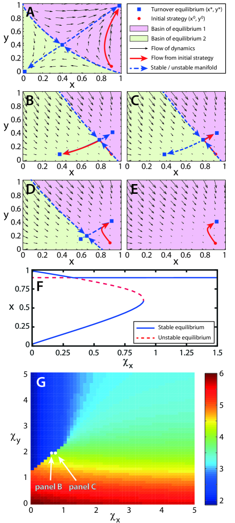
Let us consider a situation of strong initial disagreement $(x^{0},y^{0})=(0.9,0.1)$, where inexperienced players of population one and two tend to employ the first and second strategy, respectively. We fix $\chi_{y}=2$, while varying $\chi_{x}$ as a control parameter. In this case, the point $(x,y)=(0.4,0.9)$ is always an equilibrium of the dynamics. At a critical value, $\chi_{x}\approx 0.71$, the boundary between the basins of attractions passes the initial strategy $(x^{0},y^{0})$ (see Fig. 3B-C), and the steady state changes discontinuously from being dominated by strategy two to strategy one. At the same point, the payoff of both populations increases drastically.

Upon increasing the turnover of the first population even further, the basin of attraction of strategy two suddenly disappears at $\chi_{x}\approx 0.91$. For this value, the saddle node equilibrium annihilates with the turnover equilibrium of strategy two (see Fig. 3D-E). For larger values of $\chi_{x}$, there is only one turnover equilibrium. In this case the number of turnover equilibria changes through a saddle node bifurcation, but for other payoff matrices A, B, a pitchfork bifurcation could occur (see appendix A).

A full bifurcation diagram is shown in Fig. 3F, and the expected payoff of population one is shown in Fig. 3G as a function of the turnover rates. The abrupt change in payoff at a critical set of turnover rates can clearly be seen. The expected payoff of population two follows a similar pattern. In general, a low turnover of either population results in higher payoffs of both populations, since a larger proportion of the players has enough experience to mainly bid on the dominating strategy. However, increasing the turnover may change which equilibrium the system goes to, leading to an increase in the payoff of both players.

V Lowest Unique Bid Auctions

Lowest unique bid auctions have become popular online games, and have recently attracted attention from the scientific community Baek and Bernhardsson (2010); Ostling et al. (2011); Pigolotti et al. (2012). In this game, $N$ players pay an entrance fee to independently bid on an item, e.g. a car. The winner of the auction is the player with the lowest bid not also plaved by another player. The strategies available to each player are the possible integer bids $i=\{1,2,3\ldots\}$.

If a population of players place their bids stochastically according to the distribution $x_{i}$, the average payoff of each strategy is, in the large $N$ limit, proportional to Pigolotti et al. (2012)

$$\pi_{i}=e^{-Nx_{i}}\prod\limits_{j=1}^{i-1}(1-Nx_{i}e^{-Nx_{i}}).$$ (26)

The Nash equilibrium corresponding to the payoffs of Eq. 26 was compared with data from the auctions website auctionair.co.uk in Pigolotti et al. (2012). An excellent agreement between the Nash equilibrium and the data was found for low to intermediate values of $N$. In larger auctions, the bidding distribution departed from the Nash equilibrium and was more resemblant of an exponential distribution

$$x_{i}^{0}=\frac{e^{-\beta i}}{\sum_{i}e^{-\beta i}}.$$ (27)

where the fitted value of the exponential constant was $\beta\approx 0.02$. On general theoretical grounds, one can argue that the exponential bidding strategy is the expected prior distribution for inexperienced players, with limited information about the game, that want to avoid the cost of a large bid Pigolotti et al. (2012); Goeree and Holt (1999).

Using (26) and (27), we test here the hypothesis that the apparent change of behavior from small to large auction sizes is caused by agent turnover. Note that changing the turnover rate $\chi$ in (6) is equivalent to multiplying the payoff function (26) with a constant and rescaling time. As it is also problematic to infer a natural time scale of adaptation from the data, we leave the value of $\chi$ as a fitting parameter.

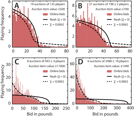
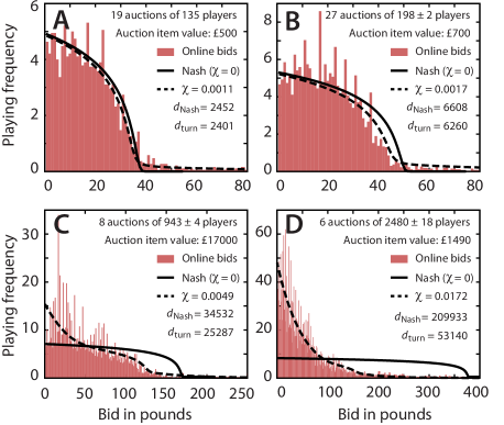
Fig. 4 compares empirical data from 60 online auctions with varying number of players to the respective Nash equilibria and turnover equilibria for a least square fitted value of $\chi=0.0062$. We define the squared distance $d$ between the empirical data and the turnover and Nash equilibria as

$$d_{turn}=N^{2}\sum_{i}(x_{i}^{emp}-x_{i}^{*})^{2}$$ (28)

$$d_{Nash}=N^{2}\sum_{i}(x_{i}^{emp}-x_{i}^{Nash})^{2}$$ (29)

where $\mathbf{x}^{emp}$ is obtained from the frequencies, $\mathbf{x}^{Nash}$ is the theoretical Nash equilibrium, and the sum runs over all bids and all auctions. Using these definitions we get $d_{turn}=89084$ and $d_{Nash}=253526$. In Pigolotti et al. (2012) it is shown that, if the bids were randomly drawn from the theoretical distribution, the squared distance is expected to be equal to the combined number of bidders $d_{exp}=\sum N=30335$. This shows that the turnover equilibria describe the bidding distributions much better than the Nash equilibria, introducing just a single free parameter.

In small auctions, both the Nash equilibrium and the turnover equilibrium fit the data well, but the latter also captures the fat tail of the empirical distribution. In larger auctions, the Nash equilibrium fails to predict the observed distribution of bids, while the turnover equilibrium fits the data remarkably well.

It should be reminded that, while the exponential strategy distribution for large $N$ is plugged into the model empirically as a prior, it is still remarkable that, for the same value of $\chi$, the resulting equilibrium is relatively close to the prior for large $N$ and closer to the Nash equilibrium for smaller values of $N$. The reason stems from the growth of the adaptation time of the replicator dynamics with the auction size $N$ (see Pigolotti et al. (2012)). The consequence if, even at equal turnover rate $\chi$, players have sufficient time to adapt for small auction size but not for larger auctions. Clearly, one could get an even better fit by letting $\chi$ vary as a function of $N$, as one could have different kinds of players and therefore different turnovers for different auction types, as exemplified in Appendix B. We do not present a systematic study of the dependence of $\chi$ on $N$, as it is beyond the scope of this paper. Our main point here is to show that, even in the simple case of a fixed $\chi$, the replicator equation with turnover is useful to model a real-life game and can help conceptualizing non-trivial discrepancies between observed strategy distributions and Nash equilibria. Finally, in Appendix B we show that, in the case of larger auctions, the distance from the Nash equilibrium does not seem to depend on time. This fact further supports the presence of a steady effect, like the turnover mechanism proposed here, preventing the population to reach the Nash equilibrium.

Figure 4: (Color online) Bidding frequencies in online lowest unique bid auctions compared to the theoretical Nash equilibrium and the turnover equilibrium for a constant $\chi=0.0062$. Different panels show auctions with items of different value and different numbers of players. For small auction sizes both the Nash and the turnover equilibrium fit the empirical bidding distributions. In larger auctions the turnover equilibrium fits the data much better than the Nash equilibrium. This is due to a long adaptation time for players in large auctions.

VI Discussion and conclusion

In this paper we have extended the theoretical framework of the replicator equation by considering the effect of agent turnover, a phenomenon that is in principle present in many game theoretical contexts. Our model provides a simple and compact description of the dynamics of the average strategies in the population, and at the same time allows for dissecting the behavior of players having different experience levels. The study of experience-dependent payoffs can bring to counterintuitive results, as we demonstrated in the simple case of a Rock-Paper-Scissor game. When turnover is introduced, the game dynamics become richer. We have shown that it is possible to encounter bifurcations of turnover equilibria, and that the equilibrium strategy can change discontinuously with the turnover rate.

The simplicity and flexibility of the approach proposed in this paper can be of use to analyze several games of practical importance. For example, we have shown here how turnover of agents can help explaining adaptation in online games, where experienced players may exploit the naïve strategies of new players. Our comparison with a dataset of bidding distributions in online lowest unique bid auctions shows that our model is able to describe the empirical steady state distributions far better than the Nash equilibrium. We expect that similar results can be obtained by studying data from other games.

The concepts presented here suggest an interesting analogy with the idea of cognitive hierarchy Costa-Gomes et al. (2001); Camerer et al. (2004); Wright and Leyton-Brown (2010) in human learning, where players are classified according to the number of reasoning steps they are able to make. In this scheme, non-reasoning players are reminiscent of inexperienced players in the present model, and players with more reasoning steps can be compared more to experienced players. In this perspective, the model proposed here provides a framework in which a cognitive hierarchy emerges naturally from the dynamical equilibrium between adaptation and turnover. Indeed, a cognitive hierarchy model has previously been applied to describe the bidding distributions lowest unique bid auctions Ostling et al. (2011). In the authors’ of Ref. Ostling et al. (2011) own words, “the cognitive hierarchy model $\ldots$ should be viewed as a potential stepping stone to an investigation using a formal learning model”. Our work is one proposal of such a learning model.

It is known that a fraction of non-rational, influenceable players may change the game dynamics considerably Halpern and Stern (1998); Nowak et al. (2000); Lorentziadis (2012). In a recent study Couzin et al. (2011), a population of fish were made up of three subgroups: a large group of fish with a small preference for going to one place in the aquarium, a smaller group with a strong preference for another place, and a group of untrained fish with no prior preference. The study showed, both through simulations and experiment, that there exists a critical size of the untrained group above which the entire population goes to the place prefered by group one, and below which the minority of group two dictates where the population goes. This resembles our results for two-agent two-action coordination games, where a critical turnover of agents changes the turnover equilibrium from being dominated by one strategy to the other.

In our model we assume a constant turnover of agents in time, which leaves one free fitting parameter. However, changing the turnover is mathematically equivalent to scaling the expected payoff of all strategies together with a time scaling. Since the absolute value of the payoff is often treated as a free parameter when analyzing experiments of learning dynamics, this does not increase in general the number of fitting parameters in such an analysis. Furthermore, if the absolute values of the payoffs are known, one can in principle measure the turnover rate of agents and avoid having a free fitting parameter.

In conclusion, we have shown how a steady turnover of agents, which is present in most real-life games, can change the qualitative dynamics of a game. The simplicity and generality of the framework presented here makes it a natural candidate to describe adaptation in a population participating in a game and subject to turnover.

Appendix A Number of turnover equilibria in two-agent two-action games

In this appendix, we show that the number of possible turnover equilibria in two-agent two-action games is dependent on the sign of the product $\alpha\beta$, where $\alpha$ and $\beta$ are given by (18) and (19).

The conditions for turnover equilibrium are given by (16) and (17). Expressing $y^{*}$ as a function of $x^{*}$, this can be written as

$$y^{*}(x^{*})=\frac{\chi_{x}}{\alpha}\frac{x^{*}-x^{0}}{x^{*}(1-x^{*})}-\frac{a_{12}-a_{22}}{\alpha},$$ (30)

$$\beta x^{*}+b_{12}-b_{22}=\chi_{y}\frac{y^{*}(x^{*})-y^{0}}{y^{*}(x^{*})(1-y^{*}(x^{*}))}\equiv g(x^{*}),$$ (31)

where we defined the composite function $g(x^{*})$. Notice that $\lim_{x^{*}\rightarrow 0}g(x^{*})=\lim_{x^{*}\rightarrow 1}g(x^{*})=0$ and that $g(x^{*})$ has two singularities for values of $x^{*}$ such that $y^{*}=0$ and $y^{*}=1$. Since $0\leq y^{*}\leq 1$, we will focus on the interval of $g(x^{*})$ between the two singularities.

Figure 5: (Color online) The number of turnover equilibria in a two-action two-agent game as determined by a graphical solution of equation 31. A When $\alpha\beta<0$ the two functions have opposite slopes and hence intersect exactly once in the relevant interval $0<y^{*}<1$. Here the matching pennies game is illustrated with the parameters of Fig. 2B. B-C When $\alpha\beta>0$ the slope of the functions have the same sign, and new turnover equilibria can appear through bifurcations. Here the bifurcation in the coordination game of Fig. 5B-C is shown, except that $\chi_{x}$ is changed from to $0.8$ to $1$ between panels B-C.

Let us investigate the derivative $\partial g/\partial x^{*}$. From Eq. (30) and (31) we get

$$\frac{\partial y^{*}}{\partial x^{*}} =\frac{\chi_{x}}{\alpha}\frac{(x^{*}-x^{0})^{2}+x^{0}-{x^{0}}^{2}}{(1-x^{*})^{2}{x^{*}}^{2}}$$ (32)

$$\frac{\partial g}{\partial x^{*}} =\chi_{y}\frac{(y^{*}-y^{0})^{2}+y^{0}-{y^{0}}^{2}}{(1-y^{*})^{2}{y^{*}}^{2}}\frac{\partial y^{*}}{\partial x^{*}}.$$ (33)

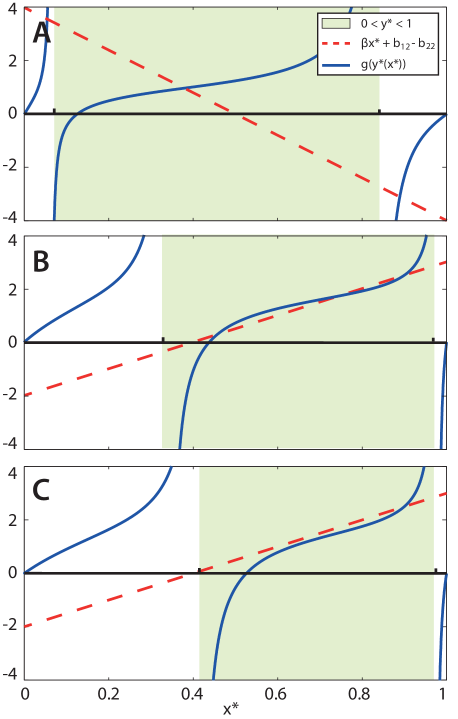
Since $x^{0}$ and $y^{0}$ are probabilities, we always have $x^{0}>{x^{0}}^{2}$ and $y^{0}>{y^{0}}^{2}$. The fractions in Eq. (32) and (33) are therefore positive, so the derivative $\partial g/\partial x^{*}$ must have the same sign as $\alpha$. This means that $g(x^{*})$ is either increasing or decreasing monotonically, depending on the sign of $\alpha$.

If $\alpha\beta<0$, the line $\beta x^{*}+b_{12}-b_{22}$ and the function $g(x^{*})$ have opposite slopes, and therefore intersect exactly once. It follows from (31) that there is always exactly one turnover equilibrium. In Fig. 5A, this is illustrated for the matching pennies game with the same parameters as Fig. 2B.

If $\alpha\beta>0$, the line $\beta x^{*}+b_{12}-b_{22}$ and the function $g(x^{*})$ are either both increasing or both decreasing. Therefore, they can in principle intersect any odd number of times. Hence, it is possible to have multiple turnover equilibria, and these can appear or annihilate in pairs through either saddle point bifurcations or pitchfork bifurcations. Fig. 5B-C shows a saddle node bifurcation in the coordination game with the same parameters as Fig. 3D-E, except we have set $\chi_{x}$ equal to $0.8$ and $1$, respectively, to show a clearer bifurcation.

Appendix B Additional analysis of the lowest unique bid auction data

In this Appendix, we present additional results on the lowest unique bid auction dataset used in Section V. Fig. 6 shows how letting $\chi$ as an independent fitting parameter for each auction size leads to very good fits of the bidding distributions in all cases. The fitted values suggest a higher turnover rate for larger auction sizes, which is reasonable considering for example that larger auctions typically involve larger bidding fees. Furthermore, we see from the combined distances (28) and (29) presented in Fig. 6 that we always have $d_{turn}<d_{Nash}$, so the turnover equilibria always fit the empirical data better than the Nash equilibria, but that this is most significant for large auction sizes. Both equilibria describe the bidding distributions well in small auctions. Notice however that the prior distribution $x_{0}$ has been obtained from the larger auction sizes, so that estimates of $\chi$ in the large auction cases can be affected by overfitting.

Figure 6: (Color online) Same data as Fig. 4, but this time the turnover parameter $\chi$ is fitted independently in each plot. The fitted value of $\chi$ and the total distances between the empirical bidding distributions and the turnover and Nash equilibria, respectively, are indicated in each legend.

Finally, in Fig. 7 we show the evolution of the distance (29) to the Nash equilibrium in series of auctions having similar number of players $N=1398\pm 74$. The exact date of each auction was not available, so that data are plotted simply as a function of the time ordering of the auctions.

Figure 7: (Color online) Distance from the Nash equilibrium for 14 auctions having $N=1398\pm 74$, as a function of the time order of the auctions. The straight line is a fitted linear regression, with slope $m=1\pm 140$.

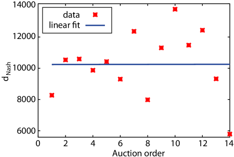
It is easy to demonstrate that, if players bid according to the Nash equilibrium, the expected value of $d$ is $N$ (see Pigolotti et al. (2012)). A value of $d$ significantly larger than $N$ signals a departure from the Nash equilibrium. Fitting the data with a linear regression yields a slope $m=1\pm 140$ that clearly does not allow for refuting the null hypothesis of no temporal trend. This suggests the presence of a mechanism keeping the population at a finite distance from the Nash equilibrium, as the turnover mechanism proposed in this paper.

References

- Von Neumann and Morgenstern (1944) J. Von Neumann and O. Morgenstern, Theory of Games and Economic Behavior (Princeton University Press, 1944).
- Nash (1950) J. Nash, Proc. Natl. Acas. Sci. 36, 48 (1950).
- Bush and Mosteller (1951) R. Bush and F. Mosteller, Psychological Review 58, 313 (1951).
- Watkins and Dayan (1992) C. Watkins and P. Dayan, Machine learning 8, 279 (1992).
- Kianercy and Galstyan (2012) A. Kianercy and A. Galstyan, Physical Review E 85, 041145 (2012).
- Fisher (1930) R. Fisher, The Theory of Natural Selection (Oxford University Press, London, 1930).
- Hofbauer (1985) J. Hofbauer, Journal of mathematical biology 23, 41 (1985).
- Nowak (2006) M. Nowak, Evolutionary Dynamics: Exploring the Equations of Life (Belknap Press, 2006).
- Traulsen et al. (2005) A. Traulsen, J. C. Claussen, and C. Hauert, Phys. Rev. Lett. 95, 238701 (2005).
- Maynard Smith (1982) J. Maynard Smith, Evolution and the theory of games (Cambridge University Press, 1982).
- Silverberg (1997) G. Silverberg, Evolutionary modeling in economics: recent history and immediate prospects (Citeseer, 1997).
- Nash (1951) J. Nash, The Annals of Mathematics 54, pp. 286 (1951).
- Tarnita et al. (2009) C. E. Tarnita, T. Antal, and M. A. Nowak, Journal of theoretical biology 261, 50 (2009).
- Strogatz (2001) S. Strogatz, Nonlinear dynamics and chaos: with applications to physics, biology, chemistry and engineering (Perseus Books Group, 2001).
- Hofbauer and Sigmund (2003) J. Hofbauer and K. Sigmund, Bulletin of the American Mathematical Society 40, 479 (2003).
- Frean and Abraham (2001) M. Frean and E. R. Abraham, Proceedings of the Royal Society of London. Series B: Biological Sciences 268, 1323 (2001).
- Kerr et al. (2002) B. Kerr, M. A. Riley, M. W. Feldman, and B. J. M. Bohannan, Nature 418, 171 (2002).
- Kirkup and Riley (2004) B. Kirkup and M. Riley, Nature 428, 412 (2004).
- Nahum et al. (2011) J. Nahum, B. Harding, and B. Kerr, Proceedings of the National Academy of Sciences 108, 10831 (2011).
- Sinervo and Lively (1996) B. Sinervo and C. Lively, Nature 380, 240 (1996).
- Szabó and Fáth (2007) G. Szabó and G. Fáth, Physics Reports 446, 97 (2007).
- Reichenbach et al. (2006) T. Reichenbach, M. Mobilia, and E. Frey, Phys. Rev. E 74, 051907 (2006).
- Juul et al. (2012) J. Juul, K. Sneppen, and J. Mathiesen, Phys. Rev. E 85, 061924 (2012).
- Juul et al. (2013) J. Juul, K. Sneppen, and J. Mathiesen, Phys. Rev. E 87, 042702 (2013).
- Hofbauer (1996) J. Hofbauer, Journal of mathematical biology 34, 675 (1996).
- Baek and Bernhardsson (2010) S. K. Baek and S. Bernhardsson, Fluctuation and Noise Letters 1, 61 (2010).
- Ostling et al. (2011) R. Ostling, J. Wang, E. Chou, and C. Camerer, American Economic Journal: Microeconomics 3, 1 (2011).
- Pigolotti et al. (2012) S. Pigolotti, S. Bernhardsson, J. Juul, G. Galster, and P. Vivo, Phys. Rev. Lett. 108, 088701 (2012).
- Goeree and Holt (1999) J. K. Goeree and C. A. Holt, Proceedings of the National Academy of Sciences 96, 10564 (1999).
- Costa-Gomes et al. (2001) M. Costa-Gomes, V. Crawford, and B. Broseta, Econometrica 68, 1193 (2001).
- Camerer et al. (2004) C. Camerer, T.-H. Hong, and J.-K. Chong, The Quarterly Journal of Economics pp. 861–898 (2004).
- Wright and Leyton-Brown (2010) J. R. Wright and K. Leyton-Brown, Proceedings of the Twenty-Fourth AAAI Conference on Artificial Intelligence pp. 901–907 (2010).
- Halpern and Stern (1998) J. Halpern and R. Stern, Debating Rationality: Non Rational Aspects of Organizational Decision Making, Frank W. Pierce Memorial Lectureship and Conference Series (Ilr Press/Cornell, 1998).
- Nowak et al. (2000) M. Nowak, K. Page, and K. Sigmund, Science 289, 1773 (2000).
- Lorentziadis (2012) P. L. Lorentziadis, European Journal of Operational Research 217, 653 (2012).
- Couzin et al. (2011) I. Couzin, C. Ioannou, G. Demirel, T. Gross, C. Torney, A. Hartnett, L. Conradt, S. Levin, and N. Leonard, science 334, 1578 (2011).